The Origin of the Large-Scale Structure
in the Universe:

Theoretical and Statistical Aspects
by
YEINZON RODRÍGUEZ GARCÍA
Physicist, MSc
A thesis submmited in partial fulfillment
of the requirements for the degree of
Doctor of Philosophy
in
Physics
LANCASTER UK
LANCASTER UNIVERSITY
FACULTY OF ENVIRONMENTAL AND NATURAL SCIENCES
DEPARTMENT OF PHYSICS
2005

To Luz Yasmid.
                                                                                Three years = one life.

Men in their arrogance claim to understand the nature of creation,
             and devise elaborate theories to describe its behaviour. But always
             they discover in the end that God was quite a bit more clever than
                                                                                                they thought.
                                                    Sister Miriam Godwinson,
                                                    “We Must Dissent”

Begin with a function of arbitrary complexity. Feed it values,
                 “sense data”. Then, take your result, square it, and feed it back
                        into your original function, adding a new set of sense data.
                  Continue to feed your results back into the original function ad
            infinitum. What do you have? The fundamental principle of human
                                                                                              consciousness.
                                                    Academician Prokhor Zakharov,
                                                    “The Feedback Principle”

Einstein would turn over in his grave!
                                       Not only does God play dice… the dice are loaded.
                                                    Chairman Sheng-ji Yang,
                                                    “Looking God in the Eye”

The supreme task of the physicist is to arrive at those
                             universal elementary laws from which the cosmos can be
                                                                           built up by pure deduction.
                                                    Albert Einstein

Beware, you who seek first and final principles, for you are
                    trampling the garden of an angry God and he awaits you just
                                                                              beyond the last theorem.
                                                    Sister Miriam Godwinson,
                                                    “But for the Grace of God”

Abstract

We review some theoretical and statistical aspects of the origin of the large-scale structure in the Universe, in view of the two most widely known and accepted scenarios: the inflaton scenario (primordial curvature perturbation $\zeta$ generated by the quantum fluctuations of the light scalar field $\varphi$ that drives inflation, named the inflaton), and the curvaton scenario ($\zeta$ generated by the quantum fluctuations of a weakly coupled light scalar field $\sigma$ that does not drive inflation, named the curvaton). Among the theoretical aspects, we point out the impossibility of having a low inflationary energy scale in the simplest curvaton model. A couple of modifications to the simplest setup are explored, corresponding to the implementation of a second (thermal) inflationary period whose end makes the curvaton field ‘heavy’, triggering either its oscillations or immediate decay. Low scale inflation is then possible to attain with $H_{\ast}$ (the Hubble parameter a few Hubble times after horizon exit) being as low as $1$ TeV. Among the statistical aspects, we study the bispectrum $B_{\zeta}(k_{1},k_{2},k_{3})$ of $\zeta$ whose normalisation ${f_{\rm NL}}$ gives information about the level of non-gaussianity in the primordial curvature perturbation. In connection with ${f_{\rm NL}}$, several conserved and/or gauge invariant quantities described as the second-order curvature perturbation have been given in the literature. We review each of these quantities showing how to interpret one in terms of the others, and analyze the respective expected ${f_{\rm NL}}$ in both the inflaton and the curvaton scenarios as well as in other less known models for the generation of primordial perturbations and/or non-gaussianities. The $\delta N$ formalism turns out to be a powerful technique to compute ${f_{\rm NL}}$ in multi-component slow-roll inflation, as the knowledge of the evolution of some family of unperturbed universes is the only requirement. We present for the first time this formalism and apply it to selected examples.

Contents

1. 1 Introduction
2. 2 Two mechanisms for the origin of the large-scale structure
   1. 2.1 Introduction
   2. 2.2 Metric perturbations and the primordial curvature perturbation $\zeta$
      1. 2.2.1 First-order perturbations in the FRW line element: classification and number of degrees of freedom
      2. 2.2.2 The curvature perturbation $\psi$ and its non-invariance under infinitesimal coordinate transformations
      3. 2.2.3 The gauge-invariant curvature perturbation $\zeta$
   3. 2.3 Inflation and its effect on the spectrum of perturbations of a non-dominating massless scalar field during a de Sitter stage
      1. 2.3.1 Inflation
      2. 2.3.2 Spectrum of perturbations of a non-dominating massless scalar field during a de Sitter stage
   4. 2.4 The curvaton scenario: an example of a non-dominating light scalar field during a quasi de Sitter stage
      1. 2.4.1 Spectrum of perturbations of a non-dominating light scalar field during a quasi de Sitter stage
      2. 2.4.2 The curvaton scenario
   5. 2.5 The inflaton scenario
      1. 2.5.1 The slow-roll conditions
      2. 2.5.2 Spectrum of perturbations of a dominating light scalar field during a quasi de Sitter stage
      3. 2.5.3 The spectrum of $\zeta$ in the inflaton scenario
   6. 2.6 Gravitational waves
   7. 2.7 Conclusions
3. 3 Low scale inflation and the curvaton mechanism
   1. 3.1 Introduction
   2. 3.2 The bounds on the scale of inflation
      1. 3.2.1 Curvaton physics considerations
      2. 3.2.2 The main bound on the scale of inflation
      3. 3.2.3 Other bounds related to curvaton decay
   3. 3.3 The case of a heavy curvaton
      1. 3.3.1 The thermal inflation model
      2. 3.3.2 Required parameter space
      3. 3.3.3 Solution to the moduli problem
   4. 3.4 Conclusions
4. 4 Low scale inflation and the immediate heavy curvaton decay
   1. 4.1 Introduction
   2. 4.2 Thermal inflation and the immediate heavy curvaton decay
      1. 4.2.1 The flaton-curvaton coupling constant $\lambda$
      2. 4.2.2 The bare curvaton mass $m_{\sigma}$
   3. 4.3 Some useful remarks
   4. 4.4 Conclusions
5. 5 Non-gaussianity from the second-order cosmological perturbation
   1. 5.1 Introduction
   2. 5.2 Two definitions of the curvature perturbation
      1. 5.2.1 Preliminaries
      2. 5.2.2 Two definitions of the curvature perturbation
   3. 5.3 Slow-roll inflation and a third definition
      1. 5.3.1 Single-component inflation
      2. 5.3.2 Multi-component inflation
      3. 5.3.3 A third definition of the curvature perturbation
   4. 5.4 The evolution of the curvature perturbation
      1. 5.4.1 Heavy, light and ultra-light fields
      2. 5.4.2 The evolution of the curvature perturbation
   5. 5.5 Non-gaussianity
      1. 5.5.1 Defining the non-gaussianity
      2. 5.5.2 Observational constraints on the non-gaussianity
   6. 5.6 The initial non-gaussianity
      1. 5.6.1 Single-component inflation
      2. 5.6.2 Multi-component inflation
   7. 5.7 The evolution after horizon exit
      1. 5.7.1 Single-component inflation and $\zeta^{\rm A}_{2}$
      2. 5.7.2 Multi-component inflation
      3. 5.7.3 Preheating
      4. 5.7.4 The curvaton scenario
      5. 5.7.5 The inhomogeneous reheating scenario
   8. 5.8 Conclusions
6. 6 The inflationary prediction for primordial non-gaussianity
   1. 6.1 Introduction
   2. 6.2 Defining the curvature perturbation
   3. 6.3 The inflationary prediction
   4. 6.4 Non-gaussianity
      1. 6.4.1 The bispectrum
      2. 6.4.2 Cosmological perturbation theory
   5. 6.5 The $\delta N$ formalism in some multi-component models
      1. 6.5.1 A two-component inflation model
      2. 6.5.2 The curvaton model
      3. 6.5.3 Another two-component model
   6. 6.6 Conclusions
7. 7 Conclusions
8. A ${f_{\rm NL}}$ from the $\delta N$ formalism

Chapter 1 Introduction

The Friedmann-Robertson-Walker (FRW) cosmological model (known also as the standard or Big-Bang cosmological model) [72, 186, 187, 188, 220] is the successful framework that describes the observed properties of the Universe: homogeneity and isotropy at large scales, Hubble expansion, and almost 14 billion years of evolution in agreement with globular clusters and radioactive isotopes dating. The additional predictions of the cosmic background radiation, confirmed by Penzias and Wilson’s discovery in 1965 [46, 168], and the relative abundances of light elements [6, 7, 73, 87, 165, 219, 221] in full agreement with observation, have established a solid base for the study of the Universe throughout its history, turning the old speculative cosmology into well established and experimentally supported science [75].

The introduction of a period of exponential expansion (called inflationary) [5, 79, 117], prior to the Big-Bang, brought an elegant solution to the horizon, flatness, and unwanted relics problems that were present in the original standard cosmological model [5, 79, 101, 117, 185]. The horizon problem, or why is the Cosmic Microwave Background radiation (CMB) temperature highly isotropic?, was solved as the accelerated expansion blows up a region initially in thermal equilibrium to a much bigger size, making the horizon at the end of the matter dominated era be still inside that region; as a result all regions in the sky appear today at the same background temperature. The same accelerated expansion makes the comoving horizon shrink so rapidly that our local patch of the universe becomes extremely flat despite its actual topology, solving this way the flatness problem, or why is our observable Universe almost perfectly flat?. The huge dilution of the abundances of unwanted relics (e.g. topological defects: magnetic monopoles, cosmic strings, and domain walls) caused by the exponential grow of the size of the Universe during inflation and the huge production of entropy by the decay of the scalar field that drives inflation, gave solution to the unwanted relics problem, or where are the topological defects (and some other troublesome stuff) predicted by the standard cosmology? .

In spite of its success at solving the above mentioned problems, the inflationary period became perhaps more important because of its ability to stretch the quantum fluctuations of the fields living in the FRW spacetime [12, 80, 84, 118, 162, 163, 185, 210], making them classical [4, 78, 81, 122, 124] and almost constant soon after horizon exit. They correspond to small inhomogeneities in the energy density and are responsible, via gravitational attraction, of the large-scale structure seen today in the Universe (see Figs. 1.1 and 1.2). If this scenario turned to be correct, the energy density inhomogeneities should have left their trace in the CMB released at the time of recombination. Indeed, the Cosmic Background Explorer (COBE) in 1992 [206] found small anisotropies in the CMB temperature of the order of 1 part in $10^{5}$ (with average temperature $T_{0}=2.725\pm 0.002$ K [26]), on scales of order thousands of Megaparsecs. With 30 times better angular resolution and sensitivity than COBE, the Wilkinson Microwave Anisotropy Probe (WMAP) [223] confirmed this picture in 2003 (see Fig. 1.3), measuring in turn the cosmological parameters with a $1\%$ order precision [207] on scales of order tens of Megaparsecs. The PLANCK satellite [171], due to be launched in 2007, will be able to refine these observations (see Fig. 1.4). With 10 times better angular resolution and sensitivity than WMAP, PLANCK promises to determine the temperature anisotropies with a resolution of the order of 1 part in $10^{6}$, and the cosmological parameters with a $0.1\%$ order precision.

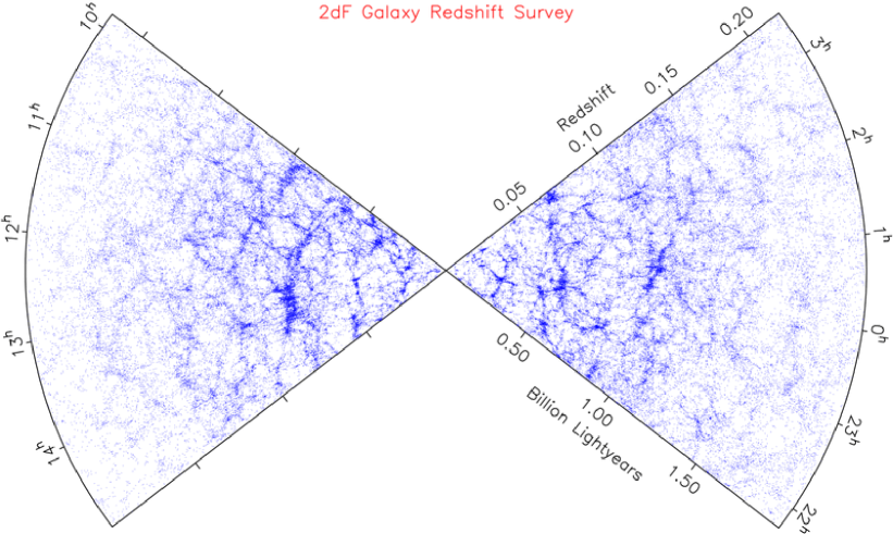
Figure 1.1: The 2-degree Field Galaxy Redshift Survey (2dFGRS) map [41]. The 2dFGRS obtained spectra for 245591 objects, mainly galaxies. Reliable redshifts were obtained for 221414 galaxies. The galaxies cover an area of approximately 1500 square degrees selected from the extended APM Galaxy Survey in three regions: a north galactic pole strip, a south galactic pole strip and random fields scattered around the south galactic pole strip. The figure shows the map of the galaxy distribution produced from the completed survey. The filamentary structure can be qualitatively compared with that predicted by the Cold Dark Matter model with dark energy ($\Lambda$CDM model) (see Fig. 1.2) (Courtesy of the Anglo-Australian Observatory’s 2dFGRS group [1]).

 

 

 

Figure 1.2: These slices show the dark matter distribution in the Universe, based on the Millennium Simulation [208]: the largest N-body simulation carried out thus far (more than $10^{10}$ particles). By zooming in on a massive cluster of galaxies, the slices highlight the morphology of the structure on different scales, and the large dynamic range of the simulation ($10^{5}$ per dimension in 3D). The zoom extends from scales of a few Gpc down to resolved substructures as small as  100 Mpc. The slices through the density field are all 15 Mpc/$h$ thick, with $h=0.71\pm 0.03$ [207]. For each redshift, three panels are displayed. Subsequent panels zoom in by a factor of four with respect to the previous ones. This filamentary structure can be qualitatively compared with that observed by the 2-degree Field Galaxy Redshift Survey (see Fig. 1.1) (Courtesy of the Virgo Consortium for cosmological supercomputer simulations [218]).

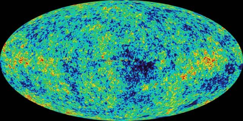
Figure 1.3: CMB temperature anisotropies as seen by the WMAP satellite [26]. The oval shape is a projection to display the whole sky. The temperature anisotropies are found to be of the order of 1 part in $10^{5}$. The background temperature is $T_{0}=2.725\pm 0.002$ K; regions at that temperature are in very light blue. The hottest regions (in red) correspond to $\Delta T=200\mu{\rm K}$. The coldest regions (in very dark blue) correspond to $\Delta T=-200\mu{\rm K}$ (Courtesy of the NASA/WMAP Science Team [223]).

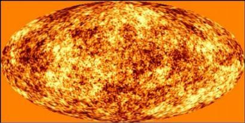
Figure 1.4: Simulation of the CMB temperature anisotropies as seen by the PLANCK satellite. PLANCK will provide a map of the CMB field at all angular resolutions greater than 10 arcminutes and with a temperature resolution of the order of 1 part in $10^{6}$ (ten times better than WMAP) (Courtesy of ESA’s PLANCK mission [171]).

The anisotropies in the CMB temperature $\delta T/T_{0}$ are directly related to the perturbations in the energy density $\delta\rho/\rho_{0}$ at the time of recombination (Sachs-Wolfe effect), whose primarily origin is the stretched quantum fluctuations of one or several scalar fields $\phi_{i}$ that fill the Universe during inflation [112, 191]:

$$\left(\frac{\delta T}{T_{0}}\right)_{k}=-\frac{1}{2}\left(\frac{aH}{k}\right)^{2}\left(\frac{\delta\rho}{\rho_{0}}\right)_{k}\,.$$ (1.1)

The perturbations in the energy density at the time of recombination can in turn be quantified by the gauge-invariant primordial curvature perturbation $\zeta$ [112, 191]:

$$\left(\frac{\delta\rho}{\rho_{0}}\right)_{k}=\frac{2}{5}\left(\frac{k}{aH}\right)^{2}\zeta_{k}\,,$$ (1.2)

which, on flat slices, can be expressed in terms of only the fluctuations in the fields $\phi_{i}$. For instance, in the case of only one scalar field $\varphi$ present during inflation, $\zeta$ [11, 12, 162, 163] is given by

$$\zeta=-H_{\rm inf}\frac{\delta\varphi}{\dot{\varphi}_{0}}\,,$$ (1.3)

where $H_{\rm inf}$ is the global Hubble parameter during inflation. The curvature perturbation $\zeta$ is a convenient quantity to describe the primordial perturbations since it is conserved on superhorizon scales ($k\ll aH_{\rm inf}$), as long as the pressure is a unique function of the energy density [127, 179, 222], and it is well defined even after the scalar fields $\phi_{i}$ have decayed. We will define $\zeta$ in a rigorous way in Chapter 2.

The scalar fields $\phi_{i}$ we have been talking about might or might not have dominated the energy density during inflation and, therefore, driven the inflationary stage prior to the Big-Bang. Our adopted definition for the inflaton field in this thesis will be the light field $\varphi$ that dominates the energy density during inflation and drives the exponential expansion. This field in most cases parameterises the distance along the inflationary trajectories. Until recently, the most widely known and accepted scenario for the origin of the density perturbations identified the inflaton with the scalar field whose fluctuations were responsible for the primordial density perturbations. This scenario, called the inflaton scenario [5, 112, 117, 130], describes very well the properties of $\zeta$, leading to an almost scale invariant power spectrum

$$\mathcal{P}_{\zeta}(k)\equiv A_{\zeta}^{2}\left(\frac{k}{aH_{\rm inf}}\right)^{n_{\zeta}}\,,$$ (1.4)

which is defined by the statistical average

$$\langle\zeta_{{\bf k}_{1}}\zeta_{{\bf k}_{2}}\rangle\equiv\frac{2\pi^{2}}{k^{3}}\delta^{3}({\bf k}_{1}+{\bf k}_{2})\mathcal{P}_{\zeta}(k)\,,$$ (1.5)

calculated over an ensemble of universes. The amplitude $A_{\zeta}$ and spectral index $n_{\zeta}$ in Eq. (1.4) :

$$A_{\zeta} \simeq -\frac{H_{*}}{\sqrt{8\varepsilon}\pi m_{P}}\,,$$ (1.6)

$$n_{\zeta} = 2\eta_{\varphi}-6\varepsilon\,,$$ (1.7)

are functions of the slow-roll parameters

$$\varepsilon \equiv -\left(\frac{\dot{H}_{\rm inf}}{H_{\rm inf}^{2}}\right)_{\ast}\,,$$ (1.8)

$$\eta_{\varphi} \equiv \varepsilon-\frac{\ddot{\varphi}_{0}}{H_{\rm inf}\dot{\varphi}_{0}}\,,$$ (1.9)

that characterize the inflationary behaviour and satisfy the slow-roll conditions $\varepsilon\ll 1$ and $|\eta_{\varphi}|\ll 1$ [111, 112, 130, 185]. The scale of inflation, given by $H_{*}$, is not completely determined in the inflaton scenario by the already measured amplitude $|A_{\zeta}|$ [207], since the slow-roll parameter $\varepsilon$ is unknown (except for the upper bound $\varepsilon\mbox{\raisebox{-3.87495pt}{~{}$\stackrel{{\scriptstyle\mbox{$<$}}}{{\sim}}$~{}}}0.01$ [207]).

The next statistical significant quantity after $\mathcal{P}_{\zeta}(k)$, the bispectrum $B_{\zeta}(k_{1},k_{2},k_{3})$ defined by the statistical average

$$\langle\zeta_{{\bf k}_{1}}\zeta_{{\bf k}_{2}}\zeta_{{\bf k}_{3}}\rangle\equiv(2\pi)^{-3/2}B_{\zeta}(k_{1},k_{2},k_{3})\delta^{3}({\bf k}_{1}+{\bf k}_{2}+{\bf k}_{3})\,,$$ (1.10)

is also well described in the inflaton scenario as its normalisation ${f_{\rm NL}}$, defined by

$$B_{\zeta}(k_{1},k_{2},k_{3})\equiv-\frac{6}{5}{f_{\rm NL}}\left[\frac{2\pi^{2}}{k_{1}^{3}}\mathcal{P}_{\zeta}(k_{1})\frac{2\pi^{2}}{k_{2}^{3}}\mathcal{P}_{\zeta}(k_{2})+{\rm cyclic\ permutations}\right]\,,$$ (1.11)

is suppressed by $\varepsilon$ and $\eta_{\varphi}$ [142] describing a highly gaussian set of perturbations:

$${f_{\rm NL}}=\frac{5}{12}[2\eta_{\varphi}-6\varepsilon-2\epsilon f(k_{1},k_{2},k_{3})]\,.$$ (1.12)

The value of the scale dependent function $f$ in the previous expression lies in the range $0\leq f\leq 5/6$, being precisely determined by the respective wavevector configuration [142].

We make a couple of observations [2, 68, 111, 112, 190] which are valid not only for the inflaton scenario but also for the curvaton one discussed below. First, the amplitude $A_{T}$ of the power spectrum of gravitational waves

$$\mathcal{P}_{T}(k)\equiv A_{T}^{2}\left(\frac{k}{aH_{\rm inf}}\right)^{n_{T}}\,,$$ (1.13)

which is defined by the statistical average

$$\sum_{ij}\langle h^{ij}_{{\bf k}_{1}}h^{ij}_{{\bf k}_{2}}\rangle\equiv\frac{2\pi^{2}}{k^{3}}\delta^{3}({\bf k}_{1}+{\bf k}_{2})\mathcal{P}_{T}(k)\,,$$ (1.14)

where $h_{ij}$ is the tensor perturbation in the perturbed metric tensor, depends only on the scale of inflation (given by $H_{\ast}$):

$$A_{T}\simeq\frac{\sqrt{2}H_{*}}{\pi m_{P}}\,.$$ (1.15)

Second, its tilt $n_{T}$ is a function only of $\varepsilon$:

$$n_{T}=-2\varepsilon\,.$$ (1.16)

In view of our previous discussion about $\mathcal{P}_{\zeta}(k)$, we can write a consistency relation involving $A_{\zeta}$, $A_{T}$, and $n_{T}$, which presents itself as a nice prediction of the inflaton scenario:

$$r_{T\zeta}\equiv\frac{A_{T}^{2}}{A_{\zeta}^{2}}=-8n_{T}\,.$$ (1.17)

Its confirmation, as well as a negative detection of non-gaussianity by both WMAP [102, 103, 223] and PLANCK [103, 171] satellites, would give strong support to the inflaton scenario as the correct framework to understand the origin of the large-scale structure in the Universe. We will discuss in more detail the inflaton scenario in Chapter 2.

An alternative to the inflaton scenario is when the weakly coupled light field $\sigma$, whose fluctuations are responsible for the primordial density perturbations, does not dominate the energy density, and therefore does not drive inflation. This scenario is called the curvaton scenario [138, 139, 159] (see also Refs. [66, 116, 156]), and the field $\sigma$ receives the name curvaton. Introduced in 2002, this scenario describes also very well the properties of $\zeta$, with an almost scale invariant power spectrum $\mathcal{P}_{\zeta}(k)\equiv A_{\zeta}^{2}(k/aH_{\rm inf})^{n_{\zeta}}$ whose spectral index $n_{\zeta}$ written as

$$n_{\zeta}=2\eta_{\sigma}-2\varepsilon\,,$$ (1.18)

is function of $\varepsilon$ and

$$\eta_{\sigma}\equiv\frac{m_{P}^{2}}{V}\frac{\partial^{2}V}{\partial\sigma^{2}_{0}}\approx\frac{m_{\sigma}^{2}}{3H_{\ast}^{2}}\ll 1\,,$$ (1.19)

being $V$ the scalar potential, and whose amplitude $A_{\zeta}$ is given by $H_{\ast}$, the unperturbed component of the curvaton field during inflation $\sigma_{\ast}$, and the fractional global curvaton energy density $\Omega_{\rm dec}\equiv\rho_{\sigma_{0}}/\rho_{\rm total_{0}}$ just before the curvaton decay:

$$A_{\zeta}\simeq\frac{H_{\ast}\Omega_{\rm dec}}{3\pi\sigma_{\ast}}\,.$$ (1.20)

The scale of inflation in the curvaton scenario, given by $H_{\ast}$, does not depend on $\varepsilon$ nor on $\eta_{\sigma}$, instead it depends on the free parameters $\sigma_{*}$ and $\Omega_{\rm dec}$. A consequence from the previous expression is that there is no analogous to the consistency relation [c.f. Eq. (1.17)] for the curvaton scenario. However, there are distinctive non-gaussian signatures that can allow us to distinguish this model from other scenarios for the origin of the large-scale structure in the Universe (see below) [14, 17, 126, 131, 138]. The curvaton scenario will be studied in detail in Chapter 2.

Perhaps the main motivation for the introduction of the curvaton scenario is that it liberates the inflaton field from the generation of the primordial perturbations [49, 160, 161]. This is particularly good from the particle physics point of view since the intrinsic difficulty at embedding the inflaton scenario in a particle physics model is greatly alleviated. Indeed, in the inflaton scenario, the energy scale of inflation is likely to be quite high ($H_{*}\mbox{\raisebox{-3.87495pt}{~{}$\stackrel{{\scriptstyle\mbox{$<$}}}{{\sim}}$~{}}}10^{14}$ GeV) [123] in order to produce the required level of primordial perturbations $|A_{\zeta}|\approx 5\times 10^{-5}$ [207]. This makes very difficult the identification of the inflaton field with one of the scalar fields present in the supersymmetry (SUSY) breaking sector or with one of the Minimal Supersymmetric Standard Model (MSSM) flat directions. This is because the characteristic SUSY energy scale, which depends on the symmetry breaking scheme, goes typically from $H_{*}\sim 10^{-2}$ GeV to $H_{*}\sim 10^{5}$ GeV [125, 126]. In contrast, in the curvaton scenario, the energy scale has to be much lower, satisfying $H_{*}\mbox{\raisebox{-3.87495pt}{~{}$\stackrel{{\scriptstyle\mbox{$<$}}}{{\sim}}$~{}}}10^{12}$ GeV [138, 139, 159], so that the inflaton field does not contribute to the curvature perturbation [c.f. Eq. (1.6)]. The last bound can be taken as an anti-smoking gun for the curvaton scenario because a positive gravitational wave signal would require $H_{*}\mbox{\raisebox{-3.87495pt}{~{}$\stackrel{{\scriptstyle\mbox{$>$}}}{{\sim}}$~{}}}10^{12}$ GeV [85, 94, 95, 201, 202, 205], ruling out the curvaton as the source of primordial density fluctuations. Some people can see this as a bad feature of the scenario in question as it sends an unpromising message to all those who are making big efforts to detect gravitational waves. However, as described in Ref. [170], the curvaton scenario may well be consistent with detectable gravitational waves as far as the inflaton is a ‘heavy’ field ($m_{\varphi}\mbox{\raisebox{-3.87495pt}{~{}$\stackrel{{\scriptstyle\mbox{$>$}}}{{\sim}}$~{}}}H_{\ast}$), violating this way the slow-roll condition $|\eta_{\varphi}|\ll 1\$, and suppressing the amplitude of the curvature perturbation produced by the inflaton itself.

One of our main concerns in this thesis is the possibility to accommodate low-scale inflation in the curvaton scenario. Unfortunately, even when the energy scale may in principle be greatly reduced compared to the inflaton scenario, the simplest curvaton model still requires a quite high inflationary energy scale satisfying $H_{\ast}>10^{7}$ GeV [126]. This of course makes impossible the embedding of the inflaton field within the framework of a SUSY particle physics model. In Chapters 3 and 4 we explore two modifications to the curvaton model which can instead allow inflation at a low scale [51, 149, 175, 189]. In the first modification [51] the end of a second (thermal) inflationary stage [108, 136, 137], driven by the rolling of a flaton field $\chi$ coupled to the curvaton, makes the curvaton mass $m_{\sigma}$ increase suddenly at some moment after the end of inflation but before the onset of the curvaton oscillations. This proposal can work but not in a completely natural way. Nevertheless, we show that inflation with $H_{\ast}$ as low as 1 TeV or lower is possible to attain. In the second modification [175, 189] the increment in $m_{\sigma}$ at the end of the thermal inflation era is so huge that the decay rate overtakes the Hubble parameter and the curvaton field decays immediately. The advantage of this second modification is that low scale inflation is achieved for more natural values in the relevant parameter space.

Aside from the previously introduced theoretical aspects of the origin of the large-scale structure in the Universe, we also study some of its statistical aspects. Conversely to the inflaton scenario [c.f. Eq. (1.12)], $\zeta$ in the simplest curvaton model may present a sizable non-gaussian component if the curvaton does not dominate the energy density before decaying [14, 17, 131, 138]. More specifically, according to the expression

$${f_{\rm NL}}=\frac{5}{3}+\frac{5}{6}r-\frac{5}{4r}\,,$$ (1.21)

which is valid in the curvaton scenario, $|{f_{\rm NL}}|\gg 1$ is obtained if $r$ is very small. In the previous expression $r$ is defined by

$$r\equiv\frac{3\rho_{\sigma_{0}}}{4\rho_{r_{0}}+3\rho_{\sigma_{0}}}\,,$$ (1.22)

and is evaluated just before the curvaton decay (being $\rho_{r}$ the global radiation energy density). This is of extreme importance since the next WMAP data release [102, 103, 223], or in its defect the future PLANCK satellite data [103, 171], will either detect non-gaussianity or put strong constraints on ${f_{\rm NL}}$, offering the possibility of successfully discriminating among the different inflaton and curvaton models. The current constraint on ${f_{\rm NL}}$, according to the first-year WMAP data, is $|{f_{\rm NL}}|\mbox{\raisebox{-3.87495pt}{~{}$\stackrel{{\scriptstyle\mbox{$<$}}}{{\sim}}$~{}}}10^{2}$ [102]. The next data release is expected to lower this bound by one order of magnitude or so [103].

The non-linearity parameter ${f_{\rm NL}}$, if independent of position, is closely related to the second-order curvature perturbation $\zeta_{2}$ defined by

$$\zeta({\bf x}) \equiv \zeta_{1}({\bf x})+\frac{1}{2}\zeta_{2}({\bf x})$$ (1.23)

$$\equiv \zeta_{g}({\bf x})-\frac{3}{5}{f_{\rm NL}}(\zeta_{g}^{2}({\bf x})-\langle\zeta_{g}^{2}\rangle)\,,$$

where $\zeta_{g}$ is gaussian with $\langle\zeta_{g}\rangle=0$. In connection with this issue we point out that several conserved and/or gauge invariant quantities described as the second-order curvature perturbation have been given in the literature [3, 140, 142, 145]. In Chapter 5 we revisit various scenarios for the generation of second-order non-gaussianity in $\zeta$, employing for the first time a unified notation and focusing on $f_{\rm NL}$ [131]. When $\zeta$ first appears a few Hubble times after horizon exit, $|f_{\rm NL}|$ is much less than $1$ and is, therefore, negligible. Thereafter $\zeta$ (and hence $f_{\rm NL}$) is conserved as long as the pressure is a unique function of the energy density (adiabatic pressure) [127, 179, 222]. Non-adiabatic pressure comes presumably only from the effect of fields, other than the one pointing along the inflationary trajectory, which are light during inflation (light non-inflaton fields) [23, 77]. Our expectation is that, although during single-component inflation ${f_{\rm NL}}$ is constant, multi-component inflation might generate $|f_{\rm NL}|\sim 1$ or bigger. We mention some recent proposals where non-gaussianity can be generated during the preheating stage following inflation [60, 61, 62], and conjecture that preheating can affect ${f_{\rm NL}}$ only in atypical scenarios where it involves light non-inflaton fields [8, 24, 25, 62, 100]. We also study the curvaton scenario and derive Eq. (1.21), showing that the simplest model typically gives ${f_{\rm NL}}\ll-1$ or ${f_{\rm NL}}=+5/4$. The inhomogeneous reheating scenario [53, 54, 97] (see also Refs. [65, 148, 150, 151, 216, 224]), where $\zeta$ is generated by the inhomogeneities in the inflaton decay rate during reheating, is quickly reviewed showing that it can give a wide range of values for ${f_{\rm NL}}$ [216, 224]. One important conclusion from this chapter is that it will be crucial to calculate the precise observational limit on ${f_{\rm NL}}$ using second order theory in case that, unless there is a detection, observation could eventually provide a limit $|{f_{\rm NL}}|\mbox{\raisebox{-3.87495pt}{~{}$\stackrel{{\scriptstyle\mbox{$<$}}}{{\sim}}$~{}}}1$ [103].

A new and interesting proposal is the extension to second order of the $\delta N$ formalism [196] (see also Refs. [210, 211]), used initially to calculate $\zeta$ at first order and the spectral index in multi-component slow-roll models of inflation [196]. In this formalism $\zeta(t,{\bf x})$ is expressed as the perturbation in the amount of expansion

$$N(t,{\bf x})\equiv\ln\left[\frac{\tilde{a}(t,{\bf x})}{a(t_{\rm in})}\right]\,,$$ (1.24)

from an initially flat slice at time $t_{in}$ to a final slice of uniform energy density at time $t$:

$$\zeta(t,{\bf x})=\delta N\equiv N(t,{\bf x})-N_{0}(t)\,.$$ (1.25)

Here

$$N_{0}(t)\equiv\ln\left[\frac{a(t)}{a(t_{\rm in})}\right]\,,$$ (1.26)

is the unperturbed amount of expansion, and $\tilde{a}(t,{\bf x})$ is the local expansion parameter. Thus, $\zeta$ up to second order is given by

$$\zeta(t,{\bf x})=\sum_{i}N_{,i}(t)\delta\phi_{i}+\frac{1}{2}\sum_{ij}N_{,ij}(t)\delta\phi_{i}\delta\phi_{j}\,,$$ (1.27)

where

$$N_{,i} = \frac{\partial N}{\partial\phi_{i_{0}}}\,,$$ (1.28)

$$N_{,ij} = \frac{\partial^{2}N}{\partial\phi_{i_{0}}\partial\phi_{j_{0}}}\,,$$ (1.29)

and the fields $\phi_{i}$, evaluated a few Hubble times after horizon exit, are those relevant for the generation of $\zeta$. In view of Eq. (1.23), this presents as a powerful method to calculate ${f_{\rm NL}}$ in any multi-component slow-roll inflationary model for the generation of $\zeta$ [132]. In Chapter 6 we give for the first time this formalism, which allows us to extract all the stochastic properties of $\zeta$ if the initial field perturbations are gaussian. The elegance and power of this method lies in the fact that the calculation requires only the knowledge of the evolution of some family of unperturbed universes. The following formula is given for ${f_{\rm NL}}$ in terms of $N(t,\phi_{i_{0}})$ and its derivatives [32, 132]:

$$-\frac{3}{5}{f_{\rm NL}}=\frac{\sum_{ij}{N_{,i}}{N_{,j}}{N_{,ij}}}{2\left[\sum_{i}{N_{,i}}^{2}\right]^{2}}+\ln(kL)\frac{A_{\zeta}^{2}}{2}\frac{\sum_{ijk}{N_{,ij}}N_{,jk}N_{,ki}}{\left[\sum_{i}{N_{,i}}^{2}\right]^{3}}\,,$$ (1.30)

where $k^{-1}$ is a typical cosmological scale and $L$ is the size of the region within which the stochastic properties are specified, so that $\ln(kL)\sim 1$. We apply the above formula to the Kadota and Stewart modular inflation model [90, 91], the curvaton scenario [138, 139, 159], and the multi-component ‘hybrid’ inflation model of Enqvist and V$\ddot{{\rm a}}$ihk$\ddot{{\rm o}}$nen [67]. The relation of this formula to cosmological perturbation theory is also explained.

The conclusions of this thesis are drawn in Chapter 7.

Chapter 2 Two mechanisms for the origin of the large-scale structure

2.1 Introduction

In the standard inflationary scenario [5, 112, 117, 130] a single scalar field, named the inflaton, is responsible for the solution of the horizon, flatness, and unwanted relics problems, as well as for the origin of the large scale structure seen in the observable Universe. This double mission for the inflaton field imposes strong constraints on the parameters of the inflationary models, leading to big intrinsic difficulties at building successful and realistic models of inflation [112, 130]. To rescue the well motivated inflationary models that fail at generating the required level of primordial perturbations [49], the inflaton field is left in charge of driving inflation only. The other task, the generation of the primordial perturbations, is assigned to a weakly coupled light field $\sigma$ different from the inflaton. This is the curvaton scenario [138, 139, 159] (see also Refs. [66, 116, 156]), where the original curvature perturbation $\zeta_{\sigma}$, associated to and produced by $\sigma$ during inflation, is gradually transformed into the total curvature perturbation $\zeta$ . The conversion process starts during the radiation dominated epoch that follows the reheating stage produced by the inflaton decay.

This chapter will give some preliminary definitions and basic facts about the inflaton and the curvaton scenarios, such as the first-order perturbations in the metric, the precise definition of $\zeta$, the slow-roll conditions, the characteristics of the spectrum of $\zeta$ in both the inflaton and the curvaton scenarios, and the spectrum of gravitational waves and the consequences derived from its possible detection. Having this information at hand, it will be easier to follow the main discussions of this thesis that are exposed in Chapters 3 to 6.

2.2 Metric perturbations and the primordial curvature perturbation $\zeta$

Our observable expanding Universe is well described as homogeneous and isotropic, down to scales of order of tens of Megaparsecs. The FRW line element

$$ds^{2}=-dt^{2}+a^{2}(t)\left(\frac{dr^{2}}{1-\kappa r^{2}}+r^{2}d\theta^{2}+r^{2}\sin^{2}\theta d\phi^{2}\right)\,,$$ (2.1)

describes such an Universe [72, 186, 187, 188, 220], assuming that the galaxies are always at the same comoving spherical coordinates $r$, $\theta$, and $\phi$, and that the intergalactic space is continually increasing with time due to the expansion parameter (scale factor) $a(t)$. The proper time, once synchronized in all the galaxies, runs at the same rate everywhere, so the metric is well described by a global cosmic time $t$. Finally, the topology of the Universe can be classified by the parameter $\kappa$ as closed ($\kappa>0$), open ($\kappa=0$), or flat ($\kappa<0$), according to whether the space is finite but unbounded, infinite with certain curvature, or infinite but strictly flat a la Minkowski . The inflationary stage however shrinks the comoving horizon so rapidly that the present Universe looks so extremely flat. This makes the parameter $\kappa$ be completely irrelevant when going back in time, so that we can safely discard it when studying the inflationary and early Universe processes. Thus, and switching to cartesian coordinates $x^{i}$ and conformal time $\eta$ defined by $d\eta\equiv dt/a$, the FRW line element looks

$$ds^{2}=a^{2}(\eta)\left(-d\eta^{2}+\delta_{ij}dx^{i}dx^{j}\right)\,.$$ (2.2)

2.2.1 First-order perturbations in the FRW line element: classification and number of degrees of freedom

The homogeneity and isotropy assumptions make a good description of the Universe, but they are not in any case perfect conditions. The observed galaxy distribution and the temperature fluctuations in the CMB (see Figs. 1.1 - 1.4) reveal the importance of modifying the FRW line element so that it accounts for the small deviations from homogeneity and isotropy required to correctly describe such large-scale structures. The introduction of small inhomogeneities in the FRW line element, and the truncation at first-order of the perturbed Einstein equations, are well justified since the galaxy density contrast $\delta\rho/\rho_{0}$ and the CMB temperature anisotropies $\delta T/T_{0}$ are observed to be of order $10^{-5}$ [26, 104, 169]. In consequence, considering only scalar degrees of freedom, the most generic first-order perturbed line element reads [11, 96, 143, 162, 163, 185, 195]

$$ds^{2}=a^{2}(\eta)\left[-(1+2\phi_{G})d\eta^{2}+2\,\partial_{i}B\,d\eta dx^{i}+((1-2\psi)\delta_{ij}+D_{ij}E)dx^{i}dx^{j}\right]\,,$$ (2.3)

where $D_{ij}\equiv\partial_{i}\partial_{j}-(1/3)\delta_{ij}\nabla^{2}$, and $\phi_{G}$, $B$, $\psi$, and $E$ are scalar quantities.

The peculiar form of the perturbed line element in Eq. (2.3), as well as the right number of scalar degrees of freedom in that expression, are justified as follows:

• The full perturbed metric tensor is generically described by scalar, vector, and tensor perturbations.

• The total number of degrees of freedom for a symmetric tensor in an $(n+1)$-dimensional spacetime is $(n+2)(n+1)/2$.

• The $g_{00}$ entry can be written as $-(1+2\phi_{G})$, where $\phi_{G}$ corresponds to a purely scalar perturbation (1 scalar degree of freedom).

• The $g_{0i}$ entries can be parameterised by $B_{i}\equiv\partial_{i}B+\upsilon_{i}$, where $\vec{\nabla}\cdot\vec{\upsilon}=0$. The term $\partial_{i}B$ corresponds to a purely scalar perturbation (1 scalar degree of freedom). The term $\upsilon_{i}$ corresponds to a purely vector perturbation ($n-1$ vector degrees of freedom because of the $\vec{\nabla}\cdot\vec{\upsilon}=0$ constraint).

• The $g_{ij}$ entries can be written as $(1-2\psi)\delta_{ij}+\Pi_{ij}$, where $\psi$ is a purely scalar perturbation (1 scalar degree of freedom) that accounts for the trace of $g_{ij}$, and $\Pi_{ij}$ is a symmetric traceless tensor.

• $\Pi_{ij}=\Pi_{ij}^{S}+\Pi_{ij}^{V}+\Pi_{ij}^{T}$ is expressed in terms of a purely scalar perturbation (encoded in $\Pi_{ij}^{S}$), a purely vector perturbation (encoded in $\Pi_{ij}^{V}$), and a purely tensor perturbation (encoded in $\Pi_{ij}^{T}$).

• $\Pi_{ij}^{S}$ can be written as $D_{ij}E$ because it is a symmetric traceless tensor corresponding to the purely scalar perturbation $E$ (1 scalar degree of freedom).

• $\Pi_{ij}^{V}$ can be written as $(\partial_{i}\Pi_{j}+\partial_{j}\Pi_{i})/2$, where $\Pi_{i}$ is a purely vector perturbation satisfying $\vec{\nabla}\cdot\vec{\Pi}=0$ ($n-1$ vector degrees of freedom).

• $\Pi_{ij}^{T}$ corresponds to a purely tensor perturbation such that $\partial_{i}\Pi_{ij}^{T}=0$. Considering the previous three items, and the fact that the number of degrees of freedom coming from a traceless symmetric tensor in an $n$-dimensional space is $(n+1)n/2-1$, the number of tensor degrees of freedom is $(n-2)(n+1)/2$.

• The total number of scalar degrees of freedom (4), vector degrees of freedom ($2(n-1)$), and tensor degrees of freedom ($(n-2)(n+1)/2$), add up to reproduce the total number of degrees of freedom of the metric tensor $g_{\mu\nu}$ given in the second item: $(n+2)(n+1)/2$.

Two very important facts follow from the first-order perturbed Einstein equations [11, 96, 143, 163]. First, at first order the vector perturbations are decoupled from the scalar perturbations being anyway usually neglected due to their rapid decrease with time. Second, the tensor perturbations at first order also decouple from their scalar counterparts. These two facts, along with the parameterisation of the metric tensor discussed in the above items, justify the use of the Eq. (2.3) as the most generic first-order metric perturbed line element that describes the energy density (scalar) perturbations in the FRW spacetime.

2.2.2 The curvature perturbation $\psi$ and its non-invariance under infinitesimal coordinate transformations

In the perturbed line element of Eq. (2.3), $\psi$ represents the intrinsic spatial curvature ${}^{(3)}R$ on hypersurfaces of constant conformal time $\eta$ [11]:

$${}^{(3)}R=\frac{4}{a^{2}}\nabla^{2}\psi\,,$$ (2.4)

where the operator $\nabla^{2}$ is the comoving Laplacian operator. For this reason the quantity $\psi$ is usually referred to as the curvature perturbation. The curvature perturbation $\psi$, as well as the other scalar perturbations $\phi_{G}$, $B$, and $E$, are however not invariant under a coordinate transformation. Indeed, from the most general infinitesimal coordinate transformation

$$\eta \rightarrow \eta+\xi(x^{\mu})\,,$$ (2.5)

$$x_{i} \rightarrow x_{i}+\partial_{i}\beta(x^{\mu})\,,$$ (2.6)

the scalar perturbations $\phi_{G}$, $B$, $\psi$, and $E$ transform as [11]

$$\phi_{G} \rightarrow \phi_{G}-\xi^{\prime}-\mathcal{H}\xi\,,$$ (2.7)

$$B \rightarrow B+\xi-\beta^{\prime}\,,$$ (2.8)

$$\psi \rightarrow \psi+\frac{1}{3}\nabla^{2}\beta+\mathcal{H}\xi\,,$$ (2.9)

$$E \rightarrow E-2\beta\,,$$ (2.10)

where a prime means derivation with respect to the conformal time $\eta$, and $\mathcal{H}$ is the global conformal Hubble parameter defined by $\mathcal{H}\equiv a^{\prime}/a$. The above transformation rules are under the physical proviso that the perturbed line element $ds^{2}$ in Eq. (2.3) should remain invariant.

The parameters $\xi$ and $\beta$ that give account of the infinitesimal coordinate transformation in Eqs. (2.5) and (2.6) can be adjusted (fixing the slicing and the threading) so that two of the four scalar perturbations in Eqs. (2.7) to (2.10) vanish. The longitudinal gauge, for instance, corresponds to choose $B$ and $E$ equal to zero. In this specific gauge the gravitational potential $\phi_{G}$ becomes equal to the curvature perturbation $\psi$ up to first order [96, 143, 162, 163, 185] as long as the considered fluid is described by a perfect isotropic stress, examples of such a fluid being the inflaton and/or the curvaton fields. All of this leads us to say with confidence that the curvature perturbation $\psi$ really represents the effect of the inhomogeneities in the FRW spacetime and it is, therefore, the quantity to study.

2.2.3 The gauge-invariant curvature perturbation $\zeta$

To parameterise adequately the inhomogeneities in the FRW spacetime, we need a quantity invariant under the coordinate (gauge) transformations in Eqs. (2.5) and (2.6). This is not completely possible to do, but we may define a quantity which is invariant under transformations in time only. This is done taking into account that, for any scalar quantity $f(x^{\mu})$ different to $\phi_{G}$, $B$, $\psi$, and $E$, the transformation law in the associated perturbation $\delta f(x^{\mu})$ is given by

$$\delta f\rightarrow\delta f-f_{0}^{\prime}\xi\,.$$ (2.11)

The first gauge invariant quantity that we may define is that which represents the curvature perturbation $\psi$ in the comoving slices, defined them as the constant time hypersurfaces where there is no flux of energy. Considering the inflaton field $\varphi$, the comoving slices coincide with those where $\varphi$ is uniform ($\delta\varphi_{\rm com}=0$) [96, 127, 163, 222] so that the time translation $\xi_{\rm com}(x^{\mu})$ required to go from a generic slice to the comoving slice is:

$$\xi_{\rm com}=\frac{1}{\varphi_{0}^{\prime}}[\delta\varphi-\delta\varphi_{\rm com}]=\frac{\delta\varphi}{\varphi_{0}^{\prime}}\,.$$ (2.12)

Therefore the comoving curvature perturbation $\psi_{\rm com}$, denoted from now on as $-\zeta$, is written in terms of $\psi$ and $\varphi$ in the generic slice as

$$\zeta = -\psi-\mathcal{H}\xi_{\rm com}$$ (2.13)

$$= -\psi-\mathcal{H}\frac{\delta\varphi}{\varphi_{0}^{\prime}}\,.$$

The overall minus sign is just a convention, chosen in this thesis to match the agreed definition of $\zeta$ by most of the authors.

The second gauge invariant quantity that we may define represents the curvature perturbation $\psi$ in the slices of uniform energy density. Again, and following the same steps as before, we have to consider the infinitesimal time translation $\xi_{\rm uni}(x^{\mu})$ required to go from a generic slice to the uniform energy density slice where $\delta\rho_{\rm uni}=0$:

$$\xi_{\rm uni}=\frac{1}{\rho_{0}^{\prime}}[\delta\rho-\delta\rho_{\rm uni}]=\frac{\delta\rho}{\rho_{0}^{\prime}}\,.$$ (2.14)

Thus, the curvature perturbation in the uniform density slice $\psi_{\rm uni}$, denoted from now on as $-\zeta$, is given by

$$\zeta = -\psi-\mathcal{H}\xi_{\rm uni}$$ (2.15)

$$= -\psi-\mathcal{H}\frac{\delta\rho}{\rho_{0}^{\prime}}\,.$$

We have chosen to denote both the comoving and the uniform density slice curvature perturbations with the same letter $\zeta$ because they are equivalent on superhorizon scales ($k\ll aH_{\rm inf}$) [11]. The superhorizon scale region is of great importance because $\zeta$ is conserved in that region if the adiabatic condition, described below, is satisfied. In addition, at superhorizon scales $\zeta$ becomes truly gauge-invariant because the contribution of $\beta$ in Eq. (2.9) gets suppressed by the spatial derivatives, so that $\psi$ does not depend on the changes in the threading.

The conservation of $\zeta$ is guaranteed as long as the pressure $P$ is a unique function of the energy density $\rho$ (the adiabatic condition). The last statement follows from the local energy conservation equation in the uniform density slicing at large scales [127, 179, 222]:

$$\dot{\rho}(t)=-3(H+\dot{\zeta})[\rho(t)+P(t,{\bf x})]\,.$$ (2.16)

If $P$ satisfies the adiabatic condition then it becomes spatially uniform ($\zeta=\langle\zeta\rangle$), and so does $\dot{\zeta}$. As a result

$$\dot{\zeta}=0\,,$$ (2.17)

because

$$\dot{\zeta}=\langle\dot{\zeta}\rangle=\frac{d}{dt}\langle\zeta\rangle=0\,.$$ (2.18)

If $P$ does not satisfy the adiabatic condition, i.e. if it has a non-adiabatic component $P_{\rm nad}$, Eq. (2.16) implies

$$\dot{\zeta}=-\frac{H}{\rho_{0}+P_{0}}\delta P_{\rm nad}\,.$$ (2.19)

The curvaton scenario is one example where the existence of a non-adiabatic pressure perturbation makes $\zeta$ evolve from the negligible curvature perturbation produced by the inflaton to the right value observed today. The non-adiabatic pressure perturbation is, in this case, the result of the presence of two weakly interacting fluids, the curvaton matter fluid and the radiation fluid, in the period that follows the inflaton decay and reheating.

2.3 Inflation and its effect on the spectrum of perturbations of a non-dominating massless scalar field during a de Sitter stage

Any period in the history of the Universe during which the expansion is accelerated is denominated as inflationary [5, 79, 112, 117, 130]. The inflationary stage prior to the Hot Big-Bang has the nice property to stretch the quantum fluctuations of the scalar fields living in the FRW spacetime [12, 80, 84, 118, 162, 163, 185, 210], so that they become classical [4, 78, 81, 122, 124] and almost constant, sourcing the primordial density inhomogeneities responsible for the presently observed large-scale structure. The amplitude of the spectrum of the classical field perturbations (for light fields) is generically the same for all kinds of quasi de Sitter models. However, the spectral index is written down in a certain way for fields that dominate the energy density and in another way for fields that do not. In this section we will describe inflation, paying special attention to the constraint imposed by it on the slow-roll parameter $\varepsilon$, and review the properties of the power spectrum of perturbations of a massless scalar field during a de Sitter stage, characterized the latter by a constant Hubble parameter $H_{\rm inf}=H_{\ast}$ during inflation.

2.3.1 Inflation

Inflation can be rigorously defined as the period when the global expansion parameter $a$ satisfies the condition

$$\ddot{a}>0\,.$$ (2.20)

Such a condition translates into a definite requirement on the global Hubble parameter during inflation $H_{\rm inf}$. From the definition of $H_{\rm inf}$ in terms of $a$, which can be written alternatively as the following evolution equation:

$$a(t)=a_{\rm ini}\exp\left(\int_{t_{\rm ini}}^{t}H_{\rm inf}dt\right)\,,$$ (2.21)

being $a_{\rm ini}$ the expansion parameter at some time $t_{\rm ini}$, the inflationary condition in Eq. (2.20) is satisfied while

$$\dot{H}_{\rm inf}>-H^{2}_{\rm inf}\,.$$ (2.22)

The last expression reduces to an upper bound on the slow-roll parameter $\varepsilon$ defined in Eq. (1.8):

$$\varepsilon\equiv-\left(\frac{\dot{H}_{\rm inf}}{H^{2}_{\rm inf}}\right)_{\ast}<1\,.$$ (2.23)

Inflation is held as long as $\varepsilon<1$, being one possibility when $H_{\rm inf}$ is constant in time. This scenario is commonly recognized as the de Sitter stage, and it will be useful at studying the spectrum of perturbations of a massless scalar field. Other possibilities correspond to nonvanishing values for $\dot{H}_{\rm inf}$, being the quasi de Sitter case ($\varepsilon\ll 1$) the most popular. Indeed, the quasi de Sitter stage supplemented by the condition $|\eta_{\varphi}|\ll 1$, being $\eta_{\varphi}$ the slow-roll parameter defined in Eq. (1.9), is what is known as slow-roll inflation. This variety of inflation will be discussed in Subsection 2.5.1. Meanwhile in the following subsection, we will study the fluctuations of a non-dominating massless scalar field during a de Sitter stage. Later on we will generalise these results to the fluctuations of non-dominating and dominating massive scalar fields in a quasi de Sitter stage.

2.3.2 Spectrum of perturbations of a non-dominating massless scalar field during a de Sitter stage

In this subsection we will consider the effects of a de Sitter inflationary stage on the fluctuations of a massless scalar field that does not dominate the energy density. Let’s call this field $\phi$. During inflation, and before horizon exit, the fluctuations in $\phi$ can still be regarded as quantum operators. If we further assume that $\phi$ is almost a non-interacting field, we can write down the field perturbation operator $\delta\hat{\phi}({\bf x},t)$ in terms of the usual creation and annihilation operators $\hat{a}^{\dagger}_{\bf k}$ and $\hat{a}_{\bf k}$:

$$\delta\hat{\phi}({\bf x},t)=\int\frac{d^{3}k}{(2\pi)^{3/2}}\exp(i{\bf k\cdot x})\delta\hat{\phi}_{\bf k}(t)\,,$$ (2.24)

where

$$\delta\hat{\phi}_{\bf k}(t)\equiv\omega_{k}(t)\hat{a}_{\bf k}+\omega_{k}^{\ast}(t)\hat{a}^{\dagger}_{\bf-k}\,.$$ (2.25)

As it was discussed in the introduction of this thesis, the properties of the primordial curvature perturbation $\zeta$ are specified by the spectrum $\mathcal{P}_{\zeta}(k)$, which is defined by the statistical average $\langle\zeta_{{\bf k}_{1}}\zeta_{{\bf k}_{2}}\rangle$ over an ensemble of universes. The same definition can be applied for the perturbations in $\phi$, so that the only information we need to know to calculate $\mathcal{P}_{\delta\phi}(k)$ is the quantum state of the Universe during inflation, being the most reasonable choice the vacuum state. Since the universes in the ensemble are all in the vacuum state during inflation, the statistical average $\langle\delta\phi_{{\bf k}_{1}}\delta\phi_{{\bf k}_{2}}\rangle$ is now very easy to calculate corresponding to the expectation value $\langle 0|\delta\hat{\phi}_{{\bf k}_{1}}\delta\hat{\phi}_{{\bf k}_{2}}|0\rangle$. It is straightforward then to recognize that the spectrum $\mathcal{P}_{\delta\phi}(k)$ of the $\delta\phi$ perturbations, defined by

$$\langle\delta\phi_{{\bf k}_{1}}\delta\phi_{{\bf k}_{2}}\rangle\equiv\frac{2\pi^{2}}{k^{3}}\delta^{3}({\bf k}_{1}+{\bf k}_{2})\mathcal{P}_{\delta\phi}(k)\,,$$ (2.26)

is given by the simple formula

$$\mathcal{P}_{\delta\phi}(k)=\frac{k^{3}}{2\pi^{2}}|\omega_{k}|^{2}\,.$$ (2.27)

To calculate $|\omega_{k}|$ we need to solve the Klein-Gordon equation for the fluctuations in $\phi$. The usual Klein-Gordon equation

$$\ddot{\omega}_{k}+3H_{\ast}\dot{\omega}_{k}+\frac{k^{2}}{a^{2}}\omega_{k}=0\,,$$ (2.28)

is only applicable if the inflaton field (that which dominates the energy density) is unable to generate significant primordial perturbations. That guarantees that the line element in Eq. (2.2) is not modified by any scalar perturbation as $\phi$ is assumed not to dominate the energy density during inflation. As a consequence, the usual structure of the Klein-Gordon equation is unmodified.

Eq. (2.28) is easily solved by making the following change of variables:

$$\omega_{k}\equiv\frac{\lambda_{k}}{a}\,,$$ (2.29)

and going to conformal time where the expansion parameter in a de Sitter stage ($H_{\rm inf}$ being constant)

$$a(t)=a_{\rm ini}\exp[H_{\ast}(t-t_{\rm ini})]\,,$$ (2.30)

is given by

$$a(\eta)=-\frac{1}{H_{\ast}\eta}\,,$$ (2.31)

with conformal time $\eta$ taking negative values. Thus, the Klein-Gordon equation in Eq. (2.28) reduces to

$$\lambda_{k}^{\prime\prime}+\left(k^{2}-\frac{2}{\eta^{2}}\right)\lambda_{k}=0\,,$$ (2.32)

whose exact solution is

$$\lambda_{k}=\frac{\exp(-ik\eta)}{\sqrt{2k}}\left(1-\frac{i}{k\eta}\right)\,.$$ (2.33)

The reader might worry about the fact that Eq. (2.33) is valid up to a multiplicative constant. To solve this ambiguity we note that in the subhorizon regime ($k\gg aH_{\rm inf}$) Eq. (2.32) reproduces the Klein-Gordon equation for a massless scalar field in Minkowski spacetime. The solution for $\lambda_{k}$ in Eq. (2.33) satisfies the Bunch and Davies normalisation [30, 37] on subhorizon scales, so that no integration constant should amplify it.

The subhorizon regime is useful in the sense that we can find the adequate solution and normalisation for $\lambda_{k}$. However, the superhorizon regime ($k\ll aH_{\rm inf}$) is much more interesting because $\zeta$ defined in that regime is truly gauge invariant and conserved as long as the pressure satisfies the adiabatic condition. From Eqs. (2.29), (2.31), and (2.33), the magnitude of the mode function $\omega_{k}$ for superhorizon scales turns out to be constant and it is given by

$$|\omega_{k}|\approx\frac{H_{\ast}}{\sqrt{2k^{3}}}\,.$$ (2.34)

The latter expression allows us to obtain the spectrum of perturbations in $\phi$, given by Eq. (2.27):

$$\mathcal{P}_{\delta\phi}(k)\approx\left(\frac{H_{\ast}}{2\pi}\right)^{2}\,.$$ (2.35)

As we can see, the spectrum $\mathcal{P}_{\delta\phi}(k)$ of the perturbations of a massless scalar field $\phi$ in a de Sitter stage is constant and scale invariant. We will see later on that the previous amplitude is generically the same for any kind of quasi de Sitter model as far as we deal with light fields. A possible scale dependence will arise if the field under consideration has a finite mass and/or if the inflationary stage is not completely de Sitter ($\dot{H}_{\rm inf}\neq 0$).

2.4 The curvaton scenario: an example of a non-dominating light scalar field during a quasi de Sitter stage

In the previous section we described the spectrum of perturbations of a non-dominating massless scalar field during an inflationary period with $H_{\rm inf}$ being constant (de Sitter stage). Now we move a step ahead considering a non-dominating scalar field $\sigma$ whose mass $m_{\sigma}$ satisfies $m_{\sigma}\ll H_{\ast}$ (light field), during an inflationary period where the Hubble parameter $H_{\rm inf}$ is not constant but evolves slowly satisfying the condition $-\dot{H}_{\rm inf}/H^{2}_{\rm inf}\ll 1$ so that $\varepsilon\ll 1$ (quasi de Sitter stage). We will see that the introduction of a slowly varying $H_{\rm inf}$ and a small mass $m_{\sigma}$ for the field $\sigma$ results in a small scale dependence for $\mathcal{P}_{\delta\sigma}(k)$ which is parameterised by $\varepsilon$ and $\eta_{\sigma}\equiv m_{\sigma}^{2}/3H_{\ast}^{2}$. The amplitude of $\mathcal{P}_{\delta\sigma}(k)$ will turn out to be the same as that for a non-dominating massless scalar field in a de Sitter stage, which was the case described in Subsection 2.3.2. This example will help us to understand the properties of the curvature perturbation produced in one of the most satisfying models proposed to explain the origin of the large-scale structure in the Universe: the curvaton scenario.

2.4.1 Spectrum of perturbations of a non-dominating light scalar field during a quasi de Sitter stage

The calculation of the spectrum of perturbations of a non-dominating light scalar field $\sigma$ during a quasi de Sitter stage closely resembles that done in Subsection 2.3.2. We will now have to consider the mass $m_{\sigma}$ of $\sigma$ and the running of $H_{\rm inf}$ given by the slow-roll parameter $\varepsilon$. Since the inflaton field is supposed to produce negligible curvature perturbation, and $\sigma$ does not dominate the energy density during inflation, the line element is still given by Eq. (2.2). This means that the Klein-Gordon equation for the mode functions $\omega_{k}$ does not change compared with that for the mode functions of the background component of $\sigma$:

$$\ddot{\omega}_{k}+3H_{\rm inf}\dot{\omega}_{k}+\left(\frac{k^{2}}{a^{2}}+m_{\sigma}^{2}\right)\omega_{k}=0\,.$$ (2.36)

In the quasi de Sitter stage the expansion is almost exponential; nevertheless it is better described by the following evolution equation:

$$a(t)=a_{\rm ini}[1+H_{\rm inf}(t_{\rm ini})\varepsilon(t-t_{\rm ini})]^{1/\varepsilon}\,,$$ (2.37)

where $H_{\rm inf}(t_{\rm ini})$ is the Hubble parameter at the time $t_{\rm ini}$. The last expression can be written down using the conformal time $\eta$ in an easier way:

$$a(\eta)=-\frac{1}{H_{\rm inf}(\eta)\eta(1-\varepsilon)}\,,$$ (2.38)

having in mind that $\eta$ takes negative values. Going to conformal time and making the change of variables

$$\omega_{k}\equiv\frac{\lambda_{k}}{a}\,,$$ (2.39)

the following equation of motion for $\lambda_{k}$ is obtained:

$$\lambda_{k}^{\prime\prime}+\left[k^{2}-\frac{1}{\eta^{2}}\left(\upsilon_{\sigma}^{2}-\frac{1}{4}\right)\right]\lambda_{k}=0\,,$$ (2.40)

where

$$\upsilon_{\sigma} \equiv \left[\frac{1}{4}-\frac{3\eta_{\sigma}-2+\varepsilon}{(1-\varepsilon)^{2}}\right]^{1/2}$$ (2.41)

$$\approx \frac{3}{2}+\varepsilon-\eta_{\sigma}\,.$$

The solution for such an equation is given in terms of the Hankel’s functions of the first and second kind $H_{\upsilon_{\sigma}}^{(1)}$ and $H_{\upsilon_{\sigma}}^{(2)}$ [35, 185, 195]:

$$\lambda_{k}=\sqrt{-\eta}[c_{1}(k)H_{\upsilon_{\sigma}}^{(1)}(-k\eta)+c_{2}(k)H_{\upsilon_{\sigma}}^{(2)}(-k\eta)]\,,$$ (2.42)

where $c_{1}(k)$ and $c_{2}(k)$ are integration constants that are determined going to the subhorizon regime ($k\gg aH_{\rm inf}$), which corresponds to $-k\eta\gg 1$, and normalising the solution according to Bunch and Davies [30, 37]. Indeed, taking into account that in the subhorizon regime the Hankel’s functions are well approximated by [35, 185, 195]

$$H_{\upsilon_{\sigma}}^{(1)}(-k\eta\gg 1) \approx \sqrt{\frac{2}{\pi k\eta}}\exp\left[-i\left(k\eta+\frac{\pi}{2}\upsilon_{\sigma}+\frac{3\pi}{4}\right)\right]\,,$$ (2.43)

$$H_{\upsilon_{\sigma}}^{(2)}(-k\eta\gg 1) \approx \sqrt{\frac{2}{\pi k\eta}}\exp\left[i\left(k\eta+\frac{\pi}{2}\upsilon_{\sigma}+\frac{3\pi}{4}\right)\right]\,,$$ (2.44)

the Bunch and Davies normalisation

$$\lambda_{k}=\frac{\exp(-ik\eta)}{\sqrt{2k}}\,,$$ (2.45)

is obtained in the subhorizon regime by choosing the following values for the integration constants:

$$c_{1}(k) = \frac{\sqrt{\pi}}{2}\exp\left[i\left(\upsilon_{\sigma}+\frac{1}{2}\right)\frac{\pi}{2}\right]\,,$$ (2.46)

$$c_{2}(k) = 0\,.$$ (2.47)

Thus, the exact solution in Eq. (2.42) is rewritten as

$$\lambda_{k}=\frac{\sqrt{\pi}}{2}\exp\left[i\left(\upsilon_{\sigma}+\frac{1}{2}\right)\frac{\pi}{2}\right]\sqrt{-\eta}H_{\upsilon_{\sigma}}^{(1)}(-k\eta)\,.$$ (2.48)

To find out the spectrum of $\delta\sigma$ on superhorizon scales ($k\ll aH_{\rm inf}$), corresponding to $-k\eta\ll 1$, we need to consider the behaviour of $\lambda_{k}$ in that regime. This is given by the following approximation for the Hankel’s function of the first kind on superhorizon scales [35, 185, 195]

$$H_{\upsilon_{\sigma}}^{(1)}(-k\eta\ll 1)\approx\sqrt{\frac{2}{\pi}}\exp\left(-i\frac{\pi}{2}\right)2^{\upsilon_{\sigma}-\frac{3}{2}}\frac{\Gamma(\upsilon_{\sigma})}{\Gamma(3/2)}(-k\eta)^{-\upsilon_{\sigma}}\,.$$ (2.49)

The magnitude of the mode function $\omega_{k}$ on superhorizon scales is then almost constant and approximately given by

$$|\omega_{k}| \approx [2(1-\varepsilon)]^{\upsilon_{\sigma}-\frac{3}{2}}(1-\varepsilon)\frac{\Gamma(\upsilon_{\sigma})}{\Gamma(3/2)}\frac{H_{\rm inf}}{\sqrt{2k^{3}}}\left(\frac{k}{aH_{\rm inf}}\right)^{\frac{3}{2}-\upsilon_{\sigma}}$$ (2.50)

$$\approx \frac{H_{\ast}}{\sqrt{2k^{3}}}\left(\frac{k}{aH_{\rm inf}}\right)^{\eta_{\sigma}-\varepsilon}\,.$$

where we have used the relation involving $\upsilon_{\sigma}$, $\varepsilon$, and $\eta_{\sigma}$, established in Eq. (2.41).

Making use of the expression in Eq. (2.27), the spectrum of perturbations in $\sigma$ is finally written down as

$$\mathcal{P}_{\delta\sigma}(k)\approx\left(\frac{H_{\ast}}{2\pi}\right)^{2}\left(\frac{k}{aH_{\rm inf}}\right)^{n_{\delta\sigma}}\,,$$ (2.51)

whose spectral index $n_{\delta\sigma}$ is given by

$$n_{\delta\sigma}=2\eta_{\sigma}-2\varepsilon\,.$$ (2.52)

Comparing the previous result with that found for the case of a non-dominating massless scalar field during a de Sitter stage [c.f. Eq. (2.35)], we see that the amplitude of $\mathcal{P}_{\delta\sigma}(k)$ is exactly the same for both cases, but now we have a small scale dependence parameterised by the slow evolution of $H_{\rm inf}$ and the mass $m_{\sigma}$ of the light field $\sigma$, characterized by the smallness of the parameters $\varepsilon$ and $\eta_{\sigma}$.

2.4.2 The curvaton scenario

In the basic curvaton setup the Hubble parameter during inflation $H_{\rm inf}$ is assumed to be slowly varying ($\varepsilon\ll 1$), the curvaton energy density $\rho_{\sigma}$ during inflation is assumed to be negligible, and the inflaton field is supposed to produce a negligible curvature perturbation $\zeta_{r}$ [138, 139, 159] which is imprinted to the radiation fluid while the inflaton decays. After the end of inflation the Universe is composed by the almost unperturbed radiation fluid that originates from the reheating process following the inflaton decay, and the weakly coupled [47] light curvaton field $\sigma$ whose unperturbed component is kept frozen at a value $\sigma_{\ast}$ until the Hubble parameter $H$ becomes of the order of the curvaton mass $m_{\sigma}$ during the radiation dominated epoch. Once $\sigma$ is unfrozen, it begins oscillating around the minimum of its potential, which is taken to be quadratic, with an oscillation period which rapidly becomes much less than the characteristic expansion time scale. This ensures that the average curvaton pressure vanishes and, therefore, $\sigma$ may be considered as a matter fluid [213]. During the oscillatory period, the curvaton energy density $\rho_{\sigma}$ decreases with time according to $\rho_{\sigma}\propto a^{-3}$, while the radiation energy density $\rho_{r}$ decreases with time faster than $\rho_{\sigma}$ according to $\rho_{r}\propto a^{-4}$. Eventually the curvaton will decay, but by that time the contribution of $\rho_{\sigma}$ to the total energy density will be big enough for the original isocurvature perturbation $\zeta_{\sigma}$, generated by $\sigma$ during inflation and which is not negligible, to become the total curvature perturbation $\zeta$.

Since the oscillations of $\sigma$ around the minimum of its potential are so fast, we can approximate its energy density by

$$\rho_{\sigma}(t,{\bf x})\approx\frac{1}{2}m_{\sigma}^{2}\sigma_{a}^{2}(t,{\bf x})\,,$$ (2.53)

where $\sigma_{a}(t,{\bf x})$ is the amplitude of the oscillations. Notice that, under these circumstances, the expression for the curvaton energy density in Eq. (2.53) corresponds also to the expression for the curvaton potential $V(\sigma)$. The no appearance of quartic or higher order terms in the potential is essential for the success of the model because, otherwise, the density ratio $\rho_{\sigma}/\rho_{r}$ would not increase with time [47].

Making use of the curvature perturbation definition in Eq. (2.15), we can write down the total $\zeta$ in the curvaton scenario as:

$$\zeta\equiv-\psi-H\left(\frac{\delta\rho}{\dot{\rho}_{0}}\right)_{\rm total}\,,$$ (2.54)

where the total energy density $\rho_{\rm total}$ is simply the addition of the curvaton and radiation energy densities $\rho_{\sigma}$ and $\rho_{r}$, that define the conserved curvaton and radiation curvature perturbations $\zeta_{\sigma}$ and $\zeta_{r}$ :

$$\zeta_{\sigma} \equiv -\psi-H\frac{\delta\rho_{\sigma}}{\dot{\rho}_{\sigma_{0}}}=-\psi+\frac{1}{3}\frac{\delta\rho_{\sigma}}{\rho_{\sigma_{0}}}\,,$$ (2.55)

$$\zeta_{r} \equiv -\psi-H\frac{\delta\rho_{r}}{\dot{\rho}_{r_{0}}}=-\psi+\frac{1}{4}\frac{\delta\rho_{r}}{\rho_{r_{0}}}\,.$$ (2.56)

In the above expressions we have employed the background continuity equation [71, 101, 112]

$$\dot{\rho}_{0}+3H(\rho_{0}+P_{0})=0\,,$$ (2.57)

where $P_{0}=0$ for a matter fluid, and $P_{0}=\rho_{0}/3$ for a radiation fluid. Combining Eqs. (2.54), (2.55), and (2.56), the total curvature perturbation $\zeta$ can then be written down as the weighted sum

$$\zeta=(1-r)\zeta_{r}+r\zeta_{\sigma}\,,$$ (2.58)

with modulation factor

$$r\equiv\frac{3\rho_{\sigma_{0}}}{4\rho_{r_{0}}+3\rho_{\sigma_{0}}}\,.$$ (2.59)

Notice that just at the beginning of the radiation dominated epoch that follows the reheating stage produced by the inflaton decay, $r$ is almost zero since $\rho_{\sigma}$ is negligible by that time; therefore $\zeta\approx\zeta_{r}$ which is negligible. However, $r$ grows in time due to the relative redshifting between $\rho_{\sigma}$ and $\rho_{r}$ until when eventually $\sigma$ decays. In view of Eqs. (2.58) and (2.59), the total $\zeta$ grows then in time approaching more and more to the curvaton curvature perturbation $\zeta_{\sigma}$. One extreme example is when $\sigma$ has dominated the energy density before decaying; in that case $r\approx 1$ and therefore $\zeta\approx\zeta_{\sigma}$. When $\sigma$ decays, $\zeta$ is imprinted in remaining radiation fluid starting this way the gravitational instability process that ends up with the presently observed large-scale structure.

As we have already pointed out, one of the requirements of the curvaton scenario is that the curvature perturbation produced by the inflaton during inflation $\zeta_{r}$ is completely negligible compared with that produced by the curvaton $\zeta_{\sigma}$ during the same period: $\zeta_{r}\ll\zeta_{\sigma}$. Under that assumption, the expression for the total $\zeta$ after $\sigma$ decays comes from Eq. (2.58) as

$$\zeta\approx r\zeta_{\sigma}\,,$$ (2.60)

in the sudden decay approximation [139]. For a model that goes beyond this approximation the expression for the total $\zeta$ in terms of $\zeta_{\sigma}$ is only obtained by means of numerical calculations, the result being in that case [138, 146]

$$\zeta\approx\Omega_{\rm dec}\zeta_{\sigma}\,,$$ (2.61)

where $\Omega_{\rm dec}$ is the fractional global curvaton energy density just before the curvaton decay:

$$\Omega_{\rm dec}=\left(\frac{\rho_{\sigma_{0}}}{\rho_{\rm total_{0}}}\right)_{\rm dec}\,.$$ (2.62)

As we mentioned in Chapter 1, and will explain in Chapter 5, the normalisation ${f_{\rm NL}}$ of the bispectrum $B_{\zeta}(k_{1},k_{2},k_{3})$ of $\zeta$ in the curvaton scenario is directly related to $\Omega_{\rm dec}$ if the latter is not so close to 1 [14, 17, 131, 138]:

$${f_{\rm NL}}\approx-\frac{5}{4\Omega_{\rm dec}}\,.$$ (2.63)

The parameter ${f_{\rm NL}}$ gives information about the level of non-gaussianity present in $\zeta$, and the actual bound on it, coming from WMAP data [102], is $|{f_{\rm NL}}|\mbox{\raisebox{-3.87495pt}{~{}$\stackrel{{\scriptstyle\mbox{$<$}}}{{\sim}}$~{}}}10^{2}$. This bound translates into a lower bound for $\Omega_{\rm dec}$, that combined with the obvious energy density condition $\Omega_{\rm dec}\leq 1$, gives the allowed range

$$0.01\mbox{\raisebox{-3.87495pt}{~{}$\stackrel{{\scriptstyle\mbox{$<$}}}{{\sim}}$~{}}}\Omega_{\rm dec}\leq 1\,.$$ (2.64)

The present lower bound on $\Omega_{\rm dec}$ is likely to be increased [103] by the next WMAP data release or the future PLANCK satellite data if non-gaussianity effects are not detected.

Once we have studied how the curvature perturbation is produced in the curvaton scenario, we proceed now to study the spectrum $\mathcal{P}_{\zeta}(k)$ of $\zeta$. In view of Eq. (2.53), and having in mind that the equation of motion for $\delta\sigma_{a}$ is the same as that for the background field $\sigma_{a_{0}}$, throughout inflation and during the post-inflationary period, as long as the non-gauge invariant curvature perturbation $\psi$ is fixed to be zero, we can relate the contrast in the energy density of $\sigma$ at any time $t$ with the contrast in $\sigma$ some time after horizon exit but before the onset of the curvaton oscillations:

$$\frac{\delta\rho_{\sigma}}{\rho_{\sigma_{0}}}\approx 2\left(\frac{\delta\sigma_{a}}{\sigma_{a_{0}}}\right)\simeq 2\frac{\delta\sigma}{\sigma_{\ast}}\,.$$ (2.65)

From Eqs. (2.55), (2.61), and (2.65), $\zeta$ is expressed in terms of the perturbations in $\sigma$ a few Hubble times after horizon exit:

$$\zeta\approx\frac{2}{3}\Omega_{\rm dec}\frac{\delta\sigma}{\sigma_{\ast}}\,,$$ (2.66)

and in consequence the spectrum $\mathcal{P}_{\zeta}(k)$ is given by

$$\mathcal{P}_{\zeta}(k)\approx\frac{4}{9}\Omega_{\rm dec}^{2}\frac{\mathcal{P}_{\delta\sigma}(k)}{\sigma_{\ast}^{2}}\,.$$ (2.67)

The curvaton field $\sigma$ is a light field whose energy density is negligible during inflation; therefore the discussion and results of Subsection 2.4.1 apply [c.f. Eqs. (2.51) and (2.52)], giving as a result

$$\mathcal{P}_{\zeta}(k)\equiv A_{\zeta}^{2}\left(\frac{k}{aH_{\rm inf}}\right)^{n_{\zeta}}\simeq\left[\frac{H_{\ast}\Omega_{\rm dec}}{3\pi\sigma_{\ast}}\right]^{2}\left(\frac{k}{aH_{\rm inf}}\right)^{2\eta_{\sigma}-2\varepsilon}\,.$$ (2.68)

The spectral index $n_{\zeta}$ is in good agreement with observation, which requires an almost-scale invariant power spectrum [207]:

$$-0.048<n_{\zeta}<0.016\,.$$ (2.69)

Unfortunately the Hubble parameter a few Hubble times after horizon exit $H_{\ast}$, which gives information about the inflationary energy scale, is not predicted by the amplitude of $\mathcal{P}_{\zeta}(k)$ since $\sigma_{\ast}$ is an unknown and unbounded parameter. Nevertheless, a lower bound for $H_{\ast}$ will be found in Chapter 3 by taking into consideration other effects that give a different relation between $H_{\ast}$ and $\sigma_{\ast}$, and the amplitude $A_{\zeta}$ in Eq. (2.68) once the WMAP normalisation ($|A_{\zeta}|\approx 5\times 10^{-5}$) [207] is taken into account:

$$\sigma_{\ast}\approx(1.5\pi\times 10^{-4})^{-1}\Omega_{\rm dec}H_{\ast}.$$ (2.70)

What is important however to emphasise at this point is that the biggest possible value for $H_{\ast}$ in the curvaton scenario is for sure $10^{12}$ GeV. Otherwise the curvature perturbation $\zeta_{r}$, produced by the inflaton field during inflation, would contribute significantly to the total $\zeta$, spoiling the main motivation for the proposal of the curvaton scenario. The justification of this assertion will be given in the following section.

2.5 The inflaton scenario

In this section we will discuss the main facts about the inflaton scenario where inflation is assumed to be of the slow-roll variety [5, 112, 117, 130]. Slow-roll inflation corresponds to the case where the inflaton field $\varphi$ slowly-roll down towards the minimum of its potential. We will specify the slow-roll conditions and see what their consequences are on the shape of the inflaton potential as well as on the value and structural form of the slow-roll parameters $\varepsilon$ and $\eta_{\varphi}$. Being $\varphi$ in the inflaton scenario the responsible of driving inflation and also of generating the curvature perturbation $\zeta$, the power spectrum $\mathcal{P}_{\zeta}(k)$ of $\zeta$ presents definite signatures that are expressed in terms of $\varepsilon$ and $\eta_{\varphi}$. We will calculate $\mathcal{P}_{\zeta}(k)$ and see what the constraints on the inflaton potential are in order to produce enough primordial perturbations. The Hubble parameter during inflation $H_{\ast}$ will turn out to be likely quite high ($H_{\ast}\mbox{\raisebox{-3.87495pt}{~{}$\stackrel{{\scriptstyle\mbox{$<$}}}{{\sim}}$~{}}}10^{14}$ GeV) for the inflaton scenario to be consistent with the amplitude of perturbations observed by WMAP. The scale of inflation is, therefore, likely high enough to impose severe constraints on concrete inflation models [167].

2.5.1 The slow-roll conditions

We begin by considering the Friedmann and continuity equations, derived from the background Einstein equations for the FRW cosmological model [71, 101, 112], that relate the Hubble parameter at any time with the global energy density and pressure of the fluid that fills the Universe:

$$H^{2} = \frac{\rho_{0}}{3m_{P}^{2}}\,,$$ (2.71)

$$\dot{\rho}_{0} = -3H(\rho_{0}+P_{0})\,.$$ (2.72)

A direct consequence of both equations is that the second derivative of the global expansion parameter $a$ with respect to the cosmic time is given by a simple relation involving $\rho_{0}$ and $P_{0}$:

$$\frac{\ddot{a}}{a}=-\frac{\rho_{0}+3P_{0}}{6m_{P}^{2}}\,.$$ (2.73)

This expression tells us that, to satisfy the inflationary condition $\ddot{a}>0$, the pressure of the fluid that fills the Universe must be negative satisfying

$$\rho_{0}+3P_{0}<0\,.$$ (2.74)

As an application of the above formula we may study the dynamics of the inflaton field $\varphi$ knowing that, from the energy momentum tensor for a homogeneous scalar field [112], the unperturbed energy density and pressure of $\varphi$ are given by

$$\rho_{\varphi_{0}} = \frac{1}{2}\dot{\varphi}_{0}^{2}+V(\varphi_{0})\,,$$ (2.75)

$$P_{\varphi_{0}} = \frac{1}{2}\dot{\varphi}_{0}^{2}-V(\varphi_{0})\,.$$ (2.76)

The inflationary condition in Eq. (2.74) is then satisfied provided that

$$\dot{\varphi}_{0}^{2}<V(\varphi_{0})\,.$$ (2.77)

The most popular type of inflationary models assume that the kinetic energy density of the inflaton field is much less than the potential energy density:

$$\frac{1}{2}\dot{\varphi}_{0}^{2}\ll V(\varphi_{0})\,,$$ (2.78)

which corresponds intuitively to a very flat potential along which the inflaton field $\varphi$ slowly-roll down during inflation towards the minimum of its potential [112, 130]. If the expression in Eq. (2.78) is supplemented by the condition

$$|\ddot{\varphi}_{0}|\ll|3H_{\rm inf}\dot{\varphi}_{0}|\,,$$ (2.79)

the inflaton field $\varphi$ satisfies what is known as the slow-roll conditions [111]. As we will see, these conditions can be expressed in terms of the parameters $\varepsilon$ and $\eta_{\varphi}$ that parameterise the spectral index and amplitude of $\mathcal{P}_{\zeta}(k)$ in the inflaton scenario. Notice that, under the slow-roll conditions, the background field $\varphi_{0}$ follows the slow-roll equation of motion

$$3H_{\rm inf}\dot{\varphi_{0}}\approx-\frac{\partial V}{\partial\varphi_{0}}\,,$$ (2.80)

which corresponds to the background Klein-Gordon equation under the condition given by Eq. (2.79).

As discussed in Subsection 2.3.1, the requirement to have a period of accelerated expansion is easily expressed as an upper bound on the slow-roll parameter $\varepsilon$ that describes the rate of change of the Hubble parameter a few Hubble times after horizon exit:

$$\varepsilon\equiv-\left(\frac{\dot{H}_{\rm inf}}{H_{\rm inf}^{2}}\right)_{\ast}<1\,.$$ (2.81)

The true reason why $\varepsilon$ is called a slow-roll parameter is because it is constrained to be much less than 1 under the slow-roll conditions in Eqs. (2.78) and (2.79), being easily expressed in terms of the unperturbed inflaton potential $V(\varphi_{0})$ and its derivative with respect to $\varphi$ [111]:

$$\varepsilon\approx\frac{m_{P}^{2}}{2V^{2}}\left(\frac{\partial V}{\partial\varphi_{0}}\right)^{2}\ll 1\,.$$ (2.82)

The flatness condition on the potential $V(\varphi)$ required for $\varphi$ to slowly-roll during inflation is evident from the above expression.

Two slow-roll conditions (Eqs. (2.78) and (2.79)) require constraints on two slow-roll parameters. One of them is that given in Eq. (2.82) in terms of $\varepsilon$; the other one is given in terms of the parameter $\eta_{\varphi}$ already defined in Eq. (1.9):

$$\eta_{\varphi}\equiv\varepsilon-\frac{\ddot{\varphi}_{0}}{H_{\rm inf}\dot{\varphi}_{0}}\,.$$ (2.83)

The respective constraint on $\eta_{\varphi}$ and its relation with $V(\varphi)$ are obtained once we take into consideration the slow-roll conditions in Eqs. (2.78) and (2.79) [111]:

$$|\eta_{\varphi}|\approx\left|\frac{m_{P}^{2}}{V}\frac{\partial^{2}V}{\partial\varphi_{0}^{2}}\right|\ll 1\,.$$ (2.84)

This relation again shows how flat the potential of the inflaton field ought to be to drive inflation. This is particularly good in order to generate enough inflation as $\varphi$ spends a lot of time rolling along the flat part of its potential, which is in turn perhaps the main motivation to have an inflationary slow-roll model.

From the practical point of view, inflation is said to start when $V(\varphi)$ satisfies both Eqs. (2.82) and (2.84), and ends when any of them is violated. Let’s however remember that, in any case, the slow-roll conditions are sufficient but not necessary to drive inflation. Strictly speaking inflation may end some time after the slow-roll conditions are violated, but this time is very small compared with the 70 e-folds or so of inflation required to solve the horizon, flatness, and unwanted relics problems, under standard evolution.

2.5.2 Spectrum of perturbations of a dominating light scalar field during a quasi de Sitter stage

When we consider a scalar field $\varphi$ that dominates the energy density during inflation and whose perturbations are sizable enough, the spacetime stops being perfectly smooth so that we have to leave the comfortable unperturbed metric line element in Eq. (2.2) to adopt the perturbed line element described in Eq. (2.3). As a result the Klein-Gordon equation for the Fourier modes $\omega_{k}$ of the perturbations in $\varphi$ is modified to take into account the backreaction of the metric [96, 162, 163, 185]:

$$\ddot{\omega}_{k}+3H_{\rm inf}\dot{\omega}_{k}+\left(\frac{k^{2}}{a^{2}}+\frac{\partial^{2}V}{\partial\varphi_{0}^{2}}\right)\omega_{k}=-2\phi_{G_{k}}\frac{\partial V}{\partial\varphi_{0}}+\dot{\phi}_{G_{k}}\dot{\varphi}_{0}+3\dot{\psi}_{k}\dot{\varphi}_{0}-k^{2}B_{k}\dot{\varphi}_{0}\,.$$ (2.85)

The above equation looks quite difficult to manage but, fortunately, we can eliminate some of the scalar degrees of freedom by fixing the gauge and using the perturbed Einstein equations for the inflaton field $\varphi$ [96, 162, 163, 185]. For instance, going to the longitudinal gauge, we can fix the scalar perturbations $B$ and $E$ to be zero in the metric line element of Eq. (2.3), whereas the non-diagonal part of the $ij$ component of the perturbed Einstein equations requires $\phi_{G}=\psi$ being the stress associated to $\varphi_{0}$ completely isotropic. The modified Klein-Gordon equation reduces in this case to

$$\ddot{\omega}_{k}+3H_{\rm inf}\dot{\omega}_{k}+\left(\frac{k^{2}}{a^{2}}+\frac{\partial^{2}V}{\partial\varphi_{0}^{2}}\right)\omega_{k}=-2\psi_{k}\frac{\partial V}{\partial\varphi_{0}}+4\dot{\psi}_{k}\dot{\varphi}_{0}\,.$$ (2.86)

To solve the previous equation we still require to know the behaviour of $\psi$. To that aim we take advantage of the $00$, $0i$, and the diagonal part of the $ij$ components of the perturbed Einstein equations in the longitudinal gauge [96, 162, 163, 185]:

$$-3H_{\rm inf}(\dot{\psi}+H_{\rm inf}\psi)+\frac{\nabla^{2}\psi}{a^{2}} = \frac{1}{2m_{P}^{2}}\left(\dot{\varphi}_{0}\delta\dot{\varphi}-\dot{\varphi}_{0}^{2}\psi+\frac{\partial V}{\partial\varphi_{0}}\delta\varphi\right)\,,$$ (2.87)

$$\dot{\psi}+H_{\rm inf}\psi = \frac{1}{2m_{P}^{2}}\dot{\varphi}_{0}\delta\varphi\,,$$ (2.88)

$$\left(2\frac{\ddot{a}}{a}+H_{\rm inf}^{2}\right)\psi+4H_{\rm inf}\dot{\psi}+\ddot{\psi} = \frac{1}{2m_{P}^{2}}\left(\dot{\varphi}_{0}\delta\dot{\varphi}-\dot{\varphi}_{0}^{2}\psi-\frac{\partial V}{\partial\varphi_{0}}\delta\varphi\right)\,,$$ (2.89)

which combined give the following equation for $\psi_{k}$ in terms of the slow-roll parameters $\varepsilon$ and $\eta$:

$$\ddot{\psi}_{k}+H_{\rm inf}(1+2\eta-2\varepsilon)\dot{\psi}_{k}+2H_{\rm inf}^{2}(\eta-2\varepsilon)\psi_{k}+\frac{k^{2}}{a^{2}}\psi_{k}=0\,.$$ (2.90)

A quick look at the previous expression reveals that, on superhorizon scales, $\psi$ behaves as $\dot{\psi}_{k}\approx 2(2\varepsilon-\eta)H_{\rm inf}\psi_{k}$ so that $|4\dot{\psi}_{k}\dot{\varphi}_{0}|\ll|2\psi_{k}\partial V/\partial\varphi_{0}|$, whereas on subhorizon scales $\psi_{k}\approx 0$. In view of this, and by making use of the $0i$ component of the perturbed Einstein equations [c.f. Eq. (2.88)], which may also be written down as

$$\dot{\psi}+H_{\rm inf}\psi=\varepsilon H_{\rm inf}^{2}\frac{\delta\varphi}{\dot{\varphi}_{0}}\,,$$ (2.91)

we conclude that, on superhorizon scales,

$$\psi_{k}\approx\frac{\varepsilon H_{\rm inf}\omega_{k}}{\dot{\varphi}_{0}}\,,$$ (2.92)

so that the equation of motion for $\omega_{k}$ is finally given by

$$\ddot{\omega}_{k}+3H_{\rm inf}\dot{\omega}_{k}+\left(\frac{k^{2}}{a^{2}}+\frac{\partial^{2}V}{\partial\varphi_{0}^{2}}\right)\omega_{k}=\left\{\begin{array}[]{c}0\,,\hskip 46.94687pt{\rm for}\ k\gg aH_{\rm inf}\,,\\ 6\varepsilon H_{\rm inf}^{2}\omega_{k}\,,\ \ {\rm for}\ k\ll aH_{\rm inf}\,.\end{array}\right\}$$ (2.95)

This kind of differential equation is much more familiar to us, and we know that it can be solved going to conformal time and making the usual change of variables

$$\lambda_{k}\equiv\frac{\omega_{k}}{a}\,.$$ (2.96)

The resultant equation of motion for $\lambda_{k}$ is then

$$\lambda_{k}^{\prime\prime}+\left[k^{2}-\frac{1}{\eta^{2}}\left(\upsilon_{\varphi}^{2}-\frac{1}{4}\right)\right]\lambda_{k}=0\,,$$ (2.97)

with $\upsilon_{\varphi}$ defined by

$$\upsilon_{\varphi} \equiv \left[\frac{1}{4}-\frac{3\eta_{\varphi}-2-5\varepsilon}{(1-\varepsilon)^{2}}\right]^{1/2}$$ (2.98)

$$\approx \frac{3}{2}+3\varepsilon-\eta_{\varphi}\,.$$

The solution for this equation is immediate, based on the results found in Subsection 2.4.1. The magnitude of the mode function $\omega_{k}$ on superhorizon scales is then almost constant and given by

$$|\omega_{k}| \approx [2(1-\varepsilon)]^{\upsilon_{\varphi}-\frac{3}{2}}(1-\varepsilon)\frac{\Gamma(\upsilon_{\varphi})}{\Gamma(3/2)}\frac{H_{\rm inf}}{\sqrt{2k^{3}}}\left(\frac{k}{aH_{\rm inf}}\right)^{\frac{3}{2}-\upsilon_{\varphi}}$$ (2.99)

$$\approx \frac{H_{\ast}}{\sqrt{2k^{3}}}\left(\frac{k}{aH_{\rm inf}}\right)^{\eta_{\varphi}-3\varepsilon}\,,$$

which is used to calculate the spectrum $\mathcal{P}_{\delta\varphi}(k)$ of perturbations in the inflaton field $\varphi$ by means of Eq. (2.27):

$$\mathcal{P}_{\delta\varphi}(k)\approx\left(\frac{H_{\ast}}{2\pi}\right)^{2}\left(\frac{k}{aH_{\rm inf}}\right)^{n_{\delta\varphi}}\,.$$ (2.100)

The spectrum of perturbations in $\varphi$ is almost scale-invariant with spectral index $n_{\delta\varphi}$ given in terms of the slow-roll parameters $\varepsilon$ and $\eta_{\varphi}$:

$$n_{\delta\varphi}=2\eta_{\varphi}-6\varepsilon\,.$$ (2.101)

Comparing the spectrum obtained [c.f. Eqs. (2.100) and (2.101)] with that for a non-dominating scalar field [c.f. Eqs. (2.51) and (2.52)], we see that the backreaction of the metric only affects the spectral index of the spectrum of perturbations. The amplitude remains the same either the respective field dominates the energy density or not.

2.5.3 The spectrum of $\zeta$ in the inflaton scenario

Now we are in position to calculate the spectrum of the curvature perturbation $\zeta$ in the inflaton scenario, based on the results found in the previous subsection. We first begin by invoking the definition of $\zeta$ given in Eq. (2.13) in terms of the $\varphi$ field:

$$\zeta=-\psi-H_{\rm inf}\frac{\delta\varphi}{\dot{\varphi}_{0}}\,,$$ (2.102)

which, on superhorizon scales, reduces to

$$\zeta_{k}=-(1+\varepsilon)H_{\rm inf}\frac{\omega_{k}}{\dot{\varphi}_{0}}\simeq-H_{\rm inf}\frac{\omega_{k}}{\dot{\varphi}_{0}}\,,$$ (2.103)

where the expression in Eq. (2.92) has been used.

The spectrum $\mathcal{P}_{\zeta}(k)$ of $\zeta$ is, in view of the latter, given in terms of the spectrum $\mathcal{P}_{\delta\varphi}(k)$ of the perturbations in $\varphi$:

$$\mathcal{P}_{\zeta}(k)\approx\left(\frac{H_{\ast}}{\dot{\varphi}_{0}}\right)^{2}\mathcal{P}_{\delta\varphi}(k)\,,$$ (2.104)

which, according to Eq. (2.100), gives the final expression

$$\mathcal{P}_{\zeta}(k)\equiv A_{\zeta}^{2}\left(\frac{k}{aH_{\rm inf}}\right)^{n_{\zeta}} \approx \left[\frac{H_{\ast}^{2}}{2\pi\dot{\varphi}_{0}}\right]^{2}\left(\frac{k}{aH_{\rm inf}}\right)^{2\eta_{\varphi}-6\varepsilon}$$ (2.105)

$$= \left[\frac{H_{\ast}}{\sqrt{8\varepsilon}\pi m_{P}}\right]^{2}\left(\frac{k}{aH_{\rm inf}}\right)^{2\eta_{\varphi}-6\varepsilon}\,,$$

where, in the second line, the amplitude $A_{\zeta}$ is written down in terms of $\varepsilon$.

In the inflaton scenario $\varphi$ is responsible of driving inflation and also of generating the required level of primordial perturbations measured by WMAP ($|A_{\zeta}|\approx 5\times 10^{-5}$ [207]). That imposes the following constraint on the Hubble parameter during inflation $H_{\ast}$ in terms of $\varepsilon$:

$$H_{\ast}\approx 10^{15}\sqrt{\varepsilon}\ {\rm GeV}\,,$$ (2.106)

that combined with the present bound $\varepsilon\mbox{\raisebox{-3.87495pt}{~{}$\stackrel{{\scriptstyle\mbox{$<$}}}{{\sim}}$~{}}}0.01$ coming from spectral index and gravitational waves constraints [207] requires $H_{\ast}\mbox{\raisebox{-3.87495pt}{~{}$\stackrel{{\scriptstyle\mbox{$<$}}}{{\sim}}$~{}}}10^{14}$ GeV [123]. Despite the fact that the inflationary energy scale, directly related to the value of $H_{\ast}$, is in the inflaton scenario regulated by the parameter $\varepsilon$, low-scale inflation may well be obtained but only at the expense of a very small $\varepsilon$, which in turn requires a high level of fine-tuning [167] (see however Ref. [177]). As a consequence serious problems appear when trying to build successful particle physics inflationary models [112, 130]. The relevance of finding such a kind of low-scale inflation models is evident since the inflaton field could be identified with one of the MSSM flat directions or one of the scalar fields in the SUSY breaking sector (see for example Refs. [27, 52, 64, 93, 125, 126]).

Going back to the curvaton scenario, we said that one of the assumptions of the model was a negligible curvature perturbation generated by the inflaton. This assumption may be quantified by requiring $\zeta_{r}$ to be, say, at most $1\%$ of the total $\zeta$, which means, from Eq. (2.105), that $H_{\ast}$ in the curvaton scenario must satisfy

$$H_{\ast}\mbox{\raisebox{-3.87495pt}{~{}$\stackrel{{\scriptstyle\mbox{$<$}}}{{\sim}}$~{}}}10^{13}\sqrt{\varepsilon}\ {\rm GeV}\mbox{\raisebox{-3.87495pt}{~{}$\stackrel{{\scriptstyle\mbox{$<$}}}{{\sim}}$~{}}}10^{12}\ {\rm GeV}\,.$$ (2.107)

In the following section we will show how such an upper bound on $H_{\ast}$ makes the detection of gravitational waves an anti-smoking gun for the curvaton scenario.

2.6 Gravitational waves

Primordial tensor-type perturbations in spacetime are regarded as gravitational waves, being unsourced during inflation and susceptible to be decomposed in a polarisation tensor basis. They also propagate in a way that each subhorizon mode function follows a harmonic wave equation of motion, i.e. the Klein-Gordon equation associated to a massless scalar field in Minkowski spacetime.

The relevant quantity to discuss now is $\Pi^{T}_{ij}$, which is the tensor component of the full perturbed metric tensor, and that, as shown in Subsection 2.2.1, is characterized by two degrees of freedom in our three dimensional space as well as by satisfying the transversality condition $\partial_{i}\Pi^{T}_{ij}=0$. Hereafter we will write $\Pi_{ij}^{T}$ as $2h_{ij}$ as it is done in most of the literature. Displaying only the tensor perturbation, the metric line element in conformal time reads then

$$ds^{2}=a^{2}(\eta)[-d\eta^{2}+(\delta_{ij}+2h_{ij}(\eta,{\bf x}))dx^{i}dx^{j}]\,.$$ (2.108)

Tensor perturbations are decoupled from their scalar and vector counterparts. The line element in Eq. (2.108) shows then that $h_{ij}$ is a gauge invariant quantity.

The Einstein-Hilbert action involving $h_{ij}$, and given in a general way by

$$S_{E}\equiv-\frac{m_{P}^{2}}{2}\int d^{4}x(-g)^{1/2}R\,,$$ (2.109)

being $g$ the determinant of the $g_{\mu\nu}$ metric tensor and $R$ the Ricci scalar, is given as a function of the kinetic term associated to $h_{ij}$ as obtained from Eq. (2.108):

$$S_{E}=-\frac{m_{P}^{2}}{2}\int d^{4}x(-g)^{1/2}\frac{1}{2}\partial_{\mu}h_{ij}\partial^{\mu}h_{ij}\,.$$ (2.110)

Notice that no more terms have been added to Eqs. (2.109) and (2.110) because no tensor-type contributions to the energy-momentum tensor exist during the inflationary period. The primordial tensor perturbations $h_{ij}$ are in consequence unsourced so that they propagate freely throughout space following a harmonic (on subhorizon scales) wave propagation pattern.

To clearly show how the $h_{ij}$ perturbations propagate, we apply to them the same kind of treatment we do to the scalar perturbations in previous sections. We begin by decomposing $h_{ij}$ in canonically normalised Fourier modes $h_{k}^{p}\,$:

$$h_{ij}(\eta,{\bf x})=\frac{\sqrt{2}}{m_{P}}\int\frac{d^{3}k}{(2\pi)^{3/2}}\exp(i{\bf k}\cdot{\bf x})\sum_{p}\varepsilon_{ij}(p,{\bf k})h^{p}_{k}(\eta)+h.c.\,,$$ (2.111)

where $p=+,\times$ are the two degrees of freedom (polarisation states), and the factors $\varepsilon_{ij}(p,{\bf k})$ are the polarisation tensors that satisfy

$$\sum_{i}k_{i}\varepsilon_{ij}(p,{\bf k}) = 0\,,$$ (2.112)

$$\sum_{ij}\varepsilon_{ij}^{\ast}(p,{\bf k})\varepsilon_{ij}(p^{\prime},{\bf k}) = 2\delta_{pp^{\prime}}\,,$$ (2.113)

$$\sum_{ijl}\varepsilon^{ilk}\varepsilon_{ij}^{\ast}(+,{\bf k})\varepsilon_{jl}(\times,{\bf k}) = -\sum_{ijl}\varepsilon^{ilk}\varepsilon_{ij}^{\ast}(\times,{\bf k})\varepsilon_{jl}(+,{\bf k})=2\frac{k_{k}}{\left|{\bf k}\right|}\,,$$ (2.114)

$$\sum_{ijl}\varepsilon^{ilk}\varepsilon_{ij}^{\ast}(+,{\bf k})\varepsilon_{jl}(+,{\bf k}) = -\sum_{ijl}\varepsilon^{ilk}\varepsilon_{ij}^{\ast}(\times,{\bf k})\varepsilon_{jl}(\times,{\bf k})=0\,,$$ (2.115)

according to the transversality condition and the properties of the rotational transformations [129, 134]. Next, we recognize that the mode functions $h_{k}^{p}$, which satisfy the Klein-Gordon equation of motion derived from the Einstein action in Eq. (2.110) [114, 209]:

$$\ddot{h}_{k}^{p}+3H_{\rm inf}\dot{h}_{k}^{p}+\frac{k^{2}}{a^{2}}h_{k}^{p}=0\,,$$ (2.116)

are better handled if we rescale them as

$$h_{k}^{p}\equiv\frac{z_{k}^{p}}{a}\,.$$ (2.117)

Thus, the equation of motion for $z_{k}^{p}$ is the same as that for a massless scalar field:

$$z_{k}^{\prime\prime}+\left[k^{2}-\frac{1}{\eta^{2}}\left(\upsilon_{h}^{2}-\frac{1}{4}\right)\right]z_{k}=0\,,$$ (2.118)

and reduces in the subhorizon limit ($-k\eta\gg 1$) to the Klein-Gordon equation in Minkowski spacetime [89]. We point out that, in deriving the previous expression, we have worked in conformal time during a quasi de Sitter stage. The expansion parameter $a(\eta)$ is in this case given by

$$a(\eta)=-\frac{1}{H_{\rm inf}(\eta)\eta(1-\varepsilon)}\,,$$ (2.119)

where the conformal time $\eta$ takes negative values, and the parameter $\upsilon_{h}$ is

$$\upsilon_{h} = \left[\frac{1}{4}+\frac{2-\varepsilon}{(1-\varepsilon)^{2}}\right]^{1/2}$$ (2.120)

$$\approx \frac{3}{2}+\varepsilon\,.$$

The solution to Eq. (2.118) is well known from previous sections (see specifically Eq. (2.50) in Subsection 2.4.1), and reduces to the almost time-independent value

$$|h_{k}^{p}| \approx [2(1-\varepsilon)]^{\upsilon_{h}-\frac{3}{2}}(1-\varepsilon)\frac{\Gamma(\upsilon_{h})}{\Gamma(3/2)}\frac{H_{\rm inf}}{\sqrt{2k^{3}}}\left(\frac{k}{aH_{\rm inf}}\right)^{\frac{3}{2}-\upsilon_{h}}$$ (2.121)

$$\approx \frac{H_{\ast}}{\sqrt{2k^{3}}}\left(\frac{k}{aH_{\rm inf}}\right)^{-\varepsilon}\,,$$

for the magnitude of the mode function $h_{k}^{p}$ in the superhorizon regime.

We are interested in the statistical properties of the gravitational waves which are well described by the spectrum $\mathcal{P}_{T}(k)$ defined by the statistical average

$$\sum_{ij}\langle h^{ij}_{{\bf k}_{1}}h^{ij}_{{\bf k}_{2}}\rangle\equiv\frac{2\pi^{2}}{k^{3}}\delta^{3}({\bf k}_{1}+{\bf k}_{2})\mathcal{P}_{T}(k)\,,$$ (2.122)

over an ensemble of universes. Here $h^{ij}_{{\bf k}}$ stands for

$$h^{ij}_{{\bf k}}\equiv\frac{\sqrt{2}}{m_{P}}\sum_{p}\varepsilon_{ij}(p,{\bf k})h^{p}_{k}+h.c.\,.$$ (2.123)

To calculate the statistical average during inflation, we must promote the gravitational wave amplitude to an operator $\hat{h}_{ij}$ by introducing the creation and annihilation operators $\hat{a}^{p\dagger}_{\bf k}$ and $\hat{a}^{p}_{\bf k}$ that depend on the polarisation $p$ and wave vector ${\bf k}$, and satisfy the commutation relation [89, 129]

$$[\hat{a}^{p}_{\bf k},\hat{a}^{p^{\prime}\dagger}_{\bf k^{\prime}}]=\delta^{3}({\bf k}-{\bf k^{\prime}})\delta_{pp^{\prime}}\,.$$ (2.124)

The gravitational amplitude operator $\hat{h}_{ij}(\eta,{\bf x})$ that generalizes Eq. (2.111) is then given by

$$\hat{h}_{ij}(\eta,{\bf x})=\int\frac{d^{3}k}{(2\pi)^{3/2}}\exp(i{\bf k}\cdot{\bf x})\hat{h}^{ij}_{\bf k}(\eta)\,,$$ (2.125)

with

$$\hat{h}^{ij}_{\bf k}(\eta)\equiv\frac{\sqrt{2}}{m_{P}}\sum_{p}\left[\varepsilon_{ij}(p,{\bf k})h^{p}_{k}(\eta)\hat{a}_{\bf k}^{p}+\varepsilon_{ij}^{\ast}(p,-{\bf k})h^{\ast p}_{k}(\eta)\hat{a}_{-{\bf k}}^{p\dagger}\right]\,.$$ (2.126)

Being all the universes in the ensemble in the vacuum state during inflation, the statistical average $\langle h^{ij}_{{\bf k}_{1}}h^{ij}_{{\bf k}_{2}}\rangle$ is easily identified with the expectation value $\langle 0|\hat{h}^{ij}_{{\bf k}_{1}}\hat{h}^{ij}_{{\bf k}_{2}}|0\rangle$. The spectrum of gravitational perturbations $\mathcal{P}_{T}(k)$, defined by Eq. (2.122), is then

$$\mathcal{P}_{T}(k) = \frac{k^{3}}{\pi^{2}m_{P}^{2}}\sum_{ij}\sum_{pp^{\prime}}\varepsilon_{ij}(p,{\bf k})\varepsilon^{\ast}_{ij}(p^{\prime},{\bf k})h_{k}^{p}(\eta)h_{k}^{\ast p^{\prime}}(\eta)$$ (2.127)

$$= \frac{4k^{3}}{\pi^{2}m_{P}^{2}}|h_{k}^{p}|^{2}\,,$$

where one of the properties of the polarisation tensors [c.f. Eq. (2.113)] has been used. Now we can make use of the result in Eq. (2.121) to finally arrive to a definite expression for $\mathcal{P}_{T}(k)$ on superhorizon scales in terms of $H_{\ast}$ and $\varepsilon$ [2, 68, 111, 112, 190]:

$$\mathcal{P}_{T}(k)\equiv A_{T}^{2}\left(\frac{k}{aH_{\rm inf}}\right)^{n_{T}}\approx\left[\frac{\sqrt{2}H_{\ast}}{\pi m_{P}}\right]^{2}\left(\frac{k}{aH_{\rm inf}}\right)^{-2\varepsilon}\,.$$ (2.128)

This nice result shows that the inflationary energy scale, given by $H_{\ast}$, can be known from a direct measurement of the amplitude $A_{T}$. Unfortunately, at the moment all the efforts to detect gravity waves have been fruitless, leaving only the upper bound $H_{\ast}\mbox{\raisebox{-3.87495pt}{~{}$\stackrel{{\scriptstyle\mbox{$<$}}}{{\sim}}$~{}}}10^{14}$ GeV [207]. In addition, technological restrictions impose the lower bound $H_{\ast}\mbox{\raisebox{-3.87495pt}{~{}$\stackrel{{\scriptstyle\mbox{$>$}}}{{\sim}}$~{}}}10^{12}$ GeV if gravity waves may some day be detected [85, 94, 95, 201, 202, 205]. A positive detection would kill then the curvaton scenario because, as we had discussed in Subsection 2.5.3, the inflationary energy scale in this scenario is required to satisfy $H_{\ast}\mbox{\raisebox{-3.87495pt}{~{}$\stackrel{{\scriptstyle\mbox{$<$}}}{{\sim}}$~{}}}10^{12}$ GeV to make the inflaton field $\varphi$ not to generate enough curvature perturbation. Only in non-slow roll inflationary models [170] (specifically if $\eta_{\varphi}\equiv m_{\varphi}^{2}/3H_{\ast}^{2}>1$), the energy scale during inflation could be high enough to allow the detection of gravity waves consistent with a negligible contribution of $\varphi$ to $\zeta$.

We end up this section by reporting the existence of a consistency relation between the curvature perturbation spectrum $\mathcal{P}_{\zeta}(k)$ and the gravitational waves one $\mathcal{P}_{T}(k)$ in the inflaton scenario [2, 68, 112, 190]. The ratio between the amplitudes of both spectra [c.f. Eqs. (2.105) and (2.128)] is given by the slow-roll parameter $\varepsilon$:

$$r_{T\zeta}\equiv\frac{A_{T}^{2}}{A_{\zeta}^{2}}=16\varepsilon\,,$$ (2.129)

which in turn gives information about the spectral index of $\mathcal{P}_{T}(k)\,$:

$$n_{T}=-2\varepsilon\,.$$ (2.130)

The ratio $r_{T\zeta}$ is then consistently related to the spectral index $n_{T}$, this relation being given by the expression

$$r_{T\zeta}=-8n_{T}\,.$$ (2.131)

No consistency relation of this type is encountered in the curvaton scenario or in other scenarios for the origin of the large-scale structure in the Universe, although it is true that $r_{T\zeta}$ is always smaller in the multi-component inflationary case [130], so that its future confirmation would mean good news for the inflaton scenario. Nevertheless, if the consistency relation turns out to be experimentally wrong, that does not mean necessarily that the inflationary paradigm is wrong, just that the single-field variant is not nature’s choosing. Anyway, the non-gaussianity signatures associated to each model would add up to the consistency relation in Eq. (2.131), to act as powerful discriminators for models that give origin to the primordial energy density perturbations (see Chapters 5 and 6).

2.7 Conclusions

The curvature perturbation $\zeta$ is a well defined quantity, gauge-invariant and conserved on large scales (if the adiabatic condition is satisfied), that allows us to quantify the primordial energy density inhomogeneities produced during inflation. The statistical properties of $\zeta$ are given by the spectrum $\mathcal{P}_{\zeta}(k)$ whose amplitude and spectral index strongly depend on the specific mechanism of production of density inhomogeneities. This makes $\mathcal{P}_{\zeta}(k)$ act as a discriminator for the different production mechanisms, at least as the spectral index $n_{\zeta}$ and the possible relation of $A_{\zeta}$ with the gravitational waves spectrum $\mathcal{P}_{T}(k)$ are concerned [112, 130]. The inflationary energy scale, given by $H_{\ast}$, is well determined by the amplitude of $\mathcal{P}_{T}(k)$ so that the current upper bound on $A_{T}$ leads to $H_{\ast}\mbox{\raisebox{-3.87495pt}{~{}$\stackrel{{\scriptstyle\mbox{$<$}}}{{\sim}}$~{}}}10^{14}$ GeV [207]. The energy scale may be well below $10^{14}$ GeV, but only at the expense of a high level of fine tuning to make the slow-roll parameter $\varepsilon$ be extremely below 1. This reflects how constrained is the inflaton potential in the inflaton scenario, in order to produce enough curvature perturbation while driving inflation. As a result the particle physics motivated inflationary models are quite unrealistic if we insist that the inflaton field $\varphi$ has to produce the energy density inhomogeneities [167]. It is here where the curvaton scenario comes to the rescue: by requiring $\varphi$ just to drive inflation, the weakly coupled curvaton field $\sigma$ is in charge of giving origin to $\zeta$ [138, 139, 159]. The inflationary energy scale is in this case easily lowered so as to possibly associate $\varphi$ with one of the fields appearing in supersymmetric extensions of the Standard Model of particle physics. Gravitational waves are in this case so tiny to ever be detected, since the current detection technology restricts $H_{\ast}$ to be above $10^{12}$ GeV [85, 94, 95, 201, 202, 205]. Which scenario for the generation of $\zeta$ is correct will be determined by future observations. At the moment, we will just try to do our best to successfully integrate cosmology and particle physics, being the first step the determination of the lower bound for $H_{\ast}$ in the simplest curvaton model [126]. As we will see in the next chapter, $H_{\ast}$ in such a model is still quite high, being $H_{\ast}>10^{7}$ GeV, so that a modification to the basic setup is urgently needed. Two modifications to the simplest curvaton model will be explored in Chapters 3 and 4 [51, 189], showing that low scale inflation with $H_{\ast}\sim 1$ TeV or lower is possible to be obtained.

Chapter 3 Low scale inflation and the curvaton mechanism

3.1 Introduction

The primordial curvature perturbation $\zeta$ is generated presumably from the perturbation of some scalar field, which in turn is generated from the vacuum fluctuation during inflation. The scalar field responsible for the primordial curvature perturbation is traditionally supposed to be the inflaton field $\varphi$, i.e. the field responsible for the dynamics and, in particular, the end of inflation [112]. This ‘inflaton hypothesis’ is economical, but it is quite difficult to implement and, if many scalar fields exist, it presumably is not particularly likely. An alternative is that the curvature perturbation is generated by the weakly coupled curvaton field $\sigma$, which could dominate (though not necessarily) the energy density before it decays [138, 139, 159] (see also Refs. [66, 116, 156]). According to this ‘curvaton hypothesis’, the contribution of the inflaton to the curvature perturbation is negligible. This is especially true if the energy scale of inflation is much lower than the scale of grand unification, the latter scale being the typical requirement of the traditional inflaton hypothesis. In fact, one of the advantages of the curvaton scenario is the relaxation of the constraints on the inflationary energy scale, which alleviates many tuning problems in inflation model–building and allows for the construction of realistic, theoretically well-motivated inflation models [49, 160, 161].

In the simplest version of the curvaton model though, the scale of inflation is still required to be quite high corresponding to Hubble parameter $H_{\ast}>10^{7}$ GeV [126]. The purpose of this chapter is to systematically explore a modification of the curvaton model which can instead allow inflation at an even lower scale [51]. To be specific, we aim for $H_{\ast}\sim 10^{3}$ GeV, which holds if the inflationary potential is generated by some mechanism of gravity-mediated supersymmetry breaking which holds also in the vacuum.

We begin by presenting some known bounds in a unified notation. Then we consider the possibility that the curvaton mass increases suddenly at some moment after the end of inflation but before the onset of the curvaton oscillations [51].

3.2 The bounds on the scale of inflation

In this section we present four bounds on the scale of inflation, in terms of three parameters which encode possible modifications of the simplest curvaton scenario. These bounds have been presented at least implicitly in earlier works [126, 149, 175] but not in the unified notation that we employ. The advantage of this notation is that it will allow us to compare the bounds in various situations, establishing with ease which is the most crucial. The three parameters are

• The ratio $\epsilon\equiv\sigma_{*}/\sigma_{\rm osc}$, where $\sigma_{*}$ is the global value of the curvaton field at horizon exit and $\sigma_{\rm osc}$ is its global value when it starts to oscillate.

• The ratio $f\equiv H_{\rm osc}/\tilde{m}_{\sigma}$, where $H_{\rm osc}$ is the Hubble parameter at the start of the oscillations and $\tilde{m}_{\sigma}$ is the effective curvaton mass after the onset of the oscillations.

• The ratio $\delta\equiv\sqrt{H_{\rm osc}/H_{*}}$ where $H_{*}$ is the Hubble parameter a few Hubble times after horizon exit.

3.2.1 Curvaton physics considerations

The observed value of the nearly scale invariant spectrum of curvature perturbations, parameterised by the amplitude $A_{\zeta}$, is $|A_{\zeta}|\approx 5\times 10^{-5}$ [207]. In the curvaton scenario $\zeta$ is given by [138, 139, 159] [c.f. Eq. (2.62)]

$$\zeta\approx\Omega_{\rm dec}\zeta_{\sigma}\,,$$ (3.1)

where $\Omega_{\rm dec}\leq 1$ is the density fraction of the global curvaton energy density $\rho_{\sigma_{0}}$ over the global total energy density of the Universe $\rho_{\rm{total_{0}}}$ at the time of the decay of the curvaton:

$$\Omega_{\rm dec}\equiv\left(\frac{\rho_{\sigma_{0}}}{\rho_{\rm{total_{0}}}}\right)_{\rm dec}\,,$$ (3.2)

and $\zeta_{\sigma}$ is the curvature perturbation of the curvaton field $\sigma$, which is [47] [c.f. Eq. (2.55)]

$$\zeta_{\sigma}\sim\left(\frac{\delta\sigma}{\sigma}\right)_{\rm dec}\approx\left(\frac{\delta\sigma}{\sigma}\right)_{\rm osc}\,,$$ (3.3)

where ‘osc’ denotes the time when the curvaton oscillations begin and ‘dec’ denotes the time of curvaton decay.

In all the cases which we consider,

$$\left(\frac{\delta\sigma}{\sigma}\right)_{*}\simeq\left(\frac{\delta\sigma}{\sigma}\right)_{\rm osc}\,,$$ (3.4)

where ‘*’ denotes the epoch when the cosmological scales exit the horizon during inflation. The above typically holds true because the curvaton (being a light field) is frozen during and after inflation until the onset of its oscillations. However, this does not mean that $\sigma_{*}\simeq\sigma_{\rm osc}$ necessarily. Indeed, in the case of a pseudo Nambu-Goldstone boson (PNGB) curvaton with a varying order parameter $v$, the curvaton field is associated with the angular displacement $\theta$ from the minimum of its potential as [50, 51]

$$\sigma\equiv\sqrt{2}\,v\theta\,.$$ (3.5)

Therefore, even though after the end of inflation, $\theta$ remains approximately frozen (the angular motion is over damped), we may have $\epsilon\ll 1$, where

$$\epsilon\equiv\frac{\sigma_{*}}{\sigma_{\rm osc}}\,,$$ (3.6)

because [cf. Eq. (3.5)] $v_{*}=\epsilon v_{\rm osc}\ll v_{\rm osc}$. However, in this case too, for the curvaton fractional perturbation we find

$$\left(\frac{\delta\sigma}{\sigma}\right)_{*}=\left(\frac{\delta\theta}{\theta}\,\right)_{*}\simeq\left(\frac{\delta\sigma}{\sigma}\right)_{\rm osc}\,,$$ (3.7)

which agrees nicely with Eq. (3.4).

Now, for the perturbation of the curvaton we have the following value for the amplitude $A_{\delta\sigma_{\ast}}$ of the spectrum of perturbations [c.f. Eq. (2.51)]

$$A_{\delta\sigma_{*}}\simeq\frac{H_{*}}{2\pi}\,.$$ (3.8)

Combining Eqs. (3.6) and (3.8) we find

$$A_{\delta\sigma_{\rm osc}}\simeq\frac{H_{*}}{2\pi\epsilon}\,,$$ (3.9)

which means that, if the order parameter of a PNGB curvaton grows, the curvaton perturbation is amplified by a factor $\epsilon^{-1}$ [51].

From Eqs. (3.1) and (3.3) we have

$$\sigma_{\rm osc}\sim\Omega_{\rm dec}\,\frac{\delta\sigma_{\rm osc}}{\zeta}=\Omega_{\rm dec}\frac{A_{\delta\sigma_{\rm osc}}}{A_{\zeta}}\,.$$ (3.10)

Using Eq. (3.9), we can recast the above as

$$\sigma_{\rm osc}\sim\frac{H_{*}\Omega_{\rm dec}}{\pi\epsilon A_{\zeta}}\,.$$ (3.11)

3.2.2 The main bound on the scale of inflation

For the density fraction at the onset of the curvaton oscillations we have:

$$\left(\frac{\rho_{\sigma_{0}}}{\rho_{\rm{total_{0}}}}\right)_{\rm osc}\sim f^{-2}\left(\frac{\sigma_{\rm osc}}{m_{P}}\right)^{2}\,,$$ (3.12)

where

$$f\equiv\frac{H_{\rm osc}}{\tilde{m}_{\sigma}}\,,$$ (3.13)

and we used that $(\rho_{\sigma_{0}})_{\rm osc}\simeq\frac{1}{2}\tilde{m}_{\sigma}^{2}\sigma_{\rm osc}^{2}$ and $(\rho_{\rm{total_{0}}})_{\rm osc}=3H_{\rm osc}^{2}m_{P}^{2}$. Here, $\tilde{m}_{\sigma}$ denotes the effective mass of the curvaton after the onset of its oscillations. In the basic setup of the curvaton hypothesis this effective mass is the bare mass $m_{\sigma}$. If this is the case then $\tilde{m}_{\sigma}=m_{\sigma}\simeq H_{\rm osc}$ (i.e. $f\simeq 1$). However, in the heavy curvaton scenario, the mass of the curvaton is supposed to be suddenly incremented at some time after the end of the inflationary epoch due to a coupling of the form $\lambda\chi^{2}\sigma^{2}$ with a field $\chi$ which acquires a large vacuum expectation value (VEV) at some time after the end of inflation [51, 126, 189]. In this case $\tilde{m}_{\sigma}^{2}=m_{\sigma}^{2}+\lambda\langle\chi\rangle^{2}\approx\lambda\langle\chi\rangle^{2}\gg H_{\rm osc}^{2}$ (i.e. $f\ll 1$).

Now, we need to consider separately the cases when the curvaton decays before it dominates the Universe ($\Omega_{\rm dec}\ll 1$) or after it does so ($\Omega_{\rm dec}\sim 1$). Note, that the WMAP constraints on non-gaussianity in the CMB [102] impose a lower bound on $\Omega_{\rm dec}$, which allows the range [138] [c.f. Eqs. (2.63) and (2.64)]

$$0.01\mbox{\raisebox{-3.87495pt}{~{}$\stackrel{{\scriptstyle\mbox{$<$}}}{{\sim}}$~{}}}\Omega_{\rm{dec}}\leq 1\,.$$ (3.14)

Because of the above bound we might require that the density ratio $\rho_{\sigma}/\rho_{\rm total}$ grows substantially after the end of inflation. Typically, in the curvaton scenario this does indeed take place after the curvaton begins oscillating, but only if the curvaton oscillates in a quadratic potential during the radiation era. As it was shown in Ref. [47], if the curvaton oscillates in a quartic or even higher order potential, its density ratio does not increase with time (it may well decrease instead) and satisfying the bound in Eq. (3.14) might be very hard. Due to this fact, in the following, we assume that the period of oscillations occurs in the radiation era with a quadratic potential. Hence, we consider that $H_{\rm osc}\leq\Gamma_{\rm inf}$, being $\Gamma_{\rm inf}$ the inflaton decay rate.

Suppose, at first, that the curvaton decays before dominating the density of the Universe so that $\Omega_{\rm dec}\ll 1$. Assuming that the curvaton oscillates in a quadratic potential, during the radiation epoch, its density fraction grows as $\rho_{\sigma_{0}}/\rho_{\rm{total_{0}}}\propto H^{-1/2}$. Therefore, at curvaton decay we have

$$\Omega_{\rm{dec}}\sim\frac{\tilde{m}_{\sigma}^{2}\sigma_{\rm{osc}}^{2}}{T_{\rm{dec}}H_{\rm{osc}}^{3/2}m_{P}^{3/2}}\,,$$ (3.15)

where we used Eq. (3.12) and also that $(\rho_{\rm total_{0}})_{\rm dec}\sim T_{\rm dec}^{4}$, with $T_{\rm dec}$ being the radiation temperature just after the curvaton decay. Using Eq. (3.11) the above can be recast as

$$H_{*}\sim\pi\epsilon A_{\zeta}f\frac{m_{P}}{\sqrt{\Omega_{\rm dec}}}\left(\frac{H_{\rm dec}}{H_{\rm osc}}\right)^{1/4}\,,$$ (3.16)

where we used that $T_{\rm dec}^{2}\sim H_{\rm dec}m_{P}$.

Now, suppose that the curvaton decays after it dominates the Universe so that $\Omega_{\rm dec}\sim 1$. Since $(\rho_{\sigma}/\rho_{\rm total})_{\rm dom}\simeq 1$ by definition, using again that, during the radiation epoch, $\rho_{\sigma_{0}}/\rho_{\rm total_{0}}\propto H^{-1/2}$ and in view of Eq. (3.12), we obtain

$$H_{\rm dom}\sim H_{\rm osc}f^{-4}\left(\frac{\sigma_{\rm osc}}{m_{P}}\right)^{4}\,,$$ (3.17)

where ‘dom’ denotes the time of curvaton domination. Employing again Eq. (3.11), the above can be written as

$$H_{*}\sim\pi\epsilon A_{\zeta}fm_{P}\left(\frac{H_{\rm dom}}{H_{\rm osc}}\right)^{1/4}\,.$$ (3.18)

Combining Eqs. (3.16) and (3.18) we find that, in all cases

$$H_{*}\sim\pi\epsilon A_{\zeta}f\frac{m_{P}}{\sqrt{\Omega_{\rm dec}}}\left(\frac{\max\{H_{\rm dom},H_{\rm dec}\}}{H_{\rm osc}}\right)^{1/4}\,.$$ (3.19)

This can be rewritten as

$$H_{*}\sim\Omega_{\rm dec}^{-2/5}\left(\frac{H_{*}}{H_{\rm osc}}\right)^{1/5}\left(\frac{\max\{H_{\rm dom},H_{\rm dec}\}}{H_{\rm BBN}}\right)^{1/5}(\pi\epsilon A_{\zeta}f)^{4/5}(T_{\rm BBN}^{2}m_{P}^{3})^{1/5}\,,$$ (3.20)

or equivalently (using $V_{*}^{1/4}\sim\sqrt{H_{*}m_{P}}$)

$$V_{*}^{1/4}\sim\Omega_{\rm dec}^{-1/5}\left(\frac{H_{*}}{H_{\rm osc}}\right)^{1/10}\left(\frac{\max\{H_{\rm dom},H_{\rm dec}\}}{H_{\rm BBN}}\right)^{1/10}(\pi\epsilon A_{\zeta}f)^{2/5}(T_{\rm BBN}m_{P}^{4})^{1/5}\,,$$ (3.21)

where ‘BBN’ denotes the epoch of Big-Bang Nucleosynthesis (BBN) ($T_{\rm BBN}\sim 1$ MeV). Now, according to Eq. (3.14) we have $\Omega_{\rm dec}\leq 1$. Also, we require that the curvaton decays before BBN, i.e. $H_{\rm dec}>H_{\rm BBN}$. Hence, the above provides the following bounds

$$H_{*}>(\pi\epsilon A_{\zeta}f)^{4/5}(T_{\rm BBN}^{2}m_{P}^{3})^{1/5}\sim(\epsilon f)^{4/5}\times 10^{7}\ {\rm GeV} V_{*}^{1/4}>(\pi\epsilon A_{\zeta}f)^{2/5}(T_{\rm BBN}m_{P}^{4})^{1/5}\sim(\epsilon f)^{2/5}\times 10^{12}\ {\rm GeV}$$, . (3.22)

In the standard setup of the curvaton scenario $\epsilon=f=1$ and the above bounds do not allow inflation at low energy scales to take place [126]. However, we see that if either $\epsilon$ or $f$ are much smaller than unity the lower bound on the inflationary scale can be substantially relaxed and low scale inflation can be accommodated. Still, though, there are more bounds to be considered.

3.2.3 Other bounds related to curvaton decay

Firstly, let us consider the bound coming from the fact that the decay rate of the curvaton field cannot be arbitrarily small. Indeed, in view of the fact that the curvaton interactions are at least of gravitational strength, we find the following decay rate for the curvaton

$$\Gamma_{\sigma}\approx\gamma_{\sigma}\frac{\tilde{m}_{\sigma}^{3}}{m_{P}^{2}}\leq\tilde{m}_{\sigma}\,,$$ (3.23)

where $\gamma_{\sigma}\mbox{\raisebox{-3.87495pt}{~{}$\stackrel{{\scriptstyle\mbox{$>$}}}{{\sim}}$~{}}}1$.

Suppose, at first, that the curvaton decays after the onset of its oscillations, as in the basic setup of the curvaton scenario. In this case, $\Gamma_{\sigma}\leq H_{\rm osc}$ and $H_{\rm dec}=\Gamma_{\sigma}$. Using the fact that max$\{H_{\rm dom},\Gamma_{\sigma}\}\geq\Gamma_{\sigma}$, Eq. (3.23) suggests

$$\frac{\max\{H_{\rm dom},H_{\rm dec}\}}{H_{\rm osc}}\geq\gamma_{\sigma}f^{-1}\left(\frac{\tilde{m}_{\sigma}}{m_{P}}\right)^{2}\,.$$ (3.24)

Including the above into Eq. (3.19) the latter becomes

$$H_{*}\geq\sqrt{\gamma_{\sigma}}(\pi\epsilon A_{\zeta})^{2}\sqrt{f}\,\frac{m_{P}}{\Omega_{\rm dec}}\left(\frac{H_{\rm osc}}{H_{*}}\right)\,,$$ (3.25)

which results in the bounds

$$H_{*}\geq(\pi\epsilon A_{\zeta})^{2}\sqrt{f}\;\delta^{2}\,m_{P}\sim\epsilon^{2}\sqrt{f}\;\delta^{2}\times 10^{11}\ {\rm GeV} V_{*}^{1/4}\geq\pi\epsilon A_{\zeta}f^{1/4}\delta\,m_{P}\sim\epsilon f^{1/4}\delta\times 10^{14}\ {\rm GeV}$$, , (3.26)

where we have defined

$$\delta\equiv\sqrt{\frac{H_{\rm{osc}}}{H_{\ast}}}\,,$$ (3.27)

which must be really small in order to reduce the bounds in Eq. (3.22) to satisfactory levels. In the case of a PNGB curvaton we see that the bounds in Eq. (3.26) are drastically reduced with $\epsilon$, compared with the bounds in Eq. (3.22).

Now, provided we demand that the curvaton field does not itself result in a period of inflation, we see that the curvaton cannot dominate the Universe before the onset of its oscillations. This results into the constraint

$$\left(\frac{\rho_{\sigma_{0}}}{\rho_{\rm total_{0}}}\right)_{\rm osc}\leq 1\;\Leftrightarrow\;\tilde{m}_{\sigma}\leq\pi\epsilon A_{\zeta}\,\delta^{2}\frac{m_{P}}{\Omega_{\rm dec}}\;\Leftrightarrow\;f\geq\frac{\Omega_{\rm dec}H_{*}}{(\pi\epsilon A_{\zeta})m_{P}}\,,$$ (3.28)

where we used Eqs. (3.11), (3.12), (3.13) and (3.27). Inserting the above into Eq. (3.25) we obtain

$$H_{*}\geq\gamma_{\sigma}(\pi\epsilon A_{\zeta})^{3}\delta^{4}\,\frac{m_{P}}{\Omega_{\rm dec}}\,,$$ (3.29)

which results in the bounds

$$H_{*}\geq(\pi\epsilon A_{\zeta})^{3}\delta^{4}m_{P}\sim\epsilon^{3}\delta^{4}\times 10^{7}\ {\rm GeV} V_{*}^{1/4}\geq(\pi\epsilon A_{\zeta})^{3/2}\delta^{2}m_{P}\sim\epsilon^{3/2}\delta^{2}\times 10^{12}\ {\rm GeV}$$, . (3.30)

A similar bound is reached with the use of the upper bound on $\tilde{m}_{\sigma}$

$$\tilde{m}_{\sigma}\leq\gamma_{\sigma}^{-1/3}(H_{\rm osc}m_{P}^{2})^{1/3}\,,$$ (3.31)

which comes from $\Gamma_{\sigma}\leq H_{\rm osc}$ and Eq. (3.23), instead of the bound in Eq. (3.28). Inserting the above into Eq. (3.25) one finds [cf. Eq. (3.29)]

$$H_{*}\geq\gamma_{\sigma}(\pi\epsilon A_{\zeta})^{3}\delta^{4}\,\frac{m_{P}}{\Omega_{\rm dec}^{3/2}}\,,$$ (3.32)

which, again, results in the bound in Eq. (3.30), as it was suggested in Ref. [175].

In the heavy curvaton scenario we have $\epsilon=1$ and also $H_{\rm osc}\simeq\min\{H_{\rm pt},\tilde{m}_{\sigma}\}$, where $H_{\rm pt}$ corresponds to the phase transition which increases the effective mass of the curvaton. Then, if $\delta\rightarrow 1$, the bounds in Eq. (3.30) are not possible to be relaxed below the standard case discussed in Ref. [126] despite the fact that we may have $f\ll 1$ in Eqs. (3.22) and (3.26). Therefore, in the heavy curvaton scenario we require $\delta\ll 1$, i.e. the onset of the curvaton oscillations has to occur much later than the end of inflation so that $H_{*}\gg H_{\rm osc}\geq\Gamma_{\sigma}$ [149]. In this case, as can be seen in Eq. (3.30), it is easy to lower the bound on the inflationary scale even for a not-so-small value of $\delta$. This is a very nice feature of this scenario. Note also, that in the case of a PNGB curvaton $H_{\rm osc}\sim m_{\sigma}\ll H_{*}$ and $\delta$ is very small necessarily. Because, in this case, $\epsilon\ll 1$, it is straightforward to see that the bounds in Eq. (3.30) are much weaker than the bounds in Eq. (3.22).

As it was pointed out in Ref. [175], the sudden increment in the curvaton mass might lead to a growth in the curvaton decay rate enough for $\Gamma_{\sigma}>H_{\rm pt}$. This would force the curvaton to decay immediately and we can write $H_{\rm osc}\sim H_{\rm pt}\sim H_{\rm dec}$. Obviously, in this case we cannot have $H_{\rm dec}<H_{\rm dom}$ and there is no period when $\rho_{\sigma_{0}}/\rho_{\rm total_{0}}\propto H^{-1/2}$. This means that $(\rho_{\sigma_{0}}/\rho_{\rm total_{0}})_{\rm osc}\sim\Omega_{\rm dec}$. Using Eqs. (3.11) and (3.12) it is easy to find

$$H_{*}\sim\pi\epsilon A_{\zeta}f\frac{m_{P}}{\sqrt{\Omega_{\rm dec}}}\,,$$ (3.33)

which results in the following bounds

$$H_{*}\geq\pi\epsilon A_{\zeta}f\,m_{P}\sim\epsilon f\times 10^{14}\ {\rm GeV} V_{*}^{1/4}\geq\sqrt{\pi\epsilon A_{\zeta}f}\,m_{P}\sim(\epsilon f)^{1/2}\times 10^{16}\ {\rm GeV}$$, . (3.34)

It is evident that the above bounds may challenge the WMAP constraint for the curvaton scenario [49] leading to excessive curvature perturbations from the inflaton field if $\varepsilon$ and/or $f$ are not much smaller than unity.

The bounds in Eqs. (3.22), (3.26), and (3.30) provide the basis for our investigation [51], leaving the fourth bound in Eq. (3.34) to be considered in the next chapter [189]. As a matter of completeness we have considered all the other possible bounds coming from the requirements that $\Gamma_{\sigma}<\tilde{m}_{\sigma}$ and $H_{\rm dec}\geq H_{\rm BBN}$. We have found that these bounds lead to consistent and/or weaker constraints than the above four.

3.3 The case of a heavy curvaton

In this section we are going to consider the so called ‘heavy curvaton scenario’ where an increment in the curvaton mass, at some moment after the end of inflation but before the onset of the curvaton oscillations, leads to a huge decrease of the inflationary scale through the attainment of a very small parameter $\delta$ [cf. Eq. (3.30)]. We will do so by the implementation of a second inflationary period following the idea first presented in Ref. [149]. We identify this second inflationary period as the thermal inflation one which triggers the increment in the curvaton mass when the flaton field, that responsible for the generation of the thermal inflation era, rolls down towards the minimum of the potential.

3.3.1 The thermal inflation model

Thermal inflation was introduced as a very nice mechanism to get rid of some unwanted relics that the main inflationary epoch is not able to dilute, without affecting the density perturbations generated during ordinary inflation. As its name suggests, thermal inflation relies on the finite-temperature effects on the flaton scalar potential. A flaton field $\chi$ could be defined as a field with mass $m_{\chi}$ and vacuum expectation value $M\gg m_{\chi}$ [136, 137]. More specifically, a flaton field is a MSSM flat direction lifted by non-renormalisable terms. SUSY breaking provides soft terms which create a large vacuum expectation value because the absence of quartic terms in the potential. The possible candidates for a flaton field within particle physics are either one of the many expected gauge singlets in string theory [172] or the GUT Higgs (which is a scalar field charged under the GUT gauge symmetry but neutral under the Standard Model one) with $m_{\chi}\sim 10^{3}$ GeV and $M\sim 10^{16}$ GeV [136]. After the period of reheating following the main inflationary epoch, the thermal background modifies the flaton potential $V$ trapping the flaton field at the origin and preventing it to roll-down towards $M$ [13, 108]. At this stage the total energy density $\rho_{\rm total}$ and pressure $P_{\rm total}$ are

$$\rho_{\rm total} = V+\rho_{r}\,,$$

$$P_{\rm total} = -V+\frac{1}{3}\rho_{r}\,,$$ (3.35)

making the condition for thermal inflation, $\rho_{\rm total_{0}}+3P_{\rm total_{0}}<0$, valid when the global thermal energy density $\rho_{r_{0}}$ falls below the height of the potential $V_{h}$, which corresponds to a temperature of roughly $V_{h}^{1/4}$. Thermal inflation ends when the finite temperature becomes ineffective at confining the field, at a temperature of order $m_{\chi}$, so the number of e-folds this inflationary period lasts is

$$N=\ln\left(\frac{a_{\rm{end}}}{a_{\rm{start}}}\right)=\ln\left(\frac{T_{\rm{start}}}{T_{\rm{end}}}\right)\sim\ln\left(\frac{V_{h}^{1/4}}{m_{\chi}}\right)\sim\frac{1}{2}\ln\left(\frac{M}{m_{\chi}}\right)\sim 10\,.$$ (3.36)

Here we have used the fact that, in a flaton potential of the form

$$V=V_{h}-(m_{\chi}^{2}-gT^{2})|\chi|^{2}+\sum_{n=1}^{\infty}\lambda_{n}m_{P}^{-2n}|\chi|^{2n+4}\,,$$ (3.37)

where the $n$th term dominates:

$$\tilde{m}_{\chi}^{2} = 2(n+1)m_{\chi}^{2}\,,$$ (3.38)

$$M^{2n+2}m_{P}^{-2n} = [2(n+1)(n+2)\lambda_{n}]^{-1}\tilde{m}_{\chi}^{2}\,,$$ (3.39)

$$V_{h} = [2(n+2)]^{-1}\tilde{m}_{\chi}^{2}M^{2}\,.$$ (3.40)

Note that the $gT^{2}$ contribution to the effective mass of the flaton field stands for the effect of the thermal background, which changes the slope of the potential in the $\chi$ direction and traps the flaton field at the origin of the potential [13, 108]. It is worthwhile to mention that the potential is stabilized by non-renormalisable terms, with dimensionless couplings $\lambda_{n}\sim 1$ to make the theory valid up to the Planck scale. Notice also that the $\lambda_{4}|\chi|^{4}$ term is absent in the potential; otherwise, the vacuum expectation value $M$ would not be much bigger than $\tilde{m}_{\chi}$, spoiling the suppression of the unwanted relics.

Before embedding the thermal inflation epoch and the curvaton mechanism into a single model, we want to clarify some issues about the nature of the interactions that produce the thermal background. If the flaton is a GUT Higgs, it is coupled with those fields charged under the GUT gauge symmetry, in particular with those the inflaton field decays into. That collection of particles makes the thermal background, and its interaction with the flaton field produces the thermal correction. If the flaton field is a gauge singlet it still can be coupled, via Yukawa coupling terms, with some other fields, possibly in a hidden sector, that the inflaton field decays into. Again, a thermal correction is generated. The actual interactions and decay rate are not important as the main objective of this chapter and the next one is to obtain some particle physics model-independent information about the possibility of reconciling low scale inflation with the curvaton mechanism, in a scenario that involves a second period of inflation (thermal inflation), without going into the details of the identification of all the relevant fields (inflaton, flaton, and curvaton) in the framework of a particle physics model (GUT theories, MSSM, etc.), which would make the results highly particle physics model-dependent. The flaton could be either a gauge singlet or the GUT Higgs. In the former case the flaton can be coupled with some other fields that the inflaton field decays into, via Yukawa coupling terms, and the specific interactions would be known once we choose what of the many gauge singlets expected in string theory is the flaton. In the latter case the interactions in the GUT models are already known. The specific interactions are important of course, but there are so many possibilities that the general result would be hidden behind the characteristics associated to any definite particle physics model.

Having discussed the nature of the flaton interactions, and guided by the result in Ref. [149], we proceed to implement a second inflationary stage into the curvaton scenario in order to lower the main inflationary energy scale. If this second epoch of inflation is the thermal inflation one devised in Refs. [108, 136, 137] we would be solving not only the issue of the ordinary inflation energy scale but also the moduli problem present in the standard cosmology [10, 39, 42, 56, 57].

In the curvaton model supplemented by a thermal inflation epoch two fields $\chi$ and $\sigma$, which we identify as the flaton and the curvaton fields respectively, are embedded into the radiation background left by the inflaton decay. It is assumed that the curvaton field could be either a gauge singlet [172], the Peccei-Quinn field [48], a PNGB [40, 50, 86], or a MSSM flat direction [58, 59, 63, 64, 76, 82, 92, 152, 153, 154, 158, 173, 176], and has just a quadratic interaction with the flaton one so that the unperturbed component is frozen at some value $\sigma_{\ast}$ until the time when the flaton field is released from the origin and rolls down towards the minimum of the potential. This in turn signals the end of the thermal inflation era and the beginning of the oscillations of the curvaton field around the minimum of its quadratic potential [47]. The flaton field, in addition to the non renormalisable terms with $\lambda_{n}\sim 1$ that stabilize the potential and make its slope in the $\chi$ direction be very flat, presents a quadratic interaction with the curvaton field. The complete expression for the potential is

$$V(\chi,\sigma)=V_{h}-(m_{\chi}^{2}-gT^{2})|\chi|^{2}+m_{\sigma}^{2}|\sigma|^{2}+\lambda|\chi|^{2}|\sigma|^{2}+\sum_{n=1}^{\infty}\lambda_{n}m_{P}^{-2n}|\chi|^{2n+4}\,,$$ (3.41)

where $m_{\chi}\sim 10^{3}\ {\rm GeV}$ due to the soft SUSY contributions in a gravity mediated SUSY breaking scheme. Under these circumstances the condition for an inflationary period, $\rho_{\rm total_{0}}+3P_{\rm total_{0}}<0$, is satisfied when the global thermal energy density $\rho_{r_{0}}$ falls below $V_{h}$. Of course, this period of thermal inflation ends when the effect of the thermal background becomes unimportant, at a temperature $T\sim m_{\chi}$, liberating the flaton field to roll down towards the minimum of the potential and letting it acquire a large vacuum expectation value $M$ given by:

$$M\simeq\frac{V_{h}^{1/2}}{m_{\chi}}\,.$$ (3.42)

The evolution of the energy densities associated to the different fluids in this case are sketched in Fig. 3.1.

Figure 3.1: Evolution of the energy densities in the thermal inflation model where the curvaton field $\sigma$ has some time to oscillate before decaying [51]. The continuous line corresponds to the global radiation energy density $\rho_{r_{0}}$, the dashed dotted line corresponds to the global flaton energy density $\rho_{\chi_{0}}$, and the dashed line corresponds to the global curvaton energy density $\rho_{\sigma_{0}}$. The horizontal axis represents the expansion parameter $a$. From the left to $A$ radiation dominates the energy density, although it decreases following $\rho_{r_{0}}\propto a^{-4}$. At this stage the flaton and curvaton fields $\chi$ and $\sigma$ are frozen at $\chi_{0}=0$ and $\sigma_{0}=\sigma_{\ast}$ making their energy densities constants. When $\rho_{r_{0}}$ reaches $V_{h}$ at $A$, thermal inflation begins. The thermal inflation period lasts until $B$ when the temperature $T$ becomes of the order of the flaton mass $m_{\chi}$. Thermal inflation stage is portrade by the dashed region. After thermal inflation ends, the parametric resonance process transforms a substantial fraction of $\rho_{\chi}$ into $\rho_{r}$ [23, 98, 99, 212]. The flaton field is liberated by this time and begins oscillating around the minimum of its potential, behaving then as a matter fluid with $\rho_{\chi_{0}}\propto a^{-3}$. The curvaton field increments suddenly its mass $m_{\sigma}$ at $B$ as a result of the oscillations of $\chi$ around the vacuum expectation value $M$, which yields to a much bigger, but still subdominant, $\rho_{\sigma}$. The increment is enough for the effective curvaton mass $\tilde{m}_{\sigma}$ to overtake $H_{\rm pt}$ (the Hubble parameter at $B$) so that $\sigma_{0}$ gets unfrozen and starts oscillating around $\sigma_{0}=0$. The curvaton field behaves then as a matter fluid so that $\rho_{\sigma_{0}}\propto a^{-3}$. By the time $C$, $\chi$ already dominates the energy density before decaying into radiation. The curvaton field continues to oscillate until $D$ when it decays into radiation after having come to dominate (though not necessarily) the total energy density. The curvature perturbation is transfered to the radiation at this moment due to the decay of $\sigma$.

Let’s assume that the usual inflation and its corresponding reheating have already happened, so that the flaton and the curvaton fields are embedded into a radiation bath. Therefore, even when the minimum of the potential is located at $\chi_{0}=M_{\chi}(\sigma_{*})\neq 0$ and $\sigma_{0}=0$, $\chi$ is trapped at the origin because of the finite-temperature effects and $|\sigma_{0}|=\sigma_{\ast}\neq 0$ because $m_{\sigma}<H<H_{\ast}$. Thus, the value of the scalar potential at this stage is:

$$V(\chi_{0}=0,\sigma_{0}=\sigma_{\ast})=V_{h}+m_{\sigma}^{2}\sigma_{\ast}^{2}\,,$$ (3.43)

with

$$\tilde{m}_{\chi}^{2} = 2(n+1)(m_{\chi}^{2}-\lambda|\sigma_{0}|^{2})\,,$$ (3.44)

$$M_{\chi}^{2n+2}m_{P}^{-2n} = [(n+2)\lambda_{n}]^{-1}(m_{\chi}^{2}-\lambda|\sigma_{0}|^{2})\,,$$ (3.45)

$$V_{h} = [2(n+2)]^{-1}(\tilde{m}_{\chi}^{2}M_{\chi}^{2})\mid_{\sigma_{0}=0}\,.$$ (3.46)

When the thermal energy density falls below $V_{h}+m_{\sigma}^{2}\sigma_{\ast}^{2}$ thermal inflation begins. This period lasts until the temperature is of the order the effective mass of the flaton field which is $\tilde{m}_{\chi}=(m_{\chi}^{2}-\lambda\sigma_{\ast}^{2})^{1/2}$. Note that $\lambda\sigma_{*}^{2}<m_{\chi}^{2}$ because otherwise there is no thermal inflation. Then, we obtain a first constraint on the value of the parameter $\lambda$:

$$\lambda<\frac{m_{\chi}^{2}}{\sigma_{\ast}^{2}}\sim\frac{10^{-2}\,{\rm GeV}^{2}}{H_{\ast}^{2}\Omega_{\rm dec}^{2}}\,,$$ (3.47)

where we have used the Eq. (3.11) and focused on $m_{\chi}\sim 10^{3}$ GeV which comes from the gravity-mediated SUSY breaking contributions.

When thermal inflation ends the thermal energy density is no longer dominant. The Hubble parameter at the end of thermal inflation is then associated to the energy density coming from the curvaton and the flaton fields:

$$H_{\rm{osc}}^{2}=\frac{\rho_{T}+V(\chi_{0}=0,\sigma_{0}=\sigma_{\ast})}{3m_{P}^{2}}\sim\frac{m_{\chi}^{2}M^{2}}{3m_{P}^{2}}\,,$$ (3.48)

so that

$$H_{\rm{osc}}\sim 10^{-16}M\,,$$ (3.49)

and therefore the parameter $f$ [cf. Eq. (3.13)] is

$$f\equiv\frac{H_{\rm osc}}{\tilde{m}_{\sigma}}\sim 10^{-16}\frac{M}{\tilde{m}_{\sigma}}\,,$$ (3.50)

where $M\equiv M_{\chi}\mid_{\sigma_{0}=0}$ is somewhere in the range $10^{3}\hskip 2.84526pt{\rm GeV}\ll M\mbox{\raisebox{-3.87495pt}{~{}$\stackrel{{\scriptstyle\mbox{$<$}}}{{\sim}}$~{}}}10^{18}\hskip 2.84526pt{\rm GeV}$.

With this so-low value for the Hubble parameter at the end of thermal inflation, the parameter $\delta$ [cf. Eq. (3.27)] is

$$\delta\sim 10^{-8}\sqrt{\frac{M}{H_{\ast}}}\,,$$ (3.51)

so that the bounds in Eqs. (3.22) and (3.26) become:

$$H_{\ast} > 10^{-6}\,{\rm GeV}\;\frac{M^{4/5}}{\tilde{m}_{\sigma}^{4/5}\Omega_{\rm dec}^{2/5}}\,,$$ (3.52)

$$H_{\ast} > 10^{-7}\,{\rm GeV}^{1/2}\;\frac{M^{3/4}}{\tilde{m}_{\sigma}^{1/4}\Omega_{\rm dec}^{1/2}}\,.$$ (3.53)

The effective mass of the curvaton field after the end of thermal inflation, i.e., when $\bar{\chi}=M_{\chi}$ and $\bar{\sigma}=0$ are the average over the oscillations of the flaton and the curvaton fields, is

$$\tilde{m}_{\sigma}=(m_{\sigma}^{2}+\lambda M^{2})^{1/2}\,.$$ (3.54)

Note that we are focusing in the case of a final curvaton decay rate $\Gamma_{\sigma}$ smaller than the Hubble parameter at the beginning of the oscillations $H_{\rm{osc}}$. This is to allow the curvaton field to decay after the flaton field so that we can keep working in the simplest curvaton scenario where the curvaton field oscillates in a radiation background [138, 139, 159] (see Fig. 3.1).

Making use of the constraint in Eq. (3.47) and the expression in Eq. (3.54), and taking into account that the bare curvaton mass $m_{\sigma}$ is smaller than the Hubble parameter $H_{\rm{osc}}$ at the end of thermal inflation, we obtain an upper bound on the effective mass of the curvaton field:

$$\tilde{m}_{\sigma}<10^{-1}\,{\rm GeV}\frac{M}{H_{\ast}\Omega_{\rm dec}}\,.$$ (3.55)

This bound, when applied to Eq. (3.52), is consistent with low scale inflation. When Eq. (3.55) is applied to Eq. (3.53), we obtain a lower bound for $H_{\ast}$ which is consistent too with low-energy scale inflation since $M\mbox{\raisebox{-3.87495pt}{~{}$\stackrel{{\scriptstyle\mbox{$<$}}}{{\sim}}$~{}}}10^{18}$ GeV:

$$H_{\ast}>10^{-9}\,{\rm GeV}^{1/3}M^{2/3}\Omega_{\rm dec}^{-1/3}\,.$$ (3.56)

The last inequality is stronger than that of Eq. (3.52) only while the effective mass of the curvaton field is

$$\tilde{m}_{\sigma}>10^{2}\ {\rm GeV}^{10/11}M^{1/11}\Omega_{\rm dec}^{2/11}\,.$$ (3.57)

Otherwise, we still need to consider the expression in Eq. (3.52).

3.3.2 Required parameter space

Once we have checked the viability of a low-energy scale inflation we proceed to investigate the required range of values for the parameters of the Lagrangian. Remember that we are going to focus on the gravity-mediated SUSY breaking scheme where the Hubble parameter during inflation is $H_{\ast}\sim m_{3/2}\sim 10^{3}$ GeV. After thermal inflation has ended, the flaton and curvaton fields start to oscillate, eventually decaying into thermalised radiation (see Fig. 3.1). The decay process is distinguished by the decay rate. The field with the biggest decay rate will decay first. The flaton and curvaton decay rates are given by

$$\Gamma_{\chi}\approx\gamma_{\chi}\frac{m_{\chi}^{3}}{M^{2}}\, \quad{\rm and}\quad \Gamma_{\sigma}\approx\gamma_{\sigma}\frac{\tilde{m}_{\sigma}^{3}}{m_{P}^{2}}\,,$$ (3.58)

with $\gamma_{\chi}\mbox{\raisebox{-3.87495pt}{~{}$\stackrel{{\scriptstyle\mbox{$<$}}}{{\sim}}$~{}}}1$ [108, 136, 137] and $\gamma_{\sigma}\mbox{\raisebox{-3.87495pt}{~{}$\stackrel{{\scriptstyle\mbox{$>$}}}{{\sim}}$~{}}}1$. Since we like the curvaton mechanism not to be modified, the flaton field must decay well before the curvaton decay. This requires

$$\tilde{m}_{\sigma}^{3}\ll m_{\chi}^{3}\frac{m_{P}^{2}}{M^{2}}\sim\frac{10^{46}\ {\rm GeV}^{5}}{M^{2}}\,.$$ (3.59)

Now, using the expression in Eq. (3.52), which is relevant for $\tilde{m}_{\sigma}\leq 10^{2}\ {\rm GeV}^{10/11}M^{1/11}\Omega_{\rm dec}^{2/11}$ [cf. Eq. (3.57)], we require

$$\tilde{m}_{\sigma}>10^{-11}M\Omega_{\rm dec}^{-1/2}\,,$$ (3.60)

in order to obtain low-energy scale inflation. Note that, combining the above with Eq. (3.50), we find

$$f<10^{-5}\sqrt{\Omega_{\rm dec}}\ll 1\,,$$ (3.61)

as required by the heavy curvaton scenario. Similarly to the above, using the expression in Eq. (3.53), which is relevant for $\tilde{m}_{\sigma}>10^{2}\ {\rm GeV}^{10/11}M^{1/11}\Omega_{\rm dec}^{2/11}$ [cf. Eq. (3.57)], we require

$$\tilde{m}_{\sigma}>10^{-40}{\rm GeV}^{-2}M^{3}\Omega_{\rm dec}^{-2}\,.$$ (3.62)

Thus, for values of $\tilde{m}_{\sigma}$ less than $10^{2}\ {\rm GeV}^{10/11}M^{1/11}\Omega_{\rm dec}^{2/11}$ the required range of values for $\tilde{m}_{\sigma}$ is:

$$10^{-11}M<\tilde{m}_{\sigma}<10^{2}\,{\rm GeV}^{10/11}M^{1/11}\,,$$ (3.63)

where the lower bound comes from Eq. (3.60). The vacuum expectation value $M$ is in the range

$$10^{12}\,{\rm GeV}\mbox{\raisebox{-3.87495pt}{~{}$\stackrel{{\scriptstyle\mbox{$<$}}}{{\sim}}$~{}}}M\mbox{\raisebox{-3.87495pt}{~{}$\stackrel{{\scriptstyle\mbox{$<$}}}{{\sim}}$~{}}}10^{14}\ {\rm GeV}\,,$$ (3.64)

where the lower bound comes from the solution to the moduli problem as we will see later, and the upper bound comes from Eq. (3.63). On the other hand, for values of $\tilde{m}_{\sigma}$ bigger than $10^{2}\ {\rm GeV}^{10/11}M^{1/11}\Omega_{\rm dec}^{2/11}$ the required range of values for $\tilde{m}_{\sigma}$ is:

$$\max\{10^{2}\,{\rm GeV}^{10/11}M^{1/11},10^{-40}\,{\rm GeV}^{-2}M^{3}\}<\tilde{m}_{\sigma}<10^{15}\,{\rm GeV}^{5/3}/M^{2/3}\,,$$ (3.65)

where we have used Eqs. (3.59) and (3.62), and $M$ can be, a priori, up to $m_{P}$. We have considered all the other possible constraints on $\tilde{m}_{\sigma}$ and found they are irrelevant compared with those in Eq. (3.63) and Eq. (3.65).

Figure 3.2: Required $\lambda-M$ parameter space (grey region) as a logarithmic plot. The two lines in the middle of the graph correspond to the limits in Eq. (3.63) which are valid up to the meeting point of the three lowest lines. The slanting lines correspond to the limits in Eq. (3.65). Note that it is impossible to satisfy the conditions in Eq. (3.65) beyond the meeting point of the highest and the lowest lines. Such a range of values for $M$ suggests that the flaton field cannot be the GUT Higgs field studied in Ref. [136]. The flaton field should be, therefore, one of the gauge singlets present in string theory [172].

Fig. 3.2 shows the required parameter space $\lambda$ vs $M$ (grey region) as a logarithmic plot. We have made use of the definition of the curvaton effective mass $\tilde{m}_{\sigma}$ in terms of the coupling constant $\lambda$ and the vacuum expectation value $M$ [c.f. Eq. (3.54)]:

$$\tilde{m}_{\sigma}^{2}\approx\lambda M^{2}\,,$$ (3.66)

and the required parameter space $\tilde{m}_{\sigma}$ vs $M$ studied before. Note that for values of $M$ higher than $\sim 10^{15}$ GeV it is impossible to satisfy Eq. (3.65), so our final range for $M$ is

$$10^{12}\,{\rm GeV}\mbox{\raisebox{-3.87495pt}{~{}$\stackrel{{\scriptstyle\mbox{$<$}}}{{\sim}}$~{}}}M\mbox{\raisebox{-3.87495pt}{~{}$\stackrel{{\scriptstyle\mbox{$<$}}}{{\sim}}$~{}}}10^{15}\,{\rm GeV}\,.$$ (3.67)

The required values for $\lambda$, according to Fig. 3.2:

$$10^{-22}\mbox{\raisebox{-3.87495pt}{~{}$\stackrel{{\scriptstyle\mbox{$<$}}}{{\sim}}$~{}}}\lambda\mbox{\raisebox{-3.87495pt}{~{}$\stackrel{{\scriptstyle\mbox{$<$}}}{{\sim}}$~{}}}10^{-10}\,,$$ (3.68)

are in agreement with the upper bound in the Eq. (3.47):

$$\lambda<\frac{10^{2}\,{\rm GeV}^{2}}{H_{\ast}^{2}}\sim 10^{-4}\,,$$ (3.69)

and with the lower bound

$$\lambda>\frac{H_{\rm{osc}}^{2}}{M^{2}}\approx\frac{m_{\chi}^{2}}{3m_{P}^{2}}\sim 10^{-31}\,,$$ (3.70)

which follows from $\tilde{m}_{\sigma}>H_{\rm{osc}}$.

In view of the allowed range of values for $M$ [c.f. Eq. (3.67)], we conclude that our flaton field cannot be the GUT Higgs field investigated in Ref. [136]. We must remember however that in some other GUT models there are additional Higgs fields with much smaller vevs [33, 34, 109, 198] so they are still good flaton candidates. The flaton field as a gauge singlet in string theory [172] remains as a viable option.

Once we have found the required parameter space for $\lambda$ we must do the same for the other relevant parameter of the Lagrangian: the bare mass of the curvaton $m_{\sigma}$. The only bound on $m_{\sigma}$ is

$$m_{\sigma}<H_{\rm{osc}}\sim 10^{-16}M\,,$$ (3.71)

which is related to the fact that the oscillations of the curvaton around the minimum begin due to the sudden increment in the curvaton mass at the end of thermal inflation. That means, in view of Eq. (3.67), that

$$m_{\sigma}\mbox{\raisebox{-3.87495pt}{~{}$\stackrel{{\scriptstyle\mbox{$<$}}}{{\sim}}$~{}}}10^{-1}{\rm GeV}\,.$$ (3.72)

Such a small value for $m_{\sigma}$, taking into account the soft supersymmetric contributions of order the gravitino mass for any scalar field which is not protected by a global symmetry, leads us to point a PNGB as a viable curvaton candidate [40, 50, 86].

Finally, we still need to understand the lower bound $M\mbox{\raisebox{-3.87495pt}{~{}$\stackrel{{\scriptstyle\mbox{$>$}}}{{\sim}}$~{}}}10^{12}$ GeV. To do that, we must study the solution to the moduli problem.

3.3.3 Solution to the moduli problem

Among the unwanted relics that the inflationary epoch is not able to dilute are the moduli [10, 39, 42, 56, 57]. Moduli fields are flaton fields with a vacuum expectation value of order the Planck mass. The decays of the flaton and the curvaton fields increment the entropy, so that the big-bang moduli abundance, defined as that produced before thermal inflation and given by [137]

$$\frac{n_{\Phi}}{s}\sim\frac{\Phi^{2}}{10m_{P}^{3/2}m_{\Phi}^{1/2}}\,,$$ (3.73)

where $\Phi$ is the vacuum expectation value of the moduli fields, gets suppressed by three factors. One is

$$\Delta_{PR}\simeq\frac{g_{\ast}(T_{PR})}{g_{\ast}(T_{C})}\frac{T_{PR}^{3}}{T_{C}^{3}}\,,$$ (3.74)

due to the parametric resonance process [23, 98, 99, 212] following the end of the thermal inflation era, where the $g_{\ast}$ are the total internal particle degrees of freedom, $T_{PR}$ is the temperature just after the period of preheating, and $T_{C}$ is the temperature at the end of thermal inflation; another is

$$\Delta_{\chi}\simeq\frac{4\beta V_{h}/3T_{\chi}}{(2\pi^{2}/45)g_{\ast}(T_{PR})T_{PR}^{3}}\,,$$ (3.75)

due to the flaton decay, where $T_{\chi}$ is the temperature just after the decay, and $\beta$ is the fraction of the total energy density left in the flatons by the parametric resonance process and the increment in the energy density of the curvaton ($\beta\mbox{\raisebox{-3.87495pt}{~{}$\stackrel{{\scriptstyle\mbox{$<$}}}{{\sim}}$~{}}}1$); the other is

$$\Delta_{\sigma}\simeq\frac{4\tilde{m}_{\sigma}^{2}\sigma_{\rm{osc}}^{2}/3\Omega_{\rm{dec}}T_{\rm dec}}{(2\pi^{2}/45)g_{\ast}(T_{\chi})T_{\chi}^{3}}\,,$$ (3.76)

due to the curvaton decay, where $T_{\rm dec}$ is the associated reheating temperature which must be bigger than $1$ MeV not to disturb the nucleosynthesis process. This enhancement in the entropy depends on the temperature just after the flaton decay

$$T_{\chi}\simeq\frac{10^{13}\hskip 2.84526pt{\rm GeV}^{2}}{M}\gamma_{\chi}^{1/2}\,,$$ (3.77)

which is obtained by setting $\Gamma_{\chi}\sim H$ and assuming that the flaton decay products thermalise promptly. Thus, the abundance of the big-bang moduli after thermal inflation is:

$$\frac{n_{\Phi}}{s} \sim \frac{\Phi^{2}}{10m_{P}^{3/2}m_{\Phi}^{1/2}\Delta_{PR}\Delta_{\chi}\Delta_{\sigma}}\sim\frac{\Phi^{2}T_{\chi}^{4}T_{\rm dec}T_{C}^{3}}{10^{5}\beta V_{h}m_{\Phi}^{1/2}\tilde{m}_{\sigma}^{2}\Omega_{\rm{dec}}m_{P}^{3/2}H_{\ast}^{2}}$$ (3.78)

 $$\stackrel{{\scriptstyle\mbox{$>$}}}{{\sim}} 10^{48}\ {\rm GeV}^{8}\,\lambda^{-1}M^{-8}\gamma_{\chi}^{2}\left(\frac{\Phi}{m_{P}}\right)^{2}\left(\frac{T_{\rm dec}}{1\,{\rm MeV}}\right)\left(\frac{T_{C}}{m_{\Phi}}\right)^{3}\times$$

$$\times\left(\frac{m_{\Phi}}{10^{3}\,{\rm GeV}}\right)^{1/2}\frac{1}{\beta}\left(\frac{m_{\Phi}^{2}M^{2}}{V_{h}}\right)\frac{1}{\Omega_{\rm{dec}}}\left(\frac{10^{3}\,{\rm GeV}}{H_{\ast}}\right)^{2}\,.$$

The lower bound

$$\lambda\mbox{\raisebox{-3.87495pt}{~{}$\stackrel{{\scriptstyle\mbox{$>$}}}{{\sim}}$~{}}}\frac{10^{60}\,{\rm GeV}^{8}}{M^{8}}\gamma_{\chi}^{2}\,,$$ (3.79)

is obtained when taking into account the restriction $n_{\Phi}/s\mbox{\raisebox{-3.87495pt}{~{}$\stackrel{{\scriptstyle\mbox{$<$}}}{{\sim}}$~{}}}10^{-12}$ coming from nucleosynthesis [55]. This is a weaker bound on $\lambda$ than those presented in Fig. 3.2.

Let’s have a look at the thermal inflation moduli abundance defined as that produced during the preheating stage following the end of the thermal inflation era

$$\frac{n_{\Phi_{T}}}{s} \sim \frac{\Phi^{2}_{T}V_{h}^{2}/10m_{\Phi}^{3}m_{P}^{4}}{(2\pi^{2}/45)g_{\ast}(T_{PR})T_{PR}^{3}\Delta_{\chi}\Delta_{\sigma}}\sim\frac{\Phi^{2}_{T}V_{h}T_{\chi}^{4}T_{\rm dec}}{10^{7}\beta m_{\Phi}^{3}\tilde{m}_{\sigma}^{2}\Omega_{\rm{dec}}m_{P}^{4}H_{\ast}^{2}}$$ (3.80)

 $$\stackrel{{\scriptstyle\mbox{$>$}}}{{\sim}} 10^{-4}\,{\rm GeV}^{4}\lambda^{-1}M^{-4}\gamma_{\chi}^{2}\left(\frac{\Phi_{T}}{m_{P}}\right)^{2}\left(\frac{T_{\rm dec}}{1\,{\rm MeV}}\right)\frac{1}{\beta}\;\times$$

$$\times\left(\frac{10^{3}\,{\rm GeV}}{m_{\Phi}}\right)\left(\frac{V_{h}}{m_{\Phi}^{2}M^{2}}\right)\frac{1}{\Omega_{\rm{dec}}}\left(\frac{10^{3}\,{\rm GeV}}{H_{\ast}}\right)^{2}\,.$$

Here $\Phi_{T}$ corresponds to the vacuum expectation value of the thermal moduli fields. To suppress the thermal inflation moduli at the required level $n_{\Phi_{T}}/s\mbox{\raisebox{-3.87495pt}{~{}$\stackrel{{\scriptstyle\mbox{$<$}}}{{\sim}}$~{}}}10^{-12}$ we require

$$\lambda\mbox{\raisebox{-3.87495pt}{~{}$\stackrel{{\scriptstyle\mbox{$>$}}}{{\sim}}$~{}}}\frac{10^{8}\,{\rm GeV}^{4}}{M^{4}}\gamma_{\chi}^{2}\,.$$ (3.81)

Again this is a weaker bound on $\lambda$ than those in Fig. 3.2.

The Eqs. (3.78) and (3.80) give us information about the necessary conditions for the suppression of the big-bang and thermal inflation moduli, but they are based on the unknown parameters $M$ and $\lambda$. Since we still need to know if the range $M\mbox{\raisebox{-3.87495pt}{~{}$\stackrel{{\scriptstyle\mbox{$<$}}}{{\sim}}$~{}}}10^{15}\hskip 2.84526pt{\rm GeV}$, required to obtain a low-energy scale inflation, is not forbidden by the requirements coming from the solution to the moduli problem, we must find a $\lambda$-independent relation on $M$. This relation can be found noting that the increment in the entropy due to the curvaton decay [c.f. Eq. (3.76)] can be written in an alternative way:

$$\Delta_{\sigma}\simeq\left[\frac{g_{\ast}(T_{\rm dec})}{g_{\ast}(T_{\chi})(1-\Omega_{\rm{dec}})^{3}}\right]^{1/4}\,,$$ (3.82)

so the abundance of big-bang moduli after thermal inflation is:

$$\frac{n_{\Phi}}{s} \sim \frac{\Phi^{2}}{10\,m_{P}^{3/2}m_{\Phi}^{1/2}\Delta_{PR}\Delta_{\chi}\Delta_{\sigma}}\sim\frac{10\Phi^{2}T_{\chi}T_{C}^{3}(1-\Omega_{\rm{dec}})^{3/4}}{\beta V_{h}m_{\Phi}^{1/2}m_{P}^{3/2}}$$ (3.83)

 $$\stackrel{{\scriptstyle\mbox{$>$}}}{{\sim}} 10^{24}{\rm GeV}^{3}M^{-3}\gamma_{\chi}^{1/2}\left(1-\Omega_{\rm{dec}}\right)^{3/4}\left(\frac{\Phi}{m_{P}}\right)^{2}\times$$

$$\times\left(\frac{T_{C}}{m_{\Phi}}\right)^{3}\left(\frac{m_{\Phi}}{10^{3}\,{\rm GeV}}\right)^{1/2}\frac{1}{\beta}\left(\frac{m_{\Phi}^{2}M^{2}}{V_{h}}\right)\,.$$

This means that

$$M\mbox{\raisebox{-3.87495pt}{~{}$\stackrel{{\scriptstyle\mbox{$>$}}}{{\sim}}$~{}}}10^{12}\,{\rm GeV}\,,$$ (3.84)

to satisfy $n_{\Phi}/s\mbox{\raisebox{-3.87495pt}{~{}$\stackrel{{\scriptstyle\mbox{$<$}}}{{\sim}}$~{}}}10^{-12}$. This is the lower bound on $M$ we have used throughout this chapter. A similar treatment to the abundance of thermal inflation moduli [c.f. Eq. (3.80)] leads to the bound $M\mbox{\raisebox{-3.87495pt}{~{}$\stackrel{{\scriptstyle\mbox{$<$}}}{{\sim}}$~{}}}10^{16}$ GeV, which is weaker than that obtained in Fig. 3.2.

Of course we might have considered the scenario where there are no moduli fields at all. Without the introduction of the moduli problem Eq. (3.84) becomes unnecessary. This does not help for the improvement of the required range of values for $m_{\sigma}$ but it does for $\lambda$ as the lower bound on $M$ in Eq. (3.84) becomes replaced by $M\gg 10^{3}$ GeV, which comes from the definition of the flaton fields. In this way the range of values for $M$ extends to smaller values well below $10^{12}$ GeV until the coupling constant $\lambda$ eventually reaches the lower bound $10^{-4}$.

The introduction of a period of thermal inflation into our curvaton scenario, sketched in Fig. 3.1, has helped us not only to lower the energy scale of the main inflationary epoch, but also to solve the moduli problem [10, 39, 42, 56, 57] still present after ordinary inflation. The required parameter space for $\lambda$ has been plotted in Fig. 3.2, and the vacuum expectation value for the flaton field has been showed to be in the range $10^{12}\,{\rm GeV}\mbox{\raisebox{-3.87495pt}{~{}$\stackrel{{\scriptstyle\mbox{$<$}}}{{\sim}}$~{}}}M\mbox{\raisebox{-3.87495pt}{~{}$\stackrel{{\scriptstyle\mbox{$<$}}}{{\sim}}$~{}}}10^{15}\,{\rm GeV}$. Our flaton field, in view of the allowed range of values for $M$, should be one of the gauge singlets present in string theory [172]. The upper bound on $m_{\sigma}$ [c.f. Eq. (3.72)], $m_{\sigma}\mbox{\raisebox{-3.87495pt}{~{}$\stackrel{{\scriptstyle\mbox{$<$}}}{{\sim}}$~{}}}10^{-1}$ GeV, suggests the curvaton field could be a PNGB [40, 50, 86]. This is because in the presence of supergravity all the scalar fields, whose masses are not protected by a global symmetry, acquire soft masses of the order of the gravitino mass if $H\mbox{\raisebox{-3.87495pt}{~{}$\stackrel{{\scriptstyle\mbox{$<$}}}{{\sim}}$~{}}}m_{3/2}$, and contributions contributions to the squared mass of order $H^{2}$ if $H\mbox{\raisebox{-3.87495pt}{~{}$\stackrel{{\scriptstyle\mbox{$>$}}}{{\sim}}$~{}}}m_{3/2}$ except during the radiation dominated era [128]. The smallness of the curvaton mass is in turn because of the very small value for $H_{\rm{osc}}$. The parameter $H_{\rm{osc}}$ is directly proportional to $M$, so the bigger $M$ is, the more possible to obtain a range of values for $m_{\sigma}$ compatible with the soft supersymmetric contributions. We, in the next chapter, will look for a mechanism to improve the required range of values for the bare mass $m_{\sigma}$ and the coupling constant $\lambda$ in presence of the moduli problem [189].

3.4 Conclusions

We have presented a different type of curvaton scenario [51], in which the scale of inflation can be much lower than $H_{*}\sim 10^{7}$ GeV, which is the default lower bound for the standard curvaton model [126]. This scenario considers a curvaton, whose mass, being appropriately Higgsed, is substantially enlarged at a phase transition after the end of inflation (‘heavy curvaton’). We have shown that this mechanism is indeed able to accommodate inflation scales as low as $H_{*}\sim$ 1 TeV or even lower.

We have implemented the idea of a thermal inflation epoch, introduced in Refs. [108, 136, 137] to solve the moduli problem, as a second inflationary period necessary to lower the energy scale of the main inflationary stage. In our model, a flaton field $\chi$ with bare mass coming from soft supersymmetric contributions and vacuum expectation value in the range $10^{12}\,{\rm GeV}\mbox{\raisebox{-3.87495pt}{~{}$\stackrel{{\scriptstyle\mbox{$<$}}}{{\sim}}$~{}}}M\mbox{\raisebox{-3.87495pt}{~{}$\stackrel{{\scriptstyle\mbox{$<$}}}{{\sim}}$~{}}}10^{15}\,{\rm GeV}$ (i.e. one of the gauge singlets in string theory [172]), is held at the origin of the scalar potential by finite-temperature effects. These effects are associated to the thermal background created by the main reheating epoch. When temperature falls below $V_{h}$ thermal inflation begins. This period of thermal inflation lasts around ten e-folds until the temperature falls below $m_{\chi}$ liberating the flaton field to roll away towards the minimum of the potential. The curvaton field is coupled to the flaton one, through a coupling constant $\lambda$ in the range $10^{-22}\mbox{\raisebox{-3.87495pt}{~{}$\stackrel{{\scriptstyle\mbox{$<$}}}{{\sim}}$~{}}}\lambda\mbox{\raisebox{-3.87495pt}{~{}$\stackrel{{\scriptstyle\mbox{$<$}}}{{\sim}}$~{}}}10^{-10}$, so its mass is largely increased at the end of thermal inflation. This increment is enough to lower the bound on $H_{\ast}$ to satisfactory levels, without sending the non-gaussianity constraint to the limit. However, the energy scale of the thermal inflation epoch is very small, requiring in turn a bare mass for the curvaton field of at most $10^{-4}-10^{-1}$ GeV. Taking into account the soft supersymmetric contributions to $m_{\sigma}$, the required smallness of $m_{\sigma}$ points toward using a PNGB curvaton [40, 50, 86] to achieve low-scale inflation.

The type of mechanism that we presented is not completely compelling. It suffers from the problem that the mass of the curvaton before oscillation, as well as its coupling, have to be much smaller than one would expect. In the next chapter [189] it will be shown how this tuning problem can be at least alleviated.

Chapter 4 Low scale inflation and the immediate heavy curvaton decay

4.1 Introduction

Low scale inflation is desirable in order to identify the inflaton field with one of the MSSM flat directions [27, 93] or with one of the fields appearing in the SUSY breaking sector, giving the inflaton a much deeper particle physics root. In contrast low scale inflation is not desirable because it makes very difficult the generation of the adiabatic perturbations by the inflaton, leading to multiple fine-tuning and model-building problems, unless the curvaton mechanism is invoked [138, 139, 159] (see also Refs. [66, 116, 156]). With the aim of generating the curvature perturbation that gives origin to the large-scale structure in the observable universe, the curvaton mechanism has appeared as a nice and plausible option and a lot of research has been devoted to its study. Making the curvaton mechanism viable in a low energy inflationary framework would be the ideal situation but, unfortunately, the simplest curvaton model has shown to be incompatible with low enough values for the Hubble parameter during inflation [126]. Some general proposals to make the curvaton paradigm accommodate low scale inflation have recently appeared and specific models have been studied too [51, 149, 175]. In the previous chapter, a thermal inflation epoch was attached to the general curvaton mechanism making the curvaton field gain a huge increment in the mass at the end of the thermal inflationary period, triggering this way a period of curvaton oscillations, and lowering the main inflationary scale to satisfactory levels [51]. However, the parameters of the model required for this effect to take place showed to be extremely small to affect the reliability of the model. The purpose of this chapter is to study the same mechanism but in the case where the increment in the mass is so huge that the decay rate becomes bigger than the Hubble parameter and the curvaton decays immediately [189]. The results are very positive, offering a more natural parameter space.

4.2 Thermal inflation and the immediate heavy curvaton decay

The thermal inflation model has been investigated before and found to be a very efficient mechanism to dilute the abundance of some unwanted relics, like the moduli fields, that the main inflationary epoch is not able to get rid of (see Refs. [136, 137]). We will constrain the available parameter space for $\lambda$ and $m_{\sigma}$ in the scalar potential of Eq. (3.41) so that enough dilution of the moduli abundance is obtained. In Chapter 3 this was done for the case in which the flaton-curvaton coupling term gives a huge contribution to the mass of the curvaton when the flaton field is released and gets its vacuum expectation value $M$. In that case the effective curvaton mass $\tilde{m}_{\sigma}$ may become bigger than the Hubble parameter giving birth to a period of curvaton oscillations and making the scale of the main inflationary period low enough ($H_{\ast}\sim m_{3/2}\sim 10^{3}\ {\rm GeV}$) to think about the inflaton as a field associated to the SUSY breaking sector [126, 149, 175]. The evolution of the energy densities associated to the different fluids in that case are sketched in Fig. 3.1.

The purpose of this chapter is to analyse the scenario where there are no oscillations of the curvaton field. As it was pointed out in Ref. [175] both the curvaton decay rate and the associated lower bound [c.f. Eq. (3.23)]

$$\Gamma_{\sigma}\geq\frac{\tilde{m}_{\sigma}^{3}}{m_{P}^{2}}\,,$$ (4.1)

are also increased when the flaton field acquires its vacuum expectation value so that, if this increment is big enough for the curvaton decay rate to be bigger than the Hubble parameter, the curvaton field may decay immediately rather than oscillating for some time. Low scale inflation in this case is also possible to be attained [51, 175], but the lower bound on $H_{\ast}$ changes with respect to the case when the curvaton oscillatory process is triggered. The evolution of the energy densities associated to the different fluids in this case are sketched in Fig. 4.1.

Figure 4.1: Evolution of the energy densities in the thermal inflation model where the curvaton field $\sigma$ decays immediately at the end of thermal inflation [189]. The continuous line corresponds to the global radiation energy density $\rho_{r_{0}}$, the dashed dotted line corresponds to the global flaton energy density $\rho_{\chi_{0}}$, and the dashed line corresponds to the global curvaton energy density $\rho_{\sigma_{0}}$. The horizontal axis represents the expansion parameter $a$. From the left to $A$ radiation dominates the energy density, although it decreases following $\rho_{r_{0}}\propto a^{-4}$. At this stage the unperturbed components of the flaton and curvaton fields $\chi$ and $\sigma$ are frozen at $\chi_{0}=0$ and $\sigma_{0}=\sigma_{\ast}$ making their energy densities constants. When $\rho_{r_{0}}$ reaches $V_{h}$ at $A$, thermal inflation begins. The thermal inflation period lasts until $B$ when the temperature $T$ becomes of the order of the flaton mass $m_{\chi}$. Thermal inflation is portrade by the dashed region. After thermal inflation ends, the parametric resonance process transforms a substantial fraction of $\rho_{\chi}$ into $\rho_{r}$ [23, 98, 99, 212]. The flaton field is liberated by this time and begins oscillating around the minimum of its potential, behaving then as a matter fluid with $\rho_{\chi_{0}}\propto a^{-3}$. The curvaton field increments suddenly its mass $m_{\sigma}$ at $B$ as a result of the oscillations of $\chi$ around the vacuum expectation value $M$. The increment is enough for the decay rate $\Gamma_{\sigma}$ to overtake $H_{\rm pt}$ (the Hubble parameter at $B$) so that $\sigma$ decays immediately. The curvaton energy density is transfered then completely to $\rho_{r}$ as it is the curvature perturbation too. By the time $C$, $\chi$ already dominates the energy density before decaying into radiation.

In the scenario where curvaton oscillations are allowed, corresponding to $\Gamma_{\sigma}<H_{\rm pt}$, the lower bound on $H_{\ast}$ is [c.f. Eqs. (3.22), (3.26), and (3.30)]

$$H_{\ast}\geq{\rm max}\{\ f^{4/5}\times 10^{7}\ {\rm GeV},\sqrt{f}\delta^{2}\times 10^{11}\ {\rm GeV},\delta^{4}\times 10^{7}\ {\rm GeV}\ \}\,,$$ (4.2)

where $f$ and $\delta$, given by Eqs. (3.13) and (3.27), are less than 1, and with $H_{\rm osc}=H_{\rm pt}$ being the Hubble parameter at the end of the thermal inflation period (which also corresponds to the beginning of the curvaton oscillations). In contrast, the lower bound in the scenario where the curvaton field decays immediately, corresponding to $\Gamma_{\sigma}>H_{\rm pt}$, is [c.f. Eqs. (3.22) and (3.34)]

$$H_{\ast}\geq{\rm max}\{\ f^{4/5}\times 10^{7}\ {\rm GeV},f\times 10^{14}\ {\rm GeV}\ \}\,,$$ (4.3)

which may challenge the WMAP constraint for the curvaton scenario [49] leading to excessive curvature perturbations from the inflaton field if $f$ is not much smaller than unity.

The lower bound in Eq. (4.2), for $H_{\ast}\sim 10^{3}$ GeV, was shown in the previous chapter to be satisfied for very small values for the flaton-curvaton coupling constant, $\lambda\sim 10^{-22}-10^{-10}$ (see Fig. 3.2), and very small values for the bare mass of the curvaton field, $m_{\sigma}\mbox{\raisebox{-3.87495pt}{~{}$\stackrel{{\scriptstyle\mbox{$<$}}}{{\sim}}$~{}}}10^{-1}\ {\rm GeV}$ [c.f. Eq. (3.72)], which suggests that the curvaton field could be a PNGB [40, 50, 86]. This is, in any case, a quite negative result due to the required smallness of the parameters $\lambda$ and $m_{\sigma}$. However, when taking into account the lower bound in Eq. (4.3), corresponding to the case when the decay rate $\Gamma_{\sigma}$ becomes bigger than $H_{\rm pt}$, things change appreciably.

4.2.1 The flaton-curvaton coupling constant $\lambda$

Thermal inflation ends when the thermal energy density is no longer dominant; thus, the Hubble parameter at the end of thermal inflation is associated to the energy density coming from the curvaton and the flaton fields:

$$H_{\rm{pt}}^{2}=\frac{\rho_{T}+V(\chi=0,\sigma_{0}=\sigma_{\ast})}{3m_{P}^{2}}\sim\frac{m_{\chi}^{2}M^{2}}{3m_{P}^{2}}\,,$$ (4.4)

so that

$$H_{\rm{pt}}\sim 10^{-16}M\,.$$ (4.5)

Since the effective mass of the curvaton field after the end of thermal inflation, i.e., when $\bar{\chi}=M_{\chi}$ is the average over oscillations of the flaton field and $\sigma_{0}=0$, is

$$\tilde{m}_{\sigma}=(m_{\sigma}^{2}+\lambda M^{2})^{1/2}\approx\sqrt{\lambda}M\,,$$ (4.6)

the parameter $f$ [cf. Eq. (3.13)] becomes

$$f\equiv\frac{H_{\rm pt}}{\tilde{m}_{\sigma}}\sim 10^{-16}\frac{1}{\sqrt{\lambda}}\,.$$ (4.7)

In view of the Eqs. (4.3) and (4.7) the smallest possible value for $\lambda$, compatible with $H_{\ast}\sim 10^{3}\ {\rm GeV}$, becomes $\lambda\sim 10^{-10}$, which is very good because this already improves the results found in the previous chapter. Moreover, the effective flaton mass during thermal inflation $\tilde{m}_{\chi}=(m_{\chi}^{2}-\lambda\sigma_{\ast}^{2})^{1/2}$ must be positive to trap the flaton field at the origin of the potential. Thus, $\lambda\sigma_{\ast}^{2}<m_{\chi}^{2}$, and the biggest possible value for $\lambda$ becomes [c.f. Eq. (3.11)]

$$\lambda<\frac{m_{\chi}^{2}}{\sigma_{\ast}^{2}}\sim\frac{10^{-2}\ {\rm GeV}^{2}}{\Omega_{\rm dec}^{2}H_{\ast}^{2}}\mbox{\raisebox{-3.87495pt}{~{}$\stackrel{{\scriptstyle\mbox{$<$}}}{{\sim}}$~{}}}10^{-4}\,,$$ (4.8)

which is already a small value but much bigger and more natural than that found in the case where curvaton oscillations are allowed. The lower bound on $\lambda$ vs $\Omega_{\rm dec}$ is depicted in Fig. 4.2. Note that a small value for $\Omega_{\rm dec}$, which is restricted to be $\Omega_{\rm dec}\geq 0.01$ in order to satisfy the WMAP constraints on non gaussianity [102, 138], is desirable to obtain a higher value for $\lambda$, so the biggest possible value $\lambda\sim 10^{-4}$ is at the expense of a high level of non gaussianity. A smaller upper bound for $\lambda$ could be a possibility, according to Eq. (4.8) and Fig. 4.2, by increasing $\Omega_{\rm dec}$. Nevertheless $\Omega_{\rm dec}$, in the scenario studied in this chapter, must satisfy $\Omega_{\rm dec}<1$ to avoid a period of inflation driven by the curvaton field.

Figure 4.2: Lower bound on the flaton-curvaton coupling constant $\lambda$ as a logarithmic plot. A more natural value for $\lambda$ requires a higher level of non gaussianity compatible with the WMAP constraints.

Recalling, in the scenario where curvaton oscillations are allowed the coupling constant $\lambda$ is in the range (see Fig. 3.2)

$$10^{-22}\mbox{\raisebox{-3.87495pt}{~{}$\stackrel{{\scriptstyle\mbox{$<$}}}{{\sim}}$~{}}}\lambda\mbox{\raisebox{-3.87495pt}{~{}$\stackrel{{\scriptstyle\mbox{$<$}}}{{\sim}}$~{}}}10^{-10}\,,$$ (4.9)

whereas in the scenario where the curvaton decays immediately the range is

$$10^{-10}\mbox{\raisebox{-3.87495pt}{~{}$\stackrel{{\scriptstyle\mbox{$<$}}}{{\sim}}$~{}}}\lambda\mbox{\raisebox{-3.87495pt}{~{}$\stackrel{{\scriptstyle\mbox{$<$}}}{{\sim}}$~{}}}10^{-4}\,.$$ (4.10)

It is easy to see that the allowed range of values for $\lambda$ in Eq. (4.10), valid for the case where the curvaton field decays immediately at the end of the thermal inflation era, is complementary to the allowed range for $\lambda$ in Eq. (4.9), valid when the curvaton has some time to oscillate before decaying (see Subsection 3.3.2).

4.2.2 The bare curvaton mass $m_{\sigma}$

The only bound on $m_{\sigma}$ is given by the fact that in the heavy curvaton scenario the bare mass must be smaller than the Hubble parameter at the end of the thermal inflation era, so that the sudden increment in the mass and the decay rate leads to the immediate decay of the field avoiding in this case the oscillations. Thus,

$$m_{\sigma}<H_{\rm pt}\sim 10^{-16}M\,,$$ (4.11)

so we need to worry about the possible values for $M$. In the scenario where the curvaton field decays immediately the flaton field is left immersed in a background of radiation, so it must decay before the time of nucleosynthesis in order not to disturb the abundances of the light elements. By setting $\Gamma_{\chi}\simeq H$ we get the temperature just after the flaton decay

$$T_{\chi}\simeq 10^{13}\ {\rm GeV}^{2}\frac{1}{M}\,,$$ (4.12)

which must be bigger than $1$ MeV to satisfy the nucleosynthesis constraint. Therefore

$$M\mbox{\raisebox{-3.87495pt}{~{}$\stackrel{{\scriptstyle\mbox{$<$}}}{{\sim}}$~{}}}10^{16}\ {\rm GeV}\,,$$ (4.13)

leading to an upper bound on the bare curvaton mass given by $m_{\sigma}\mbox{\raisebox{-3.87495pt}{~{}$\stackrel{{\scriptstyle\mbox{$<$}}}{{\sim}}$~{}}}1\ {\rm GeV}$, which is again a more relaxed constraint than that found in the previous chapter for the case of an oscillating curvaton, but that still reduces the number of possible curvaton candidates, leaving essentially the PNGB [40, 50, 86]. Recalling, in the scenario where curvaton oscillations are allowed the bare curvaton mass $m_{\sigma}$ is in the range [c.f. Eq. (3.72)]

$$m_{\sigma}\mbox{\raisebox{-3.87495pt}{~{}$\stackrel{{\scriptstyle\mbox{$<$}}}{{\sim}}$~{}}}10^{-1}\ {\rm GeV}\,,$$ (4.14)

whereas in the scenario where the curvaton decays immediately the range is

$$m_{\sigma}\mbox{\raisebox{-3.87495pt}{~{}$\stackrel{{\scriptstyle\mbox{$<$}}}{{\sim}}$~{}}}1\ {\rm GeV}\,.$$ (4.15)

Some important constraints might come from the solution to the moduli problem and could limit the reliability of the Eqs. (4.13) and (4.15). Moduli fields are flaton fields with a vacuum expectation value $\Phi$ of order the Planck mass. The decay of the flaton field increments the entropy density $s$, so that the big-bang moduli abundance, defined as that produced before thermal inflation and given by [137]

$$\frac{n_{\Phi}}{s}\sim\frac{\Phi^{2}}{10m_{P}^{3/2}m_{\Phi}^{1/2}}\,,$$ (4.16)

where $m_{\Phi}$ is the mass of the moduli fields, gets suppressed by three factors. One is

$$\Delta_{\sigma}\sim\frac{g_{\ast}(T_{\sigma})}{g_{\ast}(T_{C})}\frac{T_{\sigma}^{3}}{T_{C}^{3}}\,,$$ (4.17)

due to the curvaton decay, where the $g_{\ast}$ are the total internal degrees of freedom, $T_{\sigma}$ is the temperature just after the curvaton decay, and $T_{C}\sim m_{\chi}$ is the temperature at the end of thermal inflation; another is

$$\Delta_{PR}\sim\frac{g_{\ast}(T_{PR})}{g_{\ast}(T_{\sigma})}\frac{T_{PR}^{3}}{T_{\sigma}^{3}}\,,$$ (4.18)

due to the parametric resonance process [23, 98, 99, 212] following the end of the thermal inflation era, where $T_{PR}$ is the temperature just after the period of preheating; and the other is

$$\Delta_{\chi}\sim\frac{4\beta V_{h}/3T_{\chi}}{(2\pi^{2}/45)g_{\ast}(T_{PR})T_{PR}^{3}}\,,$$ (4.19)

due to the flaton decay, where $T_{\chi}$ is the temperature just after the decay, and $\beta$ is the fraction of the total energy density left in the flatons by the parametric resonance process ($\beta\mbox{\raisebox{-3.87495pt}{~{}$\stackrel{{\scriptstyle\mbox{$<$}}}{{\sim}}$~{}}}1$). Thus, the abundance of the big-bang moduli after thermal inflation is:

$$\frac{n_{\Phi}}{s} \sim \frac{\Phi^{2}}{10m_{P}^{3/2}m_{\Phi}^{1/2}\Delta_{\sigma}\Delta_{PR}\Delta_{\chi}}\sim\frac{10\Phi^{2}T_{\chi}T_{C}^{3}}{\beta V_{h}m_{\Phi}^{1/2}m_{P}^{3/2}}$$ (4.20)

 $$\stackrel{{\scriptstyle\mbox{$>$}}}{{\sim}} 10^{6}\ {\rm GeV}^{2}M^{-2}\left(\frac{\Phi}{m_{P}}\right)^{2}\left(\frac{T_{\chi}}{1\hskip 2.84526pt{\rm MeV}}\right)\left(\frac{T_{C}}{m_{\Phi}}\right)^{3}\times$$

$$\times\left(\frac{m_{\Phi}}{10^{3}\hskip 2.84526pt{\rm GeV}}\right)^{1/2}\left(\frac{1}{\beta}\right)\left(\frac{m_{\Phi}^{2}M^{2}}{V_{h}}\right)\,.$$

which must be suppressed enough ($n_{\Phi}/s\mbox{\raisebox{-3.87495pt}{~{}$\stackrel{{\scriptstyle\mbox{$<$}}}{{\sim}}$~{}}}10^{-12}$) so that the nucleosynthesis constraints studied in Ref. [55] are satisfied. This is easily achieved by imposing a lower bound on $M$:

$$M\mbox{\raisebox{-3.87495pt}{~{}$\stackrel{{\scriptstyle\mbox{$>$}}}{{\sim}}$~{}}}10^{9}\ {\rm GeV}\,,$$ (4.21)

which does not affect the upper bounds on $M$ and $m_{\sigma}$ in Eqs. (4.13) and (4.15).

We also have to take care about the abundance of the thermal inflation moduli, defined as that produced during the preheating stage following the end of the thermal inflation era:

$$\frac{n_{\Phi_{T}}}{s} \sim \frac{\Phi_{T}^{2}V_{h}^{2}/10m_{\Phi}^{3}m_{P}^{4}}{(2\pi^{2}/45)g_{\ast}(T_{PR})T_{PR}^{3}\Delta_{\chi}}\sim\frac{\Phi_{T}^{2}V_{h}T_{\chi}}{10\beta m_{\Phi}^{3}m_{P}^{4}}$$ (4.22)

 $$\stackrel{{\scriptstyle\mbox{$>$}}}{{\sim}} 10^{-44}\hskip 2.84526pt{\rm GeV}^{-2}M^{2}\left(\frac{\Phi_{T}}{m_{P}}\right)^{2}\left(\frac{T_{\chi}}{1\,{\rm MeV}}\right)\times$$

$$\times\left(\frac{1}{\beta}\right)\left(\frac{10^{3}\,{\rm GeV}}{m_{\Phi}}\right)\left(\frac{V_{h}}{m_{\Phi}^{2}M^{2}}\right)\,.$$

Here $\Phi_{T}$ corresponds to the vacuum expectation value of the thermal moduli fields. To suppress the thermal inflation moduli at the required level $n_{\Phi_{T}}/s\mbox{\raisebox{-3.87495pt}{~{}$\stackrel{{\scriptstyle\mbox{$<$}}}{{\sim}}$~{}}}10^{-12}$ we require

$$M\mbox{\raisebox{-3.87495pt}{~{}$\stackrel{{\scriptstyle\mbox{$<$}}}{{\sim}}$~{}}}10^{16}\ {\rm GeV}\,,$$ (4.23)

which is precisely the same bound as in Eq. (4.13). Recalling, the allowed range of values for the vacuum expectation value of the flaton field is

$$10^{9}\ {\rm GeV}\mbox{\raisebox{-3.87495pt}{~{}$\stackrel{{\scriptstyle\mbox{$<$}}}{{\sim}}$~{}}}M\mbox{\raisebox{-3.87495pt}{~{}$\stackrel{{\scriptstyle\mbox{$<$}}}{{\sim}}$~{}}}10^{16}\ {\rm GeV}\,,$$ (4.24)

so that the moduli problem is solved and, in the best case, $m_{\sigma}\sim 1$ GeV. The latter allowed range for $M$ means that, unlike the case where the curvaton has some time to oscillate before decaying, the flaton field could be the GUT Higgs field studied in Ref. [136].

4.3 Some useful remarks

Before concluding, we want to stress some points that can help to avoid possible confusion. The parameter space compatible with low scale inflation is a feature of the specific model studied, and we cannot say it is the same for all classes of models in the basis of Eqs. (3.22), (3.26), and (3.30), which provide just some general bounds. That is why specific models have been studied (see Refs. [51, 175]), even when the general bounds were already known from Refs. [126, 149]. Although the claim, that the available parameter space is bigger for the immediate curvaton decay, was given before in Ref. [175], we again cannot say that the available parameter space is the same for all classes of models in the basis of the bounds required to have low energy scale inflation. For example, from Eq. (4.5), $H_{\rm pt}$ depends on $M$ so there is no direct bound on it unless we know the bound on $M$ . The bound on $M$ comes in turn from the requirement that the flaton decays before nucleosynthesis [c.f. Eqs. (4.12) and (4.13)] and must be consistent with the adequate suppression of the thermal inflation moduli [c.f. Eqs. (4.22) and (4.23)]. These are, of course, features specific only to the model we are studying, and are therefore not present in Ref. [175].

Naively, one would think that the bounds on $\lambda$ and $m_{\sigma}$ are found from that on $H_{\rm pt}$ only through a mere change of variables. This is of course not true as the bound on $H_{\rm pt}$ is a very sensitive quantity that has to avoid disturbing the nucleosynthesis process and the adequate moduli abundance suppression. It is worth mentioning that the scenario discussed in this chapter differs appreciably from that studied in Chapter 3, due to the immediate curvaton decay, so that the conditions to satisfy the nucleosynthesis and thermal inflation moduli constraints are completely different.

Finally, the agreement between the bounds found in Ref. [175] (which are supposed to be general) and those found in this chapter is apparent and corresponds just to a mere coincidence. We justify this observation by noting that Eq. (6) in Ref. [175] is essentially the same as our Eq. (3.16), the latter being generalized to give Eq. (3.22), except for $\Gamma_{\sigma}$ which in our Eq. (3.16) appears to be $H_{\rm dec}$. The expressions in the previous chapter were carefully derived so that the correct expression is that given there [51] . In contrast, Eq. (6) in Ref. [175] is just valid for the standard case where the curvaton field has some time to oscillate before decaying, so we can identify $\Gamma_{\sigma}$ with $H_{\rm dec}$. However, for the immediate decay case, $\Gamma_{\sigma}>H_{\rm dec}=H_{\rm pt}$, which renders Eq. (6) in Ref. [175] invalid. Based on the previous discussion we claim that the bound $H_{\rm pt}<1$ GeV, as are those on $\lambda$ and $m_{\sigma}$, is presented in this thesis for the first time in a correct way.

4.4 Conclusions

In this chapter we have investigated the required parameter space compatible with low scale inflation in the thermal inflation curvaton scenario where there are no oscillations of the curvaton field [189]. We have shown that the parameter space is greatly enhanced when the increment in the curvaton decay rate is big enough for the curvaton field to decay immediately at the end of the thermal inflation era. The best case corresponds to a flaton-curvaton coupling constant $\lambda\sim 10^{-4}$ and a bare curvaton mass $m_{\sigma}\sim 1\ {\rm GeV}$, which are much bigger and more natural than the ranges $10^{-22}\mbox{\raisebox{-3.87495pt}{~{}$\stackrel{{\scriptstyle\mbox{$<$}}}{{\sim}}$~{}}}\lambda\mbox{\raisebox{-3.87495pt}{~{}$\stackrel{{\scriptstyle\mbox{$<$}}}{{\sim}}$~{}}}10^{-10}$ and $m_{\sigma}\mbox{\raisebox{-3.87495pt}{~{}$\stackrel{{\scriptstyle\mbox{$<$}}}{{\sim}}$~{}}}10^{-1}\ {\rm GeV}$ found previously in Chapter 3 for the case where the curvaton oscillates for some time before decaying [51]. In addition we have found $10^{9}{\rm GeV}\mbox{\raisebox{-3.87495pt}{~{}$\stackrel{{\scriptstyle\mbox{$<$}}}{{\sim}}$~{}}}M\mbox{\raisebox{-3.87495pt}{~{}$\stackrel{{\scriptstyle\mbox{$<$}}}{{\sim}}$~{}}}10^{16}{\rm GeV}$ for the vacuum expectation value $M$ of the flaton field. Therefore, our flaton field as the GUT Higgs field discussed in Ref. [136] is a viable option in this scenario.

Chapter 5 Non-gaussianity from the second-order cosmological perturbation

5.1 Introduction

In chapters 2, 3, and 4, we discussed some of the theoretical aspects of the origin of the large-scale structure in the Universe, emphasising the possibility to achieve low scale inflation in the curvaton scenario. We begin now the discussion of the statistical aspects, specifically the presence of non-gaussianities in the fields responsible for the origin of the curvature perturbation $\zeta$ and/or in $\zeta$ itself. Chapters 5 and 6 will deal with such an interesting subject.

Cosmological scales leave the horizon during inflation and re-enter it after Big Bang Nucleosynthesis. Throughout the super-horizon era it is very useful to define a primordial cosmological curvature perturbation, which is conserved if and only if pressure throughout the Universe is a unique function of energy density (the adiabatic pressure condition) (see Subsection 2.2.3) [11, 12, 124, 127, 179, 193, 222]. Observation directly constrains the curvature perturbation at the very end of the super-horizon era, a few Hubble times before cosmological scales start to enter the horizon, when it apparently sets the initial condition for the subsequent evolution of all cosmological perturbations. As discussed in Chapter 2, the observed curvature perturbation is almost Gaussian with an almost scale-invariant spectrum.

Cosmological perturbation theory expands the exact equations in powers of the perturbations and keeps terms only up to the $n$th order. Since the observed curvature perturbation is of order $10^{-5}$, one might think that first-order perturbation theory will be adequate for all comparisons with observation. That may not be the case however, because the PLANCK satellite [171] and its successors may be sensitive to non-gaussianity of the curvature perturbation at the level of second-order perturbation theory [103].

Several authors have treated the non-gaussianity of the primordial curvature perturbation in the context of second-order perturbation theory. They have adopted different definitions of the curvature perturbation and obtained results for a variety of situations. In this chapter we revisit the calculations, using a single definition of the curvature perturbation which we denote by $\zeta$ [131]. In some cases we disagree with the findings of the original authors.

The outline of this chapter is the following: in Section 5.2 we review two definitions of the curvature perturbation found in the literature, which are valid during and after inflation, and establish definite relationships between them; in section 5.3 we review a third curvature perturbation definition, which applies only during inflation, and study it in models of inflation of the slow-roll variety; in Section 5.4 we describe the present framework for thinking about the origin and evolution of the curvature perturbation; in Section 5.5 we see how non-gaussianity is defined and constrained by observation; in Section 5.6 we study the initial non-gaussianity of the curvature perturbation, a few Hubble times after horizon exit; in Section 5.7 we study its subsequent evolution according to some different models. The conclusions are summarised in Section 5.8.

We shall denote unperturbed quantities by a subscript $0$, and generally work with conformal time $\eta$. Sometimes though we revert to physical time $t$. We shall adopt the convention that a generic perturbation $g$ is split into a first- and second-order part according to the formula

$$g=g_{1}+\frac{1}{2}g_{2}\,.$$ (5.1)

5.2 Two definitions of the curvature perturbation

5.2.1 Preliminaries

Cosmological perturbations describe small departures of the actual Universe, away from some perfect homogeneous and isotropic universe with the line element in Eq. (2.2). For a generic perturbation it is convenient to make the Fourier expansion

$$g({\bf x},\eta)=\frac{1}{(2\pi)^{3/2}}\int d^{3}k\ g_{\bf k}(\eta)e^{i{\bf k}\cdot{\bf x}}\,,$$ (5.2)

where the spacetime coordinates are those of the unperturbed Universe. The inverse of the comoving wavenumber, $k^{-1}$, is often referred to as the scale. Except where otherwise stated, our discussion applies only to the super-horizon regime ($k\ll aH_{\rm inf}$).

When evaluating an observable quantity only a limited range of scales will be involved. The largest scale, relevant for the low multipoles of the Cosmic Microwave Background anisotropy, is $k^{-1}\sim H_{\rm today}^{-1}$ where $H_{\rm today}$ is the present Hubble parameter. The smallest scale usually considered is the one enclosing matter with mass $\sim 10^{6}M_{\odot}$, which corresponds to $k^{-1}\sim 10^{-2}\,\mbox{Mpc}\sim 10^{-6}H_{\rm today}^{-1}$. The cosmological range of scales therefore extends over only six orders of magnitude or so.

To define cosmological perturbations in general, one has to introduce in the perturbed Universe a coordinate system $(t,x^{i})$, which defines a slicing of spacetime (fixed $t$) and a threading (fixed $x^{i}$). To define the curvature perturbation it is enough to define the slicing [127].

5.2.2 Two definitions of the curvature perturbation

In this chapter we take as our definition of $\zeta$ the following expression for the spatial metric [38, 43, 44, 127, 142, 181, 183, 193, 199, 200] which applies non-perturbatively:

$$g_{ij}=a^{2}(\eta)\tilde{\gamma}_{ij}e^{2\zeta}\,.$$ (5.3)

Here $\tilde{\gamma}_{ij}$ has unit determinant, and the time-slicing is one of uniform energy density.

It has been shown under weak assumptions [127] that this defines $\zeta$ uniquely, and that $\zeta$ is conserved as long as the pressure is a unique function of energy density. Also, it has been shown that the uniform density slicing practically coincides with the comoving slicing (orthogonal to the flow of energy), and with the uniform Hubble slicing (corresponding to uniform proper expansion, that expansion being practically independent of the threading which defines it) [127]. The coincidence of these slicings is important since all three have been invoked by different authors.

Since the matrix $\tilde{\gamma}$ has unit determinant it can be written $\tilde{\gamma}=Ie^{h}$, where $I$ is the unit matrix and $h$ is traceless [127]. Assuming that the initial condition is set by inflation, $h$ corresponds to a tensor perturbation (gravitational wave amplitude) which will be negligible unless the scale of inflation is very high. As we shall see later (see footnote 12 in this chapter), the results we are going to present are valid even if $h$ is not negligible, but to simplify the presentation we drop $h$ from the equations. Accordingly, the space part of the metric in the super-horizon regime is supposed to be well approximated by

$$g_{ij}=a^{2}(\eta)\delta_{ij}e^{2\zeta}\,.$$ (5.4)

At first order, Eq. (5.4) corresponds to

$$g_{ij}=a^{2}(\eta)\delta_{ij}(1+2\zeta)\,.$$ (5.5)

Up to a sign, this is the definition of the first-order curvature perturbation adopted by all authors [c.f. Eqs. (2.3) and (2.15)]. There is no universally agreed convention for the sign of $\zeta$. Ours coincides with the convention of most of the papers to which we refer, and we have checked carefully that the signs in our own set of equations are correct.

At second order we have

$$g_{ij}=a^{2}(\eta)\delta_{ij}(1+2\zeta+2\zeta^{2})\,.$$ (5.6)

This is our definition of $\zeta$ at second order [131].

Malik and Wands [145] instead defined $\zeta$ by Eq. (5.5) even at second order. Denoting their definition by a subscript MW,

$$\zeta^{\rm MW}=\zeta+\zeta^{2}\,,$$ (5.7)

or equivalently

$$\zeta_{2}^{\rm MW}=\zeta_{2}+2\left(\zeta_{1}\right)^{2}\,,$$ (5.8)

where $\zeta_{1}$ is the first-order quantity whose definition Eq. (5.5) is agreed by all authors.

To make contact with calculations of the curvature perturbation during inflation, we need some gauge-invariant expressions for the curvature perturbation. As stated in Subsections 2.2.2 and 2.2.3, ‘gauge-invariant’ means that the definition is valid for any choice of the coordinate system which defines the slicing and threading.

We shall write gauge-invariant expressions in terms of $\zeta$ and $\zeta^{\rm MW}$. First we consider a quantity $\psi^{\rm MW}$, defined even at second order by

$$g_{ij}=a^{2}(\eta)\delta_{ij}(1-2\psi^{\rm MW})\,.$$ (5.9)

This definition, which is written in analogy to Eq. (5.5), applies to a generic slicing. Analogously to Eq. (5.4) we can consider a quantity $\psi$, valid also in a generic slicing, defined by

$$g_{ij}=a^{2}(\eta)\delta_{ij}e^{-2\psi}\,.$$ (5.10)

On uniform-density slices, $\psi_{1}=\psi_{1}^{\rm MW}=-\zeta_{1}$, $\psi_{2}^{\rm MW}=-\zeta_{2}^{\rm MW}$, and $\psi_{2}=-\zeta_{2}$. We shall also need the energy density perturbation $\delta\rho$, defined on the generic slicing, as well as the unperturbed energy density $\rho_{0}$.

At first order, the gauge-invariant expression for $\zeta$ has the well-known form [c.f. Eq. (2.15)]

$$\zeta_{1}=-\psi_{1}-{\cal H}\frac{\delta\rho_{1}}{\rho_{0}^{\prime}}\,,$$ (5.11)

where ${\cal H}=a^{\prime}/a$, and the unperturbed energy density satisfies $\rho_{0}^{\prime}=-3{\cal H}(\rho_{0}+P_{0})$ with $P_{0}$ being the unperturbed pressure. This expression obviously is correct for the uniform density slicing, and it is correct for all slicings because the changes in the first and second terms induced by a change in the slicing cancel [11, 12, 36, 124, 147].

At second order, Malik and Wands show that [145]

$$\zeta_{2}^{\rm MW} = -\psi_{2}^{\rm MW}-{\cal H}\frac{\delta\rho_{2}}{\rho_{0}^{\prime}}+2{\cal H}\frac{\delta\rho_{1}}{\rho_{0}^{\prime}}\frac{\delta\rho_{1}^{\prime}}{\rho_{0}^{\prime}}+2\frac{\delta\rho_{1}}{\rho_{0}^{\prime}}\left(\psi_{1}^{\prime}+2{\cal H}\psi_{1}\right)$$ (5.12)

$$-\left({\cal H}\frac{\delta\rho_{1}}{\rho_{0}^{\prime}}\right)^{2}\left(\frac{\rho_{0}^{\prime\prime}}{{\cal H}\rho_{0}^{\prime}}-\frac{{\cal H}^{\prime}}{{\cal H}^{2}}-2\right)\,,$$

which is, again and for the same reason as before, obviously correct for all the slices. Accordingly, from Eq. (5.8), we can write a gauge invariant definition for our second-order $\zeta$:

$$\zeta_{2}=-\psi_{2}-{\cal H}\frac{\delta\rho_{2}}{\rho_{0}^{\prime}}+2{\cal H}\frac{\delta\rho_{1}}{\rho_{0}^{\prime}}\frac{\delta\rho_{1}^{\prime}}{\rho_{0}^{\prime}}+2\frac{\delta\rho_{1}}{\rho_{0}^{\prime}}\psi_{1}^{\prime}-\left({\cal H}\frac{\delta\rho_{1}}{\rho_{0}^{\prime}}\right)^{2}\left(\frac{\rho_{0}^{\prime\prime}}{{\cal H}\rho_{0}^{\prime}}-\frac{{\cal H}^{\prime}}{{\cal H}^{2}}\right)\,,$$ (5.13)

where the relation

$$\psi_{2}^{\rm MW}=\psi_{2}-2(\psi_{1})^{2}\,,$$ (5.14)

coming from Eqs. (5.9) and (5.10), has been used.

5.3 Slow-roll inflation and a third definition

Now we specialize to the era of slow-roll inflation [5, 112, 117, 130]. We consider single-component inflation, during which the curvature perturbation $\zeta$ is conserved, and multi-component inflation during which it varies. After defining both paradigms, we give a third definition of the curvature perturbation which applies only during inflation.

5.3.1 Single-component inflation

In a single-component inflation model [112, 130] the inflaton trajectory is by definition essentially unique. The inflaton field $\varphi$ parameterises the distance along the inflaton trajectory. In terms of the field variation, slow-roll inflation (see Subsection 2.5.1) is characterised by the slow-roll conditions [111, 112, 130]

$$\varepsilon \equiv -\left(\frac{\dot{H}_{\rm inf}}{H^{2}_{\rm inf}}\right)_{\ast}\ll 1\,,$$ (5.15)

$$|\eta_{\varphi}-\varepsilon| \equiv \left|\frac{\ddot{\varphi}_{0}}{H_{\rm inf}\dot{\varphi}_{0}}\right|\ll 1\,.$$ (5.16)

The inflaton field can be taken to be canonically normalised, in which case these definitions are equivalent to conditions on the potential $V$

$$\varepsilon \equiv \frac{m_{P}^{2}}{2V^{2}}\left(\frac{\partial V}{\partial\varphi_{0}}\right)^{2}\,,$$ (5.17)

$$\eta_{\varphi} \equiv \frac{m_{P}^{2}}{V}\frac{\partial^{2}V}{\partial\varphi_{0}^{2}}\,,$$ (5.18)

which, together with the slow-roll approximation, lead to the slow-roll behaviour

$$3H_{\rm inf}\dot{\varphi}_{0}\approx-\frac{\partial V}{\partial\varphi_{0}}\,.$$ (5.19)

Even without the slow-roll approximation, slices of uniform $\varphi$ correspond to comoving slices because a spatial gradient of $\varphi$ would give non-vanishing momentum density. Since comoving slices coincide with slices of uniform energy density, the slices of uniform $\varphi$ coincide also with the latter. Also, since $\varphi$ is a Lorentz scalar, its gauge transformation is the same as that of $\rho$. It follows [217] that we can replace $\rho$ by $\varphi$ in the above expressions:

$$\zeta_{1} = -\psi_{1}-{\cal H}_{\rm inf}\frac{\delta\varphi_{1}}{\varphi_{0}^{\prime}}\,,$$ (5.20)

$$\zeta_{2}^{\rm MW} = -\psi_{2}^{\rm MW}-{\cal H}_{\rm inf}\frac{\delta\varphi_{2}}{\varphi_{0}^{\prime}}+2{\cal H}_{\rm inf}\frac{\delta\varphi_{1}}{\varphi_{0}^{\prime}}\frac{\delta\varphi_{1}^{\prime}}{\varphi_{0}^{\prime}}+2\frac{\delta\varphi_{1}}{\varphi_{0}^{\prime}}\left(\psi_{1}^{\prime}+2{\cal H}_{\rm inf}\psi_{1}\right)$$ (5.21)

$$-\left({\cal H}_{\rm inf}\frac{\delta\varphi_{1}}{\varphi_{0}^{\prime}}\right)^{2}\left(\frac{\varphi_{0}^{\prime\prime}}{{\cal H}_{\rm inf}\varphi_{0}^{\prime}}-\frac{{\cal H}^{\prime}_{\rm inf}}{{\cal H}_{\rm inf}^{2}}-2\right)\,,$$

$$\zeta_{2} = -\psi_{2}-{\cal H}_{\rm inf}\frac{\delta\varphi_{2}}{\varphi_{0}^{\prime}}+2{\cal H}_{\rm inf}\frac{\delta\varphi_{1}}{\varphi_{0}^{\prime}}\frac{\delta\varphi_{1}^{\prime}}{\varphi_{0}^{\prime}}+2\frac{\delta\varphi_{1}}{\varphi_{0}^{\prime}}\psi_{1}^{\prime}$$ (5.22)

$$-\left({\cal H}_{\rm inf}\frac{\delta\varphi_{1}}{\varphi_{0}^{\prime}}\right)^{2}\left(\frac{\varphi_{0}^{\prime\prime}}{{\cal H}_{\rm inf}\varphi_{0}^{\prime}}-\frac{{\cal H}^{\prime}_{\rm inf}}{{\cal H}_{\rm inf}^{2}}\right)\,.$$

5.3.2 Multi-component inflation

Now consider the case of multi-component inflation, where there is a family of inequivalent inflationary trajectories lying in an $N$-dimensional manifold of field space. If the relevant part of the manifold is not too big it will be a good approximation to take the fields to be canonically normalised. Then the inequivalent trajectories will be curved in field space. To define the trajectories one can choose a fixed basis in field space corresponding to fields $\phi_{1},\cdots,\phi_{N}$.

Assuming canonical normalisation, multi-component slow-roll inflation is characterised by the conditions

$$\frac{m_{P}^{2}}{2V^{2}}\left(\frac{\partial V}{\partial\phi_{n_{0}}}\right)^{2} \ll 1\,,$$ (5.23)

$$\left|\frac{m_{P}^{2}}{V}\frac{\partial^{2}V}{\partial\phi_{n_{0}}\partial\phi_{m_{0}}}\right| \ll 1\,,$$ (5.24)

$$3H_{\rm inf}\dot{\phi}_{n_{0}} \approx -\frac{\partial V}{\partial\phi_{n_{0}}}\,.$$ (5.25)

The procedure of choosing a fixed basis is quite convenient for calculations, but a different procedure leads to a perhaps simpler theoretical description. This is to take $\varphi$ to parameterise the distance along the inflaton trajectories, just as in single-component inflation, but now with the proviso that uniform $\varphi$ corresponds to uniform field potential (since we work in the slow-roll approximation, this means that the slices in field space of uniform $\varphi$ are orthogonal to the trajectories). Then, in the slow-roll approximation, slices of spacetime with uniform $\varphi$ will again coincide with slices of uniform density (see Fig. 5.1a). Since $\varphi$ is a scalar, Eqs. (5.20) and (5.21) will then be valid. This is the simplest form of the gauge-invariant expression, though for a practical calculation it may be better to write it in terms of a fixed basis.

There is a subtlety here. For the first-order case we could define $\varphi$ in a different way; around a given point on the unperturbed trajectory we could choose a fixed field basis, with one of the basis vectors pointing along the trajectory, and define $\varphi$ as the corresponding field component. Then we could choose $\varphi$ to be canonically normalised in the vicinity of the chosen point in field space. That would not work at second order though, because at that order it makes a difference whether $\varphi$ is the appropriate parameterisation of the distance along the trajectories (our adopted definition) or the distance along a tangent vector to the trajectory (the alternative definition) (see Fig. 5.1b). Only our adopted one will make Eqs. (5.21) and (5.22) valid.

Figure 5.1: Two different procedures for defining the fields in two-component inflation. The fields are denoted by $\varphi$ and $\vartheta$. (a) The field $\varphi$ parameterises the distance along the inflaton trajectories, with uniform $\varphi$ corresponding to the equipotential lines. The field $\vartheta$ parameterises the distance along the equipotentials. (b) The fields $\varphi$ and $\vartheta$ are the components in a fixed orthonormal basis, aligned with the inflationary trajectory at a certain point in field space. The value of $\varphi$ is now the displacement along the tangent vector and the value of $\vartheta$ is the displacement along the orthogonal vector. Working to second order in these displacements, the equipotentials no longer coincide with the lines of uniform $\varphi$.

5.3.3 A third definition of the curvature perturbation

The third definition in the literature applies only during inflation. It was given originally by Acquaviva et. al. [3] for the single-component case, and the generalization to the multi-component case was noted by Rigopoulos [178]. We shall denote this definition by $\zeta^{\rm A}$.

The definition of Acquaviva et. al. and Rigopoulos is

$$\zeta^{\rm A}_{2}=-\psi_{2}^{\rm MW}-\mathcal{H}_{\rm inf}\frac{\delta\varphi_{2}}{\varphi_{0}^{\prime}}-\frac{(\psi_{1}^{\prime}+2\mathcal{H}_{\rm inf}\psi_{1}+\mathcal{H}_{\rm inf}\delta\varphi_{1}^{\prime}/\varphi^{\prime}_{0})^{2}}{\mathcal{H}^{\prime}_{\rm inf}+2\mathcal{H}^{2}_{\rm inf}-\mathcal{H}_{\rm inf}\varphi^{\prime\prime}_{0}/\varphi^{\prime}_{0}}\,.$$ (5.26)

This is gauge-invariant by construction, with $\varphi$ defined as in Figure 1(a).

It was pointed out by Vernizzi [217] (actually in the context of single-component inflation) that comparing this definition with Eq. (5.21) gives simply

$$\zeta_{2}^{\rm A}=\zeta_{2}^{\rm MW}-\frac{4\mathcal{H}_{\rm inf}^{2}(\zeta_{1})^{2}}{\mathcal{H}^{\prime}_{\rm inf}+2\mathcal{H}_{\rm inf}^{2}-\mathcal{H}_{\rm inf}\varphi^{\prime\prime}_{0}/\varphi^{\prime}_{0}}\,.$$ (5.27)

In the limit of slow-roll the denominator of the last term becomes just $2{\cal H}^{2}_{\rm inf}$, and then

$$\zeta_{2}^{\rm A} = \zeta_{2}\,.$$ (5.28)

In other words, this third definition coincides with our adopted one in the slow-roll limit.

Making use of the slow-roll parameters in Eqs. (5.15) and (5.16), the expression in Eq. (5.27) gives to first-order in the slow-roll approximation

$$\zeta_{2}^{\rm A}=\zeta_{2}-(2\varepsilon-\eta_{\varphi})(\zeta_{1})^{2}\,.$$ (5.29)

5.4 The evolution of the curvature perturbation

The simplest possibility for the origin of the observed curvature perturbation is that it comes from the vacuum fluctuation of the inflaton field in a single-component model (see Section 2.5). More recently other possibilities were recognised and we summarise the situation now. Although the discussion is usually applied to the magnitude of the curvature perturbation, it applies equally to the non-gaussianity.

5.4.1 Heavy, light and ultra-light fields

On each scale the initial epoch, as far as classical perturbations are concerned, should be taken to be a few Hubble times after horizon exit during inflation. The reason is that all such perturbations are supposed to originate from the vacuum fluctuation of one or more light scalar fields, the fluctuation on each scale being promoted to a classical perturbation around the time of horizon exit [4, 78, 81, 122, 124].

Considering a fixed basis with canonical normalisation, a light field is roughly speaking one satisfying the flatness condition in Eq. (5.24). The terminology is suggested by the important special case that the effective potential during inflation is quadratic. Then, a light field is roughly speaking that whose effective mass during inflation is less than the value $H_{*}$ of the Hubble parameter. More precisely, the condition that the vacuum fluctuation be promoted to a classical perturbation is [155]

$$m<\frac{3}{2}H_{*}\,.$$ (5.30)

From now on we focus on the quadratic potential, and take this as the the definition of a light field. Conversely a heavy field may be defined as one for which the condition in Eq. (5.30) is violated.

During inflation light fields slowly roll according to Eq. (5.25) (with the vacuum fluctuation superimposed) while the heavy fields presumably are pinned down at an instantaneous minimum of the effective potential. As we have seen, multi-component inflation takes place in a subspace of field space. The fields in this subspace are light, but their effective masses are sufficient to appreciably curve the inflationary trajectories. In the case of both multi-component and single-component inflation, there could also be ‘ultra-light’ fields, which do not appreciably curve the inflationary trajectory and which therefore have practically no effect on the dynamics of inflation.

5.4.2 The evolution of the curvature perturbation

To describe the behaviour of perturbations during the super-horizon era, without making too many detailed assumptions, it is useful to invoke the separate universe hypothesis [12, 127, 140, 197, 222] after smoothing on a given comoving scale much bigger than the horizon. According to this hypothesis the local evolution at each position is that of some unperturbed universe (separate universe). Of course the separate universe hypothesis can and should be checked where there is a sufficiently detailed model. However, it should be correct on cosmological scales for a very simple reason. The unperturbed Universe may be defined as the one around us, smoothed on a scale a bit bigger than the present Hubble distance. In other words, the separate universe hypothesis is certainly valid when applied to that scale. But the whole range of cosmological scales spans only a few orders of magnitude. This means that cosmological scales are likely to be huge compared with any scale that is relevant in the early Universe, and accordingly that the separate universe hypothesis should be valid when applied to cosmological scales even though it might fail on much smaller scales (this expectation was verified in a preheating example [113] to which we return later).

We are concerned with the curvature perturbation, which during the super-horizon era is conserved as long as the pressure is a unique function of the energy density (the adiabatic pressure condition) (see Subsection 2.2.3). The adiabatic pressure condition will be satisfied if and only if the separate universes are identical (at least as far as the relation between pressure and energy density is concerned) . The condition to have identical universes after a given epoch is that the specification of a single quantity at that epoch is sufficient to determine the entire subsequent evolution.

In the case of single-component inflation, the initial condition may be supplied by the local value of the inflaton field, at the very beginning of the super-horizon era when it first becomes classical. Given the separate universe hypothesis, that is the only possibility if the inflaton is the only light field ever to play a significant dynamical role. This means that the curvature perturbation generated at horizon exit during single-component inflation will be equal to the one observed at the approach of horizon entry, provided that the inflaton is the only light field ever to play a dynamical role.

If inflation is multi-component, more than one field is by definition relevant during inflation. Then the curvature perturbation cannot be conserved during inflation. The variation of the curvature perturbation during multi-component inflation is caused by the vacuum fluctuation orthogonal to the unperturbed inflationary trajectory, which around the time of horizon exit kicks the trajectory onto a nearby one so that the local trajectory becomes position-dependent. After inflation is over, the curvature perturbation will be conserved if the local trajectories lead to practically identical universes. In other words it will be conserved if the light (and ultra-light) fields, orthogonal to the trajectory at the end of inflation, do not affect the subsequent evolution of the Universe.

The curvature perturbation after inflation will vary if some light or ultra-light field, orthogonal to the trajectory at the end of inflation, affects the subsequent evolution of the Universe (to be precise, affects the pressure) [23, 77]. As we shall describe in Section 5.7, three types of scenario have been proposed for this post-inflationary variation of the curvature perturbation.

5.5 Non-gaussianity

5.5.1 Defining the non-gaussianity

A gaussian perturbation is one whose Fourier components are uncorrelated [166]. All of its statistical properties are defined by its spectrum, and the spectrum ${\cal P}_{g}(k)\equiv A_{g}^{2}(k/aH_{\rm inf})^{n_{g}}$ of generic perturbation is conveniently defined [112, 130] by

$$\langle g_{{\bf k}_{1}}g_{{\bf k}_{2}}\rangle=\frac{2\pi^{2}}{k^{3}}\delta^{3}({\bf k}_{1}+{\bf k}_{2}){\cal P}_{g}(k)\,,$$ (5.31)

the normalisation being chosen so that

$${\langle{g^{2}({\bf x})}\rangle}=\int^{\infty}_{0}{\cal P}_{g}(k)\frac{dk}{k}\,.$$ (5.32)

On cosmological scales a few Hubble times before horizon entry, observation shows that the curvature perturbation is almost Gaussian with $|A_{\zeta}|\approx 5\times 10^{-5}$ [207].

The simplest kind of non-gaussianity that the curvature perturbation could possess is of the form

$$\zeta({\bf x})=\zeta_{\rm g}({\bf x})-\frac{3}{5}f_{\rm NL}\left(\zeta_{\rm g}^{2}({\bf x})-\langle\zeta_{\rm g}^{2}\rangle\right)\,,$$ (5.33)

where $\zeta_{\rm g}$ is Gaussian with ${\langle{\zeta_{\rm g}}\rangle}=0$, and the non-linearity parameter $f_{\rm NL}$ is independent of position. We will call this correlated $\chi^{2}$ non-gaussianity. Note that this definition assumes that ${\langle{\zeta}\rangle}=0$, which means that the zero Fourier mode (spatial average) is dropped.

Following Maldacena [142], we have inserted the prefactor $-(3/5)$ so that in first-order perturbation theory our definition agrees with that of Komatsu and Spergel [103], which is generally the definition people use when comparing theory with observation. Working in first-order perturbation theory, these authors write $\Phi({\bf x})=\Phi_{g}({\bf x})+{f_{\rm NL}}\left(\Phi_{g}^{2}({\bf x})-\langle\Phi_{g}^{2}\rangle\right)$, and their $\Phi$ is equal to $-3/5$ times our $\zeta$ .

One of the most powerful observational signatures of non-gaussianity is a nonzero value for the three-point correlator, specified by the bispectrum $B$ defined by [14, 103]

$${\langle{\zeta_{{\bf k}_{1}}\zeta_{{\bf k}_{2}}\zeta_{{\bf k}_{3}}}\rangle}=(2\pi)^{-3/2}B({k_{1},k_{2},k_{3}})\delta^{3}({\bf k}_{1}+{\bf k}_{2}+{\bf k}_{3})\,.$$ (5.35)

For correlated $\chi^{2}$ non-gaussianity (with the gaussian term dominating)

$$B({k_{1},k_{2},k_{3}})=-\frac{6}{5}f_{\rm NL}\Big{[}P_{\zeta}(k_{1})P_{\zeta}(k_{2})+{\rm\,cyclic\ permutations\,}\Big{]}\,,$$ (5.36)

where $P_{\zeta}(k)=2\pi^{2}\mathcal{P}_{\zeta}(k)/k^{3}$. For any kind of non-Gaussianity one may use the above expression to define a function $f_{\rm NL}(k_{1},k_{2},k_{3})$.

Given a calculation of $f_{\rm NL}$ using first-order perturbation theory, one expects in general that going to second order will change $f_{\rm NL}$ by an amount of order 1. On this basis, one expects that a first-order calculation is good enough if it yields $|f_{\rm NL}|\gg 1$, but that otherwise a second-order calculation will be necessary.

The definition Eq. (5.36) of $f_{\rm NL}$ is made using our adopted definition of $\zeta$. If $\zeta$ in the definition is replaced by $\zeta^{\rm MW}$ (with the zero Fourier mode dropped) then $f_{\rm NL}$ should be replaced by

$$f_{\rm NL}^{\rm MW}\equiv f_{\rm NL}-\frac{5}{3}\,.$$ (5.37)

To obtain this expression we used Eq. (5.7) and dropped terms higher than second order.

All of this assumes that the non-gaussian component of $\zeta$ is fully correlated with the gaussian component. An alternative possibility [32] that will be important for us is if $\zeta$ has the form

$$\zeta({\bf x})=\zeta_{g}({\bf x})-\frac{3}{5}\tilde{f}_{\rm NL}\left(\zeta_{\vartheta}^{2}({\bf x})-\langle\zeta_{\vartheta}^{2}\rangle\right)\,,$$ (5.38)

where $\zeta_{g}$ and $\zeta_{\vartheta}$ are uncorrelated Gaussian perturbations, normalised to have equal spectra, and the parameter $\tilde{f}_{\rm NL}$ is independent of position. We will call this uncorrelated $\chi^{2}$ non-gaussianity. It can be shown [32] that in this case, $f_{\rm NL}$ as defined by Eq. (5.36) is given by

$$f_{\rm NL}\sim\left(\frac{\tilde{f}_{\rm NL}}{653}\right)^{3}\,.$$ (5.39)

5.5.2 Observational constraints on the non-gaussianity

Taking $f_{\rm NL}$ to denote the non-linearity parameter at the primordial era, let us consider the observational constraints. Detailed calculations have so far been made only with $f_{\rm NL}$ independent of the wavenumbers, and only by using first-order perturbation theory for the evolution of the cosmological perturbations after horizon entry. It is found [102] that present observation requires $|f_{\rm NL}|\mbox{\raisebox{-3.87495pt}{~{}$\stackrel{{\scriptstyle\mbox{$<$}}}{{\sim}}$~{}}}10^{2}$ making the non-gaussian fraction at most of order $10^{-3}$. The use of first-order perturbation theory in this context is amply justified. Looking to the future though, it is found that the PLANCK satellite will either detect non-gaussianity or reduce the bound to $|f_{\rm NL}|\mbox{\raisebox{-3.87495pt}{~{}$\stackrel{{\scriptstyle\mbox{$<$}}}{{\sim}}$~{}}}5$ [14, 103], and that foreseeable future observations can reach a level $|f_{\rm NL}|\sim 3$ [14, 103].

Although the use of first-order perturbation theory is not really justified for the latter estimates, we can safely conclude that it will be difficult for observation ever to detect a value $|f_{\rm NL}|\ll 1$. That is a pity because, as we shall see, such a value is predicted by some theoretical scenarios. On the other hand, other scenarios predict $|f_{\rm NL}|$ roughly of order 1. It will therefore be of great interest to have detailed second-order calculations, to establish precisely the level of sensitivity that can be achieved by future observations. A step in this direction has been taken in Ref. [20] (see also Refs. [16, 18, 19, 45]), where a non-linear expression for the large-scale CMB anisotropy is given in terms of only the curvature perturbation (generalizing the first-order Sachs-Wolfe effect [191]).

5.6 The initial non-gaussianity

5.6.1 Single-component inflation

At first order, the curvature perturbation during single-component inflation is Gaussian. The amplitude of its time-independent spectrum is given by [112, 130] [c.f. Eq. (2.105)]

$$A_{\zeta}=-\frac{H_{\ast}^{2}}{2\pi\dot{\varphi}_{0}}\,,$$ (5.40)

and its spectral index $n_{\zeta}\equiv d\ln{\cal P}_{\zeta}(k)/d\ln k$ is given by

$$n_{\zeta}=2\eta_{\varphi}-6\varepsilon\,.$$ (5.41)

The squared amplitude of the spectrum $r_{T\zeta}$ of the tensor perturbation, defined as a fraction of $A_{\zeta}^{2}$, is also given in terms of the slow-roll parameter $\varepsilon$ [c.f. Eq. (2.129)]:

$$r_{T\zeta}=16\varepsilon\,.$$ (5.42)

If the curvature perturbation does not evolve after single-component inflation is over observation constrains $n_{\zeta}$ and $r_{T\zeta}$, and hence the slow-roll parameters $\eta_{\varphi}$ and $\varepsilon$. A current bound [207] is $-0.048<n_{\zeta}<0.016$ and $r_{T\zeta}<0.46$. The second bound gives $\varepsilon<0.029$, but barring an accurate cancellation the first bound gives $\varepsilon\mbox{\raisebox{-3.87495pt}{~{}$\stackrel{{\scriptstyle\mbox{$<$}}}{{\sim}}$~{}}}0.003$. In most inflation models $\varepsilon$ is completely negligible and then the first bound gives $-0.024<\eta_{\varphi}<0.008$ (irrespective of slow-roll inflation models, the upper bound in this expression holds generally, and the lower bound is badly violated only if there is an accurate cancellation). The bottom line of all this is that $\varepsilon$ and $|\eta_{\varphi}|$ are both constrained to be $\mbox{\raisebox{-3.87495pt}{~{}$\stackrel{{\scriptstyle\mbox{$<$}}}{{\sim}}$~{}}}10^{-2}$.

Going to second order, Maldacena [142] has calculated the bispectrum during single-component inflation (see also Refs. [38, 43, 69, 74, 181, 194, 199]) . His result may be written in the form

$$f_{\rm NL}=\frac{5}{12}\left[2\eta_{\varphi}-6\varepsilon-2\varepsilon f(k_{1},k_{2},k_{3})\right]\,,$$ (5.43)

with $0\leq f\leq 5/6$. By virtue of the slow-roll conditions, $|f_{\rm NL}|\ll 1$ . In other words, the curvature perturbation $\zeta$, as we have defined it, is almost Gaussian during single-component inflation.

From Eq. (5.29) $\zeta^{\rm A}$ is also practically gaussian, but this quantity is defined only during inflation and therefore could not be considered as a replacement for $\zeta$. More importantly, $\zeta^{\rm MW}$ has significant non-gaussianity because, from Eq. (5.37), it corresponds to $f_{\rm NL}^{\rm MW}\approx-5/3$.

One may ask why it is our $\zeta$ and not $\zeta^{\rm MW}$ which is gaussian in the slow-roll limit. One feature that distinguishes our $\zeta$, is that any part of it can be absorbed into the scale factor without altering the rest; indeed

$$g_{ij}=\delta_{ij}a^{2}(\eta)e^{2\zeta_{1}+\zeta_{2}}=\delta_{ij}\tilde{a}^{2}(\eta)e^{\zeta_{2}}\,,$$ (5.44)

with $\tilde{a}=ae^{\zeta_{1}}$ (if we tried to do that with $\zeta_{\rm MW}$, the part of $\zeta$ not absorbed would have to be re-scaled). This means that an extremely long-wavelength and possible large part of $\zeta$ has no local significance. It also means, in the context of perturbation theory, that the first-order part of $\zeta$ can be absorbed into the scale factor when discussing the second-order part. However, the gaussianity of $\zeta$ does not seem to be related directly to this feature. Rather, it has to do with the gauge transformation, relating quantities $\psi_{A}$ and $\psi_{B}$ defined on different slicings.

With our definition [127], the gauge transformation is

$$\psi_{A}(t,{\bf x})-\psi_{B}(t,{\bf x})=-\Delta N_{AB}(t,{\bf x}),$$ (5.45)

where $\Delta N_{AB}$ is the number of $e$-folds of expansion going from a slice $B$ to a slice $A$, both of them corresponding to time $t$ . In writing this expression we used physical time $t$ instead of conformal time, the two related by $dt=ad\eta$. Along a comoving worldline, the number of $e$-folds of expansion is defined as $N\equiv\int\tilde{H}d\tau$ where $\tilde{H}$ is the local Hubble parameter and $d\tau$ is the proper time interval [127].

To understand the relevance of this result, take $\psi_{B}=0$ and $\psi_{A}=-\zeta$. The pressure is adiabatic during single-component inflation, which means that $dt$ can be identified with the proper time interval $d\tau$, and the proper expansion rate on slicing $A$ is uniform [127]. As a result, to second order,

$$\zeta = H_{\rm inf}(t)\Delta t(t,{\bf x})+\frac{1}{2}\dot{H}_{\rm inf}(t)\left(\Delta t(t,{\bf x})\right)^{2}$$ (5.46)

$$\simeq H_{\rm inf}\Delta t(t,{\bf x})+\frac{1}{2}\frac{\dot{H}_{\rm inf}}{H_{\rm inf}^{2}}\left(H_{\rm inf}\Delta t(t,{\bf x})\right)^{2}$$

$$\simeq H_{\rm inf}\Delta t(t,{\bf x})\,.$$

In the last line we made the slow-roll approximation, and from the second line we can see that the error in $f_{\rm NL}$ caused by this approximation is precisely $\varepsilon$.

We also need the gauge transformation for the inflaton field $\varphi$ in terms of $\Delta t$. Since the slices correspond to the same coordinate time, the unperturbed inflaton field can be taken to be the same on each of them which means that the gauge transformation for $\delta\varphi$ is

$$\delta\varphi_{A}(t,{\bf x})-\delta\varphi_{B}(t,{\bf x})=\Delta\varphi_{AB}(t,{\bf x}),$$ (5.47)

where $\Delta\varphi_{AB}$ is the change in $\varphi$ going from slice $B$ to slice $A$. But slice $A$ corresponds to uniform $\varphi$, which means that on slice $B$ to second order

$$H_{\rm inf}(t)\frac{\delta\varphi_{B}(t,{\bf x})}{\dot{\varphi}_{0}} = -H_{\rm inf}(t)\Delta t(t,{\bf x})-\frac{1}{2}H_{\rm inf}(t)\frac{\ddot{\varphi}_{0}}{\dot{\varphi}_{0}}(\Delta t(t,{\bf x}))^{2}$$ (5.48)

$$\simeq -H_{\rm inf}\Delta t(t,{\bf x})-\frac{1}{2}\frac{\ddot{\varphi}_{0}}{H_{\rm inf}\dot{\varphi}_{0}}(H_{\rm inf}\Delta t(t,{\bf x}))^{2}$$

$$\simeq -H_{\rm inf}\Delta t(t,{\bf x})\,,$$

where in the last line we used the slow-roll approximation. We can see that the fractional error caused by this approximation is $\ddot{\varphi}_{0}/H_{\rm inf}\dot{\varphi}_{0}=\varepsilon-\eta_{\varphi}$.

Combining Eqs. (5.46) and (5.48) we have in the slow-roll approximation

$$\zeta\simeq-H_{\rm inf}(t)\frac{\delta\varphi_{B}(t,{\bf x})}{\dot{\varphi}_{0}}\,,$$ (5.49)

with fractional error of order $\max\{\eta_{\varphi},\varepsilon\}$ (this can also be seen directly from Eqs. (5.20) and (5.22) evaluated with $\psi=0$, but we give the above argument because it explains why the result is valid for $\zeta$ as opposed to $\zeta^{\rm MW}$).

The final and crucial step is to observe that in the slow-roll approximation $\varphi_{B}$ is gaussian, with again a fractional error of order $\max\{\eta_{\varphi},\varepsilon\}$. This was demonstrated by Maldacena [142] but the basic reason is very simple. The non-gaussianity of $\varphi$ comes either from third and higher derivatives of $V$ (through the field equation in unperturbed spacetime) or else through the back-reaction (the perturbation of spacetime); but the first effect is small [112, 130] by virtue of the flatness requirements on the potential, and the second effect is small because $\dot{\varphi}_{0}/H_{\rm inf}^{2}$ is small [112]. This explains why $\zeta$ with our adopted definition is practically Gaussian by virtue of the slow-roll approximation.

5.6.2 Multi-component inflation

The flatness and slow-roll conditions Eqs. (5.23), (5.24), and (5.25) ensure that the curvature of the inflationary trajectories is small during the few Hubble times around horizon exit, during which the quantum fluctuation is promoted to a classical perturbation. As a result, the initial curvature perturbation in first-order perturbation theory is still given by the amplitude in Eq. (5.40) and the spectral index in Eq. (5.41) in terms of the field $\varphi$ that we defined earlier.

What about the initial non-gaussianity generated at second order? In the approximation that the curvature of the trajectories around horizon exit is completely negligible, we can safely say that the initial non-gaussianity corresponds to $|f_{\rm NL}|\ll 1$. Confirming this expectation, Seery and Lidsey [200] have calculated the three-point correlator of the perturbations in the fields involved in multi-component slow-roll inflation. Their result is given by

$$\langle\delta\phi^{i}_{{\bf k}_{1}}\delta\phi^{j}_{{\bf k}_{2}}\delta\phi^{k}_{{\bf k}_{3}}\rangle\equiv\left(\frac{H_{\ast}}{2\pi}\right)^{3}(2\pi)^{-3/2}B_{ijk}(k_{1},k_{2},k_{3})\delta^{3}({\bf k}_{1}+{\bf k}_{2}+{\bf k}_{3})\,,$$ (5.50)

with

$$B_{ijk}(k_{1},k_{2},k_{3})\equiv-\frac{6}{5}f_{ijk}\left[\frac{4\pi^{4}}{k_{1}^{3}k_{2}^{3}}+{\rm cyclic\ permutations}\right]\,,$$ (5.51)

and

$$f_{ijk}=-\frac{5}{12}\left[\frac{\dot{\phi}_{\ast}^{i}}{2\pi m_{P}^{2}}\delta_{jk}f_{SL}(k_{1},k_{2},k_{3})+{\rm cyclic\ permutations\ in}\ k\ {\rm and}\ \phi\right]\,.$$ (5.52)

As we will discuss in Chapter 6, where the $\delta N$ formalism is used to calculate the stochastic properties of $\zeta$ [132], the contribution $\Delta{f_{\rm NL}}$ of the wavevector dependent parameter $f_{ijk}$ to the total ${f_{\rm NL}}$ is in any case very small, being $\Delta{f_{\rm NL}}$ generically below $(15/24)f_{SL}\sqrt{r_{T\zeta}\varepsilon}\mbox{\raisebox{-3.87495pt}{~{}$\stackrel{{\scriptstyle\mbox{$<$}}}{{\sim}}$~{}}}10^{-2}$ [141] where $f_{SL}$ is in the range $1/3\leq f_{SL}\leq 11/18$.

5.7 The evolution after horizon exit

5.7.1 Single-component inflation and $\zeta^{\rm A}_{2}$

During single-component inflation the curvature perturbation $\zeta$, as we have defined it, does not evolve. From its definition Eq. (5.7), the same is true of $\zeta^{\rm MW}$.

In contrast $\zeta_{2}^{\rm A}$, given by Eq. (5.29), will have the slow variation [217]

$$\dot{\zeta}_{2}^{\rm A}\approx-(2\dot{\varepsilon}-\dot{\eta}_{\varphi})(\zeta_{1})^{2}\,.$$ (5.53)

This variation has no physical significance, being an artifact of the definition.

Using a particular gauge, Acquaviva et. al. [3] have calculated $\dot{\zeta}_{2}^{\rm A}$ in terms of first-order quantities $\psi_{1}$, $\delta\varphi_{1}$, and their derivatives, and they have displayed the result as an indefinite integral

$$\zeta_{2}^{\rm A}(t)=\int^{t}A(t)dt+B(t)\,.$$ (5.54)

Inserting an initial condition, valid a few Hubble times after horizon exit, this becomes

$$\zeta_{2}^{\rm A}(t)=\zeta_{2}^{\rm A}(t_{\rm ini})+\int^{t}_{t_{\rm ini}}A(t)dt+\left.B\right|^{t}_{t_{\rm ini}}\,.$$ (5.55)

In view of our discussion, it is clear that these equations will, if correctly evaluated, just reproduce the time dependence of Eq. (5.53).

The authors of Ref. [3] also present the respective equation for $\dot{\zeta}_{2}^{\rm A}$, involving only first-order quantities, which is valid also before horizon entry. Contrary to the claim of the authors, this classical equation cannot by itself be used to calculate the initial value (more precisely, the stochastic properties of the initial value) of $\zeta_{2}^{\rm A}$. In particular, it cannot by itself reproduce Maldacena’s calculation of the bispectrum.

It is true of course that in the Heisenberg picture the quantum operators satisfy the classical field equations. In first-order perturbation theory, where the equations are linear, this allows one to calculate the curvature perturbation without going to the trouble of calculating the second-order action [112] (at the $n$th order of perturbation theory the action has to be evaluated to order $n+1$ if it is to be used). At second order in perturbation theory it remains to be seen whether the Heisenberg picture can provide a useful alternative to Maldacena’s calculation, who adopted the interaction picture and calculated the action to third order.

5.7.2 Multi-component inflation

During multi-component inflation the curvature perturbation by definition varies significantly along a generic trajectory, which means that non-gaussianity is generated at some level. So far only a limited range of models has been investigated [15, 28, 29, 62, 67, 157, 192]. To keep the spectral tilt within observational bounds, the unperturbed trajectory in these models has to be specially chosen, but the choice might be justified by a suitable initial condition.

We shall consider here a calculation by Enqvist and V$\ddot{{\rm a}}$ihk$\ddot{{\rm o}}$nen in Refs. [67, 131, 214]. Following the same line as Acquaviva et. al. [3], they study a two-component inflation model, in which the only important parts of the potential are

$$V(\varphi,\vartheta)=V_{h}+\frac{1}{2}m_{\vartheta}^{2}\vartheta^{2}+\frac{1}{2}m_{\varphi}^{2}\varphi^{2}\,.$$ (5.56)

The masses are both supposed to be less than $(3/2)H_{*}$, so that this is a two-component inflation model, and the above form of the potential is supposed to hold for some number $\Delta N$ of $e$-folds after cosmological scales leave the horizon. They take the unperturbed inflation trajectory to have $\vartheta_{0}=0$, and the idea is to calculate the amount of non-gaussianity generated after $\Delta N$ $e$-folds. Irrespective of any later evolution, this calculated non-gaussianity will represent the minimal observed one (unless non-gaussianity generated later happens to cancel it).

It is supposed that the condition $\vartheta_{0}=0$, as well as the ending of inflation, will come from a tree-level hybrid potential,

$$V(\varphi,\vartheta)=V_{h}-\frac{1}{2}m_{\vartheta}^{2}\vartheta^{2}+\frac{1}{4}\lambda\vartheta^{4}+\frac{1}{2}m_{\varphi}^{2}\varphi^{2}+\frac{1}{2}g^{2}\vartheta^{2}\varphi^{2}\,.$$ (5.57)

Like the original authors though, we shall not investigate the extent to which Eq. (5.57) can reproduce Eq. (5.56) for at least some number of $e$-folds. We just focus on Eq. (5.56), with the assumption $\vartheta_{0}=0$ for the unperturbed trajectory.

Because $\vartheta_{0}=0$, the unperturbed trajectory is straight, and at first order the curvature perturbation $\zeta$ is conserved. This is not the case though at second order. Adopting the definition $\zeta^{\rm A}$, the authors of Ref. [67] give an expression for $\zeta^{\rm A}_{2}$ similar to that in Eq. (5.55) describing the evolution of the second-order curvature perturbation on superhorizon scales. This equation, in the generalized longitudinal gauge, reads (from Eq. (67) in Ref. [67]):

$$\zeta_{2}^{\rm A}(t)-\zeta_{2}^{\rm A}(t_{\rm i}) = -\frac{1}{\tilde{\varepsilon}H_{\inf}m_{P}^{2}}\Big{\{}\int^{t}_{t_{\rm i}}\Big{[}6H_{\rm inf}\nabla^{-2}\partial_{i}(\delta\dot{\vartheta}_{1}\partial^{i}\delta\vartheta_{1})+4\nabla^{-2}\partial_{i}(\delta\dot{\vartheta}_{1}\partial^{i}\delta\vartheta_{1})^{\cdot}$$

$$-2(\delta\dot{\vartheta}_{1})^{2}+m_{\vartheta}^{2}(\delta\vartheta_{1})^{2}+(\tilde{\varepsilon}-\eta_{\varphi})6H_{\rm inf}\nabla^{-4}\partial_{i}(\partial_{k}\partial^{k}\delta\vartheta_{1}\partial^{i}\delta\vartheta_{1})^{\cdot}$$

$$+(\tilde{\varepsilon}-\eta_{\varphi})H_{\rm inf}\nabla^{-4}\partial_{i}\partial^{i}(\partial_{k}\delta\vartheta_{1}\partial^{k}\delta\vartheta_{1})^{\cdot}-3\nabla^{-4}\partial_{i}(\partial_{k}\partial^{k}\delta\vartheta_{1}\partial^{i}\delta\vartheta_{1})^{\cdot\cdot}$$

$$-\frac{1}{2}\nabla^{-4}\partial_{i}\partial^{i}(\partial_{k}\delta\vartheta_{1}\partial^{k}\delta\vartheta_{1})^{\cdot\cdot}\Big{]}dt+\Big{[}-\nabla^{-2}\partial_{i}(\delta\dot{\vartheta}_{1}\partial^{i}\delta\vartheta_{1})$$

$$+3\nabla^{-4}\partial_{i}(\partial_{k}\partial^{k}\delta\vartheta_{1}\partial^{i}\delta\vartheta_{1})^{\cdot}+\frac{1}{2}\nabla^{-4}\partial_{i}\partial^{i}(\partial_{k}\delta\vartheta_{1}\partial^{k}\delta\vartheta_{1})^{\cdot}$$

$$+3\tilde{\varepsilon}H_{\rm inf}\nabla^{-4}\partial_{i}(\partial_{k}\partial^{k}\delta\vartheta_{1}\partial^{i}\delta\vartheta_{1})+\frac{\tilde{\varepsilon}H_{\rm inf}}{2}\nabla^{-4}\partial_{i}\partial^{i}(\partial_{k}\delta\vartheta_{1}\partial^{k}\delta\vartheta_{1})\Big{]}\Big{|}^{t}_{t_{\rm i}}\Big{\}}\,,$$

where $\nabla^{-2}$ is the inverse of the Laplacian operator, $\eta_{\varphi}\equiv m_{\varphi}^{2}/3H_{\ast}^{2}$, and $\tilde{\varepsilon}$ is defined by

$$\tilde{\varepsilon}\equiv\frac{\dot{\varphi}^{2}_{0}(t)}{2m_{P}^{2}H_{\rm inf}^{2}}\,,$$ (5.59)

which reduces to the $\varepsilon$ parameter in Eq. (5.17) for $t=t_{\ast}$, being $t_{\ast}$ the time when cosmological scales exit the horizon.

Assuming that this expression is correct, we consider the non-gaussianity it may generate. Reviewing what it was done in Ref. [214], we note first that at $t=t_{\ast}$

$$\delta\vartheta_{1}(t_{\ast})\sim\delta\varphi_{1}(t_{\ast})\,,$$ (5.60)

which is a good approximation since at that time the amplitude of the spectrum of perturbations of any light field $\phi$ is $A_{\delta\phi}\approx H_{\ast}/2\pi$. Moreover, assuming slow-roll conditions we obtain

$$\delta\vartheta_{1}(t) = \delta\vartheta_{1}(t_{\ast})e^{-\eta_{\vartheta}N}\,,$$ (5.61)

$$\varphi_{0}(t) = \varphi_{0}(t_{\ast})e^{-\eta_{\varphi}N}\,,$$ (5.62)

$$\tilde{\varepsilon} = \varepsilon e^{-2\eta_{\varphi}N}\,,$$ (5.63)

where we have used $N=\int_{t_{\ast}}^{t}H_{\rm inf}dt$, $\eta_{\vartheta}\equiv m_{\vartheta}^{2}/3H_{\ast}^{2}$, and Eq. (5.59). A similar expression for the evolution of $\delta\varphi_{1}$ is obtained by invoking the constancy of the first-order curvature perturbation $\zeta_{1}$:

$$\delta\varphi_{1}(t)=\delta\varphi_{1}(t_{\ast})e^{-\eta_{\varphi}N}\,.$$ (5.64)

Assuming that $H_{\rm inf}$, $\eta_{\varphi}$, and $\eta_{\vartheta}$ are almost constants in time, we end up with

$$\zeta_{2}^{\rm A}(t)-\zeta_{2}^{\rm A}(t_{\ast}) = -\frac{1}{\tilde{\varepsilon}H_{\ast}m_{P}^{2}}\Big{\{}\int^{t}_{t_{\ast}}\Big{[}2\nabla^{-2}\partial_{i}(\delta\dot{\vartheta}_{1}\partial^{i}\delta\vartheta_{1})^{\cdot}+2H_{\rm inf}(\tilde{\varepsilon}-\eta_{\varphi})\dot{\gamma}_{\vartheta}$$ (5.65)

$$-(\delta\dot{\vartheta}_{1})^{2}-\ddot{\gamma}_{\vartheta}\Big{]}dt+\Big{[}-\nabla^{-2}\partial_{i}(\delta\dot{\vartheta}_{1}\partial^{i}\delta\vartheta_{1})+\dot{\gamma}_{\vartheta}+\tilde{\varepsilon}H_{\rm inf}\gamma_{\vartheta}\Big{]}\Big{|}^{t}_{t_{\ast}}\Big{\}}$$

$$= -\frac{1}{\tilde{\varepsilon}H_{\ast}m_{P}^{2}}\Big{\{}\int^{t}_{t_{\ast}}\Big{[}-(\delta\dot{\vartheta}_{1})^{2}+2H_{\rm inf}\tilde{\varepsilon}\dot{\gamma}_{\vartheta}\Big{]}dt+\Big{[}\nabla^{-2}\partial_{i}(\delta\dot{\vartheta}_{1}\partial^{i}\delta\vartheta_{1})$$

$$+H_{\rm inf}(\tilde{\varepsilon}-2\eta_{\varphi})\gamma_{\vartheta}\Big{]}\Big{|}^{t}_{t_{\ast}}\Big{\}}\,,$$

where

$$\gamma_{\vartheta}\equiv 3\nabla^{-4}\partial_{i}(\partial_{k}\partial^{k}\delta\vartheta_{1}\partial^{i}\delta\vartheta_{1})+\frac{1}{2}\nabla^{-2}(\partial_{i}\delta\vartheta_{1}\partial^{i}\delta\vartheta_{1})\,,$$ (5.66)

and we have used the equation of motion $\delta\ddot{\vartheta}_{1}+3H_{\rm inf}\delta\dot{\vartheta}_{1}+m_{\vartheta}^{2}\delta\vartheta_{1}=0$ to go from Eq. (LABEL:ourev) to Eq. (5.65).

The order of magnitude for $\zeta_{2}^{\rm A}(t)-\zeta_{2}^{\rm A}(t_{\ast})$ is now easily estimated by means of the expressions in Eqs. (5.61) to (5.64), and by neglecting the scale dependence of the non-local terms:

$$\zeta_{2}^{\rm A}(t)-\zeta_{2}^{\rm A}(t_{\ast}) \sim -\frac{1}{\tilde{\varepsilon}H_{\ast}m_{P}^{2}}\Big{\{}\int^{t}_{t_{\ast}}\Big{[}\eta_{\vartheta}^{2}H_{\rm inf}^{2}|\delta\vartheta_{1}|^{2}+\tilde{\varepsilon}\eta_{\vartheta}H_{\rm inf}^{2}|\delta\vartheta_{1}|^{2}\Big{]}dt$$ (5.67)

$$+\Big{[}\eta_{\vartheta}H_{\rm inf}|\delta\vartheta_{1}|^{2}+\tilde{\varepsilon}H_{\rm inf}|\delta\vartheta_{1}|^{2}+\eta_{\varphi}H_{\rm inf}|\delta\vartheta_{1}|^{2}\Big{]}\Big{|}^{t}_{t_{\ast}}\Big{\}}\,,$$

so that, using Eq. (5.60) to write $\delta\vartheta_{1}$ in terms of $\zeta_{1}^{\rm A}$,

$$\zeta_{2}^{\rm A}(t)-\zeta_{2}^{\rm A}(t_{\ast})\sim\mathcal{O}(\varepsilon,\eta_{\varphi},\eta_{\vartheta})e^{2N(\eta_{\varphi}-\eta_{\vartheta})}|\zeta_{1}^{\rm A}|^{2}\,.$$ (5.68)

It is unlikely that the exponential factor on the right hand side provides any significant enhancement to $\zeta_{2}^{\rm A}$ if $\varphi$ produces most of the curvature perturbation. Therefore, the overall slow-roll factors give the actual magnitude. We have to remember that, in this case, the right hand side is uncorrelated with the inflaton perturbation $\delta\phi$ which generates $\zeta_{1}^{\rm A}$. Thus, Eq. (5.38) as opposed to Eq. (5.33) applies, and the associated ${f_{\rm NL}}$ would be $\sim 10^{-9}\mathcal{O}(\varepsilon^{3},\eta_{\varphi}^{3},\eta_{\vartheta}^{3})$, which is extremely small. If the observed $\zeta$ has a non-gaussian part $\zeta_{2}^{\rm A}$ equal to Eq. (5.68) and a gaussian part generated mostly after inflation, one can obtain $|{f_{\rm NL}}|>1$ by choosing $\eta_{\varphi}>0.26$, $\eta_{\vartheta}=\eta_{\varphi}/2$, $N=70$, and $\zeta_{2}^{\rm A}=10^{-2}\zeta$.

As we will see in the next chapter, where the Enqvist and V$\ddot{{\rm a}}$ihk$\ddot{{\rm o}}$nen model is studied by means of the non perturbative $\delta N$ formalism (see Subsection 6.5.3), the expression in Eq. (5.68) disagrees with the one calculated using the $\delta N$ formalism through the appearance of non-local terms [132, 133], though the order of magnitude is similar [214]. We point out that the possible source of discrepancy is the use of a set of cosmological perturbation theory equations in Ref. [67] based on those presented in Ref. [3]. A calculation made with another set of cosmological perturbation theory equations that do not involve non-local terms [144] reproduces exactly the result found using the $\delta N$ formalism (see Subsection 6.5.3).

5.7.3 Preheating

Now we turn to the possibility that significant non-gaussianity could be generated during preheating. Preheating is a stage of non-perturbative explosive resonant decay of scalar fields which might occur between the end of inflation and reheating [23, 98, 99, 212], the latter being taken to correspond to the decay of individual particles which leads to more or less complete thermalisation of the Universe. Preheating typically produces marginally-relativistic particles, which decay before reheating.

It was suggested a long time ago [21, 22] that preheating might cause the cosmological curvature perturbation to vary at the level of first-order perturbation theory, perhaps providing its main origin. More recently it has been suggested [60, 61, 62] that preheating might cause the curvature perturbation to vary at second order, providing the main source of its non-gaussianity.

If the separate universe hypothesis is correct, a variation of the curvature perturbation during preheating can occur only in models of preheating which contain a non-inflaton field that is light during inflation. This is not the case for the usual preheating models that were considered in [60, 61, 62], and accordingly one does not expect that significant non-gaussianity will be generated in those models. This is not in conflict with the findings of [60, 61, 62] because the curvature perturbation is not actually considered there. Instead the perturbation $\psi^{\rm MW}$ in the longitudinal gauge is considered, which is only indirectly related to $\zeta$ by Eqs. (5.7), (5.11) and (5.12) . We conjecture that non-gaussianity for the curvature perturbation on cosmological scales is not generated in the usual preheating models, but that instead the curvature perturbation remains constant on cosmological scales. This should of course be checked, in the same spirit that the constancy of the curvature perturbation was checked at the first-order level [113].

The situation is different for preheating models which contain a non-inflaton field that is light during inflation. At least three types of models have been proposed with that feature [8, 24, 25, 62, 100]. Except for [62] only the magnitude of the curvature perturbation has been considered, but in all three cases it might be that significant non-gaussianity is also generated.

5.7.4 The curvaton scenario

In the simplest version of the curvaton scenario [138, 139, 159] (see Subsection 2.4.2), the curvaton field $\sigma$ is ultra-light during inflation, weakly coupled, and has no significant evolution until it starts to oscillate during some radiation-dominated era. Until this oscillation gets under way, the curvature perturbation is supposed to be negligible (compared with its final observed value). The potential during the oscillation is taken to be quadratic, which will be a good approximation after a few Hubble times even if it fails initially. The curvature perturbation is generated during the oscillation, and is supposed to be conserved after the curvaton decays. Here we give a generally-valid formula for the non-gaussianity in the curvaton scenario, extending somewhat the earlier calculations.

The local energy density $\rho_{\sigma}$ of the curvaton field is given by [c.f. Eq. (2.53)]

$$\rho_{\sigma}(\eta,{\bf x})\approx\frac{1}{2}m_{\sigma}^{2}\sigma_{a}^{2}(\eta,{\bf x})\,,$$ (5.69)

where $\sigma_{a}(\eta,{\bf x})$ represents the amplitude of the oscillations and $m_{\sigma}$ is the effective mass. It is proportional to $a(\eta,{\bf x})^{-3}$ where $a$ is the locally-defined scale factor. This means that the perturbation $\delta\rho_{\sigma}/\rho_{\sigma_{0}}$ is conserved if the slicing is chosen so that the expansion going from one slicing to the next is uniform [140]. The flat slicing corresponding to $\psi^{\rm MW}=0$ has this property [127, 140] and accordingly $\delta\rho_{\sigma}$ is defined on that slicing (see Subsection 2.4.2).

Assuming that the fractional perturbation is small (which we shall see is demanded by observation) it is given by

$$\frac{\delta\rho_{\sigma}}{\rho_{\sigma_{0}}}\approx 2\frac{\delta\sigma_{a}}{\sigma_{a_{0}}}+\left(\frac{\delta\sigma_{a}}{\sigma_{a_{0}}}\right)^{2}\,,$$ (5.70)

where we have extended to second order the Eq. (2.65). We first assume that $\sigma({\bf x})$ has no evolution between inflation and the onset of oscillation. Then $\delta\sigma_{a}/\sigma_{a_{0}}$ will be equal to its value just after horizon exit, which we saw earlier will be practically gaussian.

The total density perturbation is given by

$$\left(\frac{\delta\rho}{\rho_{0}}\right)_{\rm total}\approx\Omega\frac{\delta\rho_{\sigma}}{\rho_{\sigma_{0}}}\,,$$ (5.71)

where $\Omega\equiv\rho_{\sigma_{0}}/\rho_{\rm total_{0}}\propto a$ is the fraction of energy density contributed by the curvaton. Adopting the sudden-decay approximation, the constant curvature perturbation obtaining after the curvaton decays is given by Eqs. (5.11) and (5.13), evaluated just before curvaton decay and with $\psi=0$. In performing that calculation, the exact expression Eq. (5.70) can, without loss of generality, be identified with the first-order part $\delta\rho_{\sigma_{1}}/\rho_{\sigma_{0}}$, the second- and higher-order parts being set at zero.

Adopting the first-order curvature perturbation in Eq. (5.11), one finds [138] $\chi^{2}$ non-gaussianity coming from the second term of Eq. (5.70),

$$f_{\rm NL}=-\frac{5}{4r}\,,$$ (5.72)

with

$$r\equiv\frac{3\rho_{\sigma_{0}}}{4\rho_{r_{0}}+3\rho_{\sigma_{0}}}\,,$$ (5.73)

evaluated just before decay. Going to the second-order expression one finds [17] additional $\chi^{2}$ non-gaussianity. The final non-linearity parameter $f_{\rm NL}=f_{\rm NL}^{\rm MW}+5/3$ is given by

$$f_{NL}=\frac{5}{3}+\frac{5}{6}r-\frac{5}{4r}\,.$$ (5.74)

If $\Omega$ just before the curvaton decay ($\Omega_{\rm dec}$) is much less than 1 ($\Omega_{\rm dec}\ll 1$) then $f_{\rm NL}$ is strongly negative and the present bound on it requires $\Omega_{\rm dec}\mbox{\raisebox{-3.87495pt}{~{}$\stackrel{{\scriptstyle\mbox{$>$}}}{{\sim}}$~{}}}0.01$ (combined with the typical value $|A_{\zeta}|\approx 5\times 10^{-5}$, this requires $\delta\rho_{\sigma}/\rho_{\sigma_{0}}\ll 1$ as advertised). If instead $\Omega_{\rm dec}=1$ to good accuracy, then $f_{\rm NL}=+5/4$. Either of these possibilities may be regarded as generic whereas the intermediate possibility ($|f_{\rm NL}|\sim 1$ but $f_{\rm NL}\neq 5/4$) requires a special value of $\Omega_{\rm dec}$ just a bit less than $1$.

Finally, we consider the case that $\sigma$ evolves between horizon exit and the era when the sinusoidal oscillation begins. If $\sigma_{a}$ (the amplitude of oscillation at the latter era) is some function $g(\sigma_{*})$ of the value a few Hubble times after horizon exit, then

$$\delta\sigma_{a}=g^{\prime}\delta\sigma_{*}+\frac{1}{2}g^{\prime\prime}(\delta\sigma_{*})^{2}\,,$$ (5.75)

where the prime means derivative with respect to $\sigma_{*}$. Repeating the above calculation one finds

$$f_{\rm NL}=\frac{5}{3}+\frac{5}{6}r-\frac{5}{4r}\left(1+\frac{gg^{\prime\prime}}{g^{\prime 2}}\right)\,.$$ (5.76)

The final term is the first-order result (given originally in [126]), the middle term is the second-order correction found in [17], and the first term converts from $f_{\rm NL}^{\rm MW}$ to $f_{\rm NL}$.

5.7.5 The inhomogeneous reheating scenario

The final scenario that has been suggested for the origin of the curvature perturbation is its generation during some spatially inhomogeneous reheating process [53, 54, 97] (see also Refs. [65, 148, 150, 151, 216, 224]). Before a reheating process the cosmic fluid is dominated by matter (non-relativistic particles, or small scalar field oscillations which are equivalent to particles) which then decay into thermalised radiation. At least one reheating process, presumably, has to occur to give the initial condition for Big Bang Nucleosynthesis, but there might be more than one.

The inhomogeneous reheating scenario in its simplest form supposes that the curvature perturbation is negligible before the relevant reheating process, and constant afterwards. The inhomogeneous reheating corresponds to spatial fluctuations in the decay rate of the inflaton field to ordinary matter, which lead to fluctuations in the reheating temperature. The coupling of the inflaton to normal matter is determined by the vacuum expectation values of scalar fields in the theory. If those fields are light they will fluctuate leading to density perturbations through the described mechanism. Inhomogeneities in the inflaton decay rate lead to a a spatially varying value (a perturbation) of the local Hubble parameter $H_{\rm reh}({\bf x})$ at the decay epoch (or equivalently of the local energy density).

In contrast with the curvaton scenario, where the form $\rho_{\sigma}$ can reasonably be taken as $\rho_{\sigma}\propto\sigma^{2}$, the inhomogeneous reheating scenario does not suggest any particular form for $H_{\rm reh}(\chi)$. Depending on the form, the inhomogeneous reheating scenario presumably can produce a wide range of values for ${f_{\rm NL}}$ [216, 224].

5.8 Conclusions

We have examined a number of scenarios for the production of a non-gaussian primordial curvature perturbation, presenting the results with a unified notation [131]. These are the single-component inflation, multi-component inflation, preheating, curvaton, and inhomogeneous reheating scenarios. Although the trispectrum may give a competitive observational signal [32, 88, 164, 215], we have focused only on the bispectrum which is characterised by the parameter $f_{\rm NL}$. In all cases our treatment is based on existing ones, though we do not always agree with the original authors.

Table 5.1: Non-gaussianity according to different scenarios for the creation of the curvature perturbation. For the simplest curvaton scenario, $f_{\rm NL}=+5/4$ is a favoured value.

Scenario	$|f_{\rm NL}|\ll 1$	$|f_{\rm NL}|\simeq 1$	$f_{\rm NL}\ll-1$	$f_{\rm NL}\gg 1$
Single-component inflation	yes	no	no	no
Multi-component inflation	likely	possible	possible	possible
Simplest curvaton scenario	unlikely	likely	likely	no

The preheating and inhomogeneous reheating scenarios cover a range of possibilities, which have not been fully explored but which can presumably allow a wide range for $f_{\rm NL}$. The same is true of multi-component inflation, except that extremely large values comparable with the current bound $|f_{\rm NL}|\mbox{\raisebox{-3.87495pt}{~{}$\stackrel{{\scriptstyle\mbox{$<$}}}{{\sim}}$~{}}}10^{2}$ seem relatively unlikely. In contrast, the simplest curvaton scenario can produce a strongly negative value (even violating the current bound). However, in the important special case where the curvaton dominates the energy density before it decays, it gives precisely $f_{\rm NL}=+5/4$. Finally, for the single-component inflation case, Maldacena’s calculation combined with current constraints on the spectral tilt show that it has magnitude less than $10^{-2}$. These result are summarised in the Table 5.1.

In the near future, results from WMAP [223] or elsewhere may detect a value $|f_{\rm NL}|\gg 1$. If that does not happen, then PLANCK [171] or a successor will either detect a value $|f_{\rm NL}|\sim 1$, or place a bound $|f_{\rm NL}|\mbox{\raisebox{-3.87495pt}{~{}$\stackrel{{\scriptstyle\mbox{$<$}}}{{\sim}}$~{}}}1$. The precise level at which this will be possible has yet to be determined because it would require a second-order calculation of all relevant observational signatures. The example of the simplest curvaton scenario, where $f_{\rm NL}=+5/4$ is a favoured value, shows that such a calculation and the eventual observations will be well worthwhile.

Chapter 6 The inflationary prediction for primordial non-gaussianity

6.1 Introduction

In this chapter we present for the first time a powerful method to calculate the normalisation ${f_{\rm NL}}$ of the bispectrum in slow-roll inflation, by means of the knowledge of the evolution of a family of unperturbed universes [132]. The wavevector dependence of ${f_{\rm NL}}$ will be, in general, negligible [141, 200] compared with the (possibly big) contribution coming from the evolution of the unperturbed universes. This method will be applied to selected examples. In particular we will see how the level of non-gaussianity in the curvaton scenario (see Subsection 5.7.4) and the second order curvature perturbation in the hybrid model of Enqvist and V$\ddot{{\rm a}}$ihk$\ddot{{\rm o}}$nen [144] are successfully reproduced.

The primordial curvature perturbation of the Universe, is already present a few Hubble times before cosmological scales start to enter the horizon [112, 130]. Its time-independent value at that stage seems to set the initial condition for the subsequent evolution of all cosmological perturbations. As a result, observation probes the stochastic properties of $\zeta$, which is found to be almost gaussian with an almost scale-invariant spectrum.

According to present ideas $\zeta$ is supposed to originate from the vacuum fluctuations during inflation of one or more light scalar fields, which on each scale are promoted to classical perturbations around the time of horizon exit [4, 78, 81, 122, 124]. One takes inflation to be almost exponential (quasi de Sitter spacetime) corresponding to a practically constant Hubble parameter $H_{\rm inf}$, and the effective masses of the fields to be much less than $H_{*}$. This ensures that the fields are almost massless and live in almost unperturbed quasi de Sitter spacetime, making their perturbations indeed almost gaussian and scale invariant (see Subsections 2.4.1 and 2.5.2). This automatically makes $\zeta$ almost scale invariant, (see Subsections 2.4.2 and 2.5.3) and can (though not automatically [131, 138]) make it also almost gaussian.

All of this is of intense interest at the present time, because observation over the next few years will rule out most existing scenarios for the generation of $\zeta$, by detecting or bounding the scale dependence and non-gaussianity of $\zeta$. We will now describe a general procedure for calculating the level of non-gaussianity, by means of the $\delta N$ formalism [127, 196] (see also Refs. [110, 210, 211]).

6.2 Defining the curvature perturbation

Perturbations of the observable Universe are defined with respect to an unperturbed reference universe, which is homogeneous and isotropic (a FRW universe) (see Section 2.2). Its line element may be written as

$$ds^{2}=-dt^{2}+a^{2}(t)\delta_{ij}dx^{i}dx^{j}\,,$$ (6.1)

defining the unperturbed scale factor $a(t)$, time $t$, and the Cartesian spatial coordinates ${\bf x}$.

The curvature perturbation is only of interest after the universe has been smoothed on some scale $\left(k/a\right)^{-1}$ much bigger than the horizon $H^{-1}$. To define it, one takes the fixed-$t$ slices of spacetime to have uniform energy density, and the fixed-$x$ worldlines to be comoving. The spatial metric is [38, 43, 44, 127, 131, 142, 181, 183, 193, 199, 200] [c.f. Eq. (5.3)]

$$g_{ij}=a^{2}(t)e^{2\zeta(t,{\bf x})}\gamma_{ij}(t,{\bf x})=\tilde{a}^{2}(t,{\bf x})\gamma_{ij}(t,{\bf x})\,.$$ (6.2)

In this expression, $\gamma_{ij}(t,{\bf x})$ has unit determinant, so that a volume of the Universe bounded by fixed comoving spatial coordinates is proportional to the locally defined scale factor $\tilde{a}^{3}(t,{\bf x})$. In the inflationary scenario the factor $\gamma_{ij}$ just accounts for the tensor perturbation, but its form is irrelevant here (see Subsections 5.2.2 and 5.6.1). According to this definition, $\zeta$ is the perturbation in $\ln\tilde{a}$. Only the spatial variation of $\zeta$ is significant, and to make contact with observation we can work with its Fourier components in a box a bit bigger than the observable Universe, setting the zero mode equal to zero so that $\zeta$ has vanishing spatial average.

One can also consider a slicing whose metric has the form in Eq. (6.2) without the $\zeta$ factor, which we call the flat slicing. Starting from any initial flat slice at time $t_{\rm ini}$, let us define the amount of expansion

$$N(t,{\bf x})\equiv\ln\left[\frac{\tilde{a}(t)}{a(t_{\rm ini})}\right]\,,$$ (6.3)

to a final slice of uniform energy density. Then [110, 127, 196, 210, 211]

$$\zeta(t,{\bf x})=\delta N\equiv N(t,{\bf x})-N_{0}(t)\,,$$ (6.4)

where

$$N_{0}(t)\equiv\ln\left[\frac{a(t)}{a(t_{\rm ini})}\right]\,,$$ (6.5)

is the unperturbed amount of expansion.

To make use of the above formalism we assume that in the superhorizon regime ($aH\gg k$), the evolution of the Universe at each position (the local evolution) is well approximated by the evolution of some unperturbed universe [12, 127, 140, 197, 222]. This ‘separate universe’ assumption will presumably be correct on cosmological scales because these scales are so big [140].

By virtue of the separate universe assumption, $N(t,{\bf x})$ is the amount of expansion in some unperturbed universe, allowing $\zeta$ to be evaluated knowing the evolution of a family of such universes. For a given content of the Universe it can be checked using the gradient expansion [106, 107, 127, 179, 193] method, but we do not wish to assume a specific content.

The separate universe assumption leads also to local energy conservation. Indeed, using the uniform density slicing, and remembering that $\tilde{a}$ determines the expansion,

$$\dot{\rho}(t)=-3\tilde{H}[\rho(t)+P(t,{\bf x})]=-3\left(H+\dot{\zeta}\right)[\rho(t)+P(t,{\bf x})]\,,$$ (6.6)

where $\tilde{H}\equiv\dot{\tilde{a}}/\tilde{a}$, $\rho$ is the energy density, and $P$ is the pressure. During any era when $P$ is a unique function of $\rho$ (the adiabatic condition), $P$ is uniform on the chosen slicing; then $\dot{\zeta}$ vanishes (because it is uniform and its spatial average vanishes) so that $\zeta$ is conserved (see Subsection 2.2.3). This consequence of the separate universe assumption was first recognised in full generality in Refs. [127, 179] (see also Ref. [193] for the case of inflation, Refs. [140, 222] for the case of linear perturbation theory, and Refs. [106, 107] for a coordinate-free treatment).

6.3 The inflationary prediction

The evolution of the observable Universe, smoothed on the shortest cosmological scale, is supposed to be determined by the values of one or more light scalar fields when that scale first emerges from the quantum regime a few Hubble times after horizon exit. Defined on a flat slicing, each field $\phi_{i}$ at this epoch will be of the form $\phi_{i}({\bf x})\equiv\phi_{i_{0}}+\delta\phi_{i}({\bf x})$.

Because quasi exponential inflation is assumed, and only light fields are considered, it is a good approximation to take the $\delta\phi_{i}$ to be almost massless fields living in unperturbed quasi de Sitter spacetime [112, 130]. In these circumstances the perturbations $\delta\phi_{i}$ generated from the vacuum are almost gaussian, with an almost flat spectrum whose amplitude is [30, 37]

$$A_{\delta\phi_{i}}\approx\frac{H_{*}}{2\pi}\,.$$ (6.7)

Now we invoke the separate universe assumption, and choose the homogeneous quantities $\phi_{i_{0}}$ to correspond to the unperturbed universe. Then Eq. (6.4) for $\zeta$ becomes

$$\zeta(t,{\bf x})=N(\rho(t),\phi_{1}({\bf x}),\phi_{2}({\bf x}),\cdots)-N(\rho(t),\phi_{1_{0}},\phi_{2_{0}},\cdots)\,.$$ (6.8)

In this expression, the expansion $N$ is evaluated in an unperturbed universe, from an epoch when the fields have assigned values to one when the energy density has an assigned value $\rho$. This expression [110, 127, 196, 210, 211] allows one to propagate forward the stochastic properties of $\zeta$ to the epoch when it becomes observable, given those of the initial field perturbations.

Since the observed curvature perturbation is almost gaussian, it must be given to good accuracy by one or more of the linear terms

$$\zeta(t,{\bf x})\simeq\sum_{i}{N_{,i}}(t)\delta\phi_{i}({\bf x})\,,$$ (6.9)

where we use the notation

$${N_{,i}} \equiv \frac{\partial N}{\partial\phi_{i_{0}}}\,,$$ (6.10)

$${N_{,ij}} \equiv \frac{\partial^{2}N}{\partial\phi_{i_{0}}\partial\phi_{j_{0}}}\,,$$ (6.11)

with the field perturbations being almost gaussian. Here we include for the first time the quadratic terms [132]

$$\zeta(t,{\bf x})=\sum_{i}{N_{,i}}(t)\delta\phi_{i}+\frac{1}{2}\sum_{ij}{N_{,ij}}(t)\delta\phi_{i}\delta\phi_{j}\,.$$ (6.12)

They may be entirely responsible for any observed non-gaussianity if the field perturbations are gaussian to sufficient accuracy.

6.4 Non-gaussianity

6.4.1 The bispectrum

The stochastic properties of the perturbations are specified through expectation values which, according to the inflationary paradigm, are taken with respect to the time independent (Heisenberg picture) quantum state of the Universe (to be precise, the quantum state of the universe before it somehow collapses to give the observed Universe). Focusing on $\zeta$, we consider Fourier components,

$$\zeta_{\bf k}\equiv\int\frac{d^{3}k}{(2\pi)^{3/2}}\zeta(t,{\bf x})\exp(i{\bf k}\cdot{\bf x})\,.$$ (6.13)

The stochastic properties of a gaussian perturbation are specified entirely by the spectrum ${\cal P}_{\zeta}(k)\equiv A_{\zeta}^{2}(k/aH_{\rm inf})^{n_{\zeta}}$, defined through

$${\langle{\zeta_{{\bf k}_{1}}\zeta_{{\bf k}_{2}}}\rangle}=P_{\zeta}(k)\delta^{3}({\bf k}_{1}+{\bf k}_{2})\,,$$ (6.14)

and

$${\cal P}_{\zeta}(k)\equiv\frac{k^{3}}{2\pi^{2}}P_{\zeta}(k)\,.$$ (6.15)

From Eqs. (6.7) and (6.9)

$$A_{\zeta}^{2}=\left(\frac{H_{*}}{2\pi}\right)^{2}\sum_{i}{N_{,i}}^{2}\,.$$ (6.16)

Non-gaussianity is defined through higher correlations. We consider only the three-point correlation. It defines the bispectrum $B_{\zeta}$ through (see Subsection 5.5.1)

$${\langle{\zeta_{{\bf k}_{1}}\zeta_{{\bf k}_{2}}\zeta_{{\bf k}_{3}}}\rangle}={(2\pi)}^{-3/2}B_{\zeta}(k_{1},k_{2},k_{3})\delta^{3}({\bf k}_{1}+{\bf k}_{2}+{\bf k}_{3})\,.$$ (6.17)

Its normalisation is specified by a parameter ${f_{\rm NL}}$ according to [14, 103, 142]

$$B_{\zeta}\equiv-\frac{6}{5}{f_{\rm NL}}(k_{1},k_{2},k_{3})[P_{\zeta}(k_{1})P_{\zeta}(k_{2})+{\rm cyclic\ perturbations}]\,.$$ (6.18)

In first-order cosmological perturbation theory the gauge-invariant gravitational potential $\Phi_{g}$ during matter domination before horizon entry is $\Phi_{g}=-(5/3)\zeta$, and our definition of ${f_{\rm NL}}$ coincides with the definition [103]

$$B_{\Phi_{g}}\equiv 2{f_{\rm NL}}(k_{1},k_{2},k_{3})[P_{\Phi_{g}}(k_{1})P_{\Phi_{g}}(k_{2})+{\rm cyclic\ perturbations}]\,.$$ (6.19)

At second-order these definitions of ${f_{\rm NL}}$ differ (see for example Refs. [14, 16, 17, 18, 19, 20]. See also footnotes 8 and 9 in Chapter 5).

We shall take ${\cal P}_{\zeta}(k)$ and ${f_{\rm NL}}$ to be evaluated when cosmological scales approach the horizon and $\zeta$ becomes observable. Observation gives $|A_{\zeta}|\approx 5\times 10^{-5}$ [207], and $|{f_{\rm NL}}|\mbox{\raisebox{-3.87495pt}{~{}$\stackrel{{\scriptstyle\mbox{$<$}}}{{\sim}}$~{}}}100$ [102]. Absent of a detection, this will eventually come down to roughly $|{f_{\rm NL}}|\mbox{\raisebox{-3.87495pt}{~{}$\stackrel{{\scriptstyle\mbox{$<$}}}{{\sim}}$~{}}}1$ [103].

Ignoring any non-gaussianity of the $\delta\phi_{i}$, our formula in Eq. (6.12) makes ${f_{\rm NL}}$ practically independent of the wavenumbers. Indeed, generalising the result found in Ref. [32], we have calculated (see Appendix A)

$$-\frac{3}{5}{f_{\rm NL}}=\frac{\sum_{ij}{N_{,i}}{N_{,j}}{N_{,ij}}}{2\left[\sum_{i}{N_{,i}}^{2}\right]^{2}}+\ln(kL)\frac{A_{\zeta}^{2}}{2}\frac{\sum_{ijk}{N_{,ij}}N_{,jk}N_{,ki}}{\left[\sum_{i}{N_{,i}}^{2}\right]^{3}}\,.$$ (6.20)

In deriving this expression we used the amplitude of the spectrum $A_{\delta\phi_{i}}\approx H_{*}/2\pi$ of the field perturbations, and used Eq. (6.16) to eliminate $H_{*}$ in favour of $A_{\zeta}$. As discussed in Ref. [32], the logarithm can be taken to be of order 1, because it involves the size $k^{-1}$ of a typical scale under consideration, relative to the size $L$ of the region within which the stochastic properties are specified. Except for the logarithm, ${f_{\rm NL}}$ is scale independent if the field perturbations are gaussian.

If only one $\delta\phi_{i}$ is relevant, Eq. (6.12) becomes

$$\zeta(t,{\bf x})={N_{,i}}\delta\phi_{i}+\frac{1}{2}{N_{,ii}}(\delta\phi_{i})^{2}\,,$$ (6.21)

and because the first term dominates, Eq. (6.20) becomes

$$-\frac{3}{5}{f_{\rm NL}}=\frac{1}{2}\frac{{N_{,ii}}}{{N_{,i}}^{2}}\,.$$ (6.22)

In this case, ${f_{\rm NL}}$ may equivalently be defined [103] by writing

$$\zeta=\zeta_{\rm g}-\frac{3}{5}{f_{\rm NL}}\zeta_{\rm g}^{2}\,,$$ (6.23)

where $\zeta_{\rm g}$ is gaussian.

To include the possible non-gaussianity of the $\delta\phi_{i}$, we define the bispectra $B_{ijk}$ of the dimensionless field perturbations $(2\pi/H_{*})\delta\phi_{i}$ and their normalisation $f_{ijk}$, in exactly the same way that we defined $B_{\zeta}$ and ${f_{\rm NL}}$ [c.f. Eqs. (5.50) and (5.51)]. These bispectra add the following contribution to ${f_{\rm NL}}$ in Eq. (6.20) (see Appendix A):

$$\Delta{f_{\rm NL}}=\frac{\sum_{ijk}{N_{,i}}{N_{,j}}N_{,k}f_{ijk}(k_{1},k_{2},k_{3})}{\left(\sum_{i}{N_{,i}}^{2}\right)^{3/2}}|A_{\zeta}^{-1}|\,.$$ (6.24)

The $f_{ijk}$, generated directly from the vacuum fluctuation, will depend strongly on the wavenumbers [c.f. Eq. (5.52)].

6.4.2 Cosmological perturbation theory

In the superhorizon regime the non-linear theory [127] that we have used is a complete description. The basic expression in Eq. (6.8) is non-perturbative, giving $\zeta(t,{\bf x})$ in terms of the initial fields and the expansion of a family of unperturbed universes. The second-order expansion in Eq. (6.12) is a matter of convenience. As we shall see it seems to be adequate in practice, but Eq. (6.8) would still be applicable if the expansion converged slowly or not at all.

Cosmological perturbation theory (CPT) is completely different. It is applicable both inside and outside the horizon, being at each instant a power series in the perturbations of the metric and the stress-energy tensor, together with whatever variables are needed to completely specify the latter and close the system of equations. During inflation these variables are the components of the inflaton, while afterwards they may involve oscillating fields and a description of the particle content. First-order CPT is usually adequate and can describe non-gaussianity at the level $|{f_{\rm NL}}|\gg 1$ which has to be generated by the second-order term in Eq. (6.12). Second-order CPT is generally needed only to handle non-gaussianity at the level $|{f_{\rm NL}}|\sim 1$.

Quantised CPT is needed to calculate the stochastic properties of the initial field perturbations $\delta\phi_{i}$, which are the input for our calculation. The slow-roll spectrum in Eq. (6.7) comes from the first-order calculation. The bispectrum is a second-order effect and has, in the context of slow-roll inflation, been calculated in Refs. [142, 200] [c.f. Eqs. (5.50) - (5.52)]. It is shown elsewhere [141] that $\Delta{f_{\rm NL}}$ is in this case negligible compared to 1, being generically below $(15/24)f_{SL}\sqrt{r_{T\zeta}\varepsilon}\mbox{\raisebox{-3.87495pt}{~{}$\stackrel{{\scriptstyle\mbox{$<$}}}{{\sim}}$~{}}}10^{-2}$ with $1/3\leq f_{SL}\leq 11/18$ [c.f. Eqs. (5.52) and (6.24)]. Higher order correlators have not been calculated yet and would give an additional contribution to Eq. (6.20), which presumably is also negligible. A few single field non slow-roll models [9, 43, 199, 203] have been investigated where it is found that $\Delta{f_{\rm NL}}$ could be much bigger than 1. From now on we take the $\delta\phi_{i}$ to be gaussian.

In the regime $aH\gg k$, perturbation theory must be compatible with Eq. (6.12). In particular, the non-local terms, present at second order for a generic perturbation, must be absent for $\zeta$. Finally, CPT is needed to evolve the perturbations after horizon entry, but that is not our concern here. In the following, we apply our formalism to calculate ${f_{\rm NL}}$ in various cases and compare it with the CPT result where that is known.

6.5 The $\delta N$ formalism in some multi-component models

6.5.1 A two-component inflation model

As a first use of Eq. (6.20) we consider the two-component inflation model of Kadota and Stewart [90, 91], estimating for the first time the non-gaussianity which it predicts. The model works with a complex field $\Phi$, which is supposed to be a modulus with a point of enhanced symmetry at the origin. The scalar potential is given by

$$V=V_{h}-m^{2}|\Phi|^{2}+\frac{1}{3}Am^{2}[\Phi^{3}+\Phi^{\ast 3}]+\frac{1}{2}\nu(\nu+1)A^{2}m^{2}|\Phi|^{4}\,,$$ (6.25)

with $A$ being fixed so that the vacuum energy vanishes at the minimum of the potential, and $\nu=\{1,2,3,...\}$. Writing

$$\Phi=|\Phi|e^{i\theta}\,,$$ (6.26)

the tree level potential has a maximum at $\Phi_{0}=0$ and depends on both $|\Phi|$ and $\theta$. A one-loop correction turns the maximum into a crater and inflation occurs while $\Phi$ is rolling away from the rim of the crater (see Fig. 6.1). The curvature perturbation is supposed to be constant after the end of slow-roll inflation. For $\theta_{0}\ll\theta_{c}$, with $\theta_{c}$ being a parameter of the model, it is found that [91]

$$N\propto\left|\frac{\theta_{c}}{\theta_{0}}\right|\,.$$ (6.27)

Through the first term of Eq. (6.20)

$${f_{\rm NL}}\simeq\left|\frac{\theta_{0}}{\theta_{c}}\right|\,,$$ (6.28)

which is too small ever to be observed.

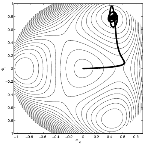
Figure 6.1: Equipotential layers and trajectory of the field $\Phi\equiv(\Phi_{R}+i\Phi_{I})/\sqrt{2}$ in the Kadota and Stewart’s model of Refs. [90, 91]. Figure taken from Ref. [91].

6.5.2 The curvaton model

In the curvaton model [138, 139, 159] (see also Refs. [66, 116, 156] and Subsection 2.4.2) the curvature perturbation $\zeta$ grows, from a negligible value in an initially radiation dominated epoch, due to the oscillations of a weakly coupled light field $\sigma$ (the curvaton) around the minimum of its quadratic potential

$$V_{\sigma}(t,{\bf x})=\frac{1}{2}m_{\sigma}^{2}\sigma^{2}(t,{\bf x})\,,$$ (6.29)

where $m_{\sigma}$ is the curvaton effective mass. Due to the oscillations, the initially negligible curvaton energy density redshifts as

$$\rho_{\sigma}(t,{\bf x})\approx\frac{1}{2}m_{\sigma}^{2}\sigma_{a}^{2}(t,{\bf x})\propto a^{-3}(t,{\bf x})\,,$$ (6.30)

where $\sigma_{a}$ represents the amplitude of the oscillations. Meanwhile the radiation energy density $\rho_{r}$ redshifts as $a^{-4}$. Soon after the curvaton decay, the standard Hot Big-Bang is recovered and $\zeta$ is assumed to be conserved until horizon reentry.

To calculate ${f_{\rm NL}}$ using Eq. (6.20) we first realise that $\sigma_{*}$ (the unperturbed value of $\sigma$ a few Hubble times after horizon exit) is the only relevant quantity since the curvature perturbation produced by the inflaton, and imprinted in the radiation fluid during the reheating process, is supposed to be negligible. Thus, Eq. (6.22) applies. Second, we can redefine $N$ as the number of e-folds from the beginning of the sinusoidal oscillations to the curvaton decay. This is because the number of e-folds from the end of inflation to the beginning of the oscillations is completely unperturbed as the radiation energy density dominates during that time. Thus, $N$ is now a function of three variables

$$N(\rho_{dec},\rho_{osc},\sigma_{*})=\frac{1}{3}\ln\left(\frac{\rho_{\sigma_{\rm osc}}}{\rho_{\sigma_{dec}}}\right)=\frac{1}{3}\ln\left[\frac{\frac{1}{2}m_{\sigma}^{2}[g(\sigma_{*})]^{2}}{\rho_{\sigma_{dec}}}\right]\,,$$ (6.31)

where $g\equiv\sigma_{osc}$ is the amplitude at the beginning of the sinusoidal oscillations as a function of $\sigma_{*}$. Here the curvaton energy density just before the curvaton decay $\rho_{\sigma_{dec}}$ is expressed in terms of the total energy density $\rho_{dec}$ at that time, the total energy density at the beginning of the sinusoidal oscillations $\rho_{osc}$, and $g$ by

$$\rho_{\sigma_{dec}}=\frac{1}{2}m_{\sigma}^{2}[g(\sigma_{*})]^{2}\left(\frac{\rho_{dec}-\rho_{\sigma_{dec}}}{\rho_{osc}}\right)^{3/4}\,.$$ (6.32)

After evaluating $\partial/\partial\sigma_{*}=g^{\prime}\partial/\partial g$, at fixed $\rho_{dec}$ and $\rho_{osc}$, we obtain

$$N_{,\sigma_{\ast}}=\frac{2}{3}r\frac{g^{\prime}}{g}\,,$$ (6.33)

where

$$r\equiv\frac{3\rho_{\sigma_{dec}}}{3\rho_{\sigma_{dec}}+4\rho_{r_{dec}}}\,,$$ (6.34)

being $\rho_{r_{dec}}$ the radiation energy density just before the curvaton decay, giving

$$A_{\zeta}=\frac{H_{\ast}}{2\pi}N_{,\sigma_{\ast}}=\frac{H_{\ast}r}{3\pi}\frac{g^{\prime}}{g}\,,$$ (6.35)

in agreement with first-order cosmological perturbation theory in the sudden decay approximation [138, 139, 159] (see Subsection 2.4.2). Differentiating again we find from Eq. (6.22)

$${f_{\rm NL}}=-\frac{5}{6}\frac{N_{,\sigma_{*}\sigma_{*}}}{N_{,\sigma_{*}}^{2}}=\frac{5}{3}+\frac{5}{6}r-\frac{5}{4r}\left(1+\frac{gg^{\prime\prime}}{g^{\prime 2}}\right)\,,$$ (6.36)

which nicely agrees with the already calculated ${f_{\rm NL}}$ using first- and second-order perturbation theory (see Refs. [17, 126, 131, 138] and Subsection 5.7.4).

6.5.3 Another two-component model

Finally we consider the two-component inflation model of Ref. [67] (see also Refs. [131, 214] and Subsection 5.7.2). For at least some number $N$ of $e$-folds after cosmological scales leave the horizon, the potential in Eq. (5.56) is written as

$$V=V_{h}\left(1+\frac{1}{2}\eta_{\varphi}\frac{\varphi^{2}}{m_{P}^{2}}+\frac{1}{2}\eta_{\vartheta}\frac{\vartheta^{2}}{m_{P}^{2}}\right)\,,$$ (6.37)

with the first term dominating, and $\eta_{\varphi}$ and $\eta_{\vartheta}$ being the slow-roll $\eta$ parameters. The idea is to use Eq. (6.20) to calculate the non-gaussianity after the $N$ e-folds which, barring cancellations, will place a lower limit on the observed non-gaussianity.

The slow-roll equations give the background field values $\varphi_{0}(N)$ and $\vartheta_{0}(N)$ after $N$ e-folds, in terms of those obtaining just after horizon exit

$$\varphi_{0}(N) = \varphi_{0}\exp(-N\eta_{\varphi})\,,$$ (6.38)

$$\vartheta_{0}(N) = \vartheta_{0}\exp(-N\eta_{\vartheta})\,.$$ (6.39)

This gives

$$V_{0}(N,\varphi_{0},\vartheta_{0})=V_{h}\left(1+\frac{1}{2}\eta_{\varphi}\frac{\varphi_{0}^{2}}{m_{P}^{2}}e^{-2N\eta_{\varphi}}+\frac{1}{2}\eta_{\vartheta}\frac{\vartheta_{0}^{2}}{m_{P}^{2}}e^{-2N\eta_{\vartheta}}\right)\,,$$ (6.40)

and allows us to calculate the derivatives of $N$ with respect to $\varphi_{0}$ and $\vartheta_{0}$ at fixed $V$. Focusing on the case $\vartheta_{0}=0$ considered in Ref. [67], we find

$$\zeta=\frac{\delta\varphi}{\eta_{\varphi}\varphi_{0}}-\frac{\eta_{\varphi}}{2}\left(\frac{\delta\varphi}{\eta_{\varphi}\varphi_{0}}\right)^{2}+\frac{\eta_{\vartheta}}{2}e^{2N(\eta_{\varphi}-\eta_{\vartheta})}\left(\frac{\delta\vartheta}{\eta_{\varphi}\varphi_{0}}\right)^{2}\,,$$ (6.41)

in agreement with the second-order perturbation calculation of Ref. [144]. If the observed $\zeta$ has a non-gaussian part $\zeta_{\sigma}$ equal to the last term of Eq. (6.41) and a gaussian part generated mostly after inflation, one can obtain $|{f_{\rm NL}}|>1$ by choosing $\eta_{\varphi}>0.26$, $\eta_{\vartheta}=\eta_{\varphi}/2$, $N=70$, and $\zeta_{\sigma}=10^{-2}\zeta$.

Our calculated expression for the coefficient of $(\delta\vartheta)^{2}$ is in disagreement with the one found in Ref. [214] [c.f. Eq. (5.68)] which uses a set of CPT equations based on those presented in Ref. [3]. After converting the variable used there [131, 217] to our $\zeta$ (see Subsection 5.3.3), these equations give $\dot{\zeta}$ in terms of first-order quantities, but they contain non-local terms involving the inverse Laplacian [133]. Comparison with our non-linear expression in Eq. (6.8) shows that such terms must cancel if correctly evaluated.

6.6 Conclusions

The $\delta N$ formalism is a non-perturbative approach to calculate the curvature perturbation $\zeta$ at all orders, in terms only of background quantities that describe the evolution of a family of unperturbed universes. Such a formalism was originally introduced to calculate the spectrum of $\zeta$ at first order [196, 210, 211] (see also Ref. [110]) in multi-component inflationary models. Now, with the increasing interest in the non-gaussian features of $\zeta$ in both single- and multi-component inflationary models, the formalism has been extended to calculate the curvature perturbation at second order $\zeta_{2}$ and the normalisation ${f_{\rm NL}}$ of the bispectrum [132]. The $\delta N$ formalism relies on the separate universe assumption, which says that on superhorizon scales the Universe behaves locally as if it were unperturbed [12, 127, 140, 197, 222], and on the intrinsic gaussianity of the fields $\phi_{i}$ involved. The quantities $\zeta_{2}$ and ${f_{\rm NL}}$ are easily given in terms of the first and second derivatives of the unperturbed number of e-folds $N$, from an epoch when the fields have assigned values $\phi_{i_{0}}$ to one when the energy density has an assigned value $\rho$, with respect to the unperturbed fields $\phi_{i_{0}}$. The possible intrinsic non-gaussianity of the fields $\phi_{i}$ would lead to an additional contribution to ${f_{\rm NL}}$, highly wavevector dependent [200] but in any case negligible compared to 1 [141]. The $\delta N$ formalism reproduces [132, 200] the well known results in single-component inflation [142], in the curvaton scenario [17, 126, 131, 138], and in the ‘hybrid’ model of Enqvist and V$\ddot{{\rm a}}$ihk$\ddot{{\rm o}}$nen [144]. In addition, the Kadota and Stewart’s modular inflation model [90, 91] has served as an example of the power of this formalism. The $\delta N$ formalism is an interesting alternative to cosmological perturbation theory where, order by order, the relevant expressions to calculate $\zeta_{2}$ and ${f_{\rm NL}}$ tend to be more and more complicated (see for example Refs. [3, 67, 144]). Nevertheless, it is true that the latter is valid on all the scales, while the former is only valid in the superhorizon regime. Fortunately, the subhorizon effects are negligible [141, 200] making the $\delta N$ formalism reliable and completely independent of cosmological perturbation theory.

Chapter 7 Conclusions

Prior to the standard Hot Big-Bang, a period of accelerated expansion seems to have been crucial [79]. Not only does this period solve the classical problems of the Big-Bang cosmological model, namely the horizon, flatness, and unwanted relics problems, but it also amplifies the fluctuations in the light scalar fields $\phi_{i}$ living in the Friedmann-Robertson-Walker spacetime [12, 80, 84, 118, 162, 163, 185, 210]. This inflationary process serves also for the scalar field fluctuations to become classical soon after horizon exit [4, 78, 81, 122, 124], giving birth to the primordial perturbations in the energy density that generate the temperature anisotropies in the cosmic microwave background radiation, and, through gravitational collapse, the large-scale structure observed today. Such primordial perturbations can be defined perturbatively on a homogeneous and isotropic background, but the freedom to choose the perturbed coordinate system makes them gauge dependent. To characterize adequately the primordial perturbations, we introduce the gauge-invariant curvature perturbation $\zeta$ [11] which represents the intrinsic spatial curvature on slices of uniform energy density (or slices with zero flow of energy). While the pressure is a unique function of the energy density, $\zeta$ is conserved at all orders [127, 179], which makes this an ideal quantity. In this thesis we have explored some of the theoretical and statistical aspects of the origin of the large-scale structure, such as the two most known scenarios to generate $\zeta$ (the inflaton and the curvaton scenario), the required inflationary energy scale in those scenarios, and the non-gaussianity associated to $\zeta$.

In general $\zeta$ depends on the perturbations in the scalar fields $\phi_{i}$ during the inflationary period, whose spectra $\mathcal{P}_{\delta\phi_{i}}(k)$ are generically the same for all kinds of quasi exponential expansion either the respective field dominates the energy density or not. The only appreciable difference is in the way the scale dependence is given in terms of the Hubble parameter $H_{\ast}$ a few Hubble times after horizon exit and the mass $m_{\phi_{i}}$ of the respective field. However, the spectrum of $\zeta$, $\mathcal{P}_{\zeta}(k)$, varies significantly among the different possible scenarios for the origin of the large-scale structure, although in all cases it is almost gaussian and scale invariant. We have studied in Chapter 2 two different scenarios for the origin of $\zeta$, the inflaton [5, 112, 117, 130] and the curvaton scenario [138, 139, 159] (see also Refs. [66, 116, 156]), pointing out their different signatures and connecting them with the amplitude of gravitational waves produced in each scenario. Both scenarios have their advantages and drawbacks. For example, the single-component inflaton scenario presents a consistency relation that relates the amplitude of $\mathcal{P}_{\zeta}(k)$ with the amplitude of the gravitational waves spectrum $\mathcal{P}_{T}(k)$ [2, 68, 111, 112, 190]. The possible detection of gravitational waves is consistent with this scenario and would serve as a smoking gun if the consistency relation is satisfied. The drawback is that the generation of $\zeta$ by the inflaton field $\varphi$ (the field which drives inflation) imposes severe constraints on the theoretical model building [49, 160, 161]. In contrast, the curvaton scenario circumvents the latter problem since the generation of $\zeta$ is assigned to a weakly coupled scalar field $\sigma$ (the curvaton) different to the inflaton. The drawbacks are that there is no consistency relation in this case, and that the scenario is inconsistent with a detectable level of gravitational waves [138].

There exists several well motivated inflationary models that locate the inflaton field within a particle physics framework [125, 130]. Most of these models are however unrealistic due to the strong constraints mentioned above. In particular, the generation of adiabatic perturbations is almost inconsistent with the low inflationary energy scale, given by $H_{\ast}$, required to identify the inflaton with one of the many fields present in supersymmetry. The curvaton scenario comes to rescue these models, allowing for a much lower inflationary energy scale. But how low may this energy scale be in the curvaton scenario?. In Chapter 3 we have discussed the lower bound on $H_{\ast}$ in the simplest curvaton setup, showing that it is high enough [126] ($H_{\ast}>10^{7}$ GeV) to fail at rescuing the inflationary models whose potentials are generated by some mechanism of gravity-mediated supersymmetry breaking where $H_{\ast}\sim 10^{3}$ GeV is required. The general conditions to obtain low scale inflation in the curvaton scenario have been given in that chapter [51], in terms of three quantities $\epsilon$, $f$, and $\delta$, that parameterize respectively the evolution of the curvaton field from the time of horizon exit to the beginning of its oscillations, the effective curvaton mass $\tilde{m}_{\sigma}$ at the end of a phase transition with respect to the Hubble parameter at the same time, and the time of the phase transition with respect to the time of horizon exit. In Chapters 3 and 4 we have invoked the ‘heavy curvaton’ picture [126], defined as the setup where $\sigma$ suddenly increases its mass at the end of a phase transition much later than inflation [149]. The mass increment is given by the coupling of $\sigma$ (parameterized by the constant $\lambda$) with another field which acquires a large vacuum expectation value at the end of the same period. Thus, the smallness of the parameters $f$ and $\delta$ are exploited to allow for an inflationary scale consistent with gravity-mediated susy breaking. In the cases presented in these two chapters the phase transition is associated with the end of a second (thermal) inflationary period, which was originally introduced to dilute the abundances of unwanted relics that the first (main) inflationary period is not able to do (for instance the moduli fields) [136, 137]. Thermal inflation is driven by the confinement of a second (flaton) field $\chi$ at the origin of the potential due to the thermal effects from the radiation background left by the inflaton decay [13]. The eventual rolling of $\chi$, towards the minimum of its potential, ends thermal inflation and triggers an increment in the bare mass $m_{\sigma}$ of $\sigma$ through the coupling of the latter with $\chi$. Solving the moduli problem while satisfying adequately all the constraints in the first model discussed in Chapter 3, where the curvaton oscillates for some time before decaying, restricts the parameter space to a region where the two important parameters, $\lambda$ and $m_{\sigma}$, are required to be very small ($10^{-22}\mbox{\raisebox{-3.87495pt}{~{}$\stackrel{{\scriptstyle\mbox{$<$}}}{{\sim}}$~{}}}\lambda\mbox{\raisebox{-3.87495pt}{~{}$\stackrel{{\scriptstyle\mbox{$<$}}}{{\sim}}$~{}}}10^{-10}$ and $m_{\sigma}\mbox{\raisebox{-3.87495pt}{~{}$\stackrel{{\scriptstyle\mbox{$<$}}}{{\sim}}$~{}}}10^{-1}\ {\rm GeV}$) [51]. It is likely then that the curvaton field is a pseudo Nambu-Goldstone boson. In contrast, as discussed in the second model presented in Chapter 4, if the increment in the mass of the curvaton field is so high that the decay rate overtakes the Hubble parameter, leading to the immediate decay of $\sigma$, the parameter space is less constrained, with more natural values for $\lambda$ and $m_{\sigma}$ ($10^{-10}\mbox{\raisebox{-3.87495pt}{~{}$\stackrel{{\scriptstyle\mbox{$<$}}}{{\sim}}$~{}}}\lambda\mbox{\raisebox{-3.87495pt}{~{}$\stackrel{{\scriptstyle\mbox{$<$}}}{{\sim}}$~{}}}10^{-4}$ and $m_{\sigma}\mbox{\raisebox{-3.87495pt}{~{}$\stackrel{{\scriptstyle\mbox{$<$}}}{{\sim}}$~{}}}1\ {\rm GeV}$) [189].

Although $\zeta$ is found to be almost perfectly gaussian in most of the models that give account of its origin, as required by observation, the possibly present small non-gaussianity is being scrutinized by present experiments like the WMAP satellite [223] and will be the focus of future experiments like the PLANCK satellite [171]. The first statistical significant quantity that gives us information about the level of non-gaussianity is the bispectrum, which corresponds to the three-point correlator of $\zeta$ [103]. Its normalisation is given by the parameter ${f_{\rm NL}}$, which has been found to be $|{f_{\rm NL}}|\mbox{\raisebox{-3.87495pt}{~{}$\stackrel{{\scriptstyle\mbox{$<$}}}{{\sim}}$~{}}}10^{2}$ [102] but that will eventually go down to $|{f_{\rm NL}}|\sim 1$ in the forthcoming years unless there is an earlier detection [103]. In view of the difficulty at discriminating between models by means of only the spectral index and/or consistency relations, the detection of non-gaussianity and a precise determination of ${f_{\rm NL}}$ would be useful tools to serve this purpose. For example, in the single-component inflaton scenario the level of non-gaussianity is very small, being $|{f_{\rm NL}}|$ or the order of the slow-roll parameters [142]. In contrast, in the curvaton scenario $|{f_{\rm NL}}|$ could be much higher, being ${f_{\rm NL}}$ negative, or, if $\sigma$ has already dominated the energy density before decaying, the precise value for ${f_{\rm NL}}$ would be ${f_{\rm NL}}=+5/4$ [17, 131, 138]. In Chapters 5 and 6 we have addressed this subject, following a perturbative approach in the former, and a non-perturbative one in the latter. In Chapter 5 we have presented in an unified way the different definitions of the second-order curvature perturbation $\zeta_{2}$ present in the literature [3, 131, 140, 145, 178]. The translation rules to go from one definition to another have been explicitly given, and would help to avoid the possible confusion when confronting different papers and results which use different definitions for $\zeta_{2}$ [131]. We have examined the predictions for ${f_{\rm NL}}$ coming from the single-component inflation model, the multi-component one, and the curvaton scenario, discussing also the respective predictions in preheating and the inhomogeneous reheating scenario. Although multi-component inflation, preheating, and the inhomogeneous reheating scenarios do not predict a definite value or set of values for ${f_{\rm NL}}$, being very dependent on the specific model, the single-component inflaton scenario as well as the curvaton one do give definite predictions for ${f_{\rm NL}}$ [131]. Multi-component slow-roll inflation is studied in Chapter 6 following the non-perturbative $\delta N$ formalism [110, 127, 196, 210, 211], that allows us to calculate $\zeta$ at all orders only by knowing the evolution of a family of unperturbed universes. Immediate applications of this formalism are the calculation of the spectral index [196], and ${f_{\rm NL}}$ [132], in a general multi-component slow-roll inflation model. The formalism relies on the separate universe assumption, which says that the local evolution of the Universe on superhorizon scales is the same as that of an unperturbed universe [12, 127, 140, 197, 222]. The normalisation parameter ${f_{\rm NL}}$ is easily given in terms of first and second derivatives of the number of e-folds, from an initially flat slice to a final uniform energy density slice, with respect to the fields living in the former. The intrinsic non-gaussianity in the fields $\phi_{i}$ relevant for the evolution of the family of universes may be also taken into account, but its contribution, which is highly wavevector dependent [142, 200], is in any case negligible compared to 1 [141]. Comparison of this formalism with cosmological perturbation theory has been made, in the case of the curvaton scenario [132] and the ‘hybrid’ [67] model of Enqvist and V$\ddot{{\rm a}}$ihk$\ddot{{\rm o}}$nen [132, 144, 214]. According to Ref. [144] the results for the latter model following the two approaches agree, and moreover they refute the claim about the possible presence of non-local terms in cosmological perturbation theory [3, 14, 67, 214].

Appendix A ${f_{\rm NL}}$ from the $\delta N$ formalism

In this appendix we derive explicitly the expression in Eq. (6.20) which gives the normalisation ${f_{\rm NL}}$ of the bispectrum of $\zeta$ defined in Eqs. (6.17) and (6.18).

We begin by writing $\zeta$ as given by Eq. (6.12) including the homogeneous term which makes the spatial average of $\zeta$ vanish:

$$\zeta=\sum_{i}N_{,i}\delta\phi_{i}+\frac{1}{2}\sum_{ij}N_{,ij}\delta\phi_{i}\delta\phi_{j}-\frac{1}{2}\sum_{ij}N_{,ij}\langle\delta\phi_{i}\delta\phi_{j}\rangle\,.$$ (A.1)

The corresponding mode function is then written as

$$\zeta_{\bf k}=\sum_{i}N_{,i}\delta_{\bf k}\phi_{i}+\frac{1}{2}\sum_{ij}N_{,ij}\int\frac{d^{3}p}{(2\pi)^{3/2}}\delta_{{\bf k+p}}\phi_{i}\delta_{\bf p}\phi^{\ast}_{j}-\frac{1}{2}(2\pi)^{3/2}\delta^{3}({\bf k})\sum_{ij}N_{,ij}\langle\delta\phi_{i}\delta\phi_{j}\rangle\,.$$ (A.2)

Making use of the above formula, the product of three mode functions $\zeta_{\bf k}$ is therefore

$$\zeta_{{\bf k}_{1}}\zeta_{{\bf k}_{2}}\zeta_{{\bf k}_{3}} = \sum_{ijk}N_{,i}N_{,j}N_{,k}\delta_{{\bf k}_{1}}\phi_{i}\delta_{{\bf k}_{2}}\phi_{j}\delta_{{\bf k}_{3}}\phi_{k}$$

$$+ \frac{1}{2}\sum_{ijkl}N_{,i}N_{,j}N_{,kl}\Big{[}\delta_{{\bf k}_{1}}\phi_{i}\delta_{{\bf k}_{2}}\phi_{j}\int\frac{d^{3}p}{(2\pi)^{3/2}}\delta_{{\bf k}_{3}+{\bf p}}\phi_{k}\delta_{\bf p}\phi_{l}^{\ast}$$

$$+ \delta_{{\bf k}_{1}}\phi_{i}\delta_{{\bf k}_{3}}\phi_{j}\int\frac{d^{3}p}{(2\pi)^{3/2}}\delta_{{\bf k}_{2}+{\bf p}}\phi_{k}\delta_{\bf p}\phi_{l}^{\ast}$$

$$+ \delta_{{\bf k}_{2}}\phi_{i}\delta_{{\bf k}_{3}}\phi_{j}\int\frac{d^{3}p}{(2\pi)^{3/2}}\delta_{{\bf k}_{1}+{\bf p}}\phi_{k}\delta_{\bf p}\phi_{l}^{\ast}\Big{]}$$

$$- \frac{1}{2}(2\pi)^{3/2}\sum_{ijkl}N_{,i}N_{,j}N_{,kl}\Big{[}\delta_{{\bf k}_{1}}\phi_{i}\delta_{{\bf k}_{2}}\phi_{j}\delta^{3}({\bf k}_{3})\langle\delta\phi_{k}\delta\phi_{l}\rangle$$

$$+ \delta_{{\bf k}_{1}}\phi_{i}\delta_{{\bf k}_{3}}\phi_{j}\delta^{3}({\bf k}_{2})\langle\delta\phi_{k}\delta\phi_{l}\rangle$$

$$+ \delta_{{\bf k}_{2}}\phi_{i}\delta_{{\bf k}_{3}}\phi_{j}\delta^{3}({\bf k}_{1})\langle\delta\phi_{k}\delta\phi_{l}\rangle\Big{]}$$

$$+ \frac{1}{4}\sum_{ijklm}N_{,i}N_{,jk}N_{,lm}\Big{[}\int\frac{d^{3}p}{(2\pi)^{3/2}}\frac{d^{3}p^{\prime}}{(2\pi)^{3/2}}\delta_{{\bf k}_{1}}\phi_{i}\delta_{{\bf k}_{2}+{\bf p}}\phi_{j}\delta_{\bf p}\phi_{k}^{\ast}\delta_{{\bf k}_{3}+{\bf p^{\prime}}}\phi_{l}\delta_{\bf p^{\prime}}\phi_{m}^{\ast}$$

$$+ \int\frac{d^{3}p}{(2\pi)^{3/2}}\frac{d^{3}p^{\prime}}{(2\pi)^{3/2}}\delta_{{\bf k}_{2}}\phi_{i}\delta_{{\bf k}_{1}+{\bf p}}\phi_{j}\delta_{\bf p}\phi_{k}^{\ast}\delta_{{\bf k}_{3}+{\bf p^{\prime}}}\phi_{l}\delta_{\bf p^{\prime}}\phi_{m}^{\ast}$$

$$+ \int\frac{d^{3}p}{(2\pi)^{3/2}}\frac{d^{3}p^{\prime}}{(2\pi)^{3/2}}\delta_{{\bf k}_{3}}\phi_{i}\delta_{{\bf k}_{1}+{\bf p}}\phi_{j}\delta_{\bf p}\phi_{k}^{\ast}\delta_{{\bf k}_{2}+{\bf p^{\prime}}}\phi_{l}\delta_{\bf p^{\prime}}\phi_{m}^{\ast}\Big{]}$$

$$- \frac{1}{4}(2\pi)^{3/2}\sum_{ijklm}N_{,i}N_{,jk}N_{,lm}\Big{[}\delta^{3}({\bf k}_{1})\langle\delta\phi_{j}\delta\phi_{k}\rangle\int\frac{d^{3}p}{(2\pi)^{3/2}}\delta_{{\bf k}_{2}}\phi_{i}\delta_{{\bf k}_{3}+{\bf p}}\phi_{l}\delta_{\bf p}\phi_{m}^{\ast}$$

$$+ \delta^{3}({\bf k}_{2})\langle\delta\phi_{j}\delta\phi_{k}\rangle\int\frac{d^{3}p}{(2\pi)^{3/2}}\delta_{{\bf k}_{1}}\phi_{i}\delta_{{\bf k}_{3}+{\bf p}}\phi_{l}\delta_{\bf p}\phi_{m}^{\ast}$$

$$+ \delta^{3}({\bf k}_{3})\langle\delta\phi_{l}\delta\phi_{m}\rangle\int\frac{d^{3}p}{(2\pi)^{3/2}}\delta_{{\bf k}_{1}}\phi_{i}\delta_{{\bf k}_{2}+{\bf p}}\phi_{j}\delta_{\bf p}\phi_{k}^{\ast}$$

$$+ \delta^{3}({\bf k}_{1})\langle\delta\phi_{j}\delta\phi_{k}\rangle\int\frac{d^{3}p}{(2\pi)^{3/2}}\delta_{{\bf k}_{3}}\phi_{i}\delta_{{\bf k}_{2}+{\bf p}}\phi_{l}\delta_{\bf p}\phi_{m}^{\ast}$$

$$+ \delta^{3}({\bf k}_{2})\langle\delta\phi_{j}\delta\phi_{k}\rangle\int\frac{d^{3}p}{(2\pi)^{3/2}}\delta_{{\bf k}_{3}}\phi_{i}\delta_{{\bf k}_{1}+{\bf p}}\phi_{l}\delta_{\bf p}\phi_{m}^{\ast}$$

$$+ \delta^{3}({\bf k}_{3})\langle\delta\phi_{l}\delta\phi_{m}\rangle\int\frac{d^{3}p}{(2\pi)^{3/2}}\delta_{{\bf k}_{2}}\phi_{i}\delta_{{\bf k}_{1}+{\bf p}}\phi_{j}\delta_{\bf p}\phi_{k}^{\ast}\Big{]}$$

$$+ \frac{1}{4}(2\pi)^{3}\sum_{ijklm}N_{,i}N_{,jk}N_{,lm}\Big{[}\delta^{3}({\bf k}_{1})\delta^{3}({\bf k}_{2})\langle\delta\phi_{j}\delta\phi_{k}\rangle\langle\delta\phi_{l}\delta\phi_{m}\rangle\delta_{{\bf k}_{3}}\phi_{i}$$

$$+ \delta^{3}({\bf k}_{1})\delta^{3}({\bf k}_{3})\langle\delta\phi_{j}\delta\phi_{k}\rangle\langle\delta\phi_{l}\delta\phi_{m}\rangle\delta_{{\bf k}_{2}}\phi_{i}$$

$$+ \delta^{3}({\bf k}_{2})\delta^{3}({\bf k}_{3})\langle\delta\phi_{j}\delta\phi_{k}\rangle\langle\delta\phi_{l}\delta\phi_{m}\rangle\delta_{{\bf k}_{1}}\phi_{i}\Big{]}$$

$$+ \frac{1}{8}\sum_{ijklmn}N_{,ij}N_{,kl}N_{,mn}\Big{[}$$

$$\int\frac{d^{3}p}{(2\pi)^{3/2}}\delta_{{\bf k}_{1}+{\bf p}}\phi_{i}\delta_{\bf p}\phi_{j}^{\ast}\int\frac{d^{3}p^{\prime}}{(2\pi)^{3/2}}\delta_{{\bf k}_{2}+{\bf p^{\prime}}}\phi_{k}\delta_{\bf p^{\prime}}\phi_{l}^{\ast}\int\frac{d^{3}p^{\prime\prime}}{(2\pi)^{3/2}}\delta_{{\bf k}_{3}+{\bf p^{\prime\prime}}}\phi_{m}\delta_{\bf p^{\prime\prime}}\phi_{n}^{\ast}\Big{]}$$

$$- \frac{1}{8}(2\pi)^{3/2}\sum_{ijklmn}N_{,ij}N_{,kl}N_{,mn}\Big{[}$$

$$\delta^{3}({\bf k}_{1})\langle\delta\phi_{i}\delta\phi_{j}\rangle\int\frac{d^{3}p}{(2\pi)^{3/2}}\delta_{{\bf k}_{2}+{\bf p}}\phi_{k}\delta_{\bf p}\phi_{l}^{\ast}\int\frac{d^{3}p^{\prime}}{(2\pi)^{3/2}}\delta_{{\bf k}_{3}+{\bf p^{\prime}}}\phi_{m}\delta_{\bf p^{\prime}}\phi_{n}^{\ast}$$

$$+ \delta^{3}({\bf k}_{2})\langle\delta\phi_{k}\delta\phi_{l}\rangle\int\frac{d^{3}p}{(2\pi)^{3/2}}\delta_{{\bf k}_{1}+{\bf p}}\phi_{i}\delta_{\bf p}\phi_{j}^{\ast}\int\frac{d^{3}p^{\prime}}{(2\pi)^{3/2}}\delta_{{\bf k}_{3}+{\bf p^{\prime}}}\phi_{m}\delta_{\bf p^{\prime}}\phi_{n}^{\ast}$$

$$+ \delta^{3}({\bf k}_{3})\langle\delta\phi_{m}\delta\phi_{n}\rangle\int\frac{d^{3}p}{(2\pi)^{3/2}}\delta_{{\bf k}_{1}+{\bf p}}\phi_{i}\delta_{\bf p}\phi_{j}^{\ast}\int\frac{d^{3}p^{\prime}}{(2\pi)^{3/2}}\delta_{{\bf k}_{2}+{\bf p^{\prime}}}\phi_{k}\delta_{\bf p^{\prime}}\phi_{l}^{\ast}\Big{]}$$

$$+ \frac{1}{8}(2\pi)^{3}\sum_{ijklmn}N_{,ij}N_{,kl}N_{,mn}\Big{[}$$

$$\delta^{3}({\bf k}_{1})\delta^{3}({\bf k}_{2})\langle\delta\phi_{i}\delta\phi_{j}\rangle\langle\delta\phi_{k}\delta\phi_{l}\rangle\int\frac{d^{3}p}{(2\pi)^{3/2}}\delta_{{\bf k}_{3}+{\bf p}}\phi_{m}\delta_{\bf p}\phi_{n}^{\ast}$$

$$+ \delta^{3}({\bf k}_{1})\delta^{3}({\bf k}_{3})\langle\delta\phi_{i}\delta\phi_{j}\rangle\langle\delta\phi_{m}\delta\phi_{n}\rangle\int\frac{d^{3}p}{(2\pi)^{3/2}}\delta_{{\bf k}_{2}+{\bf p}}\phi_{k}\delta_{\bf p}\phi_{l}^{\ast}$$

$$+ \delta^{3}({\bf k}_{2})\delta^{3}({\bf k}_{3})\langle\delta\phi_{k}\delta\phi_{l}\rangle\langle\delta\phi_{m}\delta\phi_{n}\rangle\int\frac{d^{3}p}{(2\pi)^{3/2}}\delta_{{\bf k}_{1}+{\bf p}}\phi_{i}\delta_{\bf p}\phi_{j}^{\ast}\Big{]}$$

$$- \frac{1}{8}(2\pi)^{9/2}\sum_{ijklmn}N_{,ij}N_{,kl}N_{,mn}\delta^{3}({\bf k}_{1})\delta^{3}({\bf k}_{2})\delta^{3}({\bf k}_{3})\langle\delta\phi_{i}\delta\phi_{j}\rangle\langle\delta\phi_{k}\delta\phi_{l}\rangle\langle\delta\phi_{m}\delta\phi_{n}\rangle\,.$$

The next step is to take the average of the latter expression. In doing so, we make use of the following decompositions [14]:

$$\langle\delta_{{\bf k}_{1}}\phi_{i}\delta_{{\bf k}_{2}}\phi_{j}\delta_{{\bf k}_{3}}\phi_{k}\delta_{{\bf k}_{4}}\phi_{l}\rangle=$$

$$\langle\delta_{{\bf k}_{1}}\phi_{i}\delta_{{\bf k}_{2}}\phi_{j}\rangle\langle\delta_{{\bf k}_{3}}\phi_{k}\delta_{{\bf k}_{4}}\phi_{l}\rangle+\langle\delta_{{\bf k}_{1}}\phi_{i}\delta_{{\bf k}_{3}}\phi_{k}\rangle\langle\delta_{{\bf k}_{2}}\phi_{j}\delta_{{\bf k}_{4}}\phi_{l}\rangle+\langle\delta_{{\bf k}_{1}}\phi_{i}\delta_{{\bf k}_{4}}\phi_{l}\rangle\langle\delta_{{\bf k}_{2}}\phi_{j}\delta_{{\bf k}_{3}}\phi_{k}\rangle\,,$$

(A.4)

$$\langle\delta_{{\bf k}_{1}}\phi_{i}\delta_{{\bf k}_{2}}\phi_{j}\delta_{{\bf k}_{3}}\phi_{k}\delta_{{\bf k}_{4}}\phi_{l}\delta_{{\bf k}_{5}}\phi_{m}\delta_{{\bf k}_{6}}\phi_{n}\rangle=$$

$$\langle\delta_{{\bf k}_{1}}\phi_{i}\delta_{{\bf k}_{2}}\phi_{j}\rangle\langle\delta_{{\bf k}_{3}}\phi_{k}\delta_{{\bf k}_{4}}\phi_{l}\rangle\langle\delta_{{\bf k}_{5}}\phi_{m}\delta_{{\bf k}_{6}}\phi_{n}\rangle+\langle\delta_{{\bf k}_{1}}\phi_{i}\delta_{{\bf k}_{2}}\phi_{j}\rangle\langle\delta_{{\bf k}_{3}}\phi_{k}\delta_{{\bf k}_{5}}\phi_{m}\rangle\langle\delta_{{\bf k}_{4}}\phi_{l}\delta_{{\bf k}_{6}}\phi_{n}\rangle$$

$$+ \langle\delta_{{\bf k}_{1}}\phi_{i}\delta_{{\bf k}_{2}}\phi_{j}\rangle\langle\delta_{{\bf k}_{3}}\phi_{k}\delta_{{\bf k}_{6}}\phi_{n}\rangle\langle\delta_{{\bf k}_{4}}\phi_{l}\delta_{{\bf k}_{5}}\phi_{m}\rangle+\langle\delta_{{\bf k}_{1}}\phi_{i}\delta_{{\bf k}_{3}}\phi_{k}\rangle\langle\delta_{{\bf k}_{2}}\phi_{j}\delta_{{\bf k}_{4}}\phi_{l}\rangle\langle\delta_{{\bf k}_{5}}\phi_{m}\delta_{{\bf k}_{6}}\phi_{n}\rangle$$

$$+ \langle\delta_{{\bf k}_{1}}\phi_{i}\delta_{{\bf k}_{3}}\phi_{k}\rangle\langle\delta_{{\bf k}_{2}}\phi_{j}\delta_{{\bf k}_{5}}\phi_{m}\rangle\langle\delta_{{\bf k}_{4}}\phi_{l}\delta_{{\bf k}_{6}}\phi_{n}\rangle+\langle\delta_{{\bf k}_{1}}\phi_{i}\delta_{{\bf k}_{3}}\phi_{k}\rangle\langle\delta_{{\bf k}_{2}}\phi_{j}\delta_{{\bf k}_{6}}\phi_{n}\rangle\langle\delta_{{\bf k}_{4}}\phi_{l}\delta_{{\bf k}_{5}}\phi_{m}\rangle$$

$$+ \langle\delta_{{\bf k}_{1}}\phi_{i}\delta_{{\bf k}_{4}}\phi_{l}\rangle\langle\delta_{{\bf k}_{2}}\phi_{j}\delta_{{\bf k}_{3}}\phi_{k}\rangle\langle\delta_{{\bf k}_{5}}\phi_{m}\delta_{{\bf k}_{6}}\phi_{n}\rangle+\langle\delta_{{\bf k}_{1}}\phi_{i}\delta_{{\bf k}_{4}}\phi_{l}\rangle\langle\delta_{{\bf k}_{2}}\phi_{j}\delta_{{\bf k}_{5}}\phi_{m}\rangle\langle\delta_{{\bf k}_{3}}\phi_{k}\delta_{{\bf k}_{6}}\phi_{n}\rangle$$

$$+ \langle\delta_{{\bf k}_{1}}\phi_{i}\delta_{{\bf k}_{4}}\phi_{l}\rangle\langle\delta_{{\bf k}_{2}}\phi_{j}\delta_{{\bf k}_{6}}\phi_{n}\rangle\langle\delta_{{\bf k}_{3}}\phi_{k}\delta_{{\bf k}_{5}}\phi_{m}\rangle+\langle\delta_{{\bf k}_{1}}\phi_{i}\delta_{{\bf k}_{5}}\phi_{m}\rangle\langle\delta_{{\bf k}_{2}}\phi_{j}\delta_{{\bf k}_{3}}\phi_{k}\rangle\langle\delta_{{\bf k}_{4}}\phi_{l}\delta_{{\bf k}_{6}}\phi_{n}\rangle$$

$$+ \langle\delta_{{\bf k}_{1}}\phi_{i}\delta_{{\bf k}_{5}}\phi_{m}\rangle\langle\delta_{{\bf k}_{2}}\phi_{j}\delta_{{\bf k}_{4}}\phi_{l}\rangle\langle\delta_{{\bf k}_{3}}\phi_{k}\delta_{{\bf k}_{6}}\phi_{n}\rangle+\langle\delta_{{\bf k}_{1}}\phi_{i}\delta_{{\bf k}_{5}}\phi_{m}\rangle\langle\delta_{{\bf k}_{2}}\phi_{j}\delta_{{\bf k}_{6}}\phi_{n}\rangle\langle\delta_{{\bf k}_{3}}\phi_{k}\delta_{{\bf k}_{4}}\phi_{l}\rangle$$

$$+ \langle\delta_{{\bf k}_{1}}\phi_{i}\delta_{{\bf k}_{6}}\phi_{n}\rangle\langle\delta_{{\bf k}_{2}}\phi_{j}\delta_{{\bf k}_{3}}\phi_{k}\rangle\langle\delta_{{\bf k}_{4}}\phi_{l}\delta_{{\bf k}_{5}}\phi_{m}\rangle+\langle\delta_{{\bf k}_{1}}\phi_{i}\delta_{{\bf k}_{6}}\phi_{n}\rangle\langle\delta_{{\bf k}_{2}}\phi_{j}\delta_{{\bf k}_{4}}\phi_{l}\rangle\langle\delta_{{\bf k}_{3}}\phi_{k}\delta_{{\bf k}_{5}}\phi_{m}\rangle$$

$$+ \langle\delta_{{\bf k}_{1}}\phi_{i}\delta_{{\bf k}_{6}}\phi_{n}\rangle\langle\delta_{{\bf k}_{2}}\phi_{j}\delta_{{\bf k}_{5}}\phi_{m}\rangle\langle\delta_{{\bf k}_{3}}\phi_{k}\delta_{{\bf k}_{4}}\phi_{l}\rangle\,,$$

where we have neglected connected $n$-point correlators with $n>3$, which nobody has calculated yet but that are presumably very small [200], and products of $n$-point correlators with $m$-point correlators, where $n\geq 3$ and $m\geq 2$, which we believe give a much smaller contribution than that coming from the three-point correlator [135].

From Eqs. (LABEL:barethreepoint), (A.4), and (LABEL:decom6), and after doing some algebra, we obtain the three point correlator function of the $\zeta_{\bf k}$ mode functions:

$$\langle\zeta_{{\bf k}_{1}}\zeta_{{\bf k}_{2}}\zeta_{{\bf k}_{3}}\rangle=\sum_{ijk}N_{,i}N_{,j}N_{,k}\langle\delta_{{\bf k}_{1}}\phi_{i}\delta_{{\bf k}_{2}}\phi_{j}\delta_{{\bf k}_{3}}\phi_{k}\rangle$$

$$+\sum_{ij}N_{,i}N_{,j}N_{,ij}(2\pi)^{-3/2}\delta^{3}({\bf k}_{1}+{\bf k}_{2}+{\bf k}_{3})\left(\frac{H_{\ast}}{2\pi}\right)^{4}\left[\frac{4\pi^{4}}{k_{1}^{3}k_{2}^{3}}+{\rm cyclic}\ {\rm permutations}\right]$$

$$+\frac{1}{2}\sum_{ijk}N_{,ij}N_{,jk}N_{,ki}(2\pi)^{-3/2}\delta^{3}({\bf k}_{1}+{\bf k}_{2}+{\bf k}_{3})\left(\frac{H_{\ast}}{2\pi}\right)^{6}\times$$

$$\times\int d^{3}p\left[\frac{1}{|{\bf k}_{1}+{\bf p}|^{3}p^{3}|{\bf k}_{3}-{\bf p}|^{3}}+\frac{1}{|{\bf k}_{1}+{\bf p}|^{3}p^{3}|{\bf k}_{2}-{\bf p}|^{3}}\right]\,.$$ (A.6)

The integrals in the last line of the previous expression are calculated following the arguments presented in Ref. [32], giving as a result

$$\int d^{3}p\left[\frac{1}{|{\bf k}_{1}+{\bf p}|^{3}p^{3}|{\bf k}_{3}-{\bf p}|^{3}}+\frac{1}{|{\bf k}_{1}+{\bf p}|^{3}p^{3}|{\bf k}_{2}-{\bf p}|^{3}}\right]=8\pi\ln(kL)\left[\frac{1}{k_{1}^{3}k_{2}^{3}}+{\rm cyclic}\right]\,,$$ (A.7)

where $k^{-1}$ represents a typical scale under consideration and $L$ is the size of the region within which the stochastic properties are specified. That is why $\ln(kL)$ can be taken of order 1.

Finally, making use of the ${f_{\rm NL}}$ definition in Eqs. (6.17) and (6.18):

$${\langle{\zeta_{{\bf k}_{1}}\zeta_{{\bf k}_{2}}\zeta_{{\bf k}_{3}}}\rangle}={(2\pi)}^{-3/2}\delta^{3}({\bf k}_{1}+{\bf k}_{2}+{\bf k}_{3})\left[-\frac{6}{5}{f_{\rm NL}}(k_{1},k_{2},k_{3})[P_{\zeta}(k_{1})P_{\zeta}(k_{2})+{\rm cyclic}]\right]\,,$$ (A.8)

the results found in Eqs. (A.6) and (A.7), and the expression in Eq. (6.16) for the amplitude of the spectrum of $\zeta$ in terms of the first derivatives of $N$:

$$A_{\zeta}^{2}=\left(\frac{H_{\ast}}{2\pi}\right)^{2}\sum_{i}N_{,i}^{2}\,,$$ (A.9)

we arrive to the desired expression

$$-\frac{3}{5}{f_{\rm NL}}=\frac{\sum_{ij}{N_{,i}}{N_{,j}}{N_{,ij}}}{2\left[\sum_{i}{N_{,i}}^{2}\right]^{2}}+\ln(kL)\frac{A_{\zeta}^{2}}{2}\frac{\sum_{ijk}{N_{,ij}}N_{,jk}N_{,ki}}{\left[\sum_{i}{N_{,i}}^{2}\right]^{3}}\,,$$ (A.10)

with an additional contribution

$$\Delta{f_{\rm NL}}=\frac{\sum_{ijk}{N_{,i}}{N_{,j}}N_{,k}f_{ijk}(k_{1},k_{2},k_{3})}{\left(\sum_{i}{N_{,i}}^{2}\right)^{3/2}}|A_{\zeta}^{-1}|\,.$$ (A.11)

The latter expression comes from the first line in Eq. (A.6) containing the three-point correlator $\langle\delta_{{\bf k}_{1}}\phi_{i}\delta_{{\bf k}_{2}}\phi_{j}\delta_{{\bf k}_{3}}\phi_{k}\rangle$. This three-point correlator is normalised in such a way that the bispectra $B_{ijk}$ of the dimensionless perturbations $(2\pi/H_{\ast})\delta\phi_{i}$ is written in the same way as in Eqs. (6.17) and (6.18) with ${f_{\rm NL}}(k_{1},k_{2},k_{3})$ being replaced by $f_{ijk}(k_{1},k_{2},k_{3})$.

Bibliography

- [1] Anglo-Australian Observatory’s 2-degree Field Galaxy Redshift Survey homepage: http://www.mso.anu.edu.au/2dFGRS/.
- [2] L. F. Abbott and M. B. Wise, Constraints on generalized inflationary cosmologies, Nucl. Phys. B 244, 541 (1984).
- [3] V. Acquaviva, N. Bartolo, S. Matarrese, and A. Riotto, Gauge-invariant second-order perturbations and non-Gaussianity from inflation, Nucl. Phys. B 667, 119 (2003).
- [4] A. Albrecht, P. Ferreira, M. Joyce, and T. Prokopec, Inflation and squeezed quantum states, Phys. Rev. D 50, 4807 (1994).
- [5] A. Albrecht and P. J. Steinhardt, Cosmology for grand unified theories with radiatively induced symmetry breaking, Phys. Rev. Lett. 48, 1220 (1982).
- [6] R. A. Alpher, H. A. Bethe, and G. Gamow, The origin of chemical elements, Phys. Rev. 73, 803 (1948).
- [7] R. A. Alpher, J. W. Follin, and R. C. Herman, Physical conditions in the initial stages of the expanding Universe, Phys. Rev. 92, 1347 (1953).
- [8] S. Antusch, M. Bastero-Gil, S. F. King, and Q. Shafi, Sneutrino hybrid inflation in supergravity, Phys. Rev. D 71, 083519 (2005).
- [9] N. Arkani-Hamed, P. Creminelli, S. Mukohyama, and M. Zaldarriaga, Ghost inflation, JCAP 0404, 001 (2004).
- [10] T. Banks, D. B. Kaplan, and A. E. Nelson, Cosmological implications of dynamical supersymmetry breaking, Phys. Rev. D 49, 779 (1994).
- [11] J. M. Bardeen, Gauge-invariant cosmological perturbations, Phys. Rev. D 22, 1882 (1980).
- [12] J. M. Bardeen, P. J. Steinhardt, and M. S. Turner, Spontaneous creation of almost scale-free density perturbations in an inflationary Universe, Phys. Rev. D 28, 679 (1983).
- [13] T. Barreiro, E. J. Copeland, D. H. Lyth, and T. Prokopec, Some aspects of thermal inflation: the finite temperature potential and topological defects, Phys. Rev. D 54, 1379 (1996).
- [14] N. Bartolo, E. Komatsu, S. Matarrese, and A. Riotto, Non-Gaussianity from inflation: theory and observations, Phys. Rep. 402, 103 (2004).
- [15] N. Bartolo, S. Matarrese, and A. Riotto, Non-Gaussianity from inflation, Phys. Rev. D 65, 103505 (2002).
- [16] N. Bartolo, S. Matarrese, and A. Riotto, Enhancement of non-gaussianity after inflation, JHEP 0404, 006 (2004).
- [17] N. Bartolo, S. Matarrese, and A. Riotto, Non-Gaussianity in the curvaton scenario, Phys. Rev. D 69, 043503 (2004).
- [18] N. Bartolo, S. Matarrese, and A. Riotto, Evolution of second-order cosmological perturbations and non-Gaussianity, JCAP 0401, 003 (2004).
- [19] N. Bartolo, S. Matarrese, and A. Riotto, Gauge-invariant temperature anisotropies and primordial non-Gaussianity, Phys. Rev. Lett. 93, 231301 (2004).
- [20] N. Bartolo, S. Matarrese, and A. Riotto, Non-Gaussianity of large-scale cosmic microwave background anisotropies beyond perturbation theory, JCAP 0508, 010 (2005).
- [21] B. A. Bassett, D. I. Kaiser, and R. Maartens, General relativistic preheating after inflation, Phys. Lett. B 455, 84 (1999).
- [22] B. A. Bassett, F. Tamburini, D. I. Kaiser, and R. Maartens, Metric preheating and limitations of linearized gravity, Nucl. Phys. B 561, 188 (1999).
- [23] B. A. Bassett, S. Tsujikawa, and D. Wands, Inflation dynamics and reheating, astro-ph/0507632.
- [24] M. Bastero-Gil, V. Di Clemente, and S. F. King, A supersymmetric standard model of inflation with extra dimensions, Phys. Rev. D 67, 083504 (2003).
- [25] M. Bastero-Gil, V. Di Clemente, and S. F. King, Large-scale structure from the Higgs fields of the Supersymmetric Standard Model, Phys. Rev. D 67, 103516 (2003).
- [26] C. L. Bennett et. al., First year Wilkinson Microwave Anisotropy Probe (WMAP) observations: preliminary maps and basic results, Astrophys. J. Suppl. Ser. 148, 1 (2003).
- [27] M. Berkooz, D. J. H. Chung, and T. Volansky, Constraining modular inflation in the MSSM from giant Q-ball formation, hep-ph/0507218.
- [28] F. Bernardeau and J. P. Uzan, Non-Gaussianity in multifield inflation, Phys. Rev. D 66, 103506 (2002).
- [29] F. Bernardeau and J. P. Uzan, Inflationary models inducing non-Gaussian metric fluctuations, Phys. Rev. D 67, 121301(R) (2003).
- [30] N. D. Birrell and P. C. W. Davies, Quantum fields in curved space, Cambridge University Press, Cambridge UK, 1982.
- [31] L. Boubekeur and D. H. Lyth, Hilltop inflation, JCAP 0507, 010 (2005).
- [32] L. Boubekeur and D. H. Lyth, Detecting a small perturbation through its non-Gaussianity, astro-ph/0504046.
- [33] B. Brahmachari and R. N. Mohapatra, Low intermediate scale SUSY SO(10) and its implications, Phys. Lett. B 357, 566 (1995).
- [34] B. Brahmachari and R. N. Mohapatra, A low and its consequences for unified model building, Int. J. Mod. Phys. A 11, 1699 (1996).
- [35] R. H. Brandenberger, Quantum fluctuations as the source of classical gravitational perturbations in inflationary Universe models, Nucl. Phys. B 245, 328 (1984).
- [36] M. Bruni, S. Matarrese, S. Mollerach, and S. Sonego, Perturbations of spacetime: gauge transformations and gauge invariance at second order and beyond, Class. Quantum Grav. 14, 2585 (1997).
- [37] T. S. Bunch and P. C. W. Davies, Quantum field theory in de Sitter space: renormalization by point splitting, Proc. R. Soc. Lond. A 360, 117 (1978).
- [38] G. Calcagni, Non-Gaussianity in braneworld and tachyon inflation, astro-ph/0411773.
- [39] B. de Carlos, J. A. Casas, F. Quevedo, and E. Roulet, Model independent properties and cosmological implications of the dilaton and moduli sectors of 4D strings, Phys. Lett. B 318, 447 (1993).
- [40] E. J. Chun, K. Dimopoulos, and D. H. Lyth, Curvaton and QCD axion in supersymmetric theories, Phys. Rev. D 70, 103510 (2004).
- [41] M. Colless, The 2dF Galaxy Redshift Survey: spectra and redshifts, Mon. Not. R. Astron. Soc. 328, 1039 (2001).
- [42] G. D. Coughlan, W. Fischler, E. W. Kolb, S. Raby, and G. G. Ross, Cosmological problems for the polonyi potential, Phys. Lett. B 131, 59 (1983).
- [43] P. Creminelli, On non-Gaussianities in single-field inflation, JCAP 0310, 003 (2003).
- [44] P. Creminelli and M. Zaldarriaga, A single-field consistency relation for the three-point function, JCAP 0410, 006 (2004).
- [45] P. Creminelli and M. Zaldarriaga, CMB 3-point functions generated by non-linearities at recombination, Phys. Rev. D 70, 083532 (2004).
- [46] R. H. Dicke, P. J. E. Peebles, P. G. Roll, and D. T. Wilkinson, Cosmic black-body radiation, Astrophys. J. 142, 414 (1965).
- [47] K. Dimopoulos, G. Lazarides, D. H. Lyth, and R. Ruiz de Austri, Curvaton dynamics, Phys. Rev. D 68, 123515 (2003).
- [48] K. Dimopoulos, G. Lazarides, D. H. Lyth, and R. Ruiz de Austri, The Peccei-Quinn field as curvaton, JHEP 0305, 057 (2003).
- [49] K. Dimopoulos and D. H. Lyth, Models of inflation liberated by the curvaton hypothesis, Phys. Rev. D 69, 123509 (2004).
- [50] K. Dimopoulos, D. H. Lyth, A. Notari, and A. Riotto, The curvaton as a pseudo-Nambu-Goldstone boson, JHEP 0307, 053 (2003).
- [51] K. Dimopoulos, D. H. Lyth, and Y. Rodríguez, Low scale inflation and the curvaton mechanism, JHEP 0502, 055 (2005).
- [52] M. Dine and A. Riotto, An inflaton candidate in gauge mediated supersymmetry breaking, Phys. Rev. Lett. 79, 2632 (1997).
- [53] G. Dvali, A. Gruzinov, and M. Zaldarriaga, New mechanism for generating density perturbations from inflation, Phys. Rev. D 69, 023505 (2004).
- [54] G. Dvali, A. Gruzinov, and M. Zaldarriaga, Cosmological perturbations from inhomogeneous reheating, freeze-out, and mass domination, Phys. Rev. D 69, 083505 (2004).
- [55] J. R. Ellis, G. B. Gelmini, J. L. López, D. V. Nanopoulos, and S. Sarkar, Astrophysical constraints on massive unstable neutral relic particles, Nucl. Phys. B 373, 399 (1992).
- [56] J. R. Ellis, A. D. Linde, and D. V. Nanopoulos, Inflation can save the gravitino, Phys. Lett. B 118, 59 (1982).
- [57] J. R. Ellis, D. V. Nanopoulos, and M. Quirós, On the axion, dilaton, polonyi, gravitino and shadow matter problems in supergravity and superstring models, Phys. Lett. B 174, 176 (1986).
- [58] K. Enqvist, Curvatons in the Minimally Supersymmetric Standard Model, Mod. Phys. Lett. A 19, 1421 (2004).
- [59] K. Enqvist, A. Jokinen, S. Kasuya, and A. Mazumdar, MSSM flat direction as a curvaton, Phys. Rev. D 68, 103507 (2003).
- [60] K. Enqvist, A. Jokinen, A. Mazumdar, T. Multamki, and A. Vihknen, Non-Gaussianity from preheating, Phys. Rev. Lett. 94, 161301 (2005).
- [61] K. Enqvist, A. Jokinen, A. Mazumdar, T. Multamki, and A. Vihknen, Non-Gaussianity from instant and tachyonic preheating, JCAP 0503, 010 (2005).
- [62] K. Enqvist, A. Jokinen, A. Mazumdar, T. Multamki, and A. Vihknen, Cosmological constraints on string scale and coupling arising from tachyonic instability, JHEP 0508, 084 (2005).
- [63] K. Enqvist, S. Kasuya, and A. Mazumdar, Adiabatic density perturbations and matter generation from the Minimal Supersymmetric Standard Model, Phys. Rev. Lett. 90, 091302 (2003).
- [64] K. Enqvist and A. Mazumdar, Cosmological consequences of MSSM flat directions, Phys. Rep. 380, 99 (2003).
- [65] K. Enqvist, A. Mazumdar, and M. Postma, Challenges in generating density perturbations from a fluctuating inflaton coupling, Phys. Rev. D 67, 121303 (2003).
- [66] K. Enqvist and M. S. Sloth, Adiabatic CMB perturbations in pre-Big Bang string cosmology, Nucl. Phys. B 626, 395 (2002).
- [67] K. Enqvist and A. Vihknen, Non-Gaussian perturbations in hybrid inflation, JCAP 0409, 006 (2004).
- [68] R. Fabbri and M. D. Pollock, The effect of primordially produced gravitons upon the anisotropy of the cosmological microwave background radiation, Phys. Lett. B 125, 445 (1983).
- [69] T. Falk, R. Rangarajan, and M. Srednicki, The angular dependence of the three-point correlation function of the cosmic microwave background radiation as predicted by inflationary cosmologies, Astrophys. J. 403, L1 (1993).
- [70] F. Ferrer, S. Rsnen, and J. Vliviita, Correlated isocurvature perturbations from mixed inflaton-curvaton decay, JCAP 0410, 010 (2004).
- [71] J. Foster and J. D. Nightingale, A short course in general relativity, Longman, New York USA, 1979.
- [72] A. Friedmann, ber die Krmmung des Raumes, Z. Phys. 10, 377 (1922) [On the curvature of space, Gen. Rel. Grav. 31, 1991 (1999)].
- [73] G. Gamow, Expanding Universe and the origin of elements, Phys. Rev. 70, 572 (1946).
- [74] A. Gangui, F. Lucchin, S. Matarrese, and S. Mollerach, The three-point correlation function of the cosmic microwave background in inflationary models, Astrophys. J. 430, 447 (1994).
- [75] J. García-Bellido, The evolution of the Universe, hep-ph/0303153.
- [76] T. Gherghetta, C. F. Kolda, and S. P. Martin, Flat directions in the scalar potential of the Supersymmetric Standard Model, Nucl. Phys. B 468, 37 (1996).
- [77] C. Gordon, D. Wands, B. A. Bassett, and R. Maartens, Adiabatic and entropy perturbations from inflation, Phys. Rev. D 63, 023506 (2000).
- [78] L. P. Grishchuk, Cosmological perturbations of quantum mechanical origin and anisotropy of the microwave background, Phys. Rev. Lett. 70, 2371 (1993).
- [79] A. H. Guth, The inflationary Universe: a possible solution to the horizon and flatness problems, Phys. Rev. D 23, 347 (1981).
- [80] A. H. Guth and S.-Y. Pi, Fluctuations in the new inflationary Universe, Phys. Rev. Lett. 49, 1110 (1982).
- [81] A. H. Guth and S.-Y. Pi, The quantum mechanics of the scalar field in the new inflationary Universe, Phys. Rev. D 32, 1899 (1985).
- [82] K. Hamaguchi, M. Kawasaki, T. Moroi, and F. Takahashi, Curvatons in supersymmetric models, Phys. Rev. D 69, 063504 (2004).
- [83] T. Hattori and K. Yamamoto, Non-Gaussianity in multi-field stochastic inflation with the scaling approximation, JCAP 0507, 005 (2005).
- [84] S. W. Hawking, The development of irregularities in a single bubble inflationary Universe, Phys. Lett. B 115, 295 (1982).
- [85] C. M. Hirata and U. Seljak, Reconstruction of lensing from the cosmic microwave background polarization, Phys. Rev. D 68, 083002 (2003).
- [86] R. Hofmann, The curvaton as a Bose-Einstein condensate of chiral pseudo Nambu-Goldstone bosons, hep-ph/0208267.
- [87] F. Hoyle and R. J. Tayler, The mystery of the cosmic helium abundance, Nature 203, 1108 (1964).
- [88] W. Hu, Angular trispectrum of the CMB, Phys. Rev. D 64, 083005 (2001).
- [89] J.-C. Hwang, Gravitational wave spectra from pole-like inflations based on generalized gravity theories, Class. Quantum Grav. 15, 1401 (1998).
- [90] K. Kadota and E. D. Stewart, Successful modular cosmology, JHEP 0307, 013 (2003).
- [91] K. Kadota and E. D. Stewart, Inflation on moduli space and cosmic perturbations, JHEP 0312, 008 (2003).
- [92] S. Kasuya, M. Kawasaki, and F. Takahashi, MSSM curvaton in the gauge-mediated SUSY breaking, Phys. Lett. B 578, 259 (2004).
- [93] S. Kasuya, T. Moroi, and F. Takahashi, Can MSSM particle be the inflaton?, Phys. Lett. B 593, 33 (2004).
- [94] M. Kesden, A. Cooray, and M. Kamionkowski, Separation of gravitational-wave and cosmic-shear contributions to cosmic microwave background polarization, Phys. Rev. Lett. 89, 011304 (2002).
- [95] L. Knox and Y. Song, A limit on the detectability of the energy scale of inflation, Phys. Rev. Lett. 89, 011303 (2002).
- [96] H. Kodama and M. Sasaki, Cosmological perturbation theory, Prog. Theor. Phys. Suppl. 78, 1 (1984).
- [97] L. Kofman, Probing string theory with modulated cosmological fluctuations, astro-ph/0303614.
- [98] L. Kofman, A. Linde and A. A. Starobinsky, Reheating after inflation, Phys. Rev. Lett. 73, 3195 (1994).
- [99] L. Kofman, A. Linde and A. A. Starobinsky, Towards the theory of reheating after inflation, Phys. Rev. D 56, 3258 (1997).
- [100] E. W. Kolb, A. Riotto, and A. Vallinotto, Curvature perturbations from broken symmetries, Phys. Rev. D 71, 043513 (2005).
- [101] E. W. Kolb and M. S. Turner, The early Universe, Addison-Wesley, Redwood City USA, 1990.
- [102] E. Komatsu et al., First-year Wilkinson Microwave Anisotropy Probe (WMAP) observations: tests of gaussianity, Astrophys. J. Suppl. Ser. 148, 119 (2003).
- [103] E. Komatsu and D. N. Spergel, Acoustic signatures in the primary microwave background bispectrum, Phys. Rev. D 63, 063002 (2001).
- [104] O. Lahav et. al., The 2dF Galaxy Redshift Survey: the amplitude of fluctuations in the 2dFGRS and the CMB, and implications for galaxy biasing, Mon. Not. R. Astron. Soc. 333, 961 (2002).
- [105] D. Langlois and F. Vernizzi, Mixed inflaton and curvaton perturbations, Phys. Rev. D 70, 063522 (2004).
- [106] D. Langlois and F. Vernizzi, Evolution of non-linear cosmological perturbations, Phys. Rev. Lett. 95, 091303 (2005).
- [107] D. Langlois and F. Vernizzi, Conserved non-linear quantities in cosmology, astro-ph/0509078.
- [108] G. Lazarides, C. Panagiotakopoulos, and Q. Shafi, Baryogenesis and the gravitino problem in superstring models, Phys. Rev. Lett. 56, 557 (1986).
- [109] D.-G. Lee and R. N. Mohapatra, Intermediate scales in SUSY SO(10), unification, and hot dark matter neutrinos, Phys. Rev. D 52, 4125 (1995).
- [110] H.-C. Lee, M. Sasaki, E. D. Stewart, T. Tanaka, and S. Yokoyama, A new formalism for multi-component inflation, astro-ph/0506262.
- [111] A. R. Liddle and D. H. Lyth, COBE, gravitational waves, inflation and extended inflation, Phys. Lett. B 291, 391 (1992).
- [112] A. R. Liddle and D. H. Lyth, Cosmological inflation and large-scale structure, Cambridge University Press, Cambridge UK, 2000.
- [113] A. R. Liddle, D. H. Lyth, K. A. Malik, and D. Wands, Superhorizon perturbations and preheating, Phys. Rev. D 61, 103509 (2000).
- [114] E. M. Lifshitz, On the gravitational stability of the expanding Universe, J. Phys. (USSR) 10, 116 (1946).
- [115] A. Linde, Fast-roll inflation, JHEP 0111, 052 (2001).
- [116] A. Linde and V. Mukhanov, Non-Gaussian isocurvature perturbations from inflation, Phys. Rev. D 56, R535 (1997).
- [117] A. D. Linde, A new inflationary Universe scenario: a possible solution of the horizon, flatness, homogeneity, isotropy and primordial monopole problems, Phys. Lett. B 108, 389 (1982).
- [118] A. D. Linde, Scalar field fluctuations in expanding Universe and the new inflationary Universe scenario, Phys. Lett. B 116, 335 (1982).
- [119] A. D. Linde, Eternal extended inflation and graceful exit from old inflation without Jordan-Brans-Dicke, Phys. Lett. B 249, 18 (1990).
- [120] A. D. Linde, Axions in inflationary cosmology, Phys. Lett. B 259, 38 (1991).
- [121] A. D. Linde, Hybrid inflation, Phys. Rev. D 49, 748 (1994).
- [122] F. Lombardo and D. López Nacir, Decoherence during inflation: the generation of classical inhomogeneities, Phys. Rev. D 72, 063506 (2005).
- [123] D. H. Lyth, A bound on inflationary energy density from the isotropy of the microwave background, Phys. Lett. B 147, 403 (1984) [Erratum-ibid. B 150, 465 (1985)].
- [124] D. H. Lyth, Large-scale energy density perturbations and inflation, Phys. Rev. D 31, 1792 (1985).
- [125] D. H. Lyth, Which is the best inflation model?, hep-th/0311040.
- [126] D. H. Lyth, Can the curvaton paradigm accommodate a low inflation scale?, Phys. Lett. B 579, 239 (2004).
- [127] D. H. Lyth, K. A. Malik, and M. Sasaki, A general proof of the conservation of the curvature perturbation, JCAP 0505, 004 (2005).
- [128] D. H. Lyth and T. Moroi, The masses of weakly-coupled scalar fields in the early Universe, JHEP 0405, 004 (2004).
- [129] D. H. Lyth, C. Quimbay, and Y. Rodríguez, Leptogenesis and tensor polarisation from a gravitational Chern-Simons term, JHEP 0503, 016 (2005).
- [130] D. H. Lyth and A. Riotto, Particle physics models of inflation and the cosmological density perturbation, Phys. Rep. 314, 1 (1999).
- [131] D. H. Lyth and Y. Rodríguez, Non-Gaussianity from the second-order cosmological perturbation, Phys. Rev. D 71, 123508 (2005).
- [132] D. H. Lyth and Y. Rodríguez, Inflationary prediction for primordial non-Gaussianity, Phys. Rev. Lett. 95, 121302 (2005).
- [133] D. H. Lyth and Y. Rodríguez, in preparation.
- [134] D. H. Lyth, Y. Rodríguez, and C. Quimbay, Note about leptogenesis from gravity waves in models of inflation, hep-ph/0406329.
- [135] D. H. Lyth, Y. Rodríguez, and I. Zaballa, in preparation.
- [136] D. H. Lyth and E. D. Stewart, Cosmology with a TeV mass GUT Higgs, Phys. Rev. Lett. 75, 201 (1995).
- [137] D. H. Lyth and E. D. Stewart, Thermal inflation and the moduli problem, Phys. Rev. D 53, 1784 (1996).
- [138] D. H. Lyth, C. Ungarelli, and D. Wands, The primordial density perturbation in the curvaton scenario, Phys. Rev. D 67, 023503 (2003).
- [139] D. H. Lyth and D. Wands, Generating the curvature perturbation without an inflaton, Phys. Lett. B 524, 5 (2002).
- [140] D. H. Lyth and D. Wands, Conserved cosmological perturbations, Phys. Rev. D 68, 103515 (2003).
- [141] D. H. Lyth and I. Zaballa, A bound concerning primordial non-Gaussianity, astro-ph/0507608.
- [142] J. Maldacena, Non-gaussian features of primordial fluctuations in single field inflationary models, JHEP 0305, 013 (2003).
- [143] K. A. Malik, Cosmological perturbations in an inflationary universe, PhD Thesis, astro-ph/0101563.
- [144] K. A. Malik, Gauge-invariant perturbations at second order: multiple scalar fields on large scales, astro-ph/0506532.
- [145] K. A. Malik and D. Wands, Evolution of second-order cosmological perturbations, Class. Quantum Grav. 21, L65 (2004).
- [146] K. A. Malik, D. Wands, and C. Ungarelli, Large-scale curvature and entropy perturbations for multiple interacting fluids, Phys. Rev. D 67, 063516 (2003).
- [147] S. Matarrese, S. Mollerach, and M. Bruni, Relativistic second-order perturbations of the Einstein-de Sitter universe, Phys. Rev. D 58, 043504 (1998).
- [148] S. Matarrese and A. Riotto, Large-scale curvature perturbations with spatial and time variations of the inflaton decay rate, JCAP 0308, 007 (2003).
- [149] T. Matsuda, Curvaton paradigm can accommodate multiple low inflation scales, Class. Quantum Grav. 21, L11 (2004).
- [150] A. Mazumdar, A model for fluctuating inflaton couplings: (s)neutrino induced adiabatic perturbations and non-thermal leptogenesis, Phys. Rev. Lett. 92, 241301 (2004).
- [151] A. Mazumdar and M. Postma, Evolution of primordial perturbations and a fluctuating decay rate, Phys. Lett. B 573, 5 (2003) [Erratum-ibid B 585, 295 (2004)].
- [152] J. McDonald, Right-handed sneutrinos as curvatons, Phys. Rev. D 68, 043505 (2003).
- [153] J. McDonald, Supersymmetric curvatons and phase-induced curvaton fluctuations, Phys. Rev. D 69, 103511 (2004).
- [154] J. McDonald, Conditions for a successful right-handed Majorana sneutrino curvaton, Phys. Rev. D 70, 063520 (2004).
- [155] M. Mijic, Particle production and classical condensates in de Sitter space, Phys. Rev. D 57, 2138 (1998).
- [156] S. Mollerach, Isocurvature baryon perturbations and inflation, Phys. Rev. D 42, 313 (1990).
- [157] S. Mollerach, S. Matarrese, A. Ortolan, and F. Lucchin, Stochastic inflation in a simple two field model, Phys. Rev. D 44, 1670 (1991).
- [158] T. Moroi and H. Murayama, CMB anisotropy from baryogenesis by a scalar field, Phys. Lett. B 553, 126 (2003).
- [159] T. Moroi and T. Takahashi, Effects of cosmological moduli fields on cosmic microwave background, Phys. Lett. B 522, 215 (2001) [Erratum-ibid. B 539, 303 (2002)].
- [160] T. Moroi and T. Takahashi, Implications of the curvaton on inflationary cosmology, Phys. Rev. D 72, 023505 (2005).
- [161] T. Moroi, T. Takahashi, and Y. Toyoda, Relaxing constraints on inflation models with curvaton, Phys. Rev. D 72, 023502 (2005).
- [162] V. F. Mukhanov, Quantum theory of gauge-invariant cosmological perturbations, Zh. Eksp. Teor. Fiz. 94, 1 (1988) [Sov. Phys. JETP 68, 1297 (1989)].
- [163] V. F. Mukhanov, H. A. Feldman, and R. H. Brandenberger, Theory of cosmological perturbations. Part 1: Classical perturbations. Part 2: Quantum theory of perturbations. Part 3: Extensions, Phys. Rep. 215, 203 (1992).
- [164] T. Okamoto and W. Hu, The angular trispectra of CMB temperature and polarisation, Phys. Rev. D 66, 063008 (2002).
- [165] K. A. Olive, G. Steigman, and T. P. Walker, Primordial nucleosynthesis: theory and observations, Phys. Rep. 333-334, 389 (2000).
- [166] T. Padmanabhan, Theoretical astrophysics. Vol. 3: Galaxies and cosmology, Cambridge University Press, Cambridge UK, 2002.
- [167] H. V. Peiris et. al., First year Wilkinson Microwave Anisotropy Probe (WMAP) observations: implications for inflation, Astrophys. J. Suppl. Ser. 148, 213 (2003).
- [168] A. A. Penzias and R. W. Wilson, A measurement of excess antenna temperature at 4080 Mc/s, Astrophys. J. 142, 419 (1965).
- [169] W. J. Percival et. al., The 2dF Galaxy Redshift Survey: the power spectrum and the matter content of the Universe, Mon. Not. R. Astron. Soc. 327, 1297 (2001).
- [170] L. Pilo, A. Riotto, and A. Zaffaroni, On the amount of gravitational waves from inflation, Phys. Rev. Lett. 92, 201303 (2004).
- [171] ESA’s PLANCK mission homepage: http://planck.esa.int/.
- [172] J. Polchinski, String theory. Vol. 1: An introduction to the bosonic string. Vol. 2: Superstring theory and beyond, Cambridge University Press, Cambridge UK, 1998.
- [173] M. Postma, Curvaton scenario in supersymmetric theories, Phys. Rev. D 67, 063518 (2003).
- [174] M. Postma, Inhomogeneous reheating scenario with low scale inflation and/or MSSM flat directions, JCAP 0403, 006 (2004).
- [175] M. Postma, Curvaton scenario with low scale inflation revisited, JCAP 0405, 002 (2004).
- [176] M. Postma and A. Mazumdar, Resonant decay of flat directions, JCAP 0401, 005 (2004).
- [177] L. Randall, M. Soljacic, and A. H. Guth, Supernatural inflation: inflation from supersymmetry with no (very) small parameters, Nucl. Phys. B 472, 377 (1996).
- [178] G. Rigopoulos, On second-order superhorizon perturbations in multifield inflationary models, Class. Quantum Grav. 21, 1737 (2004).
- [179] G. I. Rigopoulos and E. P. S. Shellard, The separate universe approach and the evolution of nonlinear superhorizon cosmological perturbations, Phys. Rev. D 68, 123518 (2003).
- [180] G. I. Rigopoulos and E. P. S. Shellard, Non-linear inflationary perturbations, astro-ph/0405185.
- [181] G. I. Rigopoulos, E. P. S. Shellard, and B. J. W. van Tent, A simple route to non-Gaussianity in inflation, astro-ph/0410486.
- [182] G. I. Rigopoulos, E. P. S. Shellard, and B. J. W. van Tent, Non-linear perturbations in multiple-field inflation, astro-ph/0504508.
- [183] G. I. Rigopoulos, E. P. S. Shellard, and B. J. W. van Tent, Large non-Gaussianity in multiple-field inflation, astro-ph/0506704.
- [184] G. I. Rigopoulos, E. P. S. Shellard, and B. J. W. van Tent, in preparation.
- [185] A. Riotto, Inflation and the theory of cosmological perturbations, hep-ph/0210162.
- [186] H. P. Robertson, Kinematics and world structure I, Astrophys. J. 82, 248 (1935).
- [187] H. P. Robertson, Kinematics and world structure II, Astrophys. J. 83, 187 (1936).
- [188] H. P. Robertson, Kinematics and world structure III, Astrophys. J. 83, 257 (1936).
- [189] Y. Rodríguez, Low scale inflation and the immediate heavy curvaton decay, Mod. Phys. Lett. A 20, 2057 (2005).
- [190] V. A. Rubakov, M. V. Sazhin, and A. V. Veryaskin, Graviton creation in the inflationary Universe and the grand unification scale, Phys. Lett. B 115, 189 (1982).
- [191] R. K. Sachs and A. M. Wolfe, Perturbations of a cosmological model and angular variations of the microwave background, Astrophys. J. 147, 73 (1967).
- [192] D. S. Salopek, Cold dark matter cosmology with nongaussian fluctuations from inflation, Phys. Rev. D 45, 1139 (1992).
- [193] D. S. Salopek and J. R. Bond, Nonlinear evolution of long wavelength metric fluctuations in inflationary models, Phys. Rev. D 42, 3936 (1990).
- [194] D. S. Salopek and J. R. Bond, Stochastic inflation and nonlinear gravity, Phys. Rev. D 43, 1005 (1991).
- [195] M. Sasaki, Large scale quantum fluctuations in the inflationary Universe, Prog. Theor. Phys. 76, 1036 (1986).
- [196] M. Sasaki and E. D. Stewart, A general analytic formula for the spectral index of the density perturbations produced during inflation, Prog. Theor. Phys. 95, 71 (1996).
- [197] M. Sasaki and T. Tanaka, Superhorizon scale dynamics of multiscalar inflation, Prog. Theor. Phys. 99, 763 (1998).
- [198] J. Sato, A SUSY SO(10) GUT with an intermediate scale, Phys. Rev. D 53, 3884 (1996).
- [199] D. Seery and J. E. Lidsey, Primordial non-Gaussianities in single field inflation, JCAP 0506, 003 (2005).
- [200] D. Seery and J. E. Lidsey, Primordial non-Gaussianities from multiple-field inflation, JCAP 0509, 011 (2005).
- [201] N. Seto, S. Kawamura, and T. Nakamura, Possibility of direct measurement of the acceleration of the Universe using 0.1 Hz band laser interferometer gravitational wave antenna in space, Phys. Rev. Lett. 87, 221103 (2001).
- [202] K. Sigurdson and A. Cooray, Cosmic 21-cm delensing of microwave background polarization and the minimum detectable energy scale of inflation, astro-ph/0502549.
- [203] E. Silverstein and D. Tong, Scalar speed limits and cosmology: acceleration from D-cceleration, Phys. Rev. D 70, 103505 (2004).
- [204] M. S. Sloth, Suppressing super-horizon curvature perturbations?, hep-ph/0507315.
- [205] T. L. Smith, M. Kamionkowski, and A. Cooray, Direct detection of the inflationary gravitational wave background, astro-ph/0506422.
- [206] G. F. Smoot et. al., Structure in the COBE DMR first year maps, Astrophys. J. 396, L1 (1992).
- [207] D. N. Spergel et. al., First-year Wilkinson Microwave Anisotropy Probe (WMAP) observations: determination of cosmological parameters, Astrophys. J. Suppl. Ser. 148, 175 (2003).
- [208] V. Springel et. al., Simulations of the formation, evolution and clustering of galaxies and quasars, Nature 435, 629 (2005).
- [209] A. A. Starobinsky, Spectrum of relic gravitational radiation and the early state of the Universe, Pis’ma Zh. Eksp. Teor. Fiz. 30, 719 (1979) [JETP Lett. 30, 682 (1979)].
- [210] A. A. Starobinsky, Dynamics of phase transition in the new inflationary Universe scenario and generation of perturbations, Phys. Lett. B 117, 175 (1982).
- [211] A. A. Starobinsky, Multicomponent de Sitter (inflationary) stages and the generation of perturbations, Pis’ma Zh. Eksp. Teor. Fiz. 42, 124 (1985) [JETP Lett. 42, 152 (1985)].
- [212] J. H. Traschen and R. H. Brandenberger, Particle production during out-of-equilibrium phase transitions, Phys. Rev. D 42, 2491 (1990).
- [213] M. S. Turner, Coherent scalar-field oscillations in an expanding Universe, Phys. Rev. D 28, 1243 (1983).
- [214] A. Vihknen, Comment on non-Gaussianity in hybrid inflation, astro-ph/0506304.
- [215] L. Verde and A. F. Heavens, On the trispectrum as a gaussian test for cosmology, Astrophys. J. 553, 14 (2001).
- [216] F. Vernizzi, Cosmological perturbations from varying masses and couplings, Phys. Rev. D 69, 083526 (2004).
- [217] F. Vernizzi, On the conservation of second-order cosmological perturbations in a scalar field dominated Universe, Phys. Rev. D 71, 061301(R) (2005).
- [218] Virgo consortium for cosmological supercomputer simulations homepage: http://www.virgo.dur.ac.uk/.
- [219] R. V. Wagoner, W. A. Fowler, and F. Hoyle, On the synthesis of elements at very high temperatures, Astrophys. J. 148, 3 (1967).
- [220] A. G. Walker, On Milne’s theory of world structure, Proc. London Math. Soc. 42, 90 (1936).
- [221] T. P. Walker, G. Steigman, D. N. Schramm, K. A. Olive, and H.-S. Kang, Primordial nucleosynthesis redux, Astrophys. J. 376, 51 (1991).
- [222] D. Wands, K. A. Malik, D. H. Lyth, and A. R. Liddle, New approach to the evolution of cosmological perturbations on large scales, Phys. Rev. D 62, 043527 (2000).
- [223] NASA’s Wilkinson Microwave Anisotropy Probe homepage: http://wmap.gsfc.nasa.gov/.
- [224] M. Zaldarriaga, Non-Gaussianities in models with a varying inflaton decay rate, Phys. Rev. D 69, 043508 (2004).