Detection of Radial Surface Brightness Fluctuation and Color Gradients in elliptical galaxies with ACS

Abstract

We study surface brightness fluctuations (SBF) in a sample of 8 elliptical galaxies using Advanced Camera for Surveys (ACS) Wide Field Channel (WFC) data drawn from the Hubble Space Telescope (HST) archive. SBF magnitudes in the F814W bandpass, and galaxy colors from F814W, F435W, and F606W images – when available – are presented. Galaxy surface brightness profiles are determined as well. We present the first SBF–broadband color calibration for the ACS/WFC $F814W$ bandpass, and (relative) distance moduli estimates for 7 of our galaxies.

We detect and study in detail the SBF variations within individual galaxies as a probe of possible changes in the underlying stellar populations. Inspecting both the SBF and color gradients in comparison to model predictions, we argue that SBF, and SBF-gradients, can in principle be used for unraveling the different evolutionary paths taken by galaxies, though a more comprehensive study of this issue would be required. We confirm that the radial variation of galaxy stellar population properties should be mainly connected to the presence of radial chemical abundance gradients, with the outer galaxy regions being more metal poor than the inner ones.

1 Introduction

Stars, as the basic constituents of galaxies, mark the dynamical and chemical evolution of galaxies. Since a direct study of individual stars can be performed only for the nearest extragalactic systems, to analyze the properties of distant galaxies, one must rely on the integrated light from all the stars along a given line of sight. Therefore, broadband colors and line-strength measurements have been widely used to study galaxy properties, and early-type galaxies have been the preferred targets for integrated light studies. In contrast to spirals, which are a complex of young, intermediate, and old stars and patchy dust, there is general agreement on the view of ellipticals as systems without current star formation and little dust (e.g., Cimatti et al., 2004). Thus, their integrated light should be dominated by the old stellar component. Although this view is continually revisited and refined, it remains the baseline against which new observations of early-type galaxies are compared (e.g., Renzini & Cimatti, 1999; Bernardi et al., 2003). Furthermore, integrated starlight studies remain the primary means for inferring information about the physical properties of elliptical galaxies (see for example the review by Kormendy & Djorgovski 1989 and references therein) and their possible formation histories (e.g., Peebles, 2002).

In this work we give some new photometric information useful to analyze the stellar content of ellipticals. Although such targets are not complicated by the presence of young stars or extensive dust, they cannot simply be identified as “Population II” systems, as originally supposed (Baade, 1944). In the last decades the interpretation of broadband colors and spectral indices has lead to a revision of the earlier assumption of ellipticals as composed of a uniform metal rich, old stellar population, pointing out not only that different galaxies are characterized by populations with different age and chemical composition, but also that such differences exist among different regions of the same galaxy.

Since the work of Pagel & Edmunds (1981) on the radial distribution of metals in external galaxies, integrated spectrophotometric studies evidenced the presence of radial gradients, typically indicating chemical abundance variations between the central and the outer parts in both elliptical and spiral galaxies, generally decreasing outward.

Evidence also exists that abundance gradients become flatter as one moves from late- to early-type galaxies (Henry & Worthey, 1999). Furthermore, within ellipticals the differences in the observed gradients is found to be only weakly correlated, if at all, with any other physical property of the galaxy: dynamical mass, absolute magnitude, central velocity dispersion (Kobayashi, 2004). The merging formation scenario could explain such behaviors, with the flatter gradients resulting from more complex merging histories (White, 1980).

However, broadband colors and line-strength analyses are only partly sufficient to perform a detailed reconstruction of the galaxy formation and evolutionary history, due to the confusing effects of age and metallicity. As well known, the analysis of integrated light is subject to an age/metallicity degeneracy. Most of the stellar population synthesis models, predict a $\Delta logAge/\Delta log[Fe/H]\sim-3/2$, which means that a change of a factor of $\sim\,$3 in the age can mimic the effects of a change of a factor of $\sim\,$2 in metallicity [Fe/H] (Worthey, 1994). As a consequence, continuous effort is done to find new tools capable of disentangling the age/metallicity degeneracy, and to give more detailed information on chemical and physical evolution of galaxies. On the other hand, our ability to know the evolution of the Universe relies also on how well we can determine distances up to galactic/extragalactic/cosmological scales. In this paper we address these related topics (the problem of determining the distances and the physical/chemical structure of the stellar component in galaxies) using both new observations and new theoretical model predictions of galaxy integrated colors and surface brightness fluctuations (SBF) properties.

The SBF method was introduced by Tonry & Schneider (1988) as way of estimating elliptical galaxy distances. It took roughly a decade for the most commonly applied $I$-band implementation of the method to reach maturity, including a proper calibration in terms of stellar population (e.g., Tonry et al., 1997; Blakeslee et al., 1999). Here, we simply remind the reader that the method measures the ratio of the second to the first moment of the stellar luminosity function by analyzing the spatial fluctuations in the surface brightness of a target galaxy. This ratio corresponds to the luminosity-weighted mean luminosity of the stars in the population, which for old stellar populations is approximately the luminosity of a typical red giant branch star.

Given its definition, it is evident that SBF carries information on the stellar content of galaxies, similar to classical integrated spectral and photometric data. However, the information is somewhat different that given by these classical tools, because of its high sensitivity to the properties of bright post-Main Sequence stars. Being so, the technique has been widely used in the last decade, not only to determine distances (Tonry et al., 2001; Jensen et al., 2001), but also to study the stellar population properties of galaxies and globular clusters (Ajhar & Tonry 1994; Liu et al. 2002; Jensen et al. 2003; Cantiello et al. 2003, Paper I hereafter; González et al. 2004; Raimondo et al. 2005, Paper II hereafter).

In this paper we present SBF and broadband color measurements for a sample of 8 galaxies imaged with the Advanced Camera for Surveys (ACS) on board of Hubble Space Telescope (HST). The large format, high resolution, sharp point spread function (PSF), and good sampling of the ACS allows for much more detailed studies of galaxy photometric and SBF gradients than was previously possible. The paper is organized as follows: Section 2 describes the selected sample of galaxies and the preliminary data reduction and analysis. The procedures adopted to derive both surface photometry and SBF magnitudes are presented in Section 3. In Section 4, we present our results and discuss the two aspects of SBF: firstly as distance indicator, through the calibration of the SBF-color relation; secondly as a stellar population tracer, with the comparison of observed and predicted SBF amplitudes and gradients. A summary of the work is given in Section 5.

2 Data

The raw data used for this work are Advanced Camera for Surveys (Ford et al., 1998, 2003) F435W, F606W, and F814W exposures drawn from HST archive. All data are taken with ACS in its Wide Field Channel (WFC) mode.

Most of the observations are deep exposures associated with the proposal ID #9427, which was designed to investigate the Globular Cluster System for a sample of 13 giant ellipticals in the redshift regime $2000\leq cz\leq 5000$. Among these galaxies we selected six objects less polluted by dust patches, and with exposure time long enough to allow SBF measurements. In the following we will refer to these galaxies as the “core sample”. The data of the other two galaxies of the sample – NGC 404 and NGC 1344 – come from programs #9293 and #9399, respectively.

For the core sample, F814W and F435W band exposures are available. For NGC 404 and NGC 1344, we have only F814W, and F814W+F606W exposures, respectively. Table 1 presents a summary of the main properties for the sampled galaxies: (1) the galaxy name; (2) group name and group number as defined by Faber et al. (1989); (3) right ascension (J2000) from the RC3; (4) declination (J2000); (5) recession velocity in the CMB reference frame; (6) morphological T-type from RC3; (7) B band extinction from Schlegel et al. (1998); (8) observational program ID number; (9) total exposure time for F814W images; (10) filter ID of other images available from the same proposal; (11) total exposure time for the second filter.

To prepare data for analysis, the image processing – including cosmic-ray rejection, alignment, and final image combination – is performed with the “Apsis” data reduction software (Blakeslee et al., 2003). In this stage of the data reduction, an RMS image is also generated for each scientific frame; the value associated to each pixel of this image is equal to the total pixel noise. This frame will be used in the photometric analysis of the data.

The latest ACS photometric zero points, and extinction ratios are applied (Sirianni et al., 2005, hereafter S05) along with a correction for Galactic absorption from Schlegel et al.. No internal extinction correction for data has been considered here, both because of the small quantity of dust in normal ellipticals, and because the dusty patches sometimes present in our galaxies can be easily recognized in the bluer bands (mainly $B$-band images) and masked out.

To transform the ACS photometry in the standard UBVRI photometric system, we use the equations from S05. We checked the consistency of the (F435W, F606W, F814W)-to-(B, V, I) transformations by comparing for each galaxy the transformed magnitudes and colors with available literature measurements taken in the standard photometric system. For F606W-to-V, and F814W-to-I transformations, the comparison supports the reliability of S05 equations. As an example, for NGC 1344 we derive $(F606W{-}F814W)_{0}=0.876\pm 0.016$ mag which, after applying the S05 transformations, corresponds to $(V{-}I)_{0}=1.150\pm 0.025$ mag to be compared to the Tonry et al. (2001, T01) value $(V{-}I)_{0}=1.135\pm 0.011$ mag.

Similarly the $(F435W{-}F814W)_{0}$-to-$(B{-}I)_{0}$ transformed data for NGC 1407, NGC 4696, NGC 5322 agree with the data from Goudfrooij et al. (1994).

For the range of colors inspected here ($1.81\leq(B{-}I)_{0}\leq 2.25$), applying S05 equations we derive a correction $(I-F814W)\leq 0.01$ mag with a typical uncertainty of $\Delta I_{F814W}\sim 0.03$, while for the $B$ band we find on average $(B{-}F435W)\sim 0.03$ mag, and $\Delta B_{F435W}\sim 0.02$. As a consequence, a systematic uncertainty of $0.03$ mag in $(B{-}I)_{0}$ colors comes from the application of the S05 ACS to standard systems transformations.

Keeping in mind such point, in the following sections all F814W, F606W, and F814W data will be transformed into standard I, V and B if not stated otherwise.

3 Data Analysis

The SBF data analysis is done following the standard procedure (Tonry et al. 1990, TAL90 hereafter; Jensen et al. 1998; Blakeslee et al. 1999; Mei et al. 2001). Part of the software used for this work, is the same developed for the SBF distance survey (Tonry et al., 1997). The main differences are in the photometry tool adopted – the software SExtractor (Bertin & Arnouts, 1996) – and in the galaxy isophote fitting procedure, obtained with the IRAF/STSDAS package ISOPHOTE. In the following sections we will discuss in detail the stellar and surface photometry procedures, and the SBF analysis.

3.1 Photometry

(a) Surface Photometry and galaxy subtraction.

We choose an iterative process to determine (i) the sky value, (ii) the best model of the galaxy, and (iii) the external source photometry and mask. The various steps of the analysis described below are depicted Fig. A.

The sky contribution in all the galaxies of our sample could not be simply determined by inspecting the outer part of the CCD, as the field of view of the detector is not large enough to reach a region of the sky not contaminated by the light of the observed galaxy. A provisional sky value for the whole image is assumed to be equal to the median pixel value in the corner with the lowest number of counts. After this sky value has been subtracted from the original image, we mask out all the obvious sources whose presence can badly affect the ellipse fitting process, i.e. bright/saturated stars, other galaxies and, in some cases, dusty regions. The gap region between the two ACS detectors and other detector artifacts are also masked out.

Afterwards, the fit of the isophotes is performed using the IRAF/STSDAS task ELLIPSE. The task, which is based on an algorithm by Jedrzejewski (1987), reads an image section and gives as output the fitted isophotal parameters: semi-major axis length, mean isophote intensity, ellipticity, position angle, and several others geometric/photometric parameters.

At this stage we do not set any constraint to the fitting procedure, all parameters are left free but the initial galaxy center and the preliminary mask. Besides, the task gives as output the deviation of the isophotes from the elliptical shape, through the amplitudes of 3rd and 4th harmonics of a Fourier expansion. Such deviations are small in all galaxies of our sample except, in some cases, for the very innermost regions ($<1$ arcsec) which are excluded from SBF analysis due either to an inability to fit the steep central intensity profile, the presence of dust, or both.

Once the preliminary galaxy model has been subtracted from the sky-subtracted frame, a wealth of faint sources appears (Fig. A, lower left panel). In the following we will refer to all these sources – foreground stars, background galaxies, and the galaxy’s globular clusters – as external sources.

All our frames are crowded with these faint objects; in the case of the Antlia galaxies (NGC 3258, and NGC 3268) also a substantial number of foreground stars are in the frame. To have a reliable measurement of the galaxy color profile, all unwanted contaminating sources have to be identified and masked out.

The mask is obtained applying a sigma detection method to the sky+galaxy subtracted frame. Such detection is done through the determination of a smooth, spatially variable mean background and background $rms$, convolving the data with a gaussian kernel to optimize the detection of the faint sources. Finally this new mask is combined with the previous one.

The new mask is fed to ELLIPSE to refit the galaxy’s isophotes. In general, if the brightest objects were properly eliminated in the preliminary mask, this second galaxy model does not differ much from the previous one, as ELLIPSE itself performs a $\kappa$-$\sigma$ clipping to exclude discrepant points.

After having determined the shape of the isophotes, we measure the flux profile of the galaxy within the modeled isophotal radii. Then, in order to improve the estimation of the sky level, we fit the surface brightness profile of the galaxy with a de Vaucouleurs $r^{1/4}$ law profile plus the constant sky offset. Although the surface brightness profile of the core sample galaxies is not $r^{1/4}$-like over the whole range of radii inspected (Fig. 1, panels a), we find that for the outermost modeled regions a de Vaucouleurs’ law is well suited (Fig. 2; see also Tonry et al. 1997, § 1.2). Thus, to estimate the image sky background we restrict the fit to these radii; this value is then adopted as final sky value. The correction to the preliminary sky is generally small, less than 10% of the provisional value, for all galaxies.

The above procedure is used to determine the sky in all images. For the purpose of the sky determination only, the geometry of the $I$ isophotes (position angle, center, and ellipticity) is used also when analyzing the $B$- and $V$-band images. This choice is justified by the fact that in the $I$-band frame the Galaxy/Sky counts ratio is higher at the same radius compared to other bands’ frames, consequently the shape of isophotes is better defined, allowing for lower uncertainty in the sky value estimation. In fact, assuming the $I$-band shape for the isophotes it is possible to analyze the surface brightness profile of the galaxy to larger radii also in the $B$-, $V$-band frame, so that a better power-law fit can be performed. On the contrary, we fitted and subtracted independently the galaxy in all frames for the aim of detecting/masking external sources, if needed. As a matter of fact, while the sources detection is more efficient in the $I$-band frame, the presence of dust is more easily recognizable in the B (V) frame, which - after the galaxy subtraction - is used to define the mask of dusty regions if any.

In panels (a)-(b) of Figure 1, we show the surface brightness and color profiles for each galaxy. The profiles do not need any seeing correction due to the high resolution and narrow Point Spread Function (PSF) of ACS/WFC data, whose FWHM is 0.10”.

The next step is the subtraction of the galaxy model from the frame. Even though the model fitting has been subject to an iterative procedure, the model subtracted frame shows large-scale deviations from a flat background. To subtract these large scale residuals, we use the background map derived running the photometry package SExtractor (via a combination of $\kappa$-$\sigma$ clipping, and mode estimation). For this issue we tune the SExtractor parameters BACK_FILTERSIZE and BACK_SIZE so that the background subtracted image does not show any large-scale deviation. As well known (Blakeslee et al., 1999), this procedure corrupts the lowest wave numbers of the image power spectrum, which must be omitted in the following determination of SBF amplitudes.

(b) Point sources and background galaxies photometry

Once the sky, the galaxy model, and the large-scale deviations are subtracted from the original image, we derive the photometry of the external sources in the frame. The only masked sources at this point are the saturated foreground stars, and, eventually, other very extended galaxies present in the frame, if any.

The construction of the photometric catalog is critical for the estimation of the luminosity function. As will be shown in the following section, our aim is to fit the luminosity function of external sources, so that we can infer (by extrapolation) its faint end, which is fundamental in order to have reliable SBF estimations. This is due to the fact that the fluctuations that we can measure from the (sky+galaxy+large scale residuals) subtracted frame include also a contribution arising from the undetected external sources left in the image.

Given the high spatial resolution of ACS and the low background of HST measurements, the identification of Globular Clusters (GCs), faint background galaxies, and dust is easier compared to analogous ground based measurements. The limiting magnitude of undetected point sources (e.g., Jacoby et al., 1992) is fainter with ACS data than with typical ground-based data, consequently the external sources contribution to SBF is very small. Nonetheless, the radial gradient of fluctuation power spectrum that we are looking for, could be also relatively small, so we need a reliable estimation of such residual variance, whose evaluation depends on the goodness of the fitted luminosity function.

To obtain the photometry of external sources we used SExtractor, as it gives a good photometry of both extended and non extended sources. It also gives as output the background map which, as explained before, is used to remove the large scale residuals of the galaxy subtracted frame, and it accepts user supplied weight images. The latter point is of great interest for these measurements, as, by specifying the error map, the photometric uncertainty can be estimated taking into account the contribution due to the subtracted galaxy. We have modified the SExtractor input weight image by adding the galaxy model (times a factor $\sim 1$) to the RMS image, so that the surface brightness fluctuations are recognized as noise (TAL90).

The main drawback with SExtractor is that its output is as good as the choice of the input parameters. Although there are more than 30 of them, the critical ones for us are those related to the detection, the background estimation, and to the deblending procedures. In general, the parameters are chosen to minimize at the same time the number of spurious detections, and the number of obvious real objects missed by the detection algorithm. As an example in Tab. 2 we report our SExtractor input parameter file, default.sex, used for NGC 1407.

Among the five different types of magnitudes SExtractor can evaluate for each source, we consider only two: MAG_AUTO, for extended sources, and MAG_APER, for point-like sources. The first one is the aperture magnitude, which is mainly intended to give the most precise estimation of the total magnitude of extended objects, through a Kron-like method. The second one gives an estimation of the total magnitude within a circular aperture whose radius is user supplied, thus it is the proper magnitude to be associated with stellar objects.

The distinction between the two classes of objects (star or galaxy) is made through the inspection of the FWHM (SExtractor FWHM_IMAGE flag), the object semi-minor to semi-major axis ratio (A_IMAGE/B_IMAGE), and the SExtractor star-galaxy classification parameter (CLASS_STAR). These parameters are not fully independent; however, a detailed inspection of all of these indicators allow us to have a better star/galaxy identification, and major problems in the classification only appear with the faintest objects detected in the frame (Cantiello, 2004).

As a final step in building the photometric catalog, we need to evaluate the aperture correction (a.c.). For stellar objects, we make the standard growth-curve analysis (Stetson, 1990); that is, we choose a number of the most isolated point sources in each frame, averaging the magnitude difference obtained within circular apertures of diameter $d=6$ pix ($mag_{APER}^{d=6pixel}$) and $d=10$ pix ($mag_{APER}^{d=10pixel}$), respectively. Further, according to the S05 prescriptions, we add an extra term of correction from $d>10~{}pixels$ to “infinite” radius ($a.c._{S05}^{d>10~{}pixel}$). Finally:

$$a.c._{\,tot}=\langle mag_{APER}^{d=6~{}pixel}-mag_{APER}^{d=10~{}pixel}\rangle+a.c._{S05}^{d>10~{}pixel}.$$ (1)

For extended faint sources, it is known that SExtractor can lose up to half of the total light (Benítez et al., 2004, and references therein), thus we apply a rough aperture correction using an interpolation formula from the results obtained by Benítez et al. (see their Fig. 9).

Once the aperture correction is applied to the photometric catalog of the sources in the frame, the next step is to derive the fit of the luminosity function. As usual, we assume the total luminosity function to be the sum of a Gaussian shaped Globular Clusters Luminosity Function (GCLF, Harris, 1991):

$$n_{GC}(m)=\frac{N_{0}^{GC}}{\sqrt{2\pi\sigma^{2}}}~{}~{}e^{-\frac{(m-m_{I}^{GC})^{2}}{2\sigma^{2}}}$$ (2)

and a power-law luminosity function (Tyson, 1988) for the background galaxies:

$$n_{gxy}(m)=N_{0}^{gxy}10^{-\gamma m}$$ (3)

where $N_{0}^{GC}$ ($N_{0}^{gxy}$) is the globular cluster (galaxy) surface density, and $m_{I}^{GC}$ is the turnover magnitude of the GCLF at the galaxy distance.

In expression (3) we use $\gamma=0.34\pm 0.01$, according to Bernstein et al. (2002), which is consistent with the value of $\gamma=0.33\pm 0.01$ by Benítez et al.. For the GC component eq. (2) we assume the turn over magnitude of the GCLF to be $M_{I}^{GC}=-8.5$ mag, and the width $\sigma=1.4$ (Harris, 2001).

To fit the Luminosity Function (LF) we used the software developed for the SBF distance survey; we refer the reader to TAL90 and Jacoby et al. (1992) for a detailed description of the procedure. Briefly: a Distance Modulus (DM) for the galaxy is assumed in order to derive a first estimation of $m_{I}^{GC}=DM+M_{I}^{GC}$, then an iterative fitting process is started with the number density of galaxies and GC, and the galaxy distance allowed to vary until the best values of $N_{0}^{GC}$, $N_{0}^{gxy}$ and $m_{I}^{GC}$ are found via a maximum likelihood method.

Figure 3 exhibits the best fit LF of the galaxies in our sample. As can be noted no LF is derived for NGC 404, the nearest galaxy of this sample; in particular no GC (which should be resolved, spanning few tens of pixels) has been found for this galaxy.

In the error budget section, we will discuss the sensitivity of our measurements to the details of the assumptions made to build up the luminosity function.

3.2 Surface Brightness Fluctuations

For a detailed explanation of the SBF method, we remind the reader to the papers quoted at the beginning of this section. To those we add the recent papers by Mei et al. (2005a, b) on SBF detection for the ACS Virgo Cluster galaxy Survey, whose procedure is very similar to the one adopted in this work.

This section is intended to give some hints on the procedure. In the following we refer to the (sky+galaxy+large scale residuals) subtracted frame, divided by the square root of the galaxy model as residual frame.

(a) Power Spectrum determination

The pixel-to-pixel variance in the residual image has several contributors: (i) the poissonian fluctuation of the stellar counts (the signal we are interested in), (ii) the galaxy’s GC system, (iii) the background galaxies, and iv) the photon and read out noise.

To analyze all such fluctuations left in the residual frame, it is useful to study the image power spectrum as all of them are convolved with the instrumental PSF, but the noise. We performed the Fourier analysis of the data with the IRAF/STSDAS package FOURIER.

In the Fourier domain the photon and read out noise are characterized by a white, i.e. constant, power spectrum, thus their contribution to the fluctuations can be easily recognized as the constant level at high wave numbers in the image power spectrum (see Fig. 4, upper panels). On the other hand, since the stellar, globular clusters, and background galaxy fluctuation signals are all convolved with the PSF in the spatial domain, they multiply the PSF power spectrum in the Fourier domain. Thus, the total fluctuation amplitude can be determined as the factor to be multiplied to the PSF power spectrum to match the power spectrum of the residual frame.

In order to determine this multiplicative constant, we need a well sampled PSF as reference. Since neither contemporary observations of isolated stars, nor good PSF candidates are available in our frames, we used a template PSF from the ACS IDT, constructed from bright standard star observations.

For the correct estimation of the fluctuation amplitude one must take into account that the residual frame has been multiplied by a mask (detected external sources, bad pixels, etc.); this affects the power spectrum, making it smoother. Thus, the correct reference power spectrum to be fitted, $E(k)$, results from the convolution of the PSF and the mask power spectra.

The fitting procedure is performed in one dimension, thus the azimuthal average of both the residual frame power spectrum $P(k)$, and the expectation power spectrum $E(k)$, have to be determined. The constant that matches the total fluctuations power spectrum $P(k)$ to $E(k)$ is then evaluated by fitting the expression:

$$P(k)=P_{0}\cdot E(k)+P_{1}\,,$$ (4)

where $P_{1}$ is the constant white noise contribution, and $P_{0}$ is the PSF multiplicative factor that we are looking for. To compute the best values for $P_{0}$ and $P_{1}$, we use a robust minimization method (Press et al., 1992).

(b) Notes on the interval of k used for the fit

As mentioned before (§ 3.1.a), the lowest $k$-numbers have to be excluded when fitting eq. (4), because at these wave numbers the power spectrum of the residual frame has been corrupted by the subtraction of the smooth background profile, i.e. by the large scale correlation introduced by the smoothing.

In addition, for ACS data the very high $k$ numbers must be rejected too. In fact the drizzling procedure used to correct ACS images from the geometric distortion, introduces a correlation in the noise of adjacent pixels (Fruchter & Hook, 2002).

To analyze how this affects the final SBF values, we have made a test processing the images of several galaxies of our sample adopting two different drizzle kernels: the reference Lancosz3, and Point kernel (other commonly used kernels, such as linear or Gaussian, create severe noise correlations, making them useless for SBF; for further discussion see Mei et al. 2005a). As shown in Fig. 4 (left panels), the Point kernel does not introduce any correlation in the noise of adjacent pixels, as demonstrated by the flat power spectrum at high wave numbers. On the contrary the Lancosz3 drizzle kernel – which introduces a sinc-like interpolation pattern between the pixels – shows a substantial displacement from the expected white noise power spectrum at high $k$s (Fig. 4, right panels).

We performed the fit of eq. (4) using different $k$ intervals of for each drizzle kernel. For the Point kernel data fit we used all the $k\geq 100$ wave numbers data, while for the Lancosz3 kernel we also restricted to the $k$-numbers where no small-scale correlation appears ($k\leq 600$). Even so, the differences in the fitted $P_{0}$ are negligible, and the final $\bar{m}_{I}$ values for both kernels agree within the associated uncertainty (Fig. 4).

We have finally adopted the Lancosz3 as reference drizzle kernel, since the Point kernel leaves in the processed frame a large number of null pixels, which adversely affects the photometry of point sources, and it causes problems for the galaxy modeling.

(c) External source correction and final $\bar{m}_{I}$ measurements

The fluctuation amplitude $P_{0}$ estimated so far contains the extra contribution of unmasked external sources. To reduce the effect of this “spurious” signal, all the sources above a defined signal to noise level (typically we adopted a $S/N\sim 3.5$) have been masked out before evaluating the residual image power spectrum. Thus, at each radius from the galaxy center a well defined faint cutoff magnitude ($m_{lim}$) fixes the magnitude of the faintest objects masked in that region. Such masking operation greatly reduces the contribution to $P_{0}$ due to the external sources, but the undetected faint and the unmasked low S/N objects could still significantly affect $P_{0}$, thus their contribution – called the residual variance $P_{r}$ – must be properly estimated and subtracted. The residual variance is computed evaluating the integral of the second moment of the luminosity function in the flux interval $[0,~{}f_{lim}]$:

$$\sigma_{r}^{2}=\int_{0}^{f_{lim}}N_{Obj}(f)f^{2}df$$ (5)

where $f_{lim}$ is the flux corresponding to $m_{lim}$, and $N_{Obj}(f)$ is the luminosity function previously fitted (§ 3.1.b). The residual variance $P_{r}$ is then $\sigma_{r}^{2}$ normalized by the galaxy surface brightness. For most of the galaxies in our sample, the $P_{r}/P_{0}$ ratio ranges from $0.05$ to $0.15$ in the regions considered for SBF measurements (it is negligible for NGC 404). A default $25\%$ uncertainty is associated to $P_{r}$ (TAL90).

Finally, the SBF magnitude is measured from $P_{0}$, subtracting the residual contribution evaluated above:

$$\bar{m}_{I}=-2.5log(P_{0}-P_{r})+m_{zero}^{ACS}+2.5~{}log~{}(Exposure~{}time)$$ (6)

where $m_{zero}^{ACS}$ is the zeropoint ACS magnitude reported by S05.

As we are interested also in the study of the SBF radial behavior, the procedure described above is applied to several (typically 5) elliptical annuli in which we divided each galaxy. The annuli shape reflects the geometry of the isophotes profile.

Table 3 reports the final results of our measurements for each annulus and for all galaxies of the sample; columns give: (1) the annulus number, starting from the innermost one; (2) the average annulus radius; (3) the average annulus ellipticity; (4-5) the corresponding $(B{-}I)_{0}$ color; (6-8) the SBF magnitudes before ($\bar{m}_{I}^{uncorr.}$), and after ($\bar{m}_{I}$) applying the external sources correction.

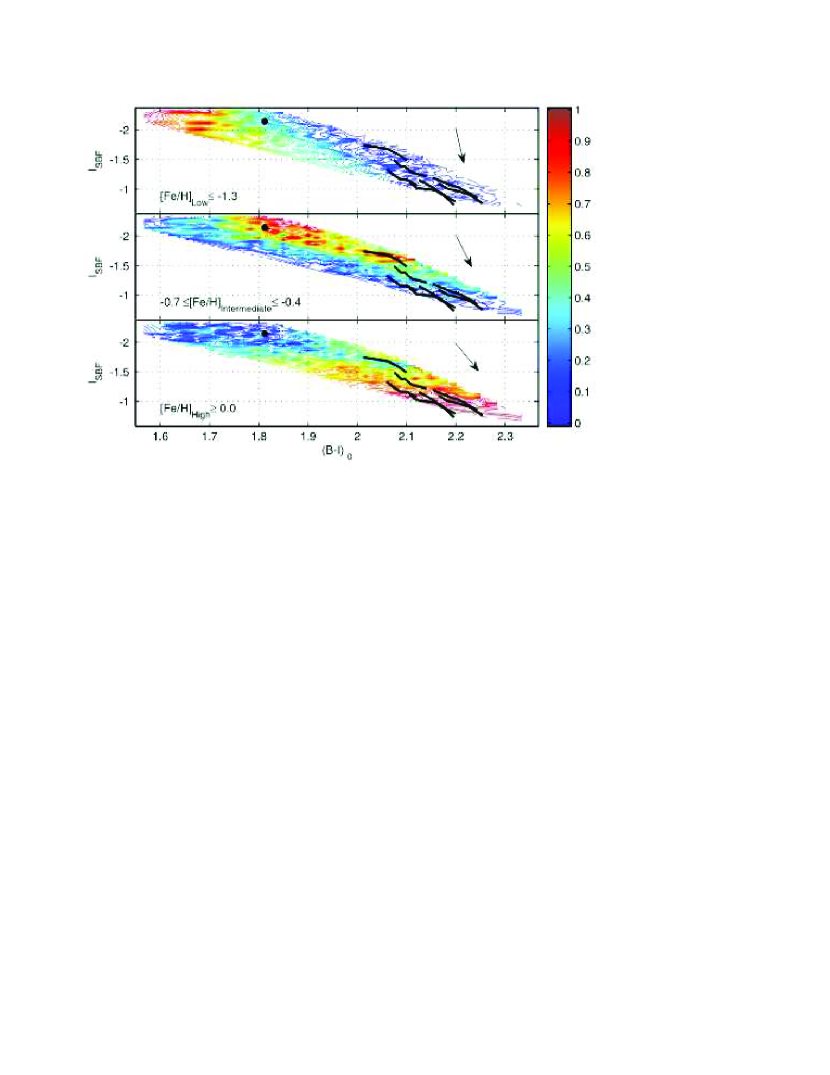
Figure 11: Composite stellar population models from BVA01, compared to observational data from this paper (solid black lines). For sake of clearness we have splitted the BVA01 composite models in three metallicity classes: low (upper panel), intermediate (middle panel), and high (lower panel) $[Fe/H]$ populations. The bar on the right shows the scale of colors associated to the relative weights (in %) of each one $[Fe/H]$-component in the model. That is, redder (bluer) colors indicate that the component is dominant (negligible) in the composite model. The spread in age affects mainly the $[Fe/H]_{\rm High}$ models which are computed for $4~{}Gyr\leq t\leq 18Gyr$, the $[Fe/H]_{\rm Low}$, $[Fe/H]_{\rm Intermediate}$ models are computed with ages ranging from 14 to 18 Gyr, and from 9 to 18 Gyr, respectively. The arrow in each panel indicates the direction of models with increasing age; the different slopes of arrows depict the different amplitudes of the age interval chosen for each metallicity class, i.e., steeper arrows correspond to narrower age intervals. See text for some more details on the figure.

All these data are plotted in Figure 5, which presents the measured $\bar{m}_{I}$ vs. $(B{-}I)_{0}$ profiles. With regards to this figure - and figures 7–11 - it is worth to note that brighter SBF magnitudes, and bluer $(B{-}I)_{0}$ colors correspond to outer galaxy’s regions.

3.3 Error Budget

Before concluding this section, we intend to discuss how the results obtained are affected by substantial changes of some of the assumption made. In particular we will discuss how variations in the (i) PSF, (ii) sky value, and in the (iii) luminosity function affect the estimated $\bar{m}_{I}$ and $(B{-}I)_{0}$.

(i) PSF - The ACS Point Spread Function shows to be stable enough in time. It is also fairly stable over the ACS field of view (Krist, 2003), with small spatial variation that is not significant for our analysis (Mei et al., 2005a).

The PSF used for this work comes from the ACS IDT, and is derived from the composition of several well isolated point sources obtained from other ACS observations. In order to study the sensitivity of the $P_{0}$ values to the PSF assumed, we fitted eq. (4) adopting three different PSFs, derived from individual high signal-to-noise stars in archival F814W ACS images. As a result we have obtained that the new $P_{0}$ derived agree within $2-3\%$ with the earlier values. Consequently, the final estimated $\bar{m}_{I}$ contains a systematic uncertainty due to the choice of the PSF, which is of the order of $0.03$ mag.

(ii) Sky - The estimation of sky background for the whole set of galaxies images is done under the assumption that the de Vaucouleurs $r^{1/4}$ profile describes the outer parts of the galaxy radial profile. However, such assumption may fail in the case of bright ellipticals, which are typically best fitted with a Sersic $r^{1/n}$ profile (Caon et al., 1993). We have verified how much the estimated sky would change if we assumed a $r^{1/n}$ profile. As a result we have that the changes are within $1~{}\sigma$ for the $n$=[3-8] range (which is still reasonable for these bright galaxies) but would go to $2~{}\sigma$ for $n$=2. Thus, we performed a test by changing the sky values within $2~{}\sigma$ the original value, the new values of $(B{-}I)_{0}$ and $\bar{m}_{I}$ measured agree within the associated uncertainty with the original measurements. Such variations are even less dramatic if the inner annuli are considered as well. Here, in fact, the sky to galaxy counts ratio is generally $\leq 0.05$, and the estimated original/perturbed colors and SBF agree under sky variations as high as $5~{}\sigma$ the original value.

(iii) Luminosity Function - To verify how the uncertainty in the fitted LF affects our results, we have performed several tests. First we have changed various SExtractor detection parameters, then we have also changed the convolution kernel for point sources detection (see Bertin & Arnouts 1996 for the details) and the parameters for the background subtraction. Finally, we have adopted a different routine to fit the LF, using the one from the ACS Virgo Cluster Survey which is optimized for dealing with ACS data. The resulting photometric catalogs differ from the original ones, but the final $\bar{m}_{I}$ values are well within $1~{}\sigma$ of the original measure. However, the result of this test is not surprising, since the high quality of ACS data allows to have an accurate photometric catalog of external sources down to the faintest magnitudes. Thus, the contamination due to undetected or low S/N sources is quite low, and residual $P_{r}$ does not give a major contribution to the fluctuations (compare the $\bar{m}_{I}^{uncorr.}$ and $\bar{m}_{I}$ values in column 6–7 of Table 3).

We have also tested how changing the slope $\gamma$ in the magnitude distribution of the background galaxies affects SBF magnitudes. For this test we used the $\gamma$ value determined by Benítez et al. (2004). As a result we have found that any detectable effect exists, the variation being well below $\sim 0.01$ mag. However, it must be emphasized that the $\gamma$ estimations from Bernstein et al. (2002), and Benítez et al. are consistent each other, and differ less than 5%.

Finally, to complete the list of uncertainties, it is worth noting that there is a $\sim 0.01$ mag error from the filter zeropoint, and a $\sim 0.01$ mag error from the flat fielding. To them we must add the mentioned uncertainty due to the transformation from ACS filter system to the standard system, which introduces a systematic error of $\sim 0.02$ ($\sim 0.01$, $\sim 0.03$) in $I$-band ($V$-, $B$-band) measurements.

4 Discussion

In the following sections we will discuss separately our SBF measurements as a tool to study distances, and to trace the properties of the dominant stellar populations of galaxies.

4.1 Calibration and Distances issues

The application of the SBF method as distance indicator relies on the calibration of $\bar{M}$ versus the galaxy broadband color (TAL90; Tonry et al. 1997). In our case we need to determine the slope $\beta$, and the zeropoint $\alpha$ of the equation:

$$\bar{M}_{I}=\alpha+\beta\cdot[(B-I)_{0}-2.0]$$ (7)

from the sample of available data. Figure 6 presents the complete dataset of measurements $\bar{m}_{I}$ vs. $(B{-}I)_{0}$ derived according to the procedures described in the preceding sections.

In order to determine the best values of $\alpha$, and $\beta$, we simultaneously fit all the galaxies of the sample, but NGC 404 for which we have no independent (radial) color information. The method applied to fit the unknown parameters of eq. (7) consists of the following steps. (a) Fix a lower limit value of $\beta$, then evaluate:

$$\langle\bar{m}_{I}\rangle_{j}=\langle\bar{m}_{I}^{(i)}-\beta\cdot[(B-I)_{0}^{(i)}-2.0]\rangle_{j}$$ (8)

by averaging over all annuli (index $i$) for each galaxy (index $j$). The value $\langle\bar{m}_{I}\rangle_{j}$ corresponds to the mean apparent fluctuation magnitude of the galaxy, at the fiducial color $(B{-}I)_{0}=2.0$ mag. Note that this quantity is strictly dependent on $\beta$. (b) Shift all galaxies to a common value of $\langle\bar{m}_{I}\rangle_{Reference}$ according to their $\langle\bar{m}_{I}\rangle_{j}$. (c) Calculate the $\chi^{2}$ over all annuli of all galaxies. (d) Increase $\beta$, and repeat the steps (a), (b), (c). The final value of the slope is assumed to be the one that minimizes the $\chi^{2}$ value (see Cantiello 2004 for full details; a similar approach is adopted in Tonry et al. 1997). As an illustration, Figure 7 exhibits the whole sample of data before (panel $a$) and after the shifting with three different values of $\beta$ (panels $b$, $c$, and $d$), keeping the NGC 1407 distance fixed. Adopting this procedure, we derive a best-fit value of $\beta=3.0$, shown in Figure 7$b$. To obtain a realistic estimate of the uncertainty of the slope, we perform a series of tests by applying a bootstrap method (Press et al., 1992). In conclusion the slope $\beta$ and its estimated uncertainty are $3.0\pm 0.3$.

Apart from determining $\beta$, the procedure applied allows to derive the relative distance moduli between our sample galaxies, without any assumption but the best value for $\beta$. In Table 4 we summarize the results obtained, taking NGC 1407 as reference galaxy.

Once we have evaluated $\beta$ and all relative distance moduli, to determine the zeropoint $\alpha$ we assume the Fornax cluster DM as reference – NGC 1344 being a member of this cluster. Adopting $DM_{Fornax}=31.5\pm 0.1$ (Ferrarese et al. 2000; T01; Blakeslee et al. 2002) we obtain: $\alpha=-1.6\pm 0.1$. Finally, we have:

$$\bar{M}_{I}=(-1.6\pm 0.1)+(3.0\pm 0.3)\cdot[(B-I)_{0}-2.0].$$ (9)

To test this result we compare it with the $I$-band calibration derived by Ajhar et al. (1997) for WFPC2 HST data. After applying the $(B{-}I)_{0}$-to-$(V{-}I)_{0}$ transformation equations reported in Appendix A (eq. A1), eq. (9) becomes:

$$\bar{M}_{I}=(-1.6\pm 0.2)+(6.5\pm 0.6)\cdot[(V-I)_{0}-1.15],$$ (10)

in fair agreement with the derivation by Ajhar et al.:

$$\bar{M}_{I}=(-1.73\pm 0.07)+(6.5\pm 0.7)\cdot[(V-I)_{0}-1.15].$$ (11)

Having fixed the Fornax Cluster DM as reference, we can also derive the galaxies’ absolute distance moduli from relative DM in Table 4. The resulting absolute DM are reported in column (3) of Table 4 ($DM_{This\,Work}$).

As a secondary check, we test our empirical calibration deriving the distance modulus of NGC 404. It must be pointed out that such application need to be considered with some cautions. In fact eq. (9) has been obtained for galaxies in the color range $2.00\leq(B-I)\leq 2.25$, while NGC 404 is outside this interval, having $(B{-}I)_{0}=1.81\pm 0.04$ mag. In spite of that, for this galaxy we derive $(\bar{m}_{I}-\bar{M}_{I})=27.59\pm 0.15$, in agreement with measurements from the ground based SBF survey ($27.57\pm 0.10$, T01), and with the estimation given by Tikhonov et al. (2003), who obtain $27.67\pm 0.15$ through the TRGB method.

On the theoretical side, adopting the Blakeslee et al. (2001, hereafter BVA01) stellar populations models in the age range $4-18~{}Gyr$, for metallicity $-0.4\leq[Fe/H]\leq 0.2$, and fitting a straight line to these data we find $\beta=3.5\pm 0.2$, and $\alpha=-1.75\pm 0.1$. While, considering their composite populations models, the value of $\beta$ can reach values down to $2.7\pm 0.2$, depending on the choice on the age and chemical properties of the stellar population mix (the zeropoint is left practically unchanged).

These results are confirmed by our new SBF models which give $\beta=3.3\pm 0.3$, and $\alpha=-1.7\pm 0.1$. The latter models are derived as described in Paper I, by using an upgraded set of evolutionary tracks (Pietrinferni et al., 2004) and a slightly different approach in considering the evolution of post-AGB stars (Paper II).

4.2 Stellar Populations issues

Combining SBF magnitudes and color data with synthetic stellar population models, one can infer information on the stellar content of galaxies (e.g., TAL90; Buzzoni 1993; Brocato et al. 1998; Worthey 1993; Blakeslee et al. 1999). Recent studies in this regard are broadly consistent with the view that ellipticals are generally not composed of a coeval, single metallicity stellar population (BVA01; Paper I; Jensen et al. 2003), supporting results given by spectrophotometric indicators (e.g., Kobayashi & Arimoto, 1999; Trager et al., 2000b, a).

The difficulty of using SBF as stellar population tracers, is the need of an independent estimation of the galaxy distance, if multi-band SBF measurements (that is SBF colors) are not available. However, having measured SBF magnitudes within various annuli of a single galaxy, we can study the radial behavior of the SBF vs. $(B{-}I)_{0}$ relation, or the radial SBF variations within each galaxy, in both cases the analysis of the relative changes is independent of galaxy distance. We divide the following discussion into distance independent and distance dependent analyses of the galaxy stellar populations.

4.2.1 Distance independent analysis: SBF–color relations and radial gradients

Radial gradients in broadband colors and line strength indices have long been used in the effort to constrain galaxy formation models (e.g., Strom et al., 1976; Cohen, 1979; Franx et al., 1989; Davies et al., 1993). This is because different formation histories can produce very different radial gradients. For instance, the traditional monolithic collapse scenario predicts steep inward metallicity gradients, which become more pronounced for more massive objects, while hierarchical merging models predict that radial gradients will flatten as galaxies undergo mergers; thus the most massive galaxies have shallower gradients because they experience the most merging (e.g., White, 1980; Bekki & Shioya, 2001; La Barbera et al., 2003, 2004). Thus, by characterizing the radial gradients in multiple stellar population indicators, it is possible to obtain useful information on a galaxy’s formation history.

Here, we consider the information provided on stellar population variations by our measured SBF and color gradients, and, in particular, from the slopes of the individual SBF–color relations. In § 4.1 we have derived an “overall” slope for the $\bar{M}_{I}$ vs. $(B{-}I)_{0}$ relation. The method applied to derive the value of $\beta$ allowed us to study this relation by using the SBF and color measurements of the whole sample of galaxies. The drawback in such a procedure is that it obscures the peculiarities of single objects. Here we intend to study each galaxy separately, pointing out the intrinsic differences among them, and suggesting the possible physical origin of these differences.

As can be recognized by eye inspection of Fig. 6, the slope of $\bar{M}_{I}$ vs. $(B{-}I)_{0}$, does not show strong variations on the whole set of plotted data. However, applying a weighted least squares method to derive the slope $\beta$ for each galaxy separately, some differences emerge. Table 5 list the slopes estimated, the reduced $\chi^{2}$, and the values of $q$ computed for single galaxies.

Two main considerations arise by inspecting the data in Table 5. First, there is a general agreement between these slopes within the quoted uncertainties. Moreover, with the exception of NGC 3258, all other listed values agree with the overall slope derived in the previous section. As discussed in more detail below, the steeper slope of the SBF-color relation in NGC 3258 would be appropriate for a pure metallicity gradient at fixed age, while the significantly shallower slope found for NGC 1344 requires some gradient in stellar population age. This is noteworthy because NGC 1344 is the bluest galaxy in our sample with the only exception of NGC 404, for which we do not have enough data to measure an SBF gradient; it also shows morphological irregularities indicative of recent merging activity (Carter et al., 1982). Since fractional age gradients will lessen with time (while metallicity gradients will remain fixed in the absence of further activity), it is reasonable that the SBF-color relation would suggest an age gradient in the youngest, bluest galaxy. Ultimately, we hope to correlate the slopes of SBF–color relations in large galaxy samples with other observables, including the local environment and other stellar population indicators, such as metal and Balmer absorption line strengths, in order to gain further insight into internal stellar population variations and enrichment histories.

4.2.2 Distance dependent analysis: absolute SBF magnitudes

To make a direct comparison of the single-band SBF data with predictions from models, we need to assume distance moduli for the galaxies. In Table 6 we report several distance moduli for each galaxy, estimated by using three different distance indicators: SBF (ground based measurements from T01), Fundamental Plane (FP), and distances derived from the IRAS redshift survey density field (the last two are from Blakeslee et al. 2002, see the paper for the details). Further, both single and group distances are considered. We show in Fig. 8 the location of our galaxy sample in the $\bar{M}_{I}$ vs. $(B{-}I)_{0}$ plane, against the various assumptions on the distance moduli. Clearly, the dispersion among the various derivations of distance moduli in Fig. 8 is quite high, in particular if single FP and SBF galaxy distances are used (panels $(b),(c)$).

On the other hand, considering group distances – which are expected to give a better estimation of the galaxy DM by averaging over the individual distance uncertainties – an interesting dichotomy appears to emerge. The galaxies NGC 3258, NGC 3268, NGC 4696, and NGC 5322, that is four among the farthest objects of the sample, lie on a fainter $\bar{M}_{I}$ vs. $(B{-}I)_{0}$ sequence than the galaxies NGC 1344 and NGC 1407 (and possibly NGC 404), the nearest objects of the sample (panels $(e),(f)$). This behavior could be due to the presence of some kind of bias in the DM estimated for the farthest objects or, more generally, to some kind of bias in the DM related to the distance of the objects. For example, by inspecting the quality parameters $Q$, and $PD$ reported by T01 for their SBF measurements, we find $Q/PD\geq 2.7$ for all the nearest galaxies, while it is $Q/PD\leq 0.7$ for the distant ones. Thus, we adopt the $IRAS$ group distances, that is: $\bar{M}_{I}=(\bar{m}_{I}-DM_{IRAS}^{Group})$. Note, however, that even assuming the IRAS distances there is still some dichotomy, in the sense that NGC 1344, and NGC 4696 still appear offset in this plane with respect to the other galaxies (Fig. 8, panel $(d)$). This suggests that the explanation may be a stellar population effect, rather than purely a relative distance error. In the following we will address this issue by comparing observational SBF and color data with theoretical predictions. Fig. 9 (left panel) compares SBF and color data from the present work with our new SBF models which are an upgraded version of the Paper I models for old metal-rich stellar populations (Cantiello 2004; Paper II); the right panel shows the models from BVA01. These two sets of models provide useful independent comparisons because they use different input stellar tracks, transformations to the empirical plane, and prescriptions for the later evolutionary phases. However, the implications of these independent models for the data are at least qualitatively similar.

As a general remark, we note that the innermost annuli of the galaxies have redder $(B{-}I)_{0}$ colors and fainter SBF magnitudes, with respect to the outer annuli. As shown also by the arrows in Fig. 9, simple age variations are expected to give shallower $\bar{M}_{I}$ vs. $(B{-}I)_{0}$ gradients with respect to chemical composition variation. Interestingly, the succession of the annular color-SBF measurements for individual galaxies in Fig. 9 follows preferentially the lines of increasing metallicity toward the center of the galaxy, with smaller changes in age. These results agree with the conclusions of many other authors (e.g., Trager et al., 2000b). More specifically, the results for NGC 1407, the Antlia group galaxies, and NGC 5322 agree with this general picture of the SBF and colour variations being driven by $[Fe/H]$ gradients, but for NGC 1344 the models indicate the presence of a younger stellar population in the outward from the center of the galaxy. As noted above, this behavior, which results in NGC 1344 having the smallest value for the SBF–color slope $\beta$, is consistent with the idea that NGC 1344 has undergone a merger or accretion event in the relatively recent past.

From inspection of both panels in Fig. 9, it appears that all the data for the giant galaxies are generally consistent with intermediate-age to old, metal-rich ($t\geq 5$ Gyr, $[Fe/H]\geq-0.3$) stellar populations. For NGC 404, the SBF–color data indicate a population of half solar metallicity and age $\lesssim 5$ Gyr, consistent with the results from the data/models comparison by Jensen et al. (2003), and the findings of Schmidt et al. (1990), though those authors analyze a smaller region. However, we caution that any detailed conclusions regarding absolute metallicities and ages depend on the assumed distance moduli. For instance, while the apparent dichotomy between NGC 1344 and the other galaxies can be explained by an offset of a factor of $\sim\,$3 in mean metallicity, this would require exclusively large ages of 9–13 Gyr in this galaxy. A younger age and more metal-rich population is found for this galaxy from optical–near-IR SBF colors (Jensen et al. 2003; Paper I) and line-strength analyses (Kuntschner et al., 2002), and would be more consistent with the indications of fairly recent merging.

To help illustrate the uncertainty further, we present in Figure 10 a comparison of the data with models assuming the average of the IRAS and FP group distances. In this case, the galaxy NGC 1407 is confirmed to host an old stellar population of nearly constant $t\sim 11$ Gyr, showing a significant increase of metal content in the innermost regions, while the implied age for NGC 4696 is reduced by nearly a factor of two. NGC 1344 is predicted to be dominated by a [Fe/H]${\,\ \raise-2.0pt\hbox{\hbox to0.0pt{\hbox{$\sim$}\hss}\raise 5.0pt\hbox{$>$}\ }\,}{-}0.3$ old population, but the disagreement with the results from the near-IR SBF and line-strength data is substantially reduced. The galaxies NGC 5322, NGC 3258 and NGC 3268, which are on average more massive than NGC 1407 and NGC 1344, remain consistent with an intermediate-to-old ($t\sim 5$–9 Gyr), super-solar metallicity stellar system.

As a final illustration of how such data could eventually be used to study stellar populations in more detail, we compare in Fig. 11 our observational data with the composite stellar population models presented by BVA01, assuming again the FP+IRAS average group distances. In addition to the $[Fe/H]$ interval considered in the preceding models, these composite models are computed by taking into account also a stellar component with metallicity in the range $-1.7\leq[Fe/H]\leq-0.4$. We split the BVA01 models into three metallicity classes, regardless of age: low (upper panel, $[Fe/H]_{\rm Low}$), intermediate (middle panel, $[Fe/H]_{\rm Intermediate}$), and high (lower panel, $[Fe/H]_{\rm High}$) metallicity populations. The spread in model age mainly comes in for the $[Fe/H]_{\rm High}$ component of the BVA01 models, which is computed by those authors for $4~{}Gyr\leq t\leq 18~{}Gyr$, while the $[Fe/H]_{\rm Low}$, and $[Fe/H]_{\rm Intermediate}$ components are computed with ages ranging from 14 to 18 Gyr, and from 9 to 18 Gyr, respectively.

The color coding (see the color bar on the right of the figure) shows the percentage of each $[Fe/H]$-component contributing to the composite population at a given point in the $\bar{M}_{I}$ vs. $(B{-}I)_{0}$ plane. For instance, red indicates that the particular region of the diagram would be populated by galaxies of mean metallicity equal to value for that particular panel, while blue indicates a negligible contribution from this metallicity component. As an example of the possible mixtures of populations able to reproduce the NGC 404 data in this diagram (black dot in Fig. 11), these composite models give a dominant stellar component intermediate in $[Fe/H]$ ($\sim$65% up to $\sim$90%), with a substantial contribution of low metallicity stars ($\sim$15% to $\sim$40%), and a very low percentage of high $[Fe/H]$ stars ($\sim$0% to $\sim$25%). However, the mix of populations needed to reproduce a given point in the $\bar{M}_{I}$ vs. $(B{-}I)_{0}$ plane is not unique, and additional observables (e.g., optical and near-IR SBF colors) are needed to achieve firm, distance-independent constraints on composite stellar population modeling.

5 Summary

We have presented a photometric study of eight ellipticals imaged with the ACS camera on board of HST. Classical broad-band $(B{-}I)_{0}$ colors, $B$-, $I$-band magnitudes, and $I$-band SBF magnitudes are determined for each galaxy.

Given the exceptional resolution of the ACS camera, we succeeded in measuring SBF and integrated color gradients within galaxies. This has allowed us to study the slope of the $\bar{M}_{I}$ vs. $(B{-}I)_{0}$ relation in a quite different way compared to earlier applications. Previous studies derived the slope analyzing multiple galaxies within the same group, that is, assuming the cluster depth to be negligible compared to the distance from the observer. The data analysis presented in this work does not rely on any assumption about group or cluster scatter, and shows that, by using galaxy internal SBF gradients, the uncertainty in the $\bar{M}_{I}$ vs. $(B{-}I)_{0}$ slope can be substantially reduced.

We derive the zeropoint of the empirical $\bar{M}_{I}$ vs. $(B{-}I)_{0}$ relation using our measurements for NGC 1344 (a member of the Fornax cluster) combined with the known Cepheid distance to Fornax, and thus present the first full empirical calibration of the $I$-band SBF method for the ACS instrument.

Concerning the use of SBF as tracer of stellar population properties, our results substantially confirm the generally well established view of ellipticals as complex objects, typically dominated by an old, [Fe/H]$\geq-0.3$ stellar population. SBF radial gradients are introduced as a new inquiry tool. In particular, inspection of the SBF and color gradients in comparison to models suggests that radial changes are preferentially due to chemical composition changes, more than to age, with the outer regions of galaxies being more metal poor than the innermost regions. Assuming the distance of galaxies from other indicators, we show that the theory/observations comparison in the $\bar{M}_{I}$ vs. $(B{-}I)_{0}$ plane can help to disentangle the age/metallicity degeneracy. While the limited data sample precludes any firm conclusions, we consider the results of this study promising for future investigations of galaxy enrichment histories incorporating SBF and color gradients.

Appendix A Transforming $(B{-}I)_{0}$ into $(V{-}I)_{0}$, and vice versa

The main body of the data used for this work consisted of F814W, and F435W long exposures of low redshift bright ellipticals. Since for the other two galaxies – NGC 404 and NGC 1344 – no F435W data are available, in order to make an homogeneous comparison with the other galaxies we needed to derive their $(B{-}I)_{0}$ color from the available V and I band data.

For NGC 1344, an exposure in the F606W filter is available from the same proposal, thus we determined the $(F606W{-}F814W)_{0}$ radial profile for this galaxy, then $(F606W{-}F814W)_{0}$ was transformed into the standard $(V{-}I)_{0}$ by using the S05 transformations, finally $(V{-}I)_{0}$ was in turn transformed to $(B{-}I)_{0}$. For NGC 404 we only had an F814W image, consequently the $(B{-}I)_{0}$ color was derived from the $(V{-}I)_{0}$ measurement for this galaxy given by T01.

In both cases the $(V{-}I)_{0}$–to–$(B{-}I)_{0}$ transformation equations are derived from the upgraded version of the Cantiello et al. (2003) stellar populations models, by fitting a straight line to the $(B{-}I)_{0}$-$(V{-}I)_{0}$ theoretical predictions for simple stellar populations in the age range $5~{}{\rm Gyr}\leq t\leq 15$ Gyr, and in the metallicity range $-0.3\leq[Fe/H]\leq 0.3$. The fitted equations are:

$$(B-I)_{Transf}=(2.15\pm 0.02)\cdot(V-I)_{0}+(-0.45\pm 0.02).$$ (A1)

To check the reliability of this transformation, the $(V{-}I)_{0}$ measurements from T01 are transformed to $(B{-}I)_{0}$ applying eq. (A1), the resulting $(B-I)_{Transf.}$ is then compared to $(B{-}I)_{0}$ from this paper.

The result of the comparison can be found in Tab. 7, and Fig. 12. Quoted in the table there are: (1) the galaxy name, (2) average radius of the annulus contributing to color measurement, the ratio of the innermost to average radius, the ratio of the outermost to average radius contributing to the mean color; (3) the measured $(B{-}I)_{0}$ color; (4) $(V{-}I)_{0}$ color from by T01; (5) $(B-I)_{Transf.}$ color obtained applying eq. (A1).

For sake of completeness we report here the $(B{-}I)_{0}$-$(V{-}I)_{0}$ color transformations as predicted by using the BVA01 and the Bruzual & Charlot (2003, BC03 - their Padua 1994 isochrones and Salpeter IMF) models for Simple Stellar Populations (only populations with $5~{}{\rm Gyr}\leq t\leq 15$ and $-0.4\leq[Fe/H]\leq 0.4$ are considered):

$$(B-I)_{0}^{BVA01}=(2.06\pm 0.02)\cdot(V-I)_{0}+(-0.32\pm 0.03),$$ (A2)

$$(B-I)_{0}^{BC03}=(2.09\pm 0.02)\cdot(V-I)_{0}+(-0.39\pm 0.03).$$ (A3)

At the fiducial color $(V{-}I)_{0}=1.15$, the three different transformation equations (A1, A2, A3) predict $(B{-}I)_{0}$ color equal to 2.02$\pm$0.03, 2.06$\pm$0.04, 2.02$\pm$0.04 (respectively: our, BVA01, and BC03 models). However, even such small variations can determine non-negligible differences in some of the applications presented in this work. As an example, the transformation of eq. (9) [§ 4.1, $\bar{M}_{I}$ vs. $(B{-}I)_{0}$] into eq. (10) [$\bar{M}_{I}$ vs. $(V{-}I)_{0}$] changes significantly according to the set of models that is used:

$$\bar{M}_{I}^{BVA01}=(-1.6\pm 0.2)+(6.2\pm 0.6)\cdot[(V-I)_{0}-1.15],$$ (A4)

and

$$\bar{M}_{I}^{BC03}=(-1.6\pm 0.3)+(6.3\pm 0.6)\cdot[(V-I)_{0}-1.15].$$ (A5)

Note that results from eqs. A4, A5, and 10 still agree with each other at the $1~{}\sigma$ level. Interestingly, the zeropoints of equations 10, A4, and A5 nicely reproduce the $\bar{M}_{I}$ vs. $(V{-}I)_{0}$ zeropoint derived by Tonry et al. (2000) by using group distances (as a matter of fact, combining all models we find $\bar{M}_{I}^{(V{-}I)_{0}=1.15}=-1.6\pm 0.1$, to be compared with the observationally derived $-1.61\pm 0.03$).

The sequence of frames used for the photometry/SBF analysis (the case of NGC 1407 is shown). The upper two panels show the original image (left) and the galaxy model (right), using a logarithmic stretch. The lower panels show the galaxy-subtracted frame (left) and the final residual frame (right), shown using a simple linear gray scale. The rich globular cluster populations can be easily seen after the galaxy model is subtracted (lower left panel). In the lower right panel the external sources visible in the galaxy-subtracted image are masked out, the fluctuations are clearly visible in the “bumpiness” near the center of this panel.

Figure 1: Panels (a) - Open squares: I band surface brightness profile. Open triangles: the same for $B$ band ($V$ band for NGC 1344). Panels (b) - Measured $(B{-}I)_{0}$ profile as a function of radius. Error bars are also shown as thin solid lines. Data are corrected for Galactic extinction, and plotted against the (fourth root of the) semi-major axis of the isophote. Note that for NGC 1344 the $(V{-}I)_{0}$ color profile is plotted.

Figure 2: Difference of the measured Surface Brightness profile and the $r^{1/4}$ profile fitted in the outer regions of the galaxies ($\Delta\mu=\mu_{observed}-\mu_{r^{1/4}fit}$), plotted against galaxy radius. Left (right) panels: I (B) band profile differences.

Figure 3: The fitted Luminosity Function of external sources. Open squares mark observational data, the solid line represent the best fit of the data. The LF of background galaxies and globular clusters are plotted as a dotted and a dashed line, respectively.

Figure 4: NGC 1407 power spectrum analysis. In the upper panels we plot the azimuthal average of the residual image power spectrum (dots), and the fit obtained according to the procedure described in text (solid line). The original images were processed in the same way, but with different drizzle kernels: Point kernel (left panels), and Lancosz3 kernel (right panels). The lower panels show the fitted $P_{0}$ as a function of the starting wavenumber of the fit, $P_{0}(k_{fit}>k)$. The weighted average of the values in the flatter $P_{0}$ vs. $k$ region ($100\ \raise-2.0pt\hbox{\hbox to0.0pt{\hbox{$\sim$}\hss}\raise 5.0pt\hbox{$<$}\ }k\ \raise-2.0pt\hbox{\hbox to0.0pt{\hbox{$\sim$}\hss}\raise 5.0pt\hbox{$<$}\ }300$), is taken to derive the final $P_{0}$ value and its uncertainty. This last data is then adopted to evaluate the final $\bar{m}_{I}$, quoted in figure. All plots refer to the same image annulus ($20^{\prime\prime}\ \raise-2.0pt\hbox{\hbox to0.0pt{\hbox{$\sim$}\hss}\raise 5.0pt\hbox{$<$}\ }r\ \raise-2.0pt\hbox{\hbox to0.0pt{\hbox{$\sim$}\hss}\raise 5.0pt\hbox{$<$}\ }25^{\prime\prime}$).

Figure 5: SBF amplitudes measured in the various galaxy annuli plotted against the $(B{-}I)_{0}$ color of the annulus. Note that while the $(B{-}I)_{0}$ color in Fig. 1 has been evaluated in annuli with semi-major length: $(r_{out}-r_{in})\sim 16$ pixels ($\sim 32$ pixels for the outermost regions), the annuli adopted to evaluate the $(B{-}I)_{0}$ plotted in this figure are the same used for SBF evaluation, that is $(r_{in},r_{out})$=[(128, 256), (257, 384), (385, 512), (513, 768), (769, 1024)] in pixel units. We advise that in the panels of this figure (as well as in Fig. 7–11) brighter fluctuations magnitudes, and bluer $(B{-}I)_{0}$ colors in general correspond to more external annuli. For sake of clearness the plotted axis range is different for each of the three blocks in the figure, according to the observed ranges of $(B{-}I)_{0}$ and $\bar{m}_{I}$ for the galaxies, though we keep fixed the amplitude of the intervals. Concerning NGC 1344 see Appendix A for the color equations adopted to obtain the $(B{-}I)_{0}$ from the measured $(V{-}I)_{0}$.

Figure 6: The distribution of apparent SBF magnitudes versus galaxy color. NGC 404 is not displayed for the clearness of the plot, it is located at [$(B{-}I)_{0}\sim 1.81$, $\bar{m}_{I}\sim-2.2$].

Figure 7: Panel $(a)$ - The observed distribution of $\bar{m}_{I}$ vs. $(B{-}I)_{0}$ data for the whole sample of galaxies, but NGC 404. Panel $(b)$ - Observational data are shifted to the reference (relative) distance of NGC 1407. The best fit to the data is plotted as a dashed line. The value of $\beta$ assumed for the shifting is reported too. Panels $(c)$, and $(d)$ - similar to panel $(b)$ but for different $\beta$ values. Our best estimation of the slope is $\beta\sim 3$ (panel $b$). By comparing the $(b)$, $(c)$, and $(d)$ panels, it can be seen how the minimization procedure works: the best fit value of $\beta$ is the one that minimizes the scatter of observational data with the expected linear dependence.

Figure 8: The distribution of the absolute SBF magnitudes as a function of $(B{-}I)_{0}$. Each panel refers to a different assumption on the distance modulus (upper left quote). Left panels refer to the distances derived for the single object, right panels to group average distances (for some useful notes on group definitions see T01). Symbols are the same of Fig. 6. For NGC 404 (full triangle at $(B{-}I)_{0}\sim 1.81$, $\bar{m}_{I}\sim 25.4$) no group distance is assumed, the SBF distance modulus is adopted in all cases.

Figure 9: Absolute $\bar{M}_{I}$ magnitude derived assuming the IRAS group distances (in all cases but NGC 404; see text for details) versus the measured $(B{-}I)_{0}$ of the sample. Left panel - Our new SBF models, for [5,7,9,11,13,15] Gyr and three different metallicities: $[Fe/H]=-0.3,~{}0.0,~{}+0.3$. Models of increasing age are marked with symbols of increasing size, the direction of the increase is shown by the “Age” arrow. Also indicated by the dashed arrow is the direction of increasing metallicity [Fe/H]. Symbols for observational data are the same of Fig. 6, NGC 404 is marked with a full triangle. The case of NGC 5557 is not considered since no group distance is known for this galaxy (Table 6). The median error bars are indicated lower right in the panel. Right panel - The same as before, but for BVA01 models, for ages ranging from 5 Gyr to 17.8 (increasing in steps of 12%) and metallicities: $[Fe/H]=-0.4,~{}0.0,~{}+0.2$.

Figure 10: As Fig. 9 but for average IRAS+FP group distances (see text).

Figure 12: Left panel - Distribution of theoretical prediction for old ($t\geq 5~{}Gyr$), $[Fe/H]\geq-0.3$ stellar populations in the $(B{-}I)_{0}$-$(V{-}I)_{0}$ plane. Dashed lines are upgraded version of Cantiello et al. (2003) models of simple stellar populations, also the best fit line is plotted. Full dots refer to $(B{-}I)_{0}$ measurements from this work, and to $(V{-}I)_{0}$ data from T01 (data measured within the same galaxy’s region). Right panel - $(B-I)_{Transf}$ color derived applying eq. (A1) to the $(V{-}I)_{0}$ measured by T01, versus $(B{-}I)_{0}$ measured in this work. The dashed line is not a fit of the data.

Table 1: Observational Data

Galaxy	Group	R.A.	Decl.	$v_{cmb}$	T	$A_{B}$	Prog.	Exp. time	Other ACS	Exp.
	(group #)			($km/s$)			ID#	F814W ($s$)	Filter	time ($s$)
NGC 1407	Eridanus (32)	55.052	-18.581	1627	-5	0.297	9427	680	F435W	1500
NGC 3258	Antlia (46)	157.226	-35.606	3129	-5	0.363	9427	2280	F435W	5360
NGC 3268	Antlia (46)	157.503	-35.325	3084	-5	0.444	9427	2280	F435W	5360
NGC 4696	Centaurus (58)	192.208	-41.311	3248	-4	0.489	9427	2320	F435W	5440
NGC 5322	NGC 5322 (254)	207.315	60.191	1916	-5	0.061	9427	820	F435W	3390
NGC 5557	$\cdots$ (228)	214.605	36.494	3433	-5	0.025	9427	2400	F435W	5260
NGC 404	$\cdots$ (0)	17.363	35.718	-332	-3	0.253	9293	700	$\cdots$	$\cdots$
NGC 1344	Fornax (31)	52.080	-31.068	1086	-5	0.077	9399	960	F606W	1062

Table 2: Parameters used for the Detection, Background estimation, and Deblending with SExtractor v2.2.2

Parameter	Value
BACK_SIZE	128
BACK_FILTERSIZE	5
CLEAN	Y
CLEAN_PARAM	1.5
DETECT_MINAREA	5
DETECT_THRESH	1.5
DEBLEND_NTHRESH	8
DEBLEND_MINCONT	0.008
FILTER	Y
FILTER_NAME	gauss_2.0_3x3.conv
PHOT_APERTURES	6
WEIGHT_TYPE	MAP_RMS
WEIGHT_THRESH	0, 1.0e30
BACK_SIZE	25
BACK_FILTERSIZE	3

Table 3: Color & SBF measured in each annulus for the whole sample of galaxies. All data are extinction corrected.

Annulus	$\langle r(arcsec)\rangle$	$e$	$(B-I)_{0}$	$\bar{m}_{I}^{uncorr.}$	$\bar{m}_{I}$
NGC1407
1	10	0.05	2.244 0.003	31.01	31.15 0.05
2	16	0.05	2.219 0.006	30.94	31.02 0.03
3	22	0.05	2.205 0.009	30.90	30.97 0.03
4	32	0.04	2.188 0.015	30.86	30.92 0.02
5	43	0.04	2.153 0.025	30.74	30.80 0.02
NGC3258
1	9	0.14	2.196 0.004	31.99	32.08 0.04
2	15	0.10	2.169 0.010	31.80	31.86 0.03
3	22	0.08	2.156 0.019	31.75	31.82 0.03
4	31	0.08	2.120 0.035	31.70	31.78 0.02
5	42	0.10	2.105 0.060	31.58	31.68 0.03
NGC3268
1	9	0.19	2.199 0.005	31.93	32.02 0.03
2	15	0.20	2.165 0.011	31.80	31.87 0.03
3	20	0.21	2.159 0.018	31.75	31.81 0.02
4	29	0.21	2.140 0.030	31.66	31.71 0.02
5	40	0.22	2.125 0.050	31.56	31.65 0.02
NGC4696
1	11	0.14	2.254 0.004	31.97	32.16 0.06
2	15	0.15	2.229 0.006	31.91	32.02 0.04
3	21	0.16	2.208 0.008	31.88	31.96 0.03
4	30	0.17	2.183 0.013	31.83	31.91 0.03
5	38	0.19	2.165 0.018	31.75	31.82 0.02
NGC5322
1	8	0.31	2.120 0.002	31.19	31.38 0.06
2	14	0.30	2.100 0.003	31.20	31.28 0.03
3	19	0.31	2.087 0.005	31.22	31.29 0.03
4	28	0.32	2.069 0.009	31.13	31.18 0.02
5	37	0.34	2.060 0.016	31.07	31.12 0.02
NGC5557
1	9	0.19	2.141 0.004	32.16	32.24 0.04
2	15	0.16	2.111 0.009	32.11	32.17 0.03
3	21	0.16	2.096 0.014	32.02	32.07 0.02
4	30	0.15	2.089 0.025	32.01	32.07 0.02
5	41	0.14	2.075 0.051	31.89	31.96 0.02
NGC1344
1	9	0.30	2.10 0.02	30.04	30.17 0.04
2	14	0.31	2.08 0.02	30.04	30.08 0.02
3	19	0.34	2.06 0.02	29.96	29.98 0.01
4	27	0.37	2.04 0.02	29.94	29.95 0.01
5	37	0.38	2.01 0.03	29.91	29.92 0.01
NGC404
1	10	0.08	1.81 0.03	$\cdots$	25.42 0.01
2	16	0.06	1.81 0.03	$\cdots$	25.39 0.01
3	22	0.07	1.81 0.03	$\cdots$	25.43 0.01
4	31	0.08	1.81 0.03	$\cdots$	25.45 0.01
5	42	0.09	1.81 0.03	$\cdots$	25.45 0.01

Table 4: Galaxies relative and absolute distance moduli

Galaxy	$\Delta DM$	$DM_{This\,Work}$	$\langle DM_{Single}\rangle$	$\langle DM_{Group}\rangle$
NGC1407	0.0	32.0 $\pm$ 0.1	32.1 $\pm$ 0.15	32.01 $\pm$ 0.05
NGC3258	1.0 $\pm$ 0.1	33.0 $\pm$ 0.15	33.0 $\pm$ 0.15	32.8 $\pm$ 0.1
NGC3268	1.0 $\pm$ 0.1	33.0 $\pm$ 0.15	32.9 $\pm$ 0.15	32.8 $\pm$ 0.1
NGC4696	1.0 $\pm$ 0.09	33.0 $\pm$ 0.1	32.8 $\pm$ 0.15	32.86 $\pm$ 0.04
NGC5322	0.6 $\pm$ 0.08	32.6 $\pm$ 0.1	32.4 $\pm$ 0.15	32.4 $\pm$ 0.1
NGC5557	1.4 $\pm$ 0.1	33.4 $\pm$ 0.15	33.4 $\pm$ 0.1	$\cdots$
NGC1344	-0.5 $\pm$ 0.15	$\cdots$	31.5 $\pm$ 0.3	31.53 $\pm$ 0.03

Table 5: Slope fitted for single galaxy

Galaxy	$\beta$	$\chi^{2}$	$q$
NGC1407	3.8 $\pm$ 1.1	0.333	0.954
NGC3258	6.4 $\pm$ 2.0	1.014	0.798
NGC3268	4.7 $\pm$ 1.4	0.063	0.996
NGC4696	3.3 $\pm$ 0.9	0.945	0.815
NGC5322	3.9 $\pm$ 1.0	1.568	0.667
NGC5557	3.5 $\pm$ 1.0	0.935	0.817
NGC1344	3.0 $\pm$ 2.2	0.252	0.969

Table 6: Distance Moduli assumed to derive the galaxies’ SBF absolute magnitudes

Galaxy	$SBF_{T01}$	$FP_{B02}$	$IRAS_{REF}$	$SBF_{T01}$	$N_{SBF}$	$FP_{B02}$	$IRAS_{REF}$	$N_{FP+IRAS}$
	Single Distances			Group Distances
NGC1407	32.30 $\pm$ 0.26	31.96 $\pm$ 0.41	32.04 $\pm$ 0.24	32.00 $\pm$ 0.08	7	32.04 $\pm$ 0.08	31.95 $\pm$ 0.11	5
NGC3258	32.53 $\pm$ 0.27	33.73 $\pm$ 0.41	33.00 $\pm$ 0.19	32.64 $\pm$ 0.15	3	32.63 $\pm$ 0.18	32.98 $\pm$ 0.14	2
NGC3268	32.71 $\pm$ 0.25	33.34 $\pm$ 0.41	32.97 $\pm$ 0.19	32.64 $\pm$ 0.15	3	32.63 $\pm$ 0.18	32.98 $\pm$ 0.14	2
NGC4696	32.75 $\pm$ 0.17	32.19 $\pm$ 0.41	33.12 $\pm$ 0.24	32.64 $\pm$ 0.08	9	32.64 $\pm$ 0.08	33.19 $\pm$ 0.07	9
NGC5322	32.47 $\pm$ 0.23	31.74 $\pm$ 0.41	32.46 $\pm$ 0.20	32.29 $\pm$ 0.15	4	32.34 $\pm$ 0.19	32.55 $\pm$ 0.13	2
NGC5557	$\cdots$	32.92 $\pm$ 0.41	33.49 $\pm$ 0.11	$\cdots$	$\cdots$	$\cdots$	$\cdots$	$\cdots$
NGC404	27.57 $\pm$ 0.10	$\cdots$	$\cdots$	$\cdots$	$\cdots$	$\cdots$	$\cdots$	$\cdots$
NGC1344	31.48 $\pm$ 0.30	$\cdots$	$\cdots$	31.49 $\pm$ 0.04	26	31.55 $\pm$ 0.06	31.76 $\pm$ 0.10	9

Table 7: $(B-I)_{0}$ to $(V-I)_{0}$ transformations

Galaxy	$\langle r\rangle$	$(V-I)_{0}$	$(V-I)_{0}^{T01}$	$(B-I)_{Transf.}$
NGC404	23 0.0 3.8	$\cdots$	1.054 $\pm$ 0.011	1.812 $\pm$ 0.034
NGC1344	27 0.3 2.2	1.150 $\pm$ 0.025	1.135 $\pm$ 0.011	1.986 $\pm$ 0.034
Galaxy            $\langle r\rangle$          $(B-I)_{0}$        $(V-I)_{0}^{T01}$      $(B-I)_{Transf.}$
NGC1407	31 0.2 1.9	2.188 $\pm$ 0.029	1.232 $\pm$ 0.018	2.173 $\pm$ 0.033
NGC3258	26 0.3 2.3	2.163 $\pm$ 0.069	1.220 $\pm$ 0.036	2.145 $\pm$ 0.077
NGC3268	9 0.5 1.9	2.193 $\pm$ 0.012	1.235 $\pm$ 0.012	2.102 $\pm$ 0.056
NGC4696	57 0.3 2.1	2.181 $\pm$ 0.067	1.229 $\pm$ 0.035	2.132 $\pm$ 0.039
NGC5322	29 0.4 3.0	2.070 $\pm$ 0.036	1.174 $\pm$ 0.020	2.089 $\pm$ 0.034
NGC5557	25 0.2 1.7	2.113 $\pm$ 0.017	1.195 $\pm$ 0.013	2.130 $\pm$ 0.052

References

- Ajhar et al. (1997) Ajhar, E. A., Lauer, T. R., Tonry, J. L., Blakeslee, J. P., Dressler, A., Holtzman, J. A., & Postman, M. 1997, AJ, 114, 626
- Ajhar & Tonry (1994) Ajhar, E. A., & Tonry, J. L. 1994, ApJ, 429, 557
- Baade (1944) Baade, W. 1944, ApJ, 100, 137
- Bekki & Shioya (2001) Bekki, K., & Shioya, Y. 2001, Ap&SS, 276, 767
- Benítez et al. (2004) Benítez, N. et al. 2004, ApJS, 150, 1
- Bernardi et al. (2003) Bernardi, M. et al. 2003, AJ, 125, 1882
- Bernstein et al. (2002) Bernstein, R. A., Freedman, W. L., & Madore, B. F. 2002, ApJ, 571, 107
- Bertin & Arnouts (1996) Bertin, E., & Arnouts, S. 1996, A&AS, 117, 393
- Blakeslee et al. (1999) Blakeslee, J. P., Ajhar, E. A., & Tonry, J. L. 1999, in ASSL Vol. 237: Post-Hipparcos cosmic candles, 181–+
- Blakeslee et al. (2003) Blakeslee, J. P., Anderson, K. R., Meurer, G. R., Benítez, N., & Magee, D. 2003, in ASP Conf. Ser. 295: Astronomical Data Analysis Software and Systems XII
- Blakeslee et al. (2002) Blakeslee, J. P., Lucey, J. R., Tonry, J. L., Hudson, M. J., Narayanan, V. K., & Barris, B. J. 2002, MNRAS, 330, 443
- Blakeslee et al. (2001) Blakeslee, J. P., Vazdekis, A., & Ajhar, E. A. 2001, MNRAS, 320, 193 (BVA01)
- Brocato et al. (1998) Brocato, E., Capaccioli, M., & Condelli, M. 1998, Memorie della Societa Astronomica Italiana, 69, 155
- Bruzual & Charlot (2003) Bruzual, G., & Charlot, S. 2003, MNRAS, 344, 1000 (BC03)
- Buzzoni (1993) Buzzoni, A. 1993, A&A, 275, 433
- Cantiello (2004) Cantiello, M. 2004, PhD Thesis, University of Salerno, Salerno, Italy
- Cantiello et al. (2003) Cantiello, M., Raimondo, G., Brocato, E., & Capaccioli, M. 2003, AJ, 125, 2783 (Paper I)
- Caon et al. (1993) Caon, N., Capaccioli, M., & D’Onofrio, M. 1993, MNRAS, 265, 1013
- Carter et al. (1982) Carter, D., Allen, D. A., & Malin, D. F. 1982, Nature, 295, 126
- Cimatti et al. (2004) Cimatti, A. et al. 2004, Nature, 430, 184
- Cohen (1979) Cohen, J. G. 1979, ApJ, 228, 405
- Davies et al. (1993) Davies, R. L., Sadler, E. M., & Peletier, R. F. 1993, MNRAS, 262, 650
- Faber et al. (1989) Faber, S. M., Wegner, G., Burstein, D., Davies, R. L., Dressler, A., Lynden-Bell, D., & Terlevich, R. J. 1989, ApJS, 69, 763
- Ferrarese et al. (2000) Ferrarese, L. et al. 2000, ApJ, 529, 745
- Ford et al. (1998) Ford, H. C. et al. 1998, in Proc. SPIE Vol. 3356, p. 234-248, Space Telescopes and Instruments V, Pierre Y. Bely; James B. Breckinridge; Eds., 234–248
- Ford et al. (2003) Ford, H. C. et al. 2003, in Future EUV/UV and Visible Space Astrophysics Missions and Instrumentation. Edited by J. Chris Blades, Oswald H. W. Siegmund. Proceedings of the SPIE, Volume 4854, pp. 81-94 (2003)., 81–94
- Franx et al. (1989) Franx, M., Illingworth, G., & Heckman, T. 1989, AJ, 98, 538
- Fruchter & Hook (2002) Fruchter, A. S., & Hook, R. N. 2002, PASP, 114, 144
- González et al. (2004) González, R. A., Liu, M. C., & Bruzual A., G. 2004, ApJ, 611, 270
- Goudfrooij et al. (1994) Goudfrooij, P., Hansen, L., Jorgensen, H. E., & Norgaard-Nielsen, H. U. 1994, A&AS, 105, 341
- Harris (1991) Harris, W. E. 1991, ARA&A, 29, 543
- Harris (2001) Harris, W. E. 2001, in Saas-Fee Advanced Course 28: Star Clusters
- Henry & Worthey (1999) Henry, R. B. C., & Worthey, G. 1999, PASP, 111, 919
- Jacoby et al. (1992) Jacoby, G. H. et al. 1992, PASP, 104, 599
- Jedrzejewski (1987) Jedrzejewski, R. I. 1987, MNRAS, 226, 747
- Jensen et al. (2003) Jensen, J. B., Tonry, J. L., Barris, B. J., Thompson, R. I., Liu, M. C., Rieke, M. J., Ajhar, E. A., & Blakeslee, J. P. 2003, ApJ, 583, 712
- Jensen et al. (1998) Jensen, J. B., Tonry, J. L., & Luppino, G. A. 1998, ApJ, 505, 111
- Jensen et al. (2001) Jensen, J. B., Tonry, J. L., Thompson, R. I., Ajhar, E. A., Lauer, T. R., Rieke, M. J., Postman, M., & Liu, M. C. 2001, ApJ, 550, 503
- Kobayashi (2004) Kobayashi, C. 2004, MNRAS, 347, 740
- Kobayashi & Arimoto (1999) Kobayashi, C., & Arimoto, N. 1999, ApJ, 527, 573
- Kormendy & Djorgovski (1989) Kormendy, J., & Djorgovski, S. 1989, ARA&A, 27, 235
- Krist (2003) Krist, J. 2003, , Tech. rep., Instrument Science Report ACS 2003-06
- Kuntschner et al. (2002) Kuntschner, H., Smith, R. J., Colless, M., Davies, R. L., Kaldare, R., & Vazdekis, A. 2002, MNRAS, 337, 172
- La Barbera et al. (2003) La Barbera, F., Busarello, G., Massarotti, M., Merluzzi, P., & Mercurio, A. 2003, A&A, 409, 21
- La Barbera et al. (2004) La Barbera, F., Merluzzi, P., Busarello, G., Massarotti, M., & Mercurio, A. 2004, A&A, 425, 797
- Liu et al. (2002) Liu, M. C., Graham, J. R., & Charlot, S. 2002, ApJ, 564, 216
- Mei et al. (2005a) Mei, S. et al. 2005a, ApJS, 156, 113
- Mei et al. (2005b) —. 2005b, ApJ, 625, 121
- Mei et al. (2001) Mei, S., Silva, D. R., & Quinn, P. J. 2001, A&A, 366, 54
- Pagel & Edmunds (1981) Pagel, B. E. J., & Edmunds, M. G. 1981, ARA&A, 19, 77
- Peebles (2002) Peebles, P. J. E. 2002, in ASP Conf. Ser. 283: A New Era in Cosmology
- Pietrinferni et al. (2004) Pietrinferni, A., Cassisi, S., Salaris, M., & Castelli, F. 2004, ApJ, 612, 168
- Press et al. (1992) Press, W. H., Teukolsky, S. A., Vetterling, W. T., & Flannery, B. P. 1992, Numerical recipes in FORTRAN. The art of scientific computing (Cambridge: University Press, —c1992, 2nd ed.)
- Raimondo et al. (2005) Raimondo, G., Brocato, E., Cantiello, M., & Capaccioli, M. 2005, AJ submitted (Paper II)
- Renzini & Cimatti (1999) Renzini, A., & Cimatti, A. 1999, in ASP Conf. Ser. 193: The Hy-Redshift Universe: Galaxy Formation and Evolution at High Redshift
- Schlegel et al. (1998) Schlegel, D. J., Finkbeiner, D. P., & Davis, M. 1998, ApJ, 500, 525
- Schmidt et al. (1990) Schmidt, A. A., Bica, E., & Alloin, D. 1990, MNRAS, 243, 620
- Sirianni et al. (2005) Sirianni, M. et al. 2005, PASP accepted (S05)
- Stetson (1990) Stetson, P. B. 1990, PASP, 102, 932
- Strom et al. (1976) Strom, S. E., Strom, K. M., Goad, J. W., Vrba, F. J., & Rice, W. 1976, ApJ, 204, 684
- Tikhonov et al. (2003) Tikhonov, N. A., Galazutdinova, O. A., & Aparicio, A. 2003, A&A, 401, 863
- Tonry & Schneider (1988) Tonry, J., & Schneider, D. P. 1988, AJ, 96, 807
- Tonry et al. (1990) Tonry, J. L., Ajhar, E. A., & Luppino, G. A. 1990, AJ, 100, 1416 (TAL90)
- Tonry et al. (1997) Tonry, J. L., Blakeslee, J. P., Ajhar, E. A., & Dressler, A. 1997, ApJ, 475, 399
- Tonry et al. (2000) —. 2000, ApJ, 530, 625
- Tonry et al. (2001) Tonry, J. L., Dressler, A., Blakeslee, J. P., Ajhar, E. A., Fletcher, A. B., Luppino, G. A., Metzger, M. R., & Moore, C. B. 2001, ApJ, 546, 681 (T01)
- Trager et al. (2000a) Trager, S. C., Faber, S. M., Worthey, G., & González, J. J. 2000a, AJ, 120, 165
- Trager et al. (2000b) —. 2000b, AJ, 119, 1645
- Tyson (1988) Tyson, J. A. 1988, AJ, 96, 1
- White (1980) White, S. D. M. 1980, MNRAS, 191, 1P
- Worthey (1993) Worthey, G. 1993, ApJ, 409, 530
- Worthey (1994) —. 1994, ApJS, 95, 107