On the theory of MHD waves in a shear flow of a magnetized turbulent plasma

Abstract

The set of equations for magnetohydrodynamic (MHD) waves in a shear flow is consecutively derived. The proposed scenario involves the presence of a self-sustained turbulence and magnetic field. In the framework of Langevin–Burgers approach the influence of the turbulence is described by an additional external random force in the MHD system. Kinetic equation for the spectral density of the slow magnetosonic (Alfvénic) mode is derived in the short wavelength (WKB) approximation. The results show a pressing need for conduction of numerical Monte Carlo (MC) simulations with a random driver to take into account the influence of the long wavelength modes and to give a more precise analytical assessment of the short ones. Realistic MC calculations for the heating rate and shear stress tensor should give an answer to the perplexing problem for the missing viscosity in accretion disks and reveal why the quasars are the most powerful sources of light in the universe. The planned MC calculations can be incorporated in global models for accretion disks and also in all other physical conditions where there is a shear flow in a magnetized turbulent plasma. It is supposed that the heating mechanism by Alfvén waves absorption is common for many kinds of space plasmas from solar corona to active galactic nuclei and the solution of these longstanding puzzles deserves active interdisciplinary research. The work is illustrated by numerical calculations and by exact solutions for the time dependence of the magnetic field given by the Heun function.

I Introduction

The purpose of the present work is to give a detailed derivation of the stochastic magnetohydrodynamic (MHD) set of equations for a shear flow in a magnetized turbulent plasma. The meticulously performed analysis of the MHD system sets the basis for further Monte Carlo (MC) calculations devoted to reveal the basic physical phenomena in accretion disk plasmas: their heating and the origin of a large effective viscosity significantly exceeding the bare plasma one. The paper is organized as follows: short historical remarks introducing to the readers the motivation for the current work are presented in Sec. II. Basic wave kinematics in a shear flow with a transition from Eulerian to Lagrangian coordinates is given in Sec. III. Derivation and linearization of the full stochastic MHD set of equations with external random forcing by turbulence is described in Sec. IV. Plane waves anzatz in a shear flow is included for separation of variables and subsequent reduction from partial to ordinary differential equations is performed in Sec. V. The illustrative 2D case is analyzed in Sec. VI. Secular equation for the Alfvén waves amplitudes is solved and the corresponding damping rate is obtained. Auxiliary problem for the period averaged energy of an effective oscillator under a white noise is considered. Short wavelength (WKB) approximation is applied to the Alfvén waves amplitude in Sec. VII and is it shown that the Alfvén spectral density obeys an effective Boltzmann equation. Sec. VIII treats the Langevin-Burgers MHD, modeling the influence of the turbulence as a random external force in the momentum equation. Further on, speculations on the origin of a large effective viscosity are proposed. Conclusive remarks and future perspectives are briefly discussed in Sec. IX. It is debated on the kind of numerical analysis which has to be done in order to reveal the origin of the huge effective viscosity, observed in the accreting magnetized turbulent plasma.

All the analytical calculations utilized in the current work, as well as some general concepts for heating, related to the stochasticity of the investigated turbulent system, are laid out in five separate appendices. Matrix presentation for Lagrange–Euler transformations in the presence of a shear flow is reproduced in appendix A. Linearization of the dynamic equations is performed in Appendix B. Detailed derivation of the complete MHD set of equations for a magnetized plasma in a shear flow under the influence of a random noise is provided in appendix C. Test examples of MHD waves with a restricted wave-vector orientation $K_{y}=0,$ short wavelengths and small attenuation are presented. The shear rate dependent damping of Alfvén waves propagating along the magnetic field lines is calculated in appendix D. Several illustrative examples for the power rate due to stochastic heating of a Brownian particle, oscillator under a white noise and a free particle are applied in E to support the general consideration for a white-noise driven heating, introduced in sec. VIII.

II Motivation

Matter accreting onto a compact object redistributes radially its angular momentum, dissipates gravitational energy and forms a powerful source of radiation through physical processes that still cannot be regarded as understood. Accreting plasma’s temperature and pressure predict a molecular viscosity that is orders of magnitude too small to account for the observed radiation intensity. Thus the origin of a large effective viscosity in the magnetized turbulent plasma of the accretion disks is a significant and yet unsolved problem. We know how a laser emits light, how the luminescent lamp works, we know how flash a fire-fly in the summer nights, but we do not know yet what is the mechanism of glowing of the most luminous sources of light in the universe – we plan to reveal this long-standing problem.

Frictional release of angular momentum is believed to be an important element in stars formation as well. In our solar system, for instance, the large mass concentrated into the sun carries only two percents of the angular momentum,Gurevich:78 while all the rest is associated with the planetary motion. Next to the Galileo assertion “Eppur si muove” (and yet it does move), for half a century we still face the question “why does the Sun not move (rotate) faster”. Presumably, at an early stage of the system’s formation the proto-planetary disk has acted as a brake which slowed down the rotation of most of the disk’s mass, so it could cluster and “ignite” as a star. Broadly, such a mechanism of angular momentum release appears responsible for the formation of compact astrophysical objects and possibly determines the universe in the way that we observe it today. In this context, there still exists a central open question of what physical process produce the friction forces that facilitate the stars formation.

The purpose of the present work is to demonstrate a strong energy dissipation in a shear flow of a magnetized plasma based on a simple model. Despite the process’s interdisciplinary nature, we will pursue a description that is built on first-principles physics. Our leading hypothesis is that in a shear flow of the almost inviscid plasma the Alfvén waves get amplifiedChagelishvili:93 and later have their energy thermalized, i.e. “lasing” of Alfvén waves is the basis of dissipation in accretion disks. We select an approach which is statistical rather than fluid-mechanical, by employing a kinetic equation for the spectral density (proportional to the square of their amplitude) of the Alfvén waves. In the spirit of the quantum mechanics the square of the amplitude is proportional to the number of particles, which we will call “alfvons”. Here the kinetic equation describes the dynamics of the alfvons population. The lasing of the media is analogous to the dynamics of ecological systems where a fast population growth is followed by a resettlement and high death-rate. Similarly here, the energy transferred from the shear flow first increases the alfvons density and is later dissipated, thus effectively raising the plasma’s viscosity and resistivity. Our goal is to deduce a kinetic equation for the spectral density of the Alfvén waves, as well as its solution, and analyze the physical factors driving the process. Standard methods of quantum mechanics (quasi-classical approximation for short wave-lengths and perturbation theory to account for the small initial viscosity of the plasma) will be considered as adequate. As an initial step, we employ a simplified treatment of the turbulence in accretion disks – the Burgers approach and show that the turbulence’s role in a model approximation may be reduced to the source term in the kinetic equation. We also assume that it is the turbulence that triggers the Alfvén waves, which are later amplified by the shear flow. There are many examples where waves can be amplified but often conditionally one can mention lasers and in general case lasing processes in some unstable medium.

The considered model problem involves convective instability and turbulence in the heated disk’s plasma and describes a self-sustained scenario for heating in accretion disks. The velocity fluctuations serve as a random force that initiates the Alfvén waves, which are then subject to a large amplification. The energy carried by these alfvons is then transformed into heat through the molecular viscosity and Ohmic resistivity, thus also creating friction forces. As the heat generation is more intense in the middle of the disk’s thickness, the consequent temperature difference drives the convective instability and the turbulent convection. Thus the process sustains itself and the gravitational energy transforms into heat.

III Wave kinematics in shear flows

To describe locally the motion of the accreting fluid, we choose the $z$ axis along the velocity and the $x$ axis in direction of the velocity’s gradient. Thus for the background shear velocity field we have

$$U^{(0)}_{z}=Ax,\quad U^{(0)}_{x}=U^{(0)}_{y}=0.$$ (1)

The superscript $(0)$ refers to an equilibrium laminar shear flow whose perturbations will be studied.

A selected small element of the fluid is carried by the flow so that its $z$ coordinate is a linear function of time

$$z_{at}(t)=Axt+z_{at}(0).$$ (2)

Under such drift the coordinates $x,y$ remain unchanged, i.e. $x_{at}(t)=\mathrm{const},$ $y_{at}(t)=\mathrm{const}$. For a hydrodynamical description we will use flow-following (Lagrangian) coordinates

$$\tilde{x}=x,\quad\tilde{y}=y,\quad\tilde{z}=z-Axt.$$ (3)

These tilde variables $\tilde{\mathbf{r}}$ are the Cartesian coordinates of the “tagged” atoms at the initial moment $z_{at}(0)=z_{at}(t)-Axt.$ They express the initial position of the fluid element. The change of the variables (3), however, does not alter the projection in the $xy$ plane. As the initial position of the “tagged” atoms is fixed we can consider the tilde coordinates as “frozen” in the fluid.

Let us now consider a plane wave in the shear flow with an amplitude $\propto\exp(i\mathbf{k}\cdot\mathbf{r}).$ The requirement of a phase invariance

$$\tilde{\mathbf{k}}\!\cdot\tilde{\mathbf{r}}=\mathbf{k}\cdot\mathbf{r}$$ (4)

sets the transformation law

$$\tilde{k}_{x}=k_{x}+Atk_{z},\,\,\tilde{k}_{y}=k_{y},\,\,\tilde{k}_{z}=k_{z},$$ (5)

which can be validated by a substitution of Eq. (3) into Eq. (4).

As the initial tilde coordinates are related to the frozen initial position of the atoms, the wave vector in tilde coordinates is also “frozen”, $\tilde{\mathbf{k}}=\mathrm{const.}$ This determines the evolution of the wave-vector in Cartesian coordinates

$$k_{x}(t)=\tilde{k}_{x}-At\tilde{k}_{z},\,\,k_{y}=\tilde{k}_{y},\,\,k_{z}=\tilde{k}_{z}.$$ (6)

This time dependence of the wave vector $\mathbf{k}(t)$ has purely kinematic origin and it is not related to the dispersion of the waves. Such a phenomenon is well-known in the acoustics of moving media, but it can affect even non-propagating spatial structures with “tagged” atoms. Even in this static case with exactly zero frequency the general formula for the wave-vector evolution Eq. (6) is applicable.

In the next section we will apply these kinematic relations to the Alfvén waves. We consider the Alfvén velocity $V_{A},$ defined by an external magnetic field $B_{0},$ the density of the fluid $\rho$ and magnetic pressure $p_{{}_{B}}$

$$p_{{}_{B}}=\frac{B_{0}^{2}}{2\mu_{0}}=\frac{1}{2}\rho V_{A}^{2},$$ (7)

and the shear parameter $A$ with dimension of a frequency. In Gaussian system the magnetic permeability of the vacuum is $\mu_{0}=4\pi;$ in SI for simplicity $\mu_{0}=4\pi\times 10^{-7}.$ For a kinematic description it is convenient to introduce dimensionless wave vectors $\mathbf{K}=(V_{A}/A)\,\mathbf{k},\quad\tilde{\mathbf{K}}=(V_{A}/A)\,\tilde{\mathbf{k}},$ as well as dimensionless time $\tau=At$; $L_{A}\equiv V_{A}/A$ is the unit for length. The connection between the Eulerian components of the wave-vector and the components in the tilde Lagrangian system Eq. (6) reads as

$$K_{x}(\tau)=\tilde{K}_{x}(0)-\tau\tilde{K}_{z},$$

$$K_{y}(\tau)=\tilde{K}_{y}(0),\quad K_{z}(\tau)=\tilde{K}_{z}(0).$$ (8)

With an appropriate choice of the initial time we can further set $\tilde{K}_{x}(0)=0.$ Here we have used that the wave-vector in the Lagrangian (tilde in our notations) coordinate system is constant, $\tilde{\mathbf{K}}(\tau)=\mathrm{const}.$ Lagrangian coordinates are also known as flow-following coordinates, which in this particular flow preserve the wave vector (similarly, a plane of “tagged” atoms is moved but not deformed). For matrix presentation of the considered relations see Appendix A.

IV Linearized stochastic MHD

Consider the laminar component of the velocity field $\mathbf{V}(t,\mathbf{r})$ of an incompressible flow of an accreting plasma with a constant density $\rho=\mathrm{const}.$ In the presence of an external magnetic field $\mathbf{B}(t,\mathbf{r})$ the velocity $\mathbf{V}(t,\mathbf{r})$ evolves according to the Navier-Stokes equation with a Lorentz force

$$\rho(\partial_{t}+\mathbf{V}\cdot\nabla)\mathbf{V}=-\nabla p+\eta\Delta\mathbf{V}+\mathbf{j}\times\mathbf{B}+\mathbf{F},$$ (9)

where $p$ is the pressure and $\eta$ is the viscosity Landau and Lifshitz (1983). The term $\mathbf{F}(t,\mathbf{r})$ phenomenologically describes the Reynolds and Maxwell stresses associated with the turbulence. We will return to this term later, when we analyze the evolution of perturbations in the shear flow.

The current $\mathbf{j}$ is given by Ohm’s law

$$\mathbf{j}=\sigma(\mathbf{E}+\mathbf{V}\!\times\mathbf{B})\,,$$ (10)

where $\sigma\equiv 1/\varrho$ is the electrical conductivity and $(\mathbf{E}+\mathbf{V}\!\times\mathbf{B})$ expresses the effective electric field acting on the fluid; the velocity $V\ll c$ is nonrelativistic.

For low frequencies $j\gg\varepsilon_{0}|\partial_{t}\mathbf{E}|$, so it is possible to use the magnetostatic approximation

$$\mathrm{rot}\,\mathbf{B}=\mu_{0}\mathbf{j}\,.$$ (11)

We substitute here the current from Eq. (10) and obtain

$$\mathbf{E}=-\mathbf{V}\times\mathbf{B}+\nu_{m}\,\mathrm{rot}\,\mathbf{B},$$ (12)

where $\nu_{m}\equiv\varepsilon_{0}c^{2}\varrho$ is the magnetic viscosity. In Gaussian system $\varepsilon_{0}=1/4\pi$ while in SI $\varepsilon_{0}=1/(4\pi\times 10^{-7}c^{2}).$

Here we will remind some basic properties of the plasma. We suppose that the frequency of ion-ion collisions $\nu_{ii}$ is much bigger than the ion cyclotron frequency $\omega_{B_{i}}$

$$\nu_{ii}\gg\omega_{B_{i}},\quad\omega_{B_{i}}=eB/M,$$ (13)

where $M$ is the mass of the ion, see Ref. [Landau and Lifshitz, 1989], secs.: 41-43, 58. For weak fields we can neglect the influence of the magnetic field over the viscosity and resistivity; see Ref. [Landau and Lifshitz, 1989], eqs. (43.8-43.10)

$$\nu_{k} \approx \frac{0.4\,T_{p}^{5/2}}{e^{4}N_{p}M^{1/2}\mathcal{L}_{p}},\quad\frac{\sigma}{4\pi\varepsilon_{0}}\approx\frac{0.6T_{e}^{3/2}}{e^{2}m^{1/2}\mathcal{L}_{e}}$$ (14)

$$\nu_{m} \approx \frac{e^{2}c^{2}m^{1/2}\mathcal{L}_{e}}{0.6*4\pi\,T_{e}^{3/2}},\quad e^{2}\equiv q_{e}^{2}/4\pi\varepsilon_{0},$$ (15)

where $m$ is the electron mass, $q_{e}$ is the electron charge, $N$ is the number of electrons per unit volume, $\mathcal{L}$ is the Coulomb logarithm and $r_{D}$ is the Debye length

$$\mathcal{L} = \ln\left(\frac{r_{D}T}{e^{2}}\right)=\ln\left(4\pi r_{D}^{3}N\right),$$

$$r_{D} = \sqrt{\frac{T}{4\pi e^{2}N}}.$$ (16)

For high enough temperatures $T\gg T_{km},$ where

$$T^{4}_{km}=4\pi mc^{2}e^{6}N\mathcal{L}^{2}\sqrt{\frac{M}{m}},$$ (17)

the kinematic viscosity dominates $\nu_{k}\gg\nu_{m}.$

The evolution of the magnetic field is governed by the other Maxwell equation $\mathrm{rot}\,\mathbf{E}=-\partial_{t}\mathbf{B}$, so that the induction equation reads

$$\partial_{t}\mathbf{B}=\mathrm{rot}\,(\mathbf{V}\times\mathbf{B})-\nu_{m}\mathrm{rot}\,\mathrm{rot}\,\mathbf{B}.$$ (18)

For an incompressible flow $\mathrm{div}\,\mathbf{V}\!\!=\!0,$ taking into account that $\mathrm{div}\,\mathbf{B}\!\!=\!0,$ the equation above takes the form

$$(\partial_{t}+\mathbf{V}\!\cdot\!\nabla)\mathbf{B}=(\mathbf{B}\!\cdot\!\nabla)\mathbf{V}+\nu_{m}\Delta\mathbf{B}\,,$$ (19)

where we have used the general relation

$$\mathrm{rot}(\mathbf{V}\times\mathbf{B})=\mathbf{V}\mathrm{div}\mathbf{B}+(\mathbf{B}\cdot\nabla)\mathbf{V}-\mathbf{B}\,\mathrm{div}\mathbf{V}-(\mathbf{V}\cdot\nabla)\mathbf{B}.$$

We will use the dynamics equations Eqs. (9, 19) to analyze the propagation of MHD waves in a shear flow. Let the velocity $\mathbf{V}$ be a sum of equilibrium shear velocity $\mathbf{U}^{(0)}(\mathbf{r})$ and a small perturbation $\mathbf{u}(t,\mathbf{r}),$ for which we are going to derive linearized wave equations

$$\mathbf{V}=\mathbf{U}^{(0)}+\mathbf{u}.$$ (20)

The same representation we suppose for the magnetic field and the pressure

$$\quad\mathbf{B}=\mathbf{B}_{0}+\mathbf{B}^{{}^{\prime}},\quad p=p_{0}+p^{{}^{\prime}}.$$ (21)

As mentioned in section III, the $z$-axis of the coordinate system we choose along the shear velocity and $x$-axis along the velocity gradient

$$\mathbf{U}^{(0)}=(0,0,Ax)=Ax\,\mathbf{e}_{z},\quad\mathbf{e}_{z}=(0,0,1).$$ (22)

For this choice of the coordinates the vorticity

$$\mathrm{rot}\,\mathbf{U}^{(0)}=(0,-A,0)=-A\mathbf{e}_{y},\quad\mathbf{e}_{y}=(0,1,0),$$ (23)

is along $y$-axis.

The differential rotation in the accretion disks stretches the frozen-in magnetic field lines and eliminates the cross-flow magnetic field. In the present work we will consider the magnetic field in the plasma to be parallel to the shear flow in z-direction

$$\mathbf{B}_{0}=(0,0,B_{0})=B_{0}\mathbf{e}_{z}.$$ (24)

We will consider a general perturbation case

$$\mathbf{u}(t,\mathbf{r})=(u_{x},u_{y},u_{z}),\quad\mathbf{B}^{{}^{\prime}}(t,\mathbf{r})=(B^{{}^{\prime}}_{x},B^{{}^{\prime}}_{y},B^{{}^{\prime}}_{z}).$$ (25)

Neglecting the small quadratic terms $(\mathbf{u}\cdot\nabla)\mathbf{u}$ and $(\mathbf{u}\cdot\nabla)\mathbf{B}^{{}^{\prime}}$ in the substantial derivatives in Eqs. (9, 19) the linearized evolution equations read (see Appendix B)

$$(\partial_{t}+Ax\partial_{z})\mathbf{u}=-\frac{\nabla p^{{}^{\prime}}}{\rho}-Au_{x}\mathbf{e}_{z}+\frac{\mathbf{F}}{\rho}$$

$$+\frac{B_{0}}{\mu_{0}\rho}\!\!\left(\begin{matrix}\partial_{z}B^{{}^{\prime}}_{x}-\partial_{x}B^{{}^{\prime}}_{z}\\ \partial_{z}B^{{}^{\prime}}_{y}-\partial_{y}B^{{}^{\prime}}_{z}\\ 0\end{matrix}\right)+\nu_{k}\Delta\mathbf{u},$$ (26)

$$(\partial_{t}+Ax\partial_{z})\mathbf{B}^{{}^{\prime}}=B_{0}\partial_{z}\mathbf{u}$$

$$+AB^{{}^{\prime}}_{x}\mathbf{e}_{z}+\nu_{m}\Delta\mathbf{B}^{{}^{\prime}}.$$ (27)

For the density of the random force that models the turbulence we assume a white noise correlator

$$\langle\mathbf{F}(t_{1},\mathbf{r}_{1})\mathbf{F}(t_{2},\mathbf{r}_{2})\rangle=\tilde{\Gamma}{\rho}^{2}\delta(t_{1}-t_{2})\delta(\mathbf{r}_{1}-\mathbf{r}_{2})\openone,$$ (28)

parameterized by the Burgers parameter $\tilde{\Gamma}.$ In such a way we derive in Eulerian coordinates $\mathbf{r}=(x,y,z)$ a system of partial differential equations. The transition to Lagrangian $\tilde{\mathbf{r}}=(\tilde{x},\tilde{y},\tilde{z})$ variables Eq. (3), however, reduces it to a system of ordinary differential equations. To Eq. (3) we add also $\tilde{t}\equiv t$ and perform the change of variables

$$\mathbf{u}(t,\mathbf{r})=\mathbf{u}(\tilde{t},\tilde{\mathbf{r}}),\quad\mathbf{B}^{{}^{\prime}}(t,\mathbf{r})=\mathbf{B}^{{}^{\prime}}(\tilde{t},\tilde{\mathbf{r}}),\quad\mathbf{F}(t,\mathbf{r})=\mathbf{F}(\tilde{t},\tilde{\mathbf{r}}),$$ (29)

supposing that $(\tilde{t},\tilde{\mathbf{r}})$ are 4 independent variables as $(t,\mathbf{r})$ are. From Eq. (3) one can easily derive the rules for the change of variables in the derivatives

$$\partial_{t}=\partial_{\tilde{t}}-A\tilde{x}\partial_{\tilde{z}},\;\,\partial_{x}=\partial_{\tilde{x}}-A\tilde{t}\partial_{\tilde{z}},\;\partial_{y}=\partial_{\tilde{y}},\;\partial_{z}=\partial_{\tilde{z}}.$$ (30)

The main advantage of this transition to Lagrangian variables is that the substantial time derivative $\partial_{t}+Ax\partial_{z}=\partial_{\tilde{t}}$ in the MHD set of equations Eq. (IV) no longer depends on the spatial coordinates.

V Separation of variables

For a system with constant (space independent) coefficients the solutions of the equations are plane waves. That is why using the phase invariance Eq. (4) one can seek a solution in the form

$$\mathbf{u}=\mathbf{u}_{\tilde{\mathbf{k}}}(\tilde{t})\exp(i\tilde{\mathbf{k}}\cdot\tilde{\mathbf{r}})=\mathbf{u}_{\tilde{\mathbf{k}}}(t)\exp(i\mathbf{k}(t)\cdot\mathbf{r}),$$ (31)

$$\mathbf{B}^{{}^{\prime}}=\mathbf{B}^{{}^{\prime}}_{\tilde{\mathbf{k}}}(\tilde{t})\exp(i\tilde{\mathbf{k}}\cdot\tilde{\mathbf{r}})=\mathbf{B}^{{}^{\prime}}_{\tilde{\mathbf{k}}}(t)\exp(i\mathbf{k}(t)\cdot\mathbf{r}),$$ (32)

where $\mathbf{u}_{\tilde{\mathbf{k}}}(\tilde{t})=\mathbf{u}_{\tilde{\mathbf{k}}}(t)$ and $\mathbf{B}^{{}^{\prime}}_{\tilde{\mathbf{k}}}(\tilde{t})=\mathbf{B}^{{}^{\prime}}_{\tilde{\mathbf{k}}}(t)$ are the time dependent amplitudes of the plane waves. For now we suppose that the variables are complex-valued.

For clarity we will perform the change of variables gradually and will analyze the result for each term individually. First we will change the variables only in the substantial time derivatives so that the system Eq. (IV) takes the form

$$\partial_{\tilde{t}}\mathbf{u}+Au_{x}\mathbf{e}_{z}-\frac{\mathbf{F}}{\rho}=$$

$$-\!\frac{\nabla p^{{}^{\prime}}}{\rho}+\frac{B_{0}}{\mu_{0}\rho}\!\!\left(\begin{matrix}\partial_{z}B^{{}^{\prime}}_{x}-\partial_{x}B^{{}^{\prime}}_{z}\\ \partial_{z}B^{{}^{\prime}}_{y}-\partial_{y}B^{{}^{\prime}}_{z}\\ 0\end{matrix}\right)\!+\nu_{k}\Delta\mathbf{u},$$ (33)

$$\partial_{\tilde{t}}\mathbf{B}^{{}^{\prime}}=\!B_{0}\partial_{z}\mathbf{u}+AB^{{}^{\prime}}_{x}\mathbf{e}_{z}+\nu_{m}\Delta\mathbf{B}^{\prime},$$ (34)

$$\partial_{x}B^{{}^{\prime}}_{x}+\partial_{y}B^{{}^{\prime}}_{y}+\partial_{z}B^{{}^{\prime}}_{z}=0,$$ (35)

$$\partial_{x}u_{x}+\partial_{y}u_{y}+\partial_{z}u_{z}=0.$$ (36)

To emphasize the physical meaning we have used Lagrangian variables, however one can start with the simple relation which both automatizes and ensures the separation of variables

$$(\partial_{t} + Ax\partial_{z})\left(\mathbf{u}(t)\exp\left\{i\left[(\tilde{k}_{x}-At\tilde{k}_{z})x+\tilde{k}_{y}y+\tilde{k}_{z}z\right]\right\}\right)$$ (37)

$$= \exp\left\{i\left[(\tilde{k}_{x}-At\tilde{k}_{z})x+\tilde{k}_{y}y+\tilde{k}_{z}z\right]\right\}\mathrm{d}_{t}\mathbf{u}(t).$$

For the plane-wave in Eq. (31) the substantial derivatives

$$D_{t}\equiv\partial_{t}+\mathbf{V}\cdot\nabla$$ (38)

after linearization take the form

$$D_{t}\left[\mathbf{u}_{\tilde{\mathbf{k}}}(t)\exp(i\mathbf{k}(t)\cdot\mathbf{r})\right]$$

$$\approx\exp(i\mathbf{k}(t)\cdot\mathbf{r})\left[\mathrm{d}_{\tilde{t}}\mathbf{u}_{\tilde{\mathbf{k}}}(t)+u_{z,\tilde{\mathbf{k}}}(t)\mathbf{e}_{z}\right],$$ (39)

$$D_{t}\left[\mathbf{B}^{{}^{\prime}}_{\tilde{\mathbf{k}}}(t)\exp(i\mathbf{k}(t)\cdot\mathbf{r})\right]\approx\exp(i\mathbf{k}(t)\cdot\mathbf{r})\mathrm{d}_{\tilde{t}}\mathbf{B}^{{}^{\prime}}_{\tilde{\mathbf{k}}}(t).$$ (40)

As mentioned earlier, in Eqs. (39, 40) we have neglected the quadratic terms, which describe a wave-wave interaction.

Now we can substitute here the right-hand side of the supposed plane form of the waves from Eq. (31), where they are presented in Eulerian coordinates. The latter are more convenient to calculate the gradients $\nabla=i\mathbf{k}(\tilde{t})$ and Laplacians $\Delta=-k^{2}(\tilde{t})$ but we have to remember that according to Eq. (6) the wave-vectors $\mathbf{k}(\tilde{t})=(A/V_{A})\mathbf{K}(\tau\!=\!A\tilde{t})$ are time dependent

$$\mathbf{k}(\tilde{t})=(\tilde{k}_{x}-A\tilde{t}\tilde{k}_{z},\,\,\tilde{k}_{y},\,\,\tilde{k}_{z}),\quad k^{2}(\tilde{t})=k^{2}_{x}+k_{y}^{2}+k_{z}^{2}.$$ (41)

Additionally, to obtain a system of ordinary differential equations for the amplitudes of the MHD waves, one can eliminate the pressure as it is done in Appendix C. We suppose plane waves for the velocity and the magnetic field

$$\mathbf{u}(t,\mathbf{r})=\mathbf{u}_{\tilde{\mathbf{k}}}(t)\exp(i\mathbf{k}(t)\cdot\mathbf{r}),$$ (42)

$$\mathbf{B}^{\prime}(t,\mathbf{r})=\mathbf{B}^{{}^{\prime}}_{\tilde{\mathbf{k}}}(t)\exp(i\mathbf{k}(t)\cdot\mathbf{r}),$$ (43)

where we have introduced several notations that will be used later

$$\mathbf{u}_{\tilde{\mathbf{k}}}(t)=-i\tilde{\mathbf{u}}_{\tilde{\mathbf{k}}}(t)=-iV_{A}\vec{\upsilon}_{\tilde{\mathbf{k}}}(\tau),$$ (44)

$$\mathbf{B}^{{}^{\prime}}_{\tilde{\mathbf{k}}}(t)=B_{0}\mathbf{b}_{\tilde{\mathbf{k}}}(\tau).$$ (45)

For the sake of brevity the Lagrange wave-vector indices $\tilde{\mathbf{k}}$ will be further suppressed; for example, taking the real part from Eqs. (42, 43) we have

$$\mathbf{u}(t,\mathbf{r})=V_{A}\vec{\upsilon}(\tau)\sin(\mathbf{k}(t)\cdot\mathbf{r}),$$ (46)

$$\mathbf{B}^{\prime}(t,\mathbf{r})=B_{0}\mathbf{b}(\tau)\cos(\mathbf{k}(t)\cdot\mathbf{r}).$$ (47)

For the real dimensionless amplitudes $\vec{\upsilon}$ and $\mathbf{b}$ after some algebra given in the Appendix C we derive the system of equations:

$$\mathrm{d}_{\tau}\upsilon_{x} = \frac{2K_{z}K_{x}}{K^{2}}\upsilon_{x}-K_{z}b_{x}-\nu_{k}^{\prime}K^{2}\upsilon_{x}+gf_{x},$$ (48)

$$\mathrm{d}_{\tau}\upsilon_{y} = \frac{2K_{z}K_{y}}{K^{2}}\upsilon_{x}-K_{z}b_{y}-\nu_{k}^{\prime}K^{2}\upsilon_{y}+hf_{y},$$ (49)

$$\mathrm{d}_{\tau}b_{x} = K_{z}\upsilon_{x}-\nu_{m}^{\prime}K^{2}(\tau)b_{x},$$ (50)

$$\mathrm{d}_{\tau}b_{y} = K_{z}\upsilon_{y}-\nu_{m}^{\prime}K^{2}(\tau)b_{y},$$ (51)

$$\upsilon_{z} = -\frac{K_{x}}{K_{z}}\upsilon_{x}-\frac{K_{y}}{K_{z}}\upsilon_{y},$$ (52)

$$b_{z} = -\frac{K_{x}}{K_{z}}b_{x}-\frac{K_{y}}{K_{z}}b_{y},$$ (53)

where

$$g(\tau)=\frac{\sqrt{K_{y}^{2}+K_{z}^{2}}}{K(\tau)},\quad h(\tau)=\frac{\sqrt{K_{x}^{2}(\tau)+K_{z}^{2}}}{K(\tau)},$$ (54)

$$K_{x}=-\tau K_{z},\quad K_{y}=\mathrm{const},\quad K_{z}=\mathrm{const},$$ (55)

$$K(\tau)=\sqrt{K_{x}^{2}+K_{y}^{2}+K_{z}^{2}}=\sqrt{K_{y}^{2}+(1+\tau^{2})K_{z}^{2}},$$ (56)

$$\nu_{k}^{\prime}\equiv\frac{A}{V^{2}_{A}}\nu_{k},\quad\nu_{m}^{\prime}\equiv\frac{A}{V^{2}_{A}}\nu_{m},\quad\Gamma=\frac{\tilde{\Gamma}}{V_{A}^{2}A\mathcal{V}},$$ (57)

$$\nu\equiv\nu_{k}+\nu_{m},\quad\nu^{\prime}\equiv\nu_{k}^{\prime}+\nu_{m}^{\prime},$$ (58)

$$\langle f_{x}(\tau_{1})f_{x}(\tau_{2})\rangle=\langle f_{y}(\tau_{1})f_{y}(\tau_{2})\rangle=\Gamma\delta(\tau_{1}-\tau_{2}),$$ (59)

and $\cal{V}$ is the volume of the system.

In the simplest case of zero shear $A=0$ and dissipation $\nu_{k}=\nu_{m}=0$ we have a system with constant coefficients which gives in dimensionless form the dispersion of Alfvén waves [Landau and Lifshitz, 1983], sec. 69, problem

$$\omega_{A}(\mathbf{k})=\frac{V_{A}}{B_{0}}\left|\mathbf{k}\cdot\mathbf{B}_{0}\right|-\frac{i}{2}\nu\mathbf{k}^{2},\quad V_{A}\equiv\frac{B_{0}}{\sqrt{\mu_{0}\rho}},$$ (60)

$$\mathbf{V}_{\mathrm{gr}}(\mathbf{k})=\frac{\partial\omega_{A}(\mathbf{k})}{\partial\mathbf{k}}=V_{A}\,\mathrm{sign}(\mathbf{k}\cdot\mathbf{B}_{0})\,\frac{\mathbf{B}_{0}}{\mathrm{B}_{0}}.$$ (61)

The wave-wave interaction is small and negligible only if the dimensionless wave components of the velocity and magnetic fields are sufficiently small $\upsilon^{2},\;b^{2}\ll 1.$

VI Two dimensional waves

To investigate the influence of the shear flow on the evolution of the MHD waves, here we will concentrate on the two-dimensional case $k_{y}=0$ which gives a complete separation of the variables. For this special case $K_{y}=0$ the dynamic equations take the form

$$\mathrm{d}_{\tau}\upsilon_{x} = \alpha(\tau)\upsilon_{x}-K_{z}b_{x}$$ (62)

$$-\nu_{k}^{\prime}K^{2}(\tau)\upsilon_{x}+g(\tau)f_{x}(\tau),$$

$$\mathrm{d}_{\tau}\upsilon_{y} = -K_{z}b_{y}-\nu_{k}^{\prime}K^{2}(\tau)\upsilon_{y}+f_{y}(\tau),$$ (63)

$$\mathrm{d}_{\tau}b_{x} = K_{z}\upsilon_{x}-\nu_{m}^{\prime}K^{2}(\tau)b_{x},$$ (64)

$$\mathrm{d}_{\tau}b_{y} = K_{z}\upsilon_{y}-\nu_{m}^{\prime}K^{2}(\tau)b_{y},$$ (65)

$$\upsilon_{z} = -\frac{K_{x}}{K_{z}}\upsilon_{x},$$ (66)

$$b_{z} = -\frac{K_{x}}{K_{z}}b_{x},$$ (67)

where

$$\alpha(\tau) \equiv 2\frac{K_{x}(\tau)K_{z}}{K^{2}_{x}(\tau)+K^{2}_{z}}=-\frac{2\tau}{1+\tau^{2}},$$ (68)

$$K^{2}(\tau) = (1+\tau^{2})K_{z}^{2},\quad g(\tau)=\frac{1}{\sqrt{1+\tau^{2}}}.$$ (69)

We will start our analysis with the case of short wavelengths in a dissipationless and a fluctuation-free regime. For a highly conducting plasma $\nu_{m}\approx 0$ with a negligible kinematic viscosity $\nu_{k}\approx 0$ (conditionally, we may say superfluid and superconducting plasma) the system above yields

$$\mathrm{d}_{\tau}\upsilon_{x} = \alpha(\tau)\,\upsilon_{x}-K_{z}b_{x},$$ (70)

$$\mathrm{d}_{\tau}b_{x} = K_{z}\upsilon_{x}.$$ (71)

We differentiate Eq. (70) with respect to time, neglect (for $|K_{z}|\gg 1$) the $\mathrm{d}_{\tau}\alpha$ term, and substitute $\mathrm{d}_{\tau}b_{x}$ from Eq. (71) which implies

$$\ddot{\upsilon}-\alpha(\tau)\dot{\upsilon}+K_{z}^{2}\upsilon\approx 0,$$ (72)

where $\upsilon\equiv\upsilon_{x}$ and the dot stands for the dimensionless time $\tau$ derivative. In the original variables this equation reads

$$\mathrm{d}_{t}^{2}u_{x,\mathbf{\tilde{k}}}+\overline{\gamma}_{s}(t)\mathrm{d}_{t}u_{x,\mathbf{\tilde{k}}}+\omega_{A}^{2}u_{x,\mathbf{\tilde{k}}}\approx 0,$$ (73)

where the frequency of the Alfvén waves

$$\omega_{A}(\mathbf{k})=V_{A}|k_{z}|=V_{A}k|\cos\varphi|,$$ (74)

depends on the angle

$$\varphi(t)=\arccos\frac{\mathbf{k}\cdot\mathbf{B}_{0}}{kB_{0}}=\arctan\frac{k_{x}(t)}{k_{z}}=-\arctan\tau$$ (75)

between the external magnetic field and the wave-vector. In such a way we find the geometrical meaning of the dimensionless time.

The effective friction coefficient $\overline{\gamma}_{s}(t)$ in the oscillator equation Eq. (73) is presented by the dimensionless function $\alpha(\tau)$

$$\overline{\gamma}_{s}(t) = A\gamma_{s}(\tau),$$ (76)

$$\gamma_{s}(\tau) \equiv -\alpha(\tau)=\frac{2\tau}{1+\tau^{2}}=\sin 2\varphi.$$ (77)

Without any restrictions we have considered $\tilde{k}_{x}=0$ and $K_{x}=0$ because it is related only to the choice of the initial time Eq. (41).

Our next step is to determine the conditions that ensure small dissipation rate. Ohmic resistivity and viscosity produce an additional friction coefficient in the effective oscillator equation Eq. (73); see Ref. [Landau and Lifshitz, 1983], sec. 69, problem

$$\overline{\gamma}_{\nu}=(\nu_{k}+\nu_{m})\mathbf{k}^{2}(t)=A\gamma_{\nu},$$ (78)

$$\gamma_{\nu}(\tau)=(1+\tau^{2})\,a=\frac{a}{\cos^{2}\varphi},$$ (79)

$$a\equiv\nu^{\prime}K_{z}^{2}=(\nu_{k}+\nu_{m})k_{z}^{2}/A.$$ (80)

The upper formulae are meticulously obtained in Appendix D. Taking into account the small dissipation in the oscillator equation (73) we have to substitute the shear attenuation with the total attenuation

$$\overline{\gamma}=\overline{\gamma}_{s}(\varphi)+\overline{\gamma}_{\nu}=A\gamma=A(\gamma_{s}+\gamma_{\nu}).$$ (81)

The dimensionless attenuations $\gamma_{s}$ and $\gamma_{\nu}$ are more convenient for further analysis of the kinetics of Alfvén waves.

From Eq. (73) we derive an equation for the attenuation of the averaged effective energy for a fictitious particle with a coordinate $u_{x,\mathbf{\tilde{k}}}$

$$\overline{E}_{\mathrm{eff}}(t)=\frac{1}{2}\left(\dot{u}_{x,\mathbf{\tilde{k}}}^{2}+\omega_{A}^{2}u_{x,\mathbf{\tilde{k}}}^{2}\right)$$ (82)

of the oscillator [Landau and Lifshitz, 1989], Eq. (25.5), ibid. [Landau and Lifshitz, 1989], sec. 51, problem 2

$$\mathrm{d}_{t}\overline{E}_{\mathrm{eff}}\approx-\overline{\gamma}(\varphi)\overline{E}_{\mathrm{eff}}.$$ (83)

Here the time dependence is implicitly included by the dependence of the attenuation on the angle $\varphi,$ Eq. (75).

To derive the approximate oscillator equation Eq. (72) we assumed that the alteration of the wave vector components $K(\tau)$ and respectively the variation of $\alpha(\tau)$ (or $\gamma_{s}(t)$ in Eq. (73)) is negligible compared to the change of the velocity $\upsilon$ and its derivatives and therefore all terms containing $\dot{K_{x}}(\tau)$ and $\dot{\alpha}(\tau)$ have been omitted. Such approximation corresponds to the WKB approximation in quantum mechanics where we have fast-oscillating amplitude and slowly changing coefficients. The approximate equation Eq. (73) will be the starting point for our further analysis.

We will illustrate the WKB method for calculation of the attenuation on the simplest possible example of the system Eq. (70) and Eq. (71) or equation Eq. (72). Substitution in this equation of amplitudes $\propto\exp(\lambda\tau)$ gives the characteristic equation

$$D(\lambda)=P(\lambda)+V(\lambda)=0,\quad$$ (84)

$$P(\lambda)=\lambda^{2}+K_{z}^{2},\quad\mathrm{d}_{\lambda}P(\lambda)=2\lambda,\quad V(\lambda)=\gamma_{s}\lambda.$$ (85)

Supposing $\gamma_{s}$ to be a small perturbative correction we have in the first Newtonian iteration

$$P(\lambda_{0})=0,\quad\lambda_{0}=-iK_{z},\quad$$ (86)

$$\lambda\approx\lambda_{0}-\frac{V(\lambda_{0})}{\mathrm{d}_{\lambda}P(\lambda_{0})}=-iK_{z}-\frac{1}{2}\gamma_{s}.$$ (87)

In such a way for the energy of the wave we obtain

$$\overline{E}(\tau)\propto|\exp(\lambda\tau)|^{2}=\exp(-\gamma_{s}\tau)=\exp(-\overline{\gamma}_{s}t).$$ (88)

This procedure applied to the more general system of equations Eqs. (62, 64) leads to the secular equation

$$\left|\begin{matrix}\gamma_{s}+\nu_{k}^{\prime}K^{2}(\tau)+\lambda&-K_{z}\\ K_{z}&\nu_{m}^{\prime}K^{2}(\tau)+\lambda\end{matrix}\right|=0.$$ (89)

Thus the general expression for the eigenvalues is

$$\lambda^{2}+\gamma\lambda+K_{z}^{2}+\left[\gamma_{s}K^{2}(\tau)+\nu_{k}^{\prime}K^{4}(\tau)\right]\nu_{m}^{\prime}=0.$$ (90)

For high enough temperatures $T\gg T_{km}$ the last term is negligible (see Eqs. (14, 15 and 17)). Then we may ignore the slight variation of the real part of the Alfvèn frequency and account only for the imaginary correction

$$\lambda\approx-iK_{z}-\frac{1}{2}\gamma,$$ (91)

which after a time differentiation gives the kinetic equation for the averaged energy of the MHD wave Eq. (83).

The damping of the waves can be calculated directly as a ratio of the dissipated power divided by the energy. Initially, we have to take the real part of the wave variables and then we have to average over the period of oscillations

$$\overline{\gamma}_{\nu}=\frac{\langle\mathbf{j}(t,\mathbf{r})\cdot\mathbf{E}(t,\mathbf{r})\rangle+\frac{\eta}{2}\sum_{i,k=1}^{3}\langle\left(\partial_{i}u_{k}+\partial_{k}u_{i}\right)^{2}\rangle}{\frac{\rho}{2}\langle\mathbf{u}^{2}(t,\mathrm{r})\rangle+\frac{1}{2\mu_{0}}\langle\mathbf{B}^{\prime\,2}(t,\mathrm{r})\rangle},$$ (92)

where the numerator represents the volume density of the total dissipated power $Q_{\mathrm{tot}}$ and

$$\partial_{k}\equiv\frac{\partial}{\partial x_{k}},\qquad(x_{1},\,x_{2},\,x_{3})=(x,\,y,\,z).$$ (93)

Eq. (92) is an alternative way to derive Eq. (78) for the case of small shear as it is done in Appendix D.

VII Kinetics of Alfvén amplitudes in WKB approximation

In the spirit of quantum mechanics the number of particles is proportional to the square of the amplitude. In this sense using the dimensionless amplitude of the velocity $\upsilon$ one can introduce the mean number of “alfvons”

$$n(\tau)=\langle(\mathrm{Re}\,\upsilon)^{2}\rangle,$$ (94)

where the time $\tau$ average is taken over the dimensionless period of the Alfvén waves $2\pi A/\omega_{A}=2\pi/|K_{z}|.$ According to the definition Eqs. (46, 47) the variables $\vec{\upsilon}$ and $\mathbf{b}$ are real, so the sign for a real part can be omitted.

The volume density of the wave energy is proportional to the square of the amplitude and the number of “alfvons”

$$\overline{E}=2\,\frac{\rho}{2}\langle(\mathrm{Re}\,u_{x})^{2}+(\mathrm{Re}\,u_{z})^{2}\rangle=\rho V_{A}^{2}(1+\tau^{2})n.$$ (95)

Here we have taken into account that the averaged kinetic energy of the fluid is equal to the averaged energy of the magnetic field which plays the role of the “potential” elastic energy of these transversal waves. We have also used the explicit form of the wave-vectors Eqs. (55, 66). The influence of the $y$ mode will be assessed later. In such an interpretation the equation for the time derivative of the wave energy Eq. (83) can be considered as a Boltzmann kinetic equation for the number of “alfvons”

$$d_{\tau}n(\tau) = -\gamma(\tau)n(\tau)+w(\tau),$$ (96)

$$\gamma = \gamma_{s}+\gamma_{\nu},$$ (97)

$$\gamma_{s} = \frac{2\tau}{1+\tau^{2}},$$ (98)

$$\gamma_{\nu} = (1+\tau^{2})a.$$ (99)

In order not to interrupt the explanation the derivation of the turbulence-induced source term $w$ will be given in a separate subsection VIII.2, see Eq. (130).

One can easily check that the solution of the kinetic equation Eq. (96) reads

$$n(\tau)=\int_{-\infty}^{\tau}w(\tau^{\prime})\exp\left[-\int_{\tau^{\prime}}^{\tau}\gamma(\tau^{\prime\prime})\mathrm{d}\tau^{\prime\prime}\right]\mathrm{d}\tau^{\prime}.$$ (100)

Let us first analyze in Eq. (96) the dissipationless regime of $\gamma_{\nu}=0$ and zero turbulence power $w=0.$ Using the integral

$$\exp\left(-\int_{0}^{\tau}\gamma_{s}(\tau^{\prime\prime})\mathrm{d}\tau^{\prime\prime}\right)=\cos^{2}\varphi=\frac{1}{1+\tau^{2}},$$ (101)

for the solution of the homogeneous linear equation we obtain

$$n(\tau)\approx n_{0}\cos^{2}\varphi=\frac{n_{0}}{1+\tau^{2}},$$ (102)

where the integration constant $n_{0}$ determines the spectral density of the waves with wave vector $\mathbf{k}$ parallel to the constant external magnetic field $\mathbf{B}_{0}$.

Further, in the general solution Eq. (100) we have to substitute the integral

$$\exp\left(-\int_{\tau^{\prime}}^{\tau}\gamma_{s}(\tau^{\prime\prime})\mathrm{d}\tau^{\prime\prime}\right)=\frac{\cos^{2}\varphi}{\cos^{2}\varphi^{\prime}}=\frac{1+\tau^{\prime 2}}{1+\tau^{2}}.$$ (103)

The contribution of the dissipation is given by

$$\int_{0}^{\tau}\gamma_{\nu}(\tau^{\prime\prime})\mathrm{d}\tau^{\prime\prime}=\left(\tau+\frac{1}{3}\tau^{3}\right)a,$$ (104)

or for the interval pointed above Eq. (100)

$$-\int_{\tau^{{}^{\prime}}}^{\tau}\gamma_{\nu}(\tau^{\prime\prime})\mathrm{d}\tau^{\prime\prime}=a\left[-(1+\tau^{2})u+\tau u^{2}-\frac{1}{3}u^{3}\right],$$ (105)

where for simplicity we have introduced a shifted time variable

$$u\equiv\tau-\tau^{\prime}>0.$$ (106)

Finally, the solution of the Boltzmann equation Eq. (100) takes the form

$$n(\tau)=\frac{1}{1+\tau^{2}}\int_{0}^{\infty}w(\tau-u)(1+(\tau-u)^{2})$$

$$\times\exp\left\{-a\left[(1+\tau^{2})u-\tau u^{2}+\frac{1}{3}u^{3}\right]\right\}\mathrm{d}u.$$ (107)

In order to evaluate this integral we will assume wave-vector independence of the random turbulent noise $w(K(\tau))\approx\mathrm{const}.$ For the real physics of accretion disks the bare viscosity is evanescent and we have to analyze the above integral on the $u$ variable for very small values of $a\ll 1.$ This means that for values of $|\tau|$ of the order of $1$ we have to take into account very large values of the $u\gg 1$ variable. For large $u$ in the integrant we have to make the approximations

$$1+(\tau-u)^{2} \approx u^{2},$$ (108)

$$(1+\tau^{2})u-\tau u^{2}+\frac{1}{3}u^{3} \approx \frac{1}{3}u^{3},$$ (109)

and for the integral in the above Eq. (VII) we derive according to Eq. (102) the $\tau$-independent evaluation

$$\frac{n_{0}}{w} \approx \frac{1}{a}$$ (110)

In such a way for the low dissipation limit we derive an explicit expression for the number of “alfvons” propagating along the magnetic field

$$n_{0}\approx\frac{Aw}{(\nu_{k}+\nu_{m})k_{z}^{2}}$$ (111)

The last term is expressed via the physical variables of the initial problem and this is the central result of our analysis of the kinetics of slow magnetosonic (Alfvén) waves. Later, we will perform statistical averaging of the dissipated power, but, before that, in the next section, we will analyze in short the influence of weak turbulence on the MHD equations.

VIII White noise turbulence

VIII.1 Langevin-Burgers noise for Alfvén waves

In Langevin-Burgers approach to the turbulence the random noise is described as a white one for which the following correlation may be used

$$\langle\mathbf{F}(t_{1},\mathbf{r}_{1})\mathbf{F}(t_{2},\mathbf{r}_{2})\rangle=\tilde{\Gamma}{\rho}^{2}\delta(t_{1}-t_{2})\delta(\mathbf{r}_{1}-\mathbf{r}_{2})\openone,$$ (112)

The dimension of $\tilde{\Gamma}$ shows that this correlation is convenient not for forces, but rather for accelerations

$$\left[\tilde{\Gamma}\right]={(\mbox{acceleration})}^{2}\times(\mbox{volume})\times(\mbox{time}).$$ (113)

We make a Fourier transform of the acceleration

$$\mathbf{F}(t,\mathbf{r}) = \sum_{\mathbf{k}}\mathbf{F}_{k}(t)\exp(i\mathbf{k}\cdot\mathbf{r}),$$ (114)

$$\mathbf{F}_{k}(t) = \int\mathbf{F}(t,\mathbf{r})\exp(-i\mathbf{k}\cdot\mathbf{r})\frac{\mathrm{d}^{3}x}{\mathcal{V}}$$ (115)

for which we apply periodic boundary conditions

$$\mathbf{F}(t,x+L)=\mathbf{F}(t,x)$$ (116)

where $L$ is the characteristic length of the system $\mathcal{V}=L^{3}.$ This sets the following restrictions for the wave vectors

$$(k_{x},\,k_{y},\,k_{z},)=\frac{2\pi}{L}(n_{x},\,n_{y},\,n_{z}),$$ (117)

where the numbers can take only integer values

$$n_{x},\,n_{y},\,n_{z}=0,\,\pm 1,\,\pm 2,\,\pm 3,\,\dots$$ (118)

In this case the difference between two wave vectors is $\Delta k=2\pi/L$ and for great lengths the sum turns into an integral

$$\frac{1}{\mathcal{V}}\sum_{k}=\int\frac{\mathrm{d}^{3}k}{(2\pi)^{3}}.$$ (119)

The correlation for the coefficients in the Fourier series is also a white noise

$$\langle\mathbf{F}_{p}^{*}(t_{1})\mathbf{F}_{k}(t_{2})\rangle=\openone\frac{\tilde{\Gamma}{\rho}^{2}}{\mathcal{V}}\delta(t_{1}-t_{2})\delta_{pk},$$ (120)

where $\delta_{pk}$ is the symbol of Kronecker. Taking into account the upper relation for the $x$ component of the acceleration we have

$$\langle F_{k,x}^{*}(t_{1})F_{k,x}(t_{2})\rangle=\frac{\tilde{\Gamma}{\rho}^{2}}{\mathcal{V}}\delta(t_{1}-t_{2}).$$ (121)

In our work we are interested in the presence of a white noise in the MHD system (62) - (64) causing the primary birth of the Alfvén waves. That is why we want to know the correlation for the dimensionless density of the external force

$$\langle f^{*}(\tau_{1})f(\tau_{2})\rangle=\Gamma\delta(\tau_{1}-\tau_{2}),$$ (122)

where

$$f(\tau)\equiv\frac{F_{k,x}(t)}{\rho AV_{A}},\quad\Gamma=\frac{\tilde{\Gamma}}{V_{A}^{2}A\mathcal{V}}$$ (123)

and the parameter $\Gamma$ is dimensionless.

This dimensionless random force has to be taken into account as an external force in the right hand side of Eq. (70) which now takes the form

$$\mathrm{d}_{\tau}\upsilon_{x}=\alpha(\tau)\,\upsilon_{x}-K_{z}b_{x}+f(\tau)$$ (124)

and analogously Eq. (72) reads

$$\ddot{\upsilon}=\alpha(\tau)\dot{\upsilon}-K_{z}^{2}\upsilon+\dot{f}(\tau).$$ (125)

Introducing the dimensionless displacement

$$x(\tau)=\int_{-\infty}^{\tau}\upsilon(\tau^{\prime})\mathrm{d}\tau^{\prime}$$ (126)

we obtain

$$\ddot{x}=-\gamma_{s}(\tau)\dot{x}-K_{z}^{2}x+f(\tau).$$ (127)

In such a way we arrived at the necessity to analyze the behavior of classical harmonic oscillator with time-dependent friction and a white noise as an external random force.

VIII.2 General theorem for stochastic heating and income term in the effective Boltzmann equation

The special cases considered in Appendix E for a Brownian particle Eq. (199), an oscillator without friction Eq. (215) and a free particle Eq. (220) give us a hint that there is a general formula for a white-noise stochastic heating. Let us apply this common result to the effective oscillator equation Eq. (127) for the displacement of the plasma $x.$ In case of negligible $\gamma_{s}$ Eq. (215) implies

$$\mathrm{d}_{\tau}\left\langle\frac{1}{2}\dot{x}^{2}+\frac{1}{2}K_{z}^{2}x^{2}\right\rangle=\frac{\Gamma}{2},$$ (128)

where the dimensionless Burgers parameter $\Gamma$ is defined in Eq. (123). At slow heating the virial theorem $\left\langle\frac{1}{2}\dot{x}^{2}\right\rangle=\left\langle\frac{1}{2}K_{z}^{2}x^{2}\right\rangle$ gives that

$$\mathrm{d}_{\tau}\left\langle\dot{x}^{2}\right\rangle=\frac{\Gamma}{2}.$$ (129)

According to the determination Eq. (126) $\dot{x}=\upsilon$ and Eq. (94) reads $n(\tau)=\left\langle\dot{x}^{2}\right\rangle.$ In this way, in case of zero friction $\gamma=0,$ we obtain

$$\mathrm{d}_{\tau}n(\tau)=w\equiv\frac{\Gamma}{2}=\frac{\tilde{\Gamma}}{2AV_{A}^{2}\mathcal{V}},$$ (130)

which is the source term in the right hand side of the Boltzmann equation Eq. (96). The turbulent random forces generate magnetosonic waves. Figuratively we may say that “alfvons” are born from the turbulent sea foam. The other terms in the master equation Eq. (96) describe the dissipative decay with rate $\gamma_{\nu}$ and the “lasing” at $\gamma_{s}<0.$

IX Perspectives and conclusions

The discussed mechanism requires simultaneous presence of both magnetic field and turbulence – ingredients which are pointed out practically in all present works on the problem. As we have analyzed MHD waves in an incompressible fluid the gas pressure turned out to be irrelevant to the shear stress. Therefore we consider that in the Shakura-Sunyaev phenomenology the gas pressure $p$ should be replaced with the magnetic one $p_{{}_{B}}$. Thus for the momentum transport we have

$$\sigma_{\varphi r}=\alpha_{\omega}p_{{}_{B}}\;\mbox{ for disk},\quad\sigma_{zr}=\alpha_{\omega}p_{{}_{B}}\;\mbox{ for column},$$ (131)

which is a rather small correction to the Shakura-Sunyaev hypotheses.Shakura:72 ; Shakura-Sunyaev:73 The detailed calculation of the dimensionless parameter $\alpha_{\omega}$ requires complete analysis of the kinetics for all modes in the shear flow of the magnetized plasma. This is undoubtedly a very complicated task and it is worth making a qualitative assessment for the origin of the effective viscosity in a plasma with evanescent initial one. The most important characteristic of the shear flow in a magnetized plasma is the “lasing” phase when the wave draws energy from the shear flow. Without dissipation this increment reaches gigantic scales.Chagelishvili:93

Complete analysis of the system, of course, requires detailed numerical integration. Despite of this we can give a qualitative explanation that the plasma heating and the arising of a huge effective viscosity is caused by the “laser” amplification of the convective instability. This is a rather universal mechanism playing a significant role in our solar system in the diminution of the angular momentum of our sun, but also it is the mechanism responsible for the gigantic energy produced in quasars and AGNs. In this way we offer a qualitative answer to the question why do the most powerful sources of light in the universe shine - namely, because of the instability of the slow magnetosonic waves in the shear flow. We wish to point out that our theory for heating of accretion disks is a conventional one, which does not require additional hypotheses, but only numerical calculations. The energy is produced in the bulk of the disk but finally emitted to its sides.

The analyzed geometry $\mathbf{B}=(0,0,B_{0})$ corresponds, for example, to an accretion column above the magnetic poles of a neutron star. However, we suppose that the convective instability of the slow magnetosonic waves is a general property of the magnetized plasma with a shear flow. We believe that an arbitrary orientation between the shear flow and the magnetic field would lead only to a dimensionless multiplier of the order of unity in our final result.

The used Langevin-Burgers’ approach is a first approximation for a self-consistent treatment of the turbulence. We can modify it including, for example, a wave-vector dependence of the noise functions $\Gamma(k)$ in order to simulate the spectral density of the velocity pulsations. Some parameter related to the spectral density of the turbulence will indispensably participate in the final result for the stress tensor. Moreover we have to include the self-sustained turbulence in a realistic global model for the accretion disks or accretion streams. In this direction we are not giving a pret-a-porter prescription. The purpose of our work is only to give an idea how the turbulence, magnetic field, and shear flow play together in the most powerful sources of light in the universe (for the mechanism of this shining we do not know more than the girlfriend of H. Bete on the energy source of stars, cf. the story told by Feynman in his famous lectures). Simultaneously we can observe traces of a big viscosity of the protoplanetary disk in the angular momentum distribution in our solar system.Gurevich:78 We just wish to rise the corner of the curtain and see the regally play by: 1) the turbulence 2) magnetic field and 3) shear flow creating the most efficient engine in the universe.

The work of this engine is related to the kinetics of the spectral density of slow magnetosonic waves in a magnetized turbulent plasma with a shear flow. The heating, effective viscosity and stress tensors are statistical consequences of this spectral density. We advocate that the “lasing” of “alfvons” is a key detail in the accretion of many compact astrophysical objects in order to observe the universe in its present form.

The last problem which we wish to speculate on is the applicability of the Burgers’ approach to magnetohydrodynamics. According to the Lighthill theoryLighthill:52 the intensity of the emitted sound is proportional to the ratio of the velocity pulsation and the sound velocity to a high power $(v/v_{s})^{5},$ see also Ref. [Landau and Lifshitz, 1987], sec. 75. Qualitative considerations give that the velocity of sound $v_{s}$ has to be substituted by the Alfvén velocity $V_{A}\ll v_{s}$ for small magnetic fields $p_{{}_{B}}\ll p$. This leads to the conclusion that the transformation of the turbulent energy to Alfvén waves can be very effective and those energies could be comparable. This qualitative property was pointed out for the physics of solar plasma long time ago, see for example Refs. [Schwarzschild:48, ; Parker:64, ]. In such a way in order to model the influence of the turbulence on MHD waves we have to use high values of the noise intensity $\Gamma.$ This parameter can be determined in such a way that the spectral density of the waves’ energy becomes equal to the spectral density of the turbulent energy at a given cut-off wave-vector $k_{c}.$ For qualitative computer simulations in the inertial regime we can use these typical cut-off values as initial conditions and solve the MHD equations without the stochastic force. This could be useful for a numerical calculation of the spectral density of Alfvén waves, i.e. “momentum” distribution of alfvons in our conditional terminology.

We conclude that it is necessary to revise the theoretical models of disk accretion and we might expect appearance of a new direction in the theoretical astrophysics, incorporating the methods of statistical physics as a key detail in global magnetohydrodynamic models for formation of compact astrophysical objects.

Appendix A Matrix presentation for Lagrange–Euler transformations

The transition between Lagrange and Eulerian coordinates for the space- and wave-vectors is essential for the present paper. For convenience of the reader we are giving these relations in a transparent self-explainable matrix form:

$$\langle\mathbf{\tilde{k}}|\mathbf{\tilde{r}}\rangle=\langle\mathbf{k}|\mathbf{r}\rangle,\qquad\langle\mathbf{\tilde{k}}|=\left(\begin{matrix}\tilde{k}_{x}&\tilde{k}_{y}&\tilde{k}_{z}\end{matrix}\right),$$ (132)

$$\langle\mathbf{\tilde{k}}|=\left(\begin{matrix}\tilde{k}_{x}&\tilde{k}_{y}&\tilde{k}_{z}\end{matrix}\right)=\left(\begin{matrix}k_{x}&k_{y}&k_{z}\end{matrix}\right)\left(\begin{matrix}1&0&0\\ 0&1&0\\ \tau&0&1\end{matrix}\right),$$ (133)

$$|\mathbf{\tilde{r}}\rangle=\left(\begin{matrix}\tilde{x}\\ \tilde{y}\\ \tilde{z}\end{matrix}\right)=\left(\begin{matrix}1&0&0\\ 0&1&0\\ -\tau&0&1\end{matrix}\right)\left(\begin{matrix}x\\ y\\ z\end{matrix}\right),\quad|\mathbf{r}\rangle=\left(\begin{matrix}x\\ y\\ z\end{matrix}\right),$$ (134)

$$|\mathbf{k}(t)\rangle=\left(\begin{matrix}k_{x}\\ k_{y}\\ k_{z}\end{matrix}\right)=\left(\begin{matrix}1&0&-\tau\\ 0&1&0\\ 0&0&1\end{matrix}\right)\left(\begin{matrix}\tilde{k}_{x}\\ \tilde{k}_{y}\\ \tilde{k}_{z}\end{matrix}\right),$$ (135)

$$\left(\begin{matrix}1&0&0\\ 0&1&0\\ -\tau&0&1\end{matrix}\right)\left(\begin{matrix}1&0&0\\ 0&1&0\\ \tau&0&1\end{matrix}\right)=\openone,$$ (136)

$$\left(\begin{matrix}1&0&-\tau\\ 0&1&0\\ 0&0&1\end{matrix}\right)\left(\begin{matrix}1&0&\tau\\ 0&1&0\\ 0&0&1\end{matrix}\right)=\openone.$$ (137)

Appendix B Dynamics equations

Let us consider the movement of incompressible magnetized homogeneous plasma. The time evolution is given by the systemLandau and Lifshitz (1983)

$$\rho(\partial_{t}\mathbf{v}+\mathbf{v}\!\cdot\!\nabla\mathbf{v}) =-\nabla p-\frac{1}{\mu_{0}}(\mathbf{B}\times\texttt{rot}\,\mathbf{B})+\eta\Delta\mathbf{v}+\mathbf{F},$$ (138)

$$\partial_{t}\mathbf{B}+(\mathbf{v}\!\cdot\!\nabla\mathbf{B}) =(\mathbf{B}\!\cdot\!\nabla)\mathbf{v}+\frac{1}{\mu_{0}\sigma}\Delta\mathbf{B}.$$ (139)

We presume small variations from the stable laminar current ($\mathbf{v}=\mathbf{U}_{0}+\mathbf{u}\,,\,\mathbf{B}=\mathbf{B}_{0}+\mathbf{B}^{{}^{\prime}},\,\,p=p_{0}+p^{{}^{\prime}}$). Then, using the assumptions for the direction of the external magnetic field and the shear flow velocity ($\mathbf{B}_{0}=B_{0}\mathbf{e}_{z},\,\mathbf{U}_{0}=Ax\mathbf{e}_{z}$), we find

$$(\mathbf{v}\cdot\nabla)\mathbf{v}=(\mathbf{U}_{0}+\mathbf{u})\cdot\nabla(\mathbf{U}_{0}+\mathbf{u})$$

$$=(\mathbf{U}_{0}\cdot\nabla)\mathbf{U}_{0}+(\mathbf{u}\cdot\nabla)\mathbf{U}_{0}+(\mathbf{U}_{0}\cdot\nabla)\mathbf{u}$$

$$=Au_{x}\mathbf{e}_{z}+Ax\partial_{z}\mathbf{u}.$$ (140)

Analogously, for the mixed multipliers we obtain

$$(\mathbf{v}\cdot\nabla)\mathbf{B}=(\mathbf{U}_{0}+\mathbf{u})\cdot\nabla(\mathbf{B}_{0}+\mathbf{B}^{{}^{\prime}})$$

$$=(\mathbf{U}_{0}\cdot\nabla)\mathbf{B}_{0}+(\mathbf{u}\cdot\nabla)\mathbf{B}_{0}+(\mathbf{U}_{0}\cdot\nabla)\mathbf{B}^{{}^{\prime}}$$

$$=Ax\partial_{z}\mathbf{B}^{{}^{\prime}},$$ (141)

and

$$(\mathbf{B}\cdot\nabla)\mathbf{v}=(\mathbf{B}_{0}+\mathbf{B}^{{}^{\prime}})\cdot\nabla(\mathbf{U}_{0}+\mathbf{u})$$

$$=(\mathbf{B}_{0}\cdot\nabla)\mathbf{U}_{0}+(\mathbf{B}^{{}^{\prime}}\cdot\nabla)\mathbf{U}_{0}+(\mathbf{B}_{0}\cdot\nabla)\mathbf{u}$$

$$=B_{0}\partial_{z}\mathbf{u}+AB^{{}^{\prime}}_{x}\mathbf{e}_{z},$$ (142)

$$\nabla p=\nabla p^{{}^{\prime}}\,,\,\,\Delta\mathbf{B}=\Delta\mathbf{B}^{{}^{\prime}}\,,\,\,\Delta\bf{v}=\Delta\mathbf{u}.$$ (143)

The time derivative of both variables is expressed by their varying components

$$\partial_{t}\mathbf{v}=\partial_{t}\mathbf{u}\,,\,\,\partial_{t}\mathbf{B}=\partial_{t}\mathbf{B}^{{}^{\prime}}.$$ (144)

Having in mind the above mentioned assumptions the vector product of the magnetic field and its rotation may be rewritten in the form

$$\mathbf{B}\times\mathrm{rot}\,\mathbf{B}=\mathbf{B}_{0}\times\mathrm{rot}\,\mathbf{B}^{{}^{\prime}}$$

$$=\left(\begin{matrix}(\mathbf{B}_{0})_{y}(\mathrm{rot}\mathbf{B}^{{}^{\prime}})_{z}-(\mathbf{B}_{0})_{z}(\mathrm{rot}\mathbf{B}^{{}^{\prime}})_{y}\\ (\mathbf{B}_{0})_{z}(\mathrm{rot}\mathbf{B}^{{}^{\prime}})_{x}-(\mathbf{B}_{0})_{x}(\mathrm{rot}\mathbf{B}^{{}^{\prime}})_{z}\\ (\mathbf{B}_{0})_{x}(\mathrm{rot}\mathbf{B}^{{}^{\prime}})_{y}-(\mathbf{B}_{0})_{y}(\mathrm{rot}\mathbf{B}^{{}^{\prime}})_{x}\\ \end{matrix}\right)$$

$$=\left(\begin{matrix}-B_{0}(\mathrm{rot}\mathbf{B}^{{}^{\prime}})_{y}\\ B_{0}(\mathrm{rot}\mathbf{B}^{{}^{\prime}})_{x}\\ 0\end{matrix}\right)=B_{0}\!\!\left(\begin{matrix}\partial_{x}B^{{}^{\prime}}_{z}-\partial_{z}B^{{}^{\prime}}_{x}\\ \partial_{y}B^{{}^{\prime}}_{z}-\partial_{z}B^{{}^{\prime}}_{y}\\ 0\end{matrix}\right).$$ (145)

Consequently, Eqs. (138, 139) turn into

$$\rho(\partial_{t}\mathbf{u}+Ax\partial_{z}\mathbf{u}+Au_{x}\mathbf{e}_{z})=-\nabla p^{{}^{\prime}}$$

$$+\,\,\eta\Delta\mathbf{u}+\frac{B_{0}}{\mu_{0}}\left(\begin{matrix}\partial_{z}B^{{}^{\prime}}_{x}-\partial_{x}B^{{}^{\prime}}_{z}\\ \partial_{z}B^{{}^{\prime}}_{y}-\partial_{y}B^{{}^{\prime}}_{z}\\ 0\end{matrix}\right)\!+\mathbf{F},$$ (146)

$$\partial_{t}\mathbf{B}^{{}^{\prime}}+Ax\partial_{z}\mathbf{B}^{{}^{\prime}}=B_{0}\partial_{z}\mathbf{u}+AB^{{}^{\prime}}_{x}\mathbf{e}_{z}+\frac{1}{\mu\sigma}\Delta\mathbf{B}^{{}^{\prime}}.$$ (147)

Appendix C Derivation of the MHD set of equations with random noise

Substituting a plane anzatz waves in the linearized MHD Eqs. (IV)

$$\mathbf{u}(t,\mathbf{r}) = -iV_{A}\,\vec{\upsilon}(\tau)\exp(i\mathbf{k}(t)\cdot\mathbf{r}),$$ (148)

$$\mathbf{B}^{\prime}(t,\mathbf{r}) = B_{0}\,\mathbf{b}(\tau)\exp(i\mathbf{k}(t)\cdot\mathbf{r}),$$ (149)

$$p(t,\mathbf{r}) = \rho V_{A}^{2}\,P(\tau)\exp(i\mathbf{k}(t)\cdot\mathbf{r}),$$ (150)

$$\mathbf{F}(t,\mathbf{r}) = -i\rho AV_{A}\,\mathbf{f}^{\prime}(\tau)\exp(i\mathbf{k}(t)\cdot\mathbf{r}),$$ (151)

where according to Eqs. (35), (36), and (41)

$$\mathbf{K}\cdot\mathbf{b}=0,\qquad\mathbf{K}\cdot\vec{\upsilon}=0,$$ (152)

$$\mathbf{k}(t)=\frac{A}{V_{A}}\mathbf{K}(\tau),\;\mathbf{K}(\tau)=\left(\begin{matrix}-\tau K_{z}\\ K_{y}\\ K_{z}\end{matrix}\right),\;\dot{\mathbf{K}}=K_{z}\mathbf{e}_{z},$$ (153)

we obtain a system of ordinary differential equations

$$\dot{\vec{\upsilon}} = -\upsilon_{x}\mathbf{e}_{z}+\mathbf{K}P$$ (154)

$$-\left(\begin{matrix}K_{z}b_{x}-K_{x}b_{z}\\ K_{z}b_{y}-K_{y}b_{z}\\ 0\end{matrix}\right)-\nu_{k}^{\prime}K^{2}\vec{\upsilon}+\mathbf{f}^{\prime},$$

$$\dot{\mathbf{b}} = K_{z}\vec{\upsilon}+b_{x}\mathbf{e}_{z}-\nu_{m}^{\prime}K^{2}\mathbf{b}.$$ (155)

Here $\tau=At,$ the dot operation stands for $\tau$-differentiation $\mathrm{d}_{\tau}$ and we have introduced dimensionless notations for both kinematic and magnetic viscosities

$$\nu_{k}^{\prime}=\frac{A}{V_{A}^{2}}\nu_{k}\qquad\nu_{m}^{\prime}=\frac{A}{V_{A}^{2}}\nu_{m}.$$ (156)

All dimensionless variables in the upper system are expressed in specific units: for velocity $V_{A},$ pressure $\rho V_{A}^{2},$ magnetic field $B_{0},$ time $1/A,$ wave-vector $A/V_{A},$ kinematic viscosity $V_{A}^{2}/A,$ acceleration $AV_{A},$ density of force $\rho AV_{A},$ and length $V_{A}/A.$

Time differentiation of Eq. (152) gives

$$K_{x}\dot{\upsilon}_{x}+K_{y}\dot{\upsilon}_{y}+K_{z}\dot{\upsilon}_{z}-K_{z}\upsilon_{x}=0.$$ (157)

The substitution here of $\dot{\vec{\upsilon}}$ from Eq. (154) gives for the pressure

$$P=-b_{z}+2\frac{K_{z}}{K^{2}}\upsilon_{x}-\frac{1}{K^{2}}(K_{x}f_{x}^{\prime}+K_{y}f_{y}^{\prime}+K_{z}f_{z}^{\prime}),$$ (158)

and back substitution of the dimensionless pressure in the x- and y-components of Eq. (154) gives the final equations for the acceleration

$$\dot{\upsilon}_{x} = 2\frac{K_{z}K_{x}}{K^{2}}{\upsilon_{x}}-K_{z}b_{x}-\nu^{\prime}K^{2}\upsilon_{x}$$ (159)

$$+f_{x}^{\prime}-\frac{K_{x}}{K^{2}}(K_{x}f_{x}^{\prime}+K_{y}f_{y}^{\prime}+K_{z}f_{z}^{\prime}),$$

$$\dot{\upsilon_{y}} = 2\frac{K_{z}K_{y}}{K^{2}}{\upsilon_{x}}-K_{z}b_{y}-\nu^{\prime}K^{2}\upsilon_{y}$$ (160)

$$+f_{y}^{\prime}-\frac{K_{y}}{K^{2}}(K_{x}f_{x}^{\prime}+K_{y}f_{y}^{\prime}+K_{z}f_{z}^{\prime}).$$

For the magnetic field we take the x- and y-components from Eq. (155)

$$\dot{b}_{x} = K_{z}\upsilon_{x}-\nu_{m}^{\prime}K^{2}b_{x},$$ (161)

$$\dot{b}_{y} = K_{z}\upsilon_{y}-\nu_{m}^{\prime}K^{2}b_{y}.$$ (162)

The corresponding equations for the z-components

$$\dot{\upsilon}_{z} = \left(-1+2\frac{K_{z}^{2}}{K^{2}}\right)\upsilon_{x}-K_{z}b_{z}-\nu_{k}^{\prime}K^{2}\upsilon_{z}$$ (163)

$$+f_{z}^{\prime}-\frac{K_{z}}{K^{2}}(K_{x}f_{x}^{\prime}+K_{y}f_{y}^{\prime}+K_{z}f_{z}^{\prime}),$$

$$\dot{b_{z}} = K_{z}\upsilon_{z}+b_{x}-\nu_{m}^{\prime}K^{2}b_{z}$$ (164)

are not necessary to be solved; the solutions are given by Eqs. (152)

$$\upsilon_{z} = -(K_{x}\upsilon_{x}+K_{y}\upsilon_{y})/K_{z},$$ (165)

$$b_{z} = -(K_{x}b_{x}+K_{y}b_{y})/K_{z}.$$ (166)

C.1 2D restriction with $K_{y}=0$

In the special case of $K_{y}=0$ we have separation of variables and the y-component of the acceleration is

$$\dot{\upsilon_{y}}=-K_{z}b_{y}-\nu^{\prime}K^{2}\upsilon_{y}+f_{y}^{\prime},$$ (167)

where for the Langevin force we suppose a white noise correlator

$$\langle\mathbf{f}^{\prime}(\tau_{1})\mathbf{f}^{\prime}(\tau_{2})\rangle=\openone\Gamma\delta(\tau_{1}-\tau_{2}),\quad\Gamma=\frac{\tilde{\Gamma}}{V_{A}^{2}A\cal{V}}.$$ (168)

In such a way we derive Eqs. (62, 63).

In the present work we will use the $K_{y}=0$ case for a model evaluation of the statistical properties of Alfvén waves.

C.2 Test example of short wavelengths and small attenuation

As a test example let us finally analyze the textbook’s case of a negligible viscosity and big enough wave-vector $K_{z}.$ The systems for $\upsilon_{x},$ $b_{x}$ and $\upsilon_{y},$ $b_{y}$ have approximate time dependent solution $\propto\exp\left(-i|K_{z}|\tau\right).$ This means that both $x$- and $y$-polarized modes have dispersion of Alfvén waves $\omega\approx A|K_{z}|$ or more precisely

$$\omega(\mathbf{k})=\omega_{A}=V_{A}|k_{z}|-\frac{i}{2}\nu k^{2},\quad\omega_{A}\gg A,\;\nu k^{2}.$$ (169)

This imaginary term may be obtained as the first Newton correction in the method described above (see Eq. (87)). Let us mention that the attenuation given by the small imaginary part of the frequency is an isotropic function of the wave vector, cf. Ref. [Landau and Lifshitz, 1983], sec. 69, problem.

We analyze an inviscid approximation and that is why for both MHD branches the oscillations of the velocity $\mathbf{u}$ are transversal to the wave-vector $\mathbf{k}.$ For the y-mode the velocity oscillation $\mathbf{u}$ is perpendicular to the $\mathbf{k}$-$\mathbf{B}_{0}$-plane; this is the true Alfvén wave. For the x-mode, which we are analyzing in the current paper, the displacement of the fluid and the magnetic force lines lies in the $\mathbf{k}$-$\mathbf{B}_{0}$-plane. For finite compressibility the x-mode is hybridized with the sound, that is why it is often called slow magnetosonic wave even if at low magnetic fields $p_{{}_{B}}\ll p$ its dispersion is given by the Alfvén waves’ dispersion $\omega_{A}\approx V_{A}|\mathbf{k}\cdot\mathbf{B}_{0}|/B_{0}.$

Appendix D Attenuation coefficient for Alfvén waves

In order to derive the dissipative function for Alfvén waves spreading in a highly conducting plasma, we have to know the energy and its variation in time due to kinematic and magnetic friction. In this section we are interested only in the average dissipation, that is why it is convenient to work with averaged (with respect to the wave’s phase) quantities. The density of electromagnetic energy is given by

$$\mathcal{E}_{\mathrm{em}}\approx\frac{B^{2}}{2\mu_{0}},$$ (170)

where we have used that for a highly conducting media the electromagnetic energy $E^{2}/2\varepsilon_{0}\propto 1/\sigma^{2}$ is negligible compared to the magnetic one.

We are interested in the wave part of both the magnetic and the velocity fields, as the constant part does not play any role in the dynamics of the system. Rewritten in terms of the dimensionless wave components (see Eq. (47)) the expression for the energy density looks like

$$\mathcal{E}_{\mathrm{em}}\approx b^{2}p_{{}_{B}},$$ (171)

where the magnetic pressure $p_{{}_{B}}=B_{0}^{2}/2\mu_{0}$ has already been introduced in the text above (sec. III, Eq. (7)). According to the equipartition (Alfvén) theorem the Alfvén waves kinetic energy density equals the magnetic one

$$\mathcal{E}_{\mathrm{kin}}=\frac{1}{2}\rho V^{2}=\upsilon^{2}p_{{}_{B}}.$$ (172)

Then having in mind that

$$\left\langle\upsilon_{x}^{2}\right\rangle=\left\langle b_{x}^{2}\right\rangle,\quad\left\langle\upsilon_{y}^{2}\right\rangle=\left\langle b_{y}^{2}\right\rangle$$ (173)

for the averaged volume density of the total energy we obtain

$$\mathcal{E}_{\mathrm{tot}}=2p_{{}_{B}}\left[(1+\tau^{2})\left\langle\upsilon_{x}^{2}\right\rangle+\left\langle\upsilon_{y}^{2}\right\rangle\right].$$ (174)

For an estimation of the attenuation coefficient one also needs to know the averaged with respect to the waves’ period volume density of the total power $\mathcal{Q}_{\mathrm{tot}},$ which is a sum of the averaged kinetic and magnetic one

$$\mathcal{Q}_{\mathrm{tot}}=\left\langle\mathcal{Q}_{\mathrm{kin}}\right\rangle+\left\langle\mathcal{Q}_{\mathrm{em}}\right\rangle.$$ (175)

The kinetic power is simply the time derivative of the kinetic energy and since we are interested in the wave component of the velocity it is given by

$$\mathcal{Q}_{\mathrm{kin}}=\rho\mathbf{u}_{\tilde{k}}(t)\cdot\mathrm{d}_{\tilde{t}}\mathbf{u}_{\tilde{k}}(t),$$ (176)

where the separation of variables Eq. (31) and the linearization Eqs. (37, 39) have been used.

Rewritten in the dimensionless variables Eq. (44) with the incompressibility condition Eq. (52) applied this reads

$$\mathcal{Q}_{\mathrm{kin}}=-2Ap_{{}_{B}}\vec{\upsilon}\cdot\mathrm{d}_{\tau}\vec{\upsilon}$$

$$=\upsilon_{x}\left(1+\frac{K_{x}^{2}}{K_{z}^{2}}\right)\!\left[\frac{K_{x}K_{z}}{K^{2}}\upsilon_{x}-K_{z}b_{x}-\nu_{k}^{\prime}K^{2}\upsilon_{x}+gf_{x}\right]$$

$$+\;\upsilon_{y}\left(1+\frac{K_{y}^{2}}{K_{z}^{2}}\right)\!\left[\frac{K_{y}K_{z}}{K^{2}}\upsilon_{x}-K_{z}b_{y}-\nu_{k}^{\prime}K^{2}\upsilon_{y}+hf_{y}\right].$$ (177)

When we take an average value of the upper expression only the quadratic terms remain

$$\left\langle\upsilon_{x}\right\rangle=\left\langle b_{x}\right\rangle=\left\langle\upsilon_{y}\right\rangle=\left\langle b_{y}\right\rangle=0,$$ (178)

therefore for the kinetic part of the average power we have

$$\left\langle\mathcal{Q}_{\mathrm{kin}}\right\rangle=-2Ap_{{}_{B}}\left[\left(1+\frac{K_{x}^{2}}{K_{z}^{2}}\right)\left(\frac{K_{x}K_{z}}{K^{2}}-\nu_{k}^{\prime}K^{2}\right)\langle\upsilon_{x}^{2}\rangle\right.$$

$$\left.-\left(1+\frac{K_{y}^{2}}{K_{z}^{2}}\right)\nu_{k}^{\prime}K^{2}\langle\upsilon_{y}^{2}\rangle\right].$$ (179)

If we use the relation Eq. (55) for the special case when $K_{y}=0$ this yields

$$\langle\mathcal{Q}_{\mathrm{kin}}\rangle=2Ap_{{}_{B}}K_{z}^{2}\left({(1+\tau^{2})}^{2}\nu_{k}^{\prime}\langle\upsilon_{x}^{2}\rangle+(1+\tau^{2})\nu_{k}^{\prime}\langle\upsilon_{y}^{2}\rangle\right)$$

$$+2Ap_{{}_{B}}\tau\langle\upsilon_{x}^{2}\rangle.$$ (180)

Now we have to calculate the Ohmic part of the power in the magnetostatic approximation Eq. (11)

$$\mathcal{Q}_{\mathrm{em}}=\mathbf{j}\cdot\mathbf{E^{{}^{\prime}}}=\frac{j^{2}}{\sigma}=\frac{{(\mathrm{rot}\,\mathbf{B})}^{2}}{\mu_{0}^{2}\sigma}$$

$$=2p_{{}_{B}}\nu_{m}{(\mathrm{rot}\,\mathbf{b})}^{2}=2Ap_{{}_{B}}\nu_{m}^{\prime}{(\mathbf{K}\times\mathbf{b})}^{2},$$ (181)

where $\mathbf{E^{\prime}}$ is the effective electric field in the Ohm’s law Eq. (10), $\mathbf{b}$ is the dimensionless magnetic field defined in Eq. (45) and $\nu_{m}^{\prime}$ is the dimensionless magnetic viscosity given in Eq. (57).

In the particular case when $K_{y}=0$ the upper expression in terms of the dimensionless time $\tau$ turns into

$$\mathcal{Q}_{\mathrm{em}}=2Ap_{{}_{B}}\nu_{m}^{\prime}K_{z}^{2}(1+\tau^{2})\left[(1+\tau^{2})b_{x}^{2}+b_{y}^{2}\right].$$ (182)

Therefore if we take into account Eqs. (173, 175, D) and the equation above for the average density of the total power dissipated in the fluid we have

$$\mathcal{Q}_{\mathrm{tot}}=2Ap_{{}_{B}}\nu^{\prime}K_{z}^{2}(1+\tau^{2})((1+\tau^{2})\upsilon_{x}^{2}+\upsilon_{y}^{2})+2Ap_{{}_{B}}\tau\upsilon_{x}^{2},$$ (183)

where $\nu$ is the total viscosity defined in Eq. (58).

Now it can be easily shown that the attenuation coefficient takes the following form

$$\overline{\gamma}=\frac{\mathcal{Q}_{\mathrm{tot}}}{\mathcal{E}_{\mathrm{tot}}}=A(1+\tau^{2})\nu^{\prime}K_{z}^{2}+\frac{A\tau}{1+\tau^{2}}.$$ (184)

In this way we derived the approximative (in case of small dissipation) equation Eq. (81).

Appendix E Stochastic heating

E.1 Kinetic equation for the kinetic energy of a Brownian particle

The LangevinLangevin:08 approach for a treatment of stochastic differential equations is practically unknown in astrophysics; most of the actively working in this field people even have not heard about Langevin-Burgers’ approach to turbulenceBurgers:48 . That is why instead of referring to textbooks far away from our current problemGardiner:85 we will give a pedestrian introduction of all the necessary basic notions. In the framework of the used notations we will introduce the necessary mathematics. Our first illustration will be the diffusion of a Brownian particle. The theory is analogous to the NyquistNyquist theory for the thermal noise in electric circuites.

The literature on “Burgers turbulence” is really huge http://google.com search gives 29, 000 items for 2007, or if we introduce a google index function it will read: $\mathcal{G}\left(\mbox{``Burgers turbulence''\!, 2007}\right)=29,\;000.$ Analogously, for Langevin turbulence we have $\mathcal{G}\left(\mbox{Langevin turbulence, 2007}\right)=113,\,000.$ We will mention only several reviews on this subjectBurgersPapers .

Our goal in this subsection is to derive an explicit and physically grounded expression for the random noise in the Boltzmann equation Eq. (96). We shall start our deduction by consideration of the kinetic equation for a Brownian particle, moving with velocity $\mathrm{v}$ under the influence of a random force $\mathbf{\hat{f}}(t)$ across a given medium with a “friction coefficient” $\tilde{\gamma}$

$$m\mathrm{d_{t}}\mathbf{v}=-m\tilde{\gamma}\mathbf{v}+\mathbf{\hat{f}}(t).$$ (185)

For the sake of simplicity from now on we shall examine the propagation of the particle in $x$ direction, so that we shall be interested only in the projections of the velocity and the external force along this axis, which we shall designate with $v$ and $\hat{f}$. The upper ordinary differential equation may be easily solved with the help of the Euler method

$$v(t)=C(t)\exp(-\tilde{\gamma}t).$$ (186)

We substitute the velocity from Eq. (185) with the given expression and obtain another ordinary differential equation with separable variables for the unknown function $C(t)$

$$\exp(-\tilde{\gamma}t)\mathrm{d}_{t}C(t)=\frac{\hat{f}(t)}{m},$$ (187)

whose solution is

$$C(t)=v_{0}+\int^{t}_{t_{0}}\frac{\hat{f}(t_{1})}{m}\exp(\tilde{\gamma}t_{1})\mathrm{d}t_{1}.$$ (188)

The constant of integration $v_{0}$ here stands for the initial velocity. The explicit form of the velocity becomes

$$v(t)=\exp(-\tilde{\gamma}t)\left(v_{0}+\int^{t}_{t_{0}}\frac{\hat{f}(t_{1})}{m}\exp(\tilde{\gamma}t_{1})\mathrm{d}t_{1}\right).$$ (189)

Now let us average the square of this velocity. For this purpose we need to know the correlation of the noise. Following the classical works by Langevin and BurgersBurgers:48 ; Langevin:08 we suppose that the external force correlator has the simplest possible form of a white noise

$$\left\langle\hat{f}(t_{1})\hat{f}(t_{2})\right\rangle=\hat{\Gamma}\delta(t_{1}-t_{2}).$$ (190)

We take into consideration that the random force has zero mean value $\left\langle\hat{f}(t)\right\rangle=0$ and for the average of the square of the velocity we obtain

$$\left\langle v^{2}(t)\right\rangle=\exp(-2\tilde{\gamma}t)$$

$$\times\left(v_{0}^{2}+\int^{t}_{t_{0}}\int^{t}_{t_{0}}\frac{\hat{\Gamma}\delta(t_{1}-t_{2})}{m^{2}}\exp(\tilde{\gamma}(t_{1}+t_{2}))\mathrm{d}t_{1}\mathrm{d}t_{2}\right)$$

$$=\exp(-2\tilde{\gamma}t)\left(v_{0}^{2}+\!\int^{t}_{t_{0}}\frac{\hat{\Gamma}}{m^{2}}\exp(2\tilde{\gamma}t_{1})\mathrm{d}t_{1}\right).$$

This noise averaging is the most important ingredient in the present derivation. It reduces the mechanical problems to a statistical problem solvable by the Boltzmann equation. In the next subsection we apply this approach to a harmonic oscillator and later on to the amplitude of magnetosonic waves.

We are now ready to calculate the mean kinetic energy of the Brownian particle

$$\left\langle E_{\mathrm{kin}}(t)\right\rangle=\frac{m}{2}\left\langle v^{2}(t)\right\rangle$$

$$=\frac{mv_{0}^{2}}{2}\exp(-2\tilde{\gamma}t)+\frac{\hat{\Gamma}}{2m}\exp(-2\tilde{\gamma}t)\int^{t}_{t_{0}}\exp(2\tilde{\gamma}t_{1})\mathrm{d}t_{1}$$

$$=\frac{mv_{0}^{2}}{2}\exp(-2\tilde{\gamma}t)+\frac{\hat{\Gamma}}{4m\tilde{\gamma}}\left\{1-\exp(-2\tilde{\gamma}(t-t_{0}))\right\}.$$ (192)

To rewrite this expression in a more convenient way we introduce the initial kinetic energy $E_{0}=E_{kin}(t_{0})$ and the equilibrium one $\overline{E}\equiv\hat{\Gamma}/4m\tilde{\gamma}.$ Thus the average kinetic energy reads

$$\left\langle E_{\mathrm{kin}}(t)\right\rangle=E_{0}\exp\left(-\frac{t}{\tau_{E}}\right)+\overline{E}\left\{1-\exp\left(-\frac{(t-t_{0})}{\tau_{E}}\right)\right\},$$ (193)

where $\tau_{E}\equiv 1/2\tilde{\gamma}$ corresponds to the relaxation time in the atomic physics and $\hat{\Gamma}$ is the analogue to the width of the Lorentz function. Time differentiation of Eq. (193) gives the kinetic equation for the kinetic energy

$$\mathrm{d}_{t}\left\langle E_{\mathrm{kin}}(t)\right\rangle=-\frac{1}{\tau_{E}}\left(E_{0}\exp\left(-\frac{t}{\tau_{E}}\right)\right.$$

$$\left.+\;\overline{E}\exp\left(-\frac{(t-t_{0})}{\tau_{E}}\right)\right).$$ (194)

In this way we came to the well-known Boltzmann equation for the variation of the average kinetic energy

$$\frac{\mathrm{d}}{\mathrm{d}_{t}}\left\langle E_{\mathrm{kin}}(t)\right\rangle=-\frac{1}{\tau_{E}}\left(\left\langle E_{\mathrm{kin}}(t)\right\rangle-\overline{E}\right).$$ (195)

The first term here is responsible for the energy expenditure and consequently is set by the dissipation function, whereas the second stands for the energy income (i.e. a positive power), caused by the effect of the random noise.

Now let us make a short analysis of the result. In the case of equilibrium (after several relaxation times, $t\rightarrow\infty$) the mean value of the kinetic energy equals half the absolute temperature which we will designate with $\Theta$

$$\left\langle E_{\mathrm{kin}}(t)\right\rangle=\frac{m}{2}\left\langle v^{2}\right\rangle$$ (196)

$$=\frac{1}{2}\Theta=\overline{E}=\frac{\hat{\Gamma}}{4m\tilde{\gamma}}.$$ (197)

Hereby, we can deduce the connection between the dissipation coefficient $\tilde{\gamma}$ and the fluctuations $\hat{\Gamma}$

$$\hat{\Gamma}=2m\Theta\tilde{\gamma},$$ (198)

which is a special case of the fluctuation-dissipation theorem.

Our idea is to apply notions from the equilibrium statistics in the non-equilibrium case, therefore we shall use $\Theta$ as a white noise parameter in stead of $T$ (a non-equilibrium analogue to the equilibrium temperature). In terms of the averaged power of energy dissipation $Q,$ the fluctuation-dissipation theorem reads

$$Q=\frac{\overline{E}}{\tau_{E}}=\tilde{\gamma}\Theta=\frac{\hat{\Gamma}}{2m}.$$ (199)

The first special case of the fluctuation dissipation theorem is the relation between diffusion coefficient and the mobility of a Brownian particle. We will remind some details. Let us consider the motion of a Brownian particle as a diffusion, for which the role of the concentration is played by the probability to find the particle at a given place in the volume of the fluid. The diffusion equation is

$$\partial_{t}n(x,t)=D\Delta n(x,t),$$ (200)

where $n(x,t)$ stands for the concentration. The square of the average distance, which the particle passes for an interval of time $t$ is given by Ref. [Landau and Lifshitz, 1987], sec. (60)

$$\left\langle x^{2}\right\rangle=\int x^{2}n(x,t)\mathrm{d}x=2Dt.$$ (201)

According to the Sutherland-Einstein relationSutherland:05 ; Einstein:05 ; Pais:82 the diffusion coefficient $D$ is proportional to the mobility $\mu$ and the temperature in the equilibrium statistical physics, which under our assumption may be expressed as

$$D=\mu\Theta.$$ (202)

The mobility may be derived from the equation of motion of the particle, roaming under the influence of a time independent random force $\mathbf{\hat{f}}$

$$m\mathrm{d}_{t}\mathbf{v}=-m\tilde{\gamma}\mathbf{v}+\mathbf{\hat{f}}.$$ (203)

In the stationary case the driving force has to balance the friction

$$v_{\mathrm{dr}}=\mu\hat{f}.$$ (204)

Hereby for the mobility we obtain

$$\mu=\frac{1}{m\tilde{\gamma}}$$ (205)

and the diffusion coefficient takes the form

$$D=\frac{\Theta}{m\tilde{\gamma}}.$$ (206)

Our next step is to consider the equation of motion for a harmonic oscillator under a random noise.

E.2 Oscillator under a white noise

In a self-consistent linearized approximation the problem for the wave propagation is reduced to independent oscillator problems for all wave vectors. That is why the Brownian motion of a harmonic oscillator is a key detail of our statistical theory for the spectral density of magnetosonic waves. We are starting with the equation of motion for a harmonic oscillator with an external white noise

$$m\ddot{\mathbf{x}}=-m\omega^{2}\mathbf{x}+\mathbf{\hat{f}}(t).$$ (207)

We assume classical oscillator (i.e. $[\mathbf{x},\mathbf{p}]=0$). It is convenient to examine the equation of motion in the phase space. For that purpose we introduce complex variables

$$c=m\omega\mathbf{x}+i\mathbf{p}$$

$$c^{*}=m\omega\mathbf{x}-i\mathbf{p},$$ (208)

where $\mathbf{p}=m\dot{\mathbf{x}}$ is the particle momentum.

The energy of the oscillator (proportional to the number of particles) can be expressed via these variables

$$E=\frac{1}{2m}c^{*}c=\frac{p^{2}}{2m}+\frac{1}{2}m\omega^{2}x^{2}$$ (209)

We are interested in the explicit form of the mean power $Q=\mathrm{d}_{t}\left\langle E(t)\right\rangle.$ That is why we want to know the correlation between $c$ and $c^{*}$. In order to find it first we have to determine their explicit forms as functions of frequencies, random noises and time. The time derivative of $c$ looks like

$$\mathrm{d}_{t}c=m\omega\dot{\mathbf{x}}+i\dot{\mathbf{p}}=\omega\mathbf{p}+i\left(-m\omega^{2}\mathbf{x}+\mathbf{\hat{f}}(t)\right)$$

$$=-i\omega(i\mathbf{p}+m\omega\mathbf{x})=-i\omega c(t)+i\mathbf{\hat{f}}(t).$$ (210)

For this ordinary differential equation we seek a solution in the form of harmonic oscillations

$$c(t)=\left(C_{0}+i\int^{t}_{t_{0}}\hat{f}(t_{1})\exp(i\omega t_{1})\mathrm{d}{t_{1}}\right)\exp(-i\omega t)$$

$$c^{*}(t)=\left(C_{0}-i\int^{t}_{t_{0}}\hat{f}(t_{2})\exp(-i\omega t_{2})\mathrm{d}{t_{2}}\right)\exp(-i\omega t).$$ (211)

Thus for the correlator we have

$$\left\langle c^{*}(t)c(t)\right\rangle={|C_{0}|}^{2}$$

$$+\int^{t}_{t_{0}}\int^{t}_{t_{0}}\left\langle\hat{f}(t_{1})\hat{f}(t_{2})\right\rangle\exp(i\omega(t_{1}-t_{2}))\mathrm{d}{t_{1}}\mathrm{d}{t_{2}}.$$ (212)

We consider a white noise for which $\left\langle\hat{f}(t_{1})\hat{f}(t_{2})\right\rangle=\hat{\Gamma}\delta(t_{1}~{}-~{}t_{2}).$ Then Eq. (212) turns into

$$\left\langle c^{*}(t)c(t)\right\rangle={|C_{0}|}^{2}+\hat{\Gamma}(t-t_{0}).$$ (213)

This averaging is one of the most important details of the present theory – it reduces the wave problem to a statistical one solvable by the Boltzmann equation.

Finally for the averaged energy of the oscillator under the random noise we have

$$\left\langle E(t)\right\rangle=E_{0}+\frac{\hat{\Gamma}}{2m}(t-t_{0}),$$ (214)

where the initial energy is $E_{0}=\frac{1}{2m}{|C_{0}|}^{2}.$ The produced power is the same as in Eq. (199)

$$Q=\frac{\hat{\Gamma}}{2m}.$$ (215)

Here we wish to mention that analogous scenario of linear dependence of the energy of ocean waves driven by turbulent fluctuations of the pressure was proposed by Jeffries, Fillips, Feynman and Hibbs. This model, however, could be applicable only before the creation of a system of parallel vortices which are the real intermediary between the wind and waves [Hristov, Friehe and Miller, 1998, 2003]; see also the references therein.

The nature of the friction force and the external potential is irrelevant to this result because by definition the white noise is a very fast process. In order to illustrate this general theorem we will analyze in the next section the averaged power of a free particle under a white noise.

E.3 Stochastic heating of a free particle

This phenomenon is analogous to the Fermi model for acceleration of cosmic particles. The equation of motion for a free particle reads

$$m\dot{v}=\hat{f}(t),$$ (216)

where $\hat{f}(t)$ stands for the random (under our consideration white) noise. Hereby, after integration, for the velocity vector we find

$$v(t)=\int_{t_{0}}^{t}\frac{\hat{f}(t)}{m}\mathrm{d}t_{1}+v_{0},$$ (217)

where $v_{0}$ is the initial velocity. Using this explicit expression the average kinetic energy reads as

$$\left\langle E(t)\right\rangle=\frac{m}{2}\left\langle v^{2}(t)\right\rangle$$

$$=\frac{1}{2m}\int^{t}_{t_{0}}\int^{t}_{t_{0}}\left\langle\hat{f}_{1}(t)\hat{f}_{2}(2)\right\rangle\mathrm{d}t_{1}\mathrm{d}t_{2}+\frac{m}{2}\left\langle v_{0}^{2}\right\rangle.$$ (218)

Here we apply the correlation of the white noise $\left\langle\hat{f}_{1}(t)\hat{f}_{2}(2)\right\rangle=\hat{\Gamma}\delta(t_{1}~{}-~{}t_{2})$ and integrate with respect to time. Then the average kinetic energy becomes

$$\left\langle E(t)\right\rangle=E_{0}+\frac{\hat{\Gamma}}{2m}(t-t_{0}).$$ (219)

Finally a time differentiation gives the power of the white noise acting on the free particle

$$Q=\mathrm{d}_{t}\left\langle E(t)\right\rangle=\frac{\hat{\Gamma}}{2m}.$$ (220)

Again this is the same result as in Eqs. (199) and (215). This constant power is applicable if the typical relaxation times of the particle are much bigger than the characteristic times of the noise and we can approximate it as a white one. When we apply this result to the averaged amplitude of the magnetosonic waves this constant power gives the constant income term $w$ in the Boltzmann equation for the spectral density of the MHD waves.

Appendix F Numerical Analysis

F.1 Pure hydrodynamics

Our first step in the numerical analysis is to investigate the influence of the shear flow for amplification of initial perturbation in framework of pure hydrodynamics at zero magnetic field $\mathbf{b}=0.$ For an ideal fluid $\nu^{\prime}_{k}=0$ the equation Eq. (62) for $K_{y}=0$ case takes the form

$$\mathrm{d}_{\tau}\upsilon_{x}=\alpha(\tau)\upsilon_{x}$$ (221)

and have the solution

$$\upsilon_{x}(\tau)=\frac{1}{1+\tau^{2}},$$ (222)

which is depicted at Fig. 1. This time dependence is common for all $K_{z}$ for which the dissipation is negligible.

Figure 1: Time dependence of velocity in a shear flow at zero magnetic field; pure hydrodynamic solution.

F.2 Nonzero magnetic field. Analytical solutions

We will perform analysis of the model case for $K_{y}=0.$ The y-system Eq. (63) and Eq. (65) describes Alfvén waves for which the shear have negligible influence. The shear flow is important for the slow magnetosonic waves for which the velocity oscillations and variations of the magnetic field are in the plane of the wave-vector and the constant external magnetic filed. Only for this waves we have significant amplification by the shear flow which we will investigate in the beginning for an ideal fluid for which the x-system Eq. (62) and Eq. (64) reads

$$\mathrm{d}_{\tau}\upsilon_{x} = \alpha(\tau)\upsilon_{x}-K_{z}b_{x}$$ (223)

$$\mathrm{d}_{\tau}b_{x} = K_{z}\upsilon_{x}.$$ (224)

Figure 2: Energy of an Alfvén wave as function of dimensionless time $\tau.$ An Alfvén wave even at slow viscous damping attenuates heating the plasma and new one is generated by the turbulence. We the born after billions years see the light of quasars created by amplification of MHD waves by shear flow. Parameters of the example: $K_{z}=0.7,$ $\nu^{\prime}_{m}=0.00001,$ $\nu^{\prime}_{k}=0.00001,$ $\tau\in(-30,120),$ $b(-30)=0,$ and $v(-30)=1.$

Figure 3: “Lasing of alfvons” as at zero damping. Amplification of energy of the slow magnetosonic wave by shear flow. Parameters: the same as Fig. 2 but without friction $\nu^{\prime}_{m}=\nu^{\prime}_{k}=0.$

The substitution of $\mathrm{d}_{\tau}\upsilon_{x}$ from Eq. (223) in time differentiated of Eq. (224) gives

$$\mathrm{d}_{\tau}^{2}b_{x}+\alpha(\tau)\mathrm{d}_{\tau}b_{x}+K_{z}^{2}b_{x}=0.$$ (225)

With the help of the substitution

$$b_{x}(\tau)=\psi(\tau)\sqrt{1+\tau^{2}}$$ (226)

we arrive at the effective Schrödinger equation for the alfvon amplitude

$$\mathrm{d}_{\tau}^{2}\psi+\left(K_{z}^{2}-\frac{1}{(1+\tau^{2})^{2}}\right)\psi=\mathrm{d}_{\tau}^{2}\psi+\frac{2m}{\hbar^{2}}\left(\tilde{E}-\tilde{U}\right)\psi=0.$$ (227)

Figure 4: “Lasing of alfvons”: the time dependence of the fictitious Schrödinger equation amplitude $\psi(\tau)\propto B_{x}(\tau)/\sqrt{1+\tau^{2}}$ for: $K_{z}=\sqrt{0.1},$ $\psi(-150)=1,$ $\mathrm{d}_{\tau}\psi(-150)=0.$

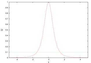
Figure 5: Effective potential $1/(1+\tau^{2})^{2}$ and effective energy $K_{z}^{2}=0.1$ for the solution of Schrödinger equation depicted at Fig. 4 .

For small enough effective energies $K_{z}^{2}$ we have a classical forbidden region where the magnetosonic waves are amplified.

This equation has two linearly independent solutions even (g) and odd (u)

$$\psi_{\mathrm{g}}(0) = 1,\quad\mathrm{d}_{\tau}\psi_{\mathrm{g}}(0)=0,$$ (228)

$$\psi_{\mathrm{u}}(0) = 0,\quad\mathrm{d}_{\tau}\psi_{\mathrm{u}}(0)=1,$$ (229)

Figure 6: Even wave eigenfunction: $\psi_{\mathrm{g}}(0)=1,$ $\mathrm{d}_{\tau}\psi_{\mathrm{g}}(0)=0.$

Figure 7: Odd wave eigenfunction: $\psi_{\mathrm{u}}(0)=0,$ $\mathrm{d}_{\tau}\psi_{\mathrm{u}}(0)=1$.

$$\psi_{\mathrm{g}}\!=\sqrt{1+\tau^{2}}\mathrm{H_{c}}(0,-\frac{1}{2},0,-\frac{K_{z}^{2}}{4},\frac{1+K_{z}^{2}}{4};-\tau^{2}),$$ (230)

$$\psi_{\mathrm{u}}\!=\tau\sqrt{1+\tau^{2}}\mathrm{H_{c}}(0,+\frac{1}{2},0,-\frac{K_{z}^{2}}{4},\frac{1+K_{z}^{2}}{4};-\tau^{2}),$$ (231)

and the general solution we will represent by the linear combination

$$\psi(\tau)=C_{\mathrm{g}}\psi_{\mathrm{g}}(\tau)+C_{\mathrm{u}}\psi_{\mathrm{u}}(\tau).$$ (232)

The confluent Heun function $\mathrm{H_{c}}(z)$ obeys the differential equation

$$y^{\prime\prime}+\left(4p+\frac{\gamma}{z}+\frac{\delta}{z-1}\right)y^{\prime}+\frac{4p\alpha z-\sigma}{z(z-1)}y=0,$$ (233)

with initial conditions

$$y(0)=0,\qquad y^{\prime}(0)=\frac{\sigma}{\gamma}$$ (234)

and close to $z=0$ has the Taylor expansion

$$\mathrm{H_{c}}(p,\alpha,\gamma,\delta,\sigma;z)=\sum_{n=0}^{\infty}C_{n}z^{n},$$ (235)

where for the coefficients we have the initial conditions $C_{-1}=0$ and $C_{0}=1$ and recursion

$$C_{n+1}=-(g_{n}C_{n}+h_{n}C_{n-1})/f_{n},\quad n=0,1,2,\dots$$ (236)

where

$$g_{n} = n(n-4p+\gamma+\delta-1)-\sigma,$$ (237)

$$h_{n} = 4p(n+\alpha-1),$$ (238)

$$f_{n} = -(n+1)(n+\gamma).$$ (239)

For large enough arguments we have the expansion

$$\mathrm{H_{c}}(p,\alpha,\gamma,\delta,\sigma;z)=\sum_{n=0}^{\infty}C_{n}^{(\infty)}z^{\alpha-n},$$ (240)

where only the recursion functions are different

$$g_{n}^{(\infty)} = (\alpha+n)(n-4p-\gamma-\delta+1)-\sigma,$$ (241)

$$h_{n}^{(\infty)} = -(\alpha+n-1)(\alpha+n-\gamma),$$ (242)

$$f_{n}^{(\infty)} = -4p(n+1).$$ (243)

F.3 Simple quantum mechanical problem

In order better to analyze the effective MHD equation Eq. (227) we will solve the corresponding quantum mechanical problem when we have tunneling trough the barrier $2m\tilde{U}/\hbar^{2}=1/(1+\tau^{2})^{2},$ supposing that $\psi$ is a complex function. We have falling wave with unit amplitude, reflected wave with amplitude $R$ and transmitted wave with amplitude $T$

$$\psi(\tau\rightarrow-\infty) \approx \exp(iK_{z}\tau)+R\exp(-iK_{z}\tau),$$ (244)

$$\psi(\tau\rightarrow+\infty) \approx T\exp(+iK_{z}\tau).$$ (245)

Using the asymptotic of the eigenfunctions

$$\psi_{g}\approx\left\{\begin{array}[]{l}D_{\mathrm{g}}\cos(K_{z}\tau-\phi_{\mathrm{g}}),\quad\mbox{for }\tau\rightarrow-\infty,\\ D_{\mathrm{g}}\cos(K_{z}\tau+\phi_{\mathrm{g}}),\quad\mbox{for }\tau\rightarrow+\infty,\end{array}\right.$$ (246)

$$\psi_{u}\approx\left\{\begin{array}[]{l}-D_{\mathrm{u}}\cos(K_{z}\tau-\phi_{\mathrm{u}}),\quad\mbox{for }\tau\rightarrow-\infty,\\ \;\;\,D_{\mathrm{u}}\cos(K_{z}\tau+\phi_{\mathrm{u}}),\quad\mbox{for }\tau\rightarrow+\infty\end{array}\right.$$ (247)

and solving the matrix problem we obtain

$$C_{\mathrm{g}}^{\mathrm{(q)}}D_{\mathrm{g}}=\exp(i\phi_{\mathrm{g}}),\qquad C_{\mathrm{u}}^{\mathrm{(q)}}D_{\mathrm{u}}=-\exp(i\phi_{\mathrm{u}})$$ (248)

Then for the tunneling coefficient we derive

$$\mathcal{D}=|T|^{2}=\mathrm{s_{ug}^{2}},\qquad\mathrm{s_{ug}}=\sin(\phi_{\mathrm{u}}-\phi_{\mathrm{g}})$$ (249)

Figure 8: Coefficient of transmission through quantum barrier as function of wave-vector $D=\cos^{2}\Theta_{ug}$. This coefficient parameterized amplification of alfvons $A=2/D-1$.

Let us introduct notation

$$\varphi_{u}=\phi_{u}+\frac{\pi}{2},$$ (250)

then $\Theta_{gu}=\phi_{g}-\varphi_{u}$.

F.4 MHD and real $\psi$

For the considered MHD problem $\psi$ is a real variable with asymptotic

$$\psi\approx\left\{\begin{array}[]{l}\quad\;\cos(K_{z}\tau-\phi_{\mathrm{i}}),\quad\mbox{for }\tau\rightarrow-\infty,\\ D_{\mathrm{f}}\cos(K_{z}\tau+\phi_{\mathrm{f}}),\quad\mbox{for }\tau\rightarrow+\infty.\end{array}\right.$$ (251)

Solving analogous 2$\times$2 matrix problem we derive

$$C_{\mathrm{g}}^{\mathrm{(c)}}D_{\mathrm{g}}=\mathrm{\frac{s_{iu}}{s_{gu}}},\qquad C_{\mathrm{g}}^{\mathrm{(c)}}D_{\mathrm{u}}=\mathrm{\frac{s_{ig}}{s_{gu}}}$$ (252)

and for the phase and amplification of the signal we have

$$\tan\phi_{\mathrm{f}}=\mathrm{\frac{s_{ig}s_{u}+s_{iu}s_{g}}{s_{ig}c_{u}+s_{iu}c_{g}}},$$ (253)

$$\mathcal{A}(\phi_{\mathrm{i}},K_{z}^{2})=D_{\mathrm{f}}^{2}=\frac{\mathcal{N}}{\mathcal{D}},$$ (254)

$$\mathcal{N}=\mathrm{(s_{ig}s_{u}+s_{iu}s_{g})^{2}+(s_{ig}c_{u}+s_{iu}c_{g})^{2}},$$ (255)

where

$$\mathrm{s_{ig}} = \sin(\phi_{\mathrm{i}}-\phi_{\mathrm{g}}),\quad\mathrm{s_{iu}}=\sin(\phi_{\mathrm{i}}-\phi_{\mathrm{u}}),$$ (256)

$$\mathrm{s_{g}} = \sin(\phi_{\mathrm{g}}),\quad\mathrm{s_{u}}=\sin(\phi_{\mathrm{u}}),$$ (257)

$$\mathrm{c_{g}} = \cos(\phi_{\mathrm{g}}),\quad\mathrm{c_{u}}=\cos(\phi_{\mathrm{u}}).$$ (258)

For large enough wave-vectors we have the asymptotic

$$\phi_{\mathrm{g}}(K_{z}^{2}\gg 1)=0,\qquad\phi_{\mathrm{u}}(K_{z}^{2}\gg 1)=-\frac{\pi}{2}.$$ (259)

Figure 9: Numerical solution of Schrödinger equation for amplitude of Alfvén waves. Property function is approximation by two sinusoid connected with cusp corresponding of $\delta$-like potential in relevant quantum mechanical problem. Initial conditions are: $K_{z}=0.05$ $\psi(\tau=-1000)=\cos(K_{z}\tau-\varphi_{0})$ ; $\mathrm{d}_{\tau}\psi(\tau=-1000)=-K_{z}\sin(K_{z}\tau-\varphi_{0}),$ and $\varphi_{0}=\frac{\pi}{2}.$

Figure 10: Numerical solution of effective Schrödinger equation illustrated amplification of amplitude for small values of wave-vector. Initial conditions are: $K_{z}=0.05$ $\psi(\tau=-1000)=\cos(K_{z}\tau-\varphi_{0})$ ; $\mathrm{d}_{\tau}\psi(\tau=-1000)=-K_{z}\sin(K_{z}\tau-\varphi_{0}),$ and $\varphi_{0}=\pi.$

Figure 11: Phase analysis of wave equation:the phases of odd $\phi_{\mathrm{u}}$ and even $\phi_{\mathrm{g}}$ function of Schrödinger equation. Phase difference $\Theta_{gu}=\phi_{g}-\varphi_{u}$ parameterized reflection coefficient of quantum mechanical problem and amplification coefficient of MHD problem.

Figure 12: Continuous curve above is phase of odd wave function $\phi_{\mathrm{u}}$, dots curve under is phase of even wave function $\phi_{\mathrm{g}}$ shifted by $\frac{\pi}{2}.$

F.5 Random phase approximation statistical problem

Finally simple angle averaging

$$\int_{-\pi}^{\pi}\frac{\mathrm{d}\phi_{\mathrm{i}}}{\pi}\mathcal{N}(\phi_{\mathrm{i}})=2-\mathrm{s_{\mathrm{ug}}^{2}}=2-\mathcal{D}$$ (260)

gives

$$\mathcal{A}(K_{z}^{2})=\frac{2}{\mathcal{D}}-1=\frac{2}{\mathrm{s_{ug}^{2}}}-1.$$ (261)

In such a way we analyzed the relation between quantum mechanical treatment and MHD one for the effective Schrödinger equation.

F.5.1 Longwavelength approximation

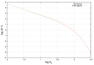
Figure 13: Amplification of Alfvén waves keystone of the theory of heating of accretion disks; amplification in Bell as function of logarithm of the dimensionless wave-vector; 1 Bell means 10 times energy amplification. The dotted line is the $\delta$-like long wavelength approximation which is adequate when the amplification is significant $\mathcal{A}\gg 1.$ This exact solution at $K_{y}=0$ is a test for Monte Carlo calculations in the general case.

For small wave-vectors $K_{z}^{2}\ll 1$ we have $\delta$-potential approximation in the effective Schrödinger equation Eq. (227)

$$\frac{1}{(1+\tau^{2})^{2}}\rightarrow\lambda\delta(\tau),\quad\lambda\equiv\int_{-\infty}^{+\infty}\frac{\mathrm{d}\tau}{(1+\tau^{2})^{2}}=\frac{\pi}{2}.$$ (262)

The substitution of $\lambda\rightarrow 2\lambda$ gives exactMishonov:09 result at long-wavelength limit. The wave function is continuous at $\tau=0$ i.e.

$$\psi(-0)=\psi(+0),$$ (263)

but the first derivative have a jump which can be calculated integrating Eq. (227) in a small vicinity of $\tau=0$

$$\mathrm{d}_{\tau}\psi(+0)-\mathrm{d}_{\tau}\psi(-0)=\lambda\psi(0),$$ (264)

we use obvious alleviation of the notations. For the wave function

$$\psi(\tau<0)=\cos(K_{z}\tau-\phi_{i}),\quad\psi(\tau>0)=D_{f}\cos(K_{z}\tau+\phi_{f})$$ (265)

one can easily solve the equations Eq. (263) and Eq. (264) which gives

$$D_{\mathrm{f}}=\sqrt{1+\frac{\lambda}{K_{z}}\cos(2\phi)+\frac{\lambda^{2}}{K_{z}^{2}}\cos^{2}(\phi)},$$ (266)

$$\phi_{\mathrm{f}}=\arccos(\frac{\cos\phi_{\mathrm{i}}}{D_{\mathrm{f}}}).$$ (267)

The averaging of the amplification coefficient with respect of the initial phase gives

$$\mathcal{A}=\int_{0}^{\pi}D_{\mathrm{f}}^{2}\frac{\mathrm{d}\phi_{\mathrm{i}}}{\pi}=1+\frac{\lambda^{2}}{2K_{z}^{2}}\approx\frac{\pi^{2}}{8K_{z}^{2}}=\frac{1}{8}\left(\frac{\pi A}{k_{z}V_{A}}\right)^{2}\gg 1.$$ (268)

In other words the Alfvén waves amplification can be significant for the long waves. For the eigenfunctions in this approximation we have

$$\psi_{\mathrm{g}} \approx -\frac{1}{\gamma_{\mathrm{g}}}\sin(K_{z}|\tau|-\gamma_{\mathrm{g}}),\quad K_{z}>0,$$ (269)

$$\gamma_{\mathrm{g}} = \frac{2K_{z}}{\lambda}=\frac{4K_{z}}{\pi}\ll 1,$$ (270)

$$\phi_{\mathrm{g}} = \frac{\pi}{2}-\gamma_{\mathrm{g}}=\frac{\pi}{2}-\frac{4K_{z}}{\pi},$$ (271)

$$\psi_{\mathrm{u}} \approx \frac{1}{K_{z}}\sin(K_{z}\tau),$$ (272)

$$\phi_{\mathrm{u}} \approx -\frac{\pi}{2}\quad\phi_{\mathrm{ug}}=\gamma_{\mathrm{g}}-\pi,$$ (273)

$$\mathrm{s_{gu}} \equiv \sin(\phi_{\mathrm{g}}-\phi_{\mathrm{u}})\approx\gamma_{\mathrm{g}}=\frac{4K_{z}}{\pi}.$$ (274)

The substitution of this approximate formula for $\mathrm{s_{gu}}$ in the general formula for the amplification Eq. (261) reproduces the long wavelength result Eq. (268).