The Vimos VLT Deep Survey: Compact structures in the CDFS

We have used the Vimos VLT Deep Survey in combination with other spectroscopic, photometric and X-ray surveys from literature to detect several galaxy structures in the Chandra Deep Field South (CDFS). Both a friend-of-friend based algorithm applied to the spectroscopic redshift catalog and an adaptative kernel galaxy density and colour maps correlated with photometric redshift estimates have been used.

We mainly detect a chain-like structure at z=0.66 and two massive groups at z=0.735 and 1.098 showing signs of ongoing collapse. We also detect two galaxy walls at z=0.66 and at z=0.735 (extremely compact in redshift space). The first one contains the chain-like structure and the last one contains in its center one of the two massive groups. Finally, other galaxy structures that are probably loose low mass groups are detected.

We compare the group galaxy population with simulations in order to assess the richness of these structures and we study their galaxy morphological contents. The higher redshift structures appear to probably have lower velocity dispersion than the nearby ones. The number of moderatly massive structures we detect is consistent with what is expected for an LCDM model, but a larger sample is required to put significant cosmological constraints.

1 Introduction

Modern galaxy surveys usually map the large scale structure of the Universe over large contiguous regions at low redshifts (e.g. Folkes et al. 1999 for the 2dF survey or Castander 1998 for the SDSS) or more sparsely up to z$\sim$1. These surveys use for example clusters of galaxies (e.g. Romer et al. 2001) or larger scale filaments and walls (e.g. Davé et al. 1997) to constrain cosmological models. However, it is very rare to be able to combine multi-wavelength data over relatively large contiguous regions in order to search homogeneously for structures up to z$\sim$1. Similarly, spectroscopic samples are usually very incomplete inducing several detection biases.

In this framework, the CDFS area has become these last years an intensively surveyed area in several wavelengths: from X-rays (e.g. Giacconi et al. 2002) to optical and near infrared (e.g. Moy et al. 2003, Arnouts et al. 2001), both in imaging and spectroscopic modes (e.g. Gilli et al. 2003, Le Fèvre et al. 2004). Recently, a very large catalog of 1599 spectra was released by the VVDS team (Le Fèvre et al. 2004). These new redshifts were measured in an area of 21’$\times$21.6’ and include a total of 1452 galaxies, 139 stars and 8 QSOs. The redshift distribution is peaked at a median redshift of 0.73 and include measurement down I_AB=24. Combination of these data makes now possible galaxy structure identifications in this field with a five times larger spectroscopic data sample as the one used for example in Gilli et al. (2003). In a companion paper (Scaramella et al. 2006) very large scale and diffuse galaxy structure will be presented while we concentrated on compact structures (groups, clusters and compact walls) in this paper.

Detecting groups or clusters is not, however, an easy task, essentially because these are not well defined objects but assemblies of objects. Even if they can best be defined as ”potential wells”, which are responsible for lensing effect and X-ray emission of the hot gas, the use of these techniques requires, especially for distant systems, complementary photometric and spectroscopic observations of the candidate member galaxies in order to measure their redshift and colors.

Historically (e.g. Abell 1989 and references therein), clusters or groups appear as excess in the galaxy density field but the use of the ”number density excess” with respect to the background as a method of detection becomes rapidly inefficient as soon as more distant systems are searched. Indeed, the contrast is decreasing as long as the apparent limiting magnitude is increasing. This difficulty is still present when using the third dimension (in terms of redshift) since, even if virialized structures extend on more or less six times their velocity dispersion in redshift space, any survey probes less and less clusters member galaxies in apparent magnitude limited surveys.

We present our results based on public spectroscopic redshifts, Combo17 photometric data (e.g. Wolf et al. 2004) and X-ray source catalogs (Giacconi et al. 2002). In this paper, we combine these data with our own spectroscopic observations of the CDFS field (Le Fèvre et al. 2004) available at the CENCOS database (http://cencosw.oamp.fr/FR/index.fr.html). The methods developed in this paper will be used to search and study clusters in larger samples such as the complete Virmos VLT Deep Survey (VVDS hereafter).

Section 2 presents the detection methods and the samples we used. Section 3 presents the structure analysis methods. Sections 4 reviews the galaxy structures we detected. The final discussion of our results is in Section 5. All quantities were calculated assuming a standard flat LCDM model with H₀=65 km/s/Mpc, $\Omega_{m}$=0.3, $\Omega_{\Lambda}$=0.7.

Figure 1: Galaxy redshift sampling rate for I magnitudes between 17 and 24 in the CDFS. Completeness is given in percentage on the vertical axis.

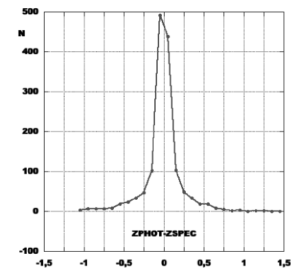
Figure 2: Histogram of the difference between spectroscopic and photometric redshifts in the CDFS using Combo17 magnitudes down to I=24.

Figure 3: Upper figure: 3D view of the spectroscopic catalog distribution. Lower figure: 3D view of the photometric redshift catalog distribution. The thin z=0.73 wall is visible in the upper figure and merged with the z=0.66 large structure in the lower figure.

Figure 4: Gap redshift histogram in the CDFS spectroscopic survey.

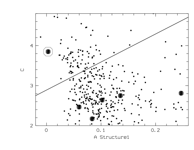
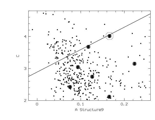
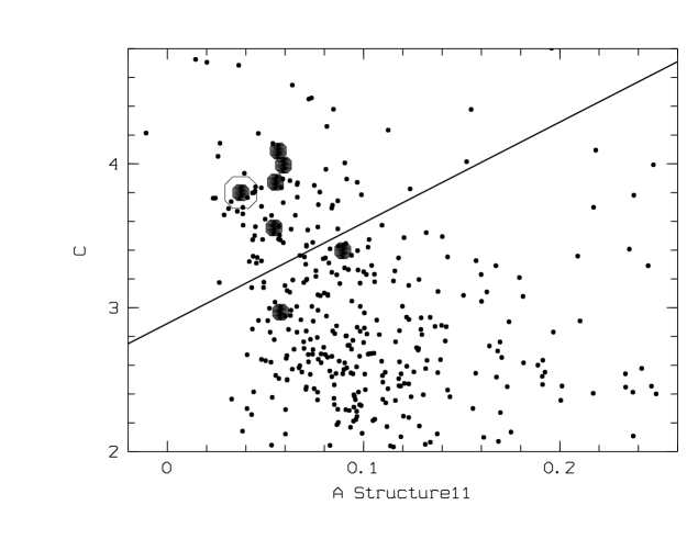
Figure 5: Asymmetry versus Concentration of galaxies in Structures 1, 9 and 11. The solid line symbolizes the separation between early and late morphological types. Filled circles are the galaxies inside the considered structure, circled filled circle is the brightest galaxy of the structure and dots are all the field galaxies along the CDFS line of sight.

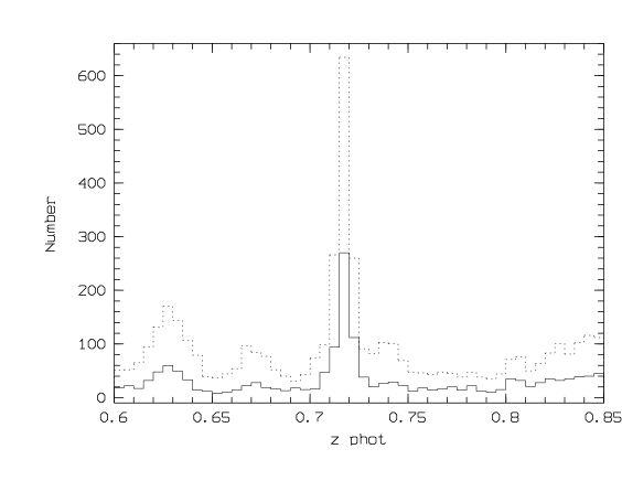
Figure 6: Histograms of photometric redshifts around the z=0.73 wall. Dashed line: inside the spectroscopic area, solid line: outside the spectroscopic area and inside the photometric redshift area.

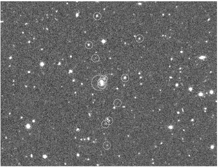
Figure 7: HST I image of Structure 11-1 at z=0.73 with galaxies associated to the structure (small circles) and the X-ray source (large circle). Size of the image is 5.1’$\times$3.4’.

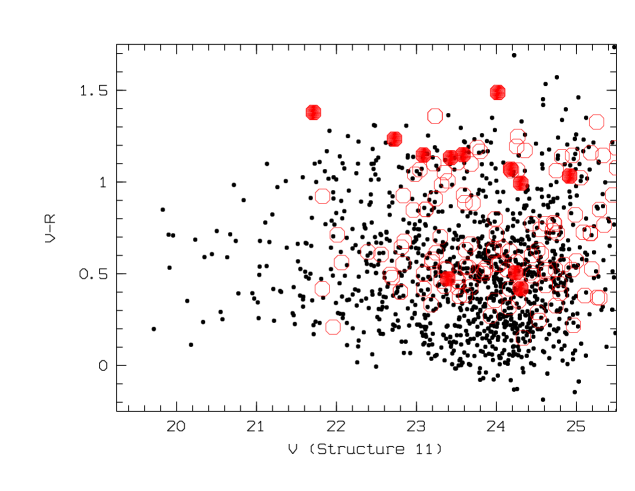
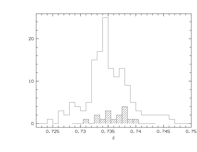
Figure 8: Top: color Magnitude Relation (CMR) for Structure 11. X-axes are the V magnitudes and y-axes are the V-R colors. Dots are field galaxies with measured spectroscopic redshift. Structure 11 (the z=0.735 wall) is shown as open circles while the central group (Structure 11-1) is shown as filled circles. Bottom: redshift histogram with a step of 300 km/s (dashed histogram is the structure 11-1).

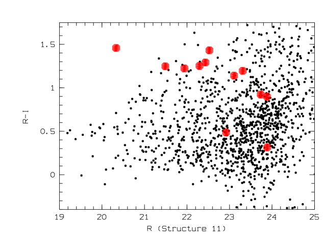
Figure 9: Same as Fig. 8 with R/R-I CMR and for Structure 11.

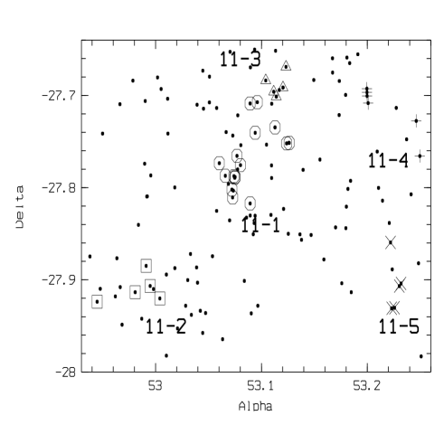
Figure 10: Dots: from spectroscopy, all galaxies inside the z$\sim$0.735 wall (Structure 11). Circled dots: main dynamical group. Squares, triangles and crosses: additionnal dynamically linked groups.

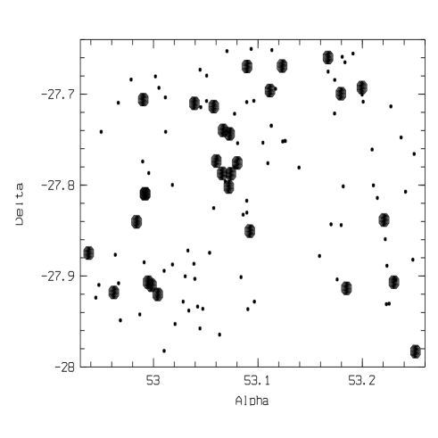
Figure 11: Dots: all galaxies inside the z$\sim$0.735 wall (Structure 11). Filled circles: early type galaxies from morphological classification.

Figure 12: Adaptative kernel density contours of the z=0.735 wall from photometric redshifts. East is to the right and north is to the top. Top: galaxies with B-R=[1.5;2] are overplotted. Middle: galaxies with B-R greater than 2 are overplotted. Bottom: 2D spectroscopic redshift sampling rate: the darker the color code, the higher the sampling rate, the lighter the color code, the lower the sampling rate. The sampling rate is typically varying from 15 to 30$\%$.

2 Detection methods and structure galaxy sample

2.1 What we are looking for: aims and strategy

We present here several key numbers. A galaxy structure appears on the sky (counted in 2D) as an excess in the galaxy density field. For a given limiting magnitude, this contrast is decreasing with redshift. Table 1 shows for example this contrast for a Coma-like cluster put at z=0.5 and 1 for several limiting apparent magnitudes (assuming no evolution).

However, assuming that the red sequence (corresponding to early type objects) is present at least in the rich structures, its detection in photometric bands matching the expected redshift either using color magnitude relation or color density maps (as described below) is a potentially adequate method.

Contrarily to photometric catalogs that provide almost uniform coverage on broad regions of the sky, uniform spectroscopic coverage (and especially of dense areas as groups or clusters) even with the most efficient instrumentation needs a considerable effort to ensure a sufficient sampling both in terms of space and magnitude range. Consequently, the characteristics of the detected structures clearly suffer from the bias induced by observational procedures. The VVDS aims to overcome these difficulties by using an optimal strategy in terms of spatial coverage and redshift sampling (e.g. Le Fèvre et al. 2004). The resulting effects on the detection of structures have already been discussed in Rizzo et al. (2004).

2.2 The spectroscopic sample

In order to search for compact structures inside the Chandra Deep Field South we used all the available redshifts in the literature in this region.

Starting from a VVDS catalog of 1460 redshifts with quality flags greater than 1 (i.e. greater than 75$\%$ confidence level, see Le Fèvre et al. 2004) and using an identification distance of 1”, we added 129 additionnal redshifts from the ESO-GOODS sample using spectra with quality strictly greater than 0.5, 222 redshifts from Szokoly et al. (2004) measured on spectra with qualities equal to A and B and 7 redshifts from the 2dF survey. In total, we are therefore using a catalog of 1818 redshifts. This represents about 25$\%$ of all galaxies in the CDFS field of view down to I=24. As demonstrated in Scaramella et al. (2006), these catalogs are in very good agreement regarding redshift estimates and merging them is, therefore, not a concern.

As a first step, we limited this catalog to redshift greater than 0.16 as it was very unlikely to detect interesting large scale features at lower redshift due to our small angular extent ($\sim$18’$\times$19’). Moreover, there is an Abell cluster (A3141) at z$\sim$0.11 only at 69’ from the CDFS field center and the infalling field galaxies onto this cluster are probaly significantly populating the CDFS area. The final catalog contains 1591 redshifts greater than 0.16. The result of such a building process is that the sampling rate of the galaxy redshift catalog is quite inhomogeneous across the field of view (Fig. 1) because all the surveys we used are not covering the same area and have different sampling rates. VVDS data are quite homogeneous over a large field while other surveys are uniform only over smaller areas. However, as we are searching for distant structures, the more galaxy redshifts we have, the more efficient is their detection.

As discussed above, even using redshifts, detection of distant structures (for which m^∗ is close to the survey limiting magnitude) is not easy. Disentangling structure members from field galaxies and estimating the velocity dispersion requires uncertainties on velocities to be well estimated. Here we took advantage of having galaxies measured at least twice to have such a realistic estimate. Using the 187 galaxies observed two times and with a 75$\%$ confidence redshift estimate from both observations, it turns out that we have a dispersion close to 0.002, not strongly dependent on magnitude nor redshift up to z$\sim$1.2. We adopted this value as the spectroscopic redshift uncertainty for all galaxies. Uncertainties listed in Table 4 and 5 take into account this value.

We note that the K20 data (e.g. Cimatti et al. 2002) were not public at the time of the present work completion. We plan however to use these data to search for very distant structures in the CDFS in a future article.

2.3 The photometric samples

We used the Combo-17 magnitude catalog (e.g. Wolf et al. 2004). This catalog provides 17 photometric bands. We limited ourselves to I=24 which is the spectroscopic magnitude limit. Using the Combo-17 photometry, photometric redshifts have been calculated and compared to spectroscopic redshifts using the code ”LePhare” (http://www.lam.oamp.fr/arnouts/LE-PHARE.html). When limiting the samples to z_spec=1.2, it turns out (see Fig 2) that in about 75$\%$ of cases, the difference is less than 0.15. Moreover, we used all spectroscopic spectra with a confidence level greater than 75$\%$. This means that we are not exempt from spectroscopic errors in redshift estimates, increasing artificially this difference of less than 0.15.

Using the spectroscopic sample and the Combo17 magnitudes, we were also able to compute a ”photometric” type (see Section 3.3.2). Both photometric redshift and photometric type estimates are distinct from the ones performed by the Combo17 team and will be described in a future paper.

As the spatial coverage of photometric data is uniform, we take advantage of the good quality of photometric redshifts to complement our spectroscopic analysis by performing density and color maps within photometric redshift slices (see next section). Structures detected with several methods (spectroscopic AND photometric) have a better chance to be real. However, due to uncertainties of photometric redshifts, real structures will be both broadened and contaminated by adjacent photometric redshift slices. Advantages (sharpness) and disadvantages (sparse sampling) of spectroscopic redshifts versus advantages (good sampling) and disadvantages (broadening) of photometric redshifts are illustrated in Fig 3 where the 3D distribution of galaxies is plotted using spectroscopic and photometric redshifts. In both cases, the main large scale structures are visible (see following discussions).

2.4 The spectroscopic structure detection method

The method we used to detect stuctures is a friend of friend based algorithm described in Adami $\&$ Mazure (2002) and Rizzo et al. (2004). This algorithm first makes a classical count-in-cells of the galaxies in the redshift catalog (using a tunable window size on the sky and in the redshift space). The cell size projected on the sky is chosen according to the type of structures searched for (for clusters of galaxies, it corresponds to the characteristic size of such structures at a given redshift: we adopted a value of 1Mpc). The size in redshift space is also characteristic of the structures but can also be infered from the redshift difference between the closest galaxy pairs in the sample (see Fig 4). The peak of galaxies below a given redshift separation gives a statistical definition of the typical size of structures. For the present case, we used 0.0026 (the value after which the distribution in Fig 4 becomes more or less constant). We note that this value is probably affected by the non-homogeneous redshift sampling rate across the field of view. If the number of galaxies in a given cell is large enough, this cell is kept as significantly populated. Then, a percolation algorithm is associating individual adjacent cells in larger structures. We chose in our analysis parameters adapted to the detection of compact structures. The parameters used are similar to the ones given in Rizzo et al. (2004). The maximum redshift extension of a structure was fixed to $\Delta z=0.02$. Elementary structures were merged when closer than 2Mpc. The minimum number of galaxies per elementary structure was set to 4 and the minimum number of galaxies per percolated structure (final structure) was set to 5. The size of the individual cells (where elementary structures were searched) was fixed to 2 Mpc, which was converted to the corresponding angular size as a function of redshift; the search was done in different redshift slices: [0.16,0.31], [0.31,0.40], then between z=0.40 and z=1.70 in slices of width $\Delta z=0.10$. We also checked separations between each slices, detecting for example in this way S15 (z=1.098).

The physical parameter that will limit the completeness of the structure catalog is the completeness of the redshift catalog. For a constant galaxy sampling in terms of redshift measures, we will for example more easily detect the richest structures because these will be sampled with more redshifts. The velocity dispersion is not by itself, however, a limiting parameter (besides the fact that poor structures have generally low velocity dispersions). We fixed the minimal number of galaxies with a redshift inside a structure to 5 (i.e. structures with 4 galaxies or less are automatically excluded as considered as spurious detections).

We do not attempt to precisely estimate the structure detection rate in this paper because of the complex galaxy redshift catalog sampling rate. However, following Rizzo et al. (2004), the structure detection rate should be lower than 70$\%$ at z=0.3, lower than 50$\%$ at z=0.6 and about 10$\%$ for z greater than 1. We remark, as well, that nearly all structures detected with this method are probably real with only about 10$\%$ expected to be spurious (Rizzo et al. 2004), independently of the structure apparent richness.

We note that a by-product of this structure detection procedure is a field galaxy redshift catalog, i.e. the catalog of galaxies not included in any compact structures.

2.5 The photometric structure detection method

While the previous method allows to disantangle close structures along the line of sight thanks to the precision of the spectroscopic redshifts, this method is limited by the completeness level of the spectroscopic sample. Low sampling regions will not provide, therefore, a good structure detection rate. In order to solve this problem, we used a second method based on photometric redshift estimate and adaptative kernel color and galaxy density maps.

Adaptative kernel galaxy density maps are a common way to detect and study nearby galaxy structures (e.g. Adami et al. 1998(a)). We estimated a significance level for these maps using a bootstrap technique (e.g. Biviano et al. 1996) with 1000 resamplings. This method is very efficient as long as the detectable cluster galaxy population is dominating the detectable field galaxy population. When trying to detect distant structures, however, the cluster/field galaxy ratio becomes very low and structures becomes virtually undetectable. In order to increase this ratio, we used the photometric redshift estimates. We proceed in two steps:

-First, we divide the galaxy catalog into slices of $\pm$0.1. Such a width is similar to the depth of nearby galaxy catalogs used to search for nearby structures (e.g. Adami et al. 1998(a)) and is larger than the mean photometric redshift uncertainty for individual galaxies.

-Second, we use the classical adaptative kernel galaxy density map method to eyeball the galaxy overdensities in the given redshift bin.

This method is applied to a complete photometric redshift catalog, so we are not affected by inhomogeneous sampling rate. However, our photometric redshift estimate is less precise than the spectroscopic estimate (even if one of the most precise ever computed: see Fig 2), and this, therefore, induces a smoothing of the redshift distribution and reduces the ability to disantangle close structures along the line of sight. We show in Fig. 3 the distribution along the CDFS line of sight of the spectroscopic and photometric redshifts to illustrate this problem. Similar structures are visible in both catalogs, but photometric redshift distribution is less precise. The z=0.66 and z=0.735 walls are for example almost merged in a single structure using photometric redshifts only, while we create fake concentrations around z=0.87.

2.6 Color spatial distribution

As discussed above, rich clusters are generally characterized by an excess of red objects even to z$\sim$1. The colors of elliptical galaxies are given in Table 2 for several redshifts (magnitude bands are chosen to encompass the 4000$\AA$ break given the redshift). As a generalisation of the previous method, we also used the mean color maps in the $\pm$0.1 photometric redshift slices using the color corresponding to the mean redshift. Computed with the adaptative kernel method, this allows us to locate immediately the early type galaxy concentrations in the redshift slices (assuming that red objects are preferentially early type objects) and to compare with simple galaxy overdensities. It also allows us to compare candidate structure locations with the location of the structures detected with the spectroscopic method.

3 Structure analysis methods

3.1 Galaxy velocity dispersion and spatial extension of the detected structures

For each of the detected structures, we computed the mean redshift, the cosmological velocity dispersion (with Biweight estimators from Beers et al. 1990) and the uncertainty on this value (using ROSTAT package with 1000 bootstraps, Beers et al. 1990). This uncertainty is a 1-$\sigma$ error. We also computed the spatial extension (computed as the maximum of the alpha and delta distribution second momentum) and the mean coordinates. All these values are given in Tables 4 and 5. We note that even using robust estimators, we gave confidence to the velocity dispersion estimate only when using more than 10 redshifts (e.g. Lax 1985).

3.2 Red sequences in Color Magnitude Relations (CMR)

Since the works of Baum (1959) and Sandage (1972) showing a correlation between galaxy type, magnitude and color for early type galaxies in clusters, the CMR is commonly used to characterize the cluster galaxy populations. Relatively old and virialized clusters have an old elliptical population and, therefore, exhibit a red sequence in the CMR (at least at low and moderate redshifts).

We apply the same test here with different magnitudes. Low redshift structures will be studied using the B and V magnitudes (Wolf et al. 2004), intermediate redshift structures with the V and R magnitudes and high redshift structures with the R and I magnitudes. These filter-pairs are chosen in order to encompass the 4000$\AA$ break according to the structure redshift. We used the Combo17 magnitudes because this is the only homogeneous and unbiased photometric sample from B to I in our whole field of view. Examples of expected values are given in Table 2.

We note that a large part of the structure sample has not a very early galaxy content. This makes impossible to define properly a red sequence and, therefore, to compute homegeneously for the whole sample a slope and a compactness. However, a possible test is to compare, using a 2D Kolmogorov Smirnov test, the structure galaxy distribution in the magnitude/color diagram with the field galaxy distribution in the same space. This test will give the percentage of representativity of the structure galaxy distribution compared to the field galaxy distribution. The higher the percentage, the more different the two distributions (value KS1 in Tables 4 and 5). We note that this test can be affected by inhomegeneous galaxy sampling, inducing observational statistical differences between the whole and the structure population.

3.3 Structure galaxy content

The galaxy content of the structures we detected is very important to estimate because it allows us to understand how the galaxy structures are evolving with redshift, mass and environment and how old these are. The key question is here to estimate the galaxy type. We have used three independent methods detailed in the following.

3.3.1 Spectral characteristics

First, we used the presence of emission or absorption lines in galaxy spectra, given that pure emission line galaxies are preferentially late type galaxies and that pure absorption line galaxies are preferentially early type galaxies (see e.g. Biviano et al. 2002).

Using the VVDS spectra only (most of our sample), we were, therefore, able to distinguish between galaxies with emission lines, absorption lines or both (between z=0.2 and z=1.15: the redshift range where we detected structures with VVDS data only). Then, we computed the percentage of pure emission and absorption line galaxies in our catalog of structures. We kept only structures with more than 5 spectra and at least half of the structure population with a spectrum (as we have only access to the VVDS spectra).

However, the detectability of a given emission or absorption line is a complex interplay of several factors. Most of the time we are not able to follow a spectral line from z=0.2 to z=1.15 (due to our limited spectral range: $\sim$[5500A;9400A]). For distant (and faint) galaxies, emission lines are also usually easier to detect than absorption lines. A simple representation of the variation with redshift of the percentage of emission and absorption lines would, therefore, be biased. For example, for z$\geq$0.9 galaxies, the only major visible emission line is [OII]: this will artificially lower the number of emission line-detected galaxies. In order to remove these effects, we also computed the percentage of pure emission and absorption line galaxies in our catalog of field galaxies as a function of redshift. This allowed us to compare the structure galaxy content with the field galaxy content in order to determine if, for a given redshift, a structure galaxy content is morphologically earlier than the field population.

3.3.2 Photometric type

Second, we used rest frame colors computed using Combo17 magnitudes (Wolf et al. 2004 and see Ilbert et al. 2005). These colors computed in the AB system using B and I rest frame magnitudes are related to galaxy types according to Wolf et al. (2004). We divided these types into 2 bins: Elliptical + early spirals and late spirals + Irregulars. We used only structures with more than 5 galaxies with an estimated morphology.

3.3.3 Morphological type

Third, we used the classification made by Lauger et al. (2005) for galaxies in the ESO/GOODS CDFS area (Giavalisco et al. 2004). This method is based on asymmetry and concentration and a visual inspection of the galaxies from HST data in several bands (rest-framed in the B band). We only review here the salient points of this method:

- the classification was made using the F435W, F606W, F775W and F850LP HST filters in the B rest-frame passband

- the method is based on the Asymmetry (A) and light concentration (C) estimate (e.g. Bershady et al. 2000) calibrated in the (A,C) parameter space by eye-balled morphological types (using the same HST ACS data)

- the basic method is only able to discriminate between bulge dominated (assumed to be early type) and disk dominated (assumed to be late type) objects. We adopted the same discrimination as in Lauger et al. (2005) and Ilbert et al. (2005) (see also Fig. 5).

We finally computed (using a Kolmogorov-Smirnov 2D test) the probability of the A/C distributions of structure galaxies in Fig. 5 to be different from the field galaxy distribution in structures with more than 5 estimated morphological types (see KS2 values in Tables 4 and 5).

3.4 Richness estimate

When detecting a structure with the spectroscopic method, we produce a catalog of the galaxies which are within the structure. However, it is not trivial to discriminate between galaxies really belonging to this structure and just passing-through galaxies (at the same structure redshift but not physicaly bounded with the structure potential). This would require larger samples of redshifts (of the order of 50 redshifts per structure: e.g. Mazure et al. 1996). This is impossible with our data due to the high redshift of the detected structures combined with the magnitude limit, the relatively low sampling rate and the low-richness nature of the detected structures.

A possible resulting problem is the inclusion in the structures of non-member galaxies. This can artificially increase the structure richness if estimated with the number of included galaxies (we are simply including field galaxies inside the structure) or with the velocity dispersion (passing through galaxies should have high relative velocities, increasing the velocity dispersion estimate). We had therefore to find a way to compare the structure class (for a given redshift) estimated via the number of galaxies included or estimated via the velocity dispersion. The number of spectroscopically measured galaxies in a given structure depends on:

- the number of available targets down to the survey limiting magnitude (interplay between the structure richness, the survey limiting magnitude and the structure redshift)

- the galaxy sampling rate in the survey inside the structure region

Using simulated cones (Rizzo et al. 2004) with richness-, redshift- and position-controled included clusters, we were able, using the VVDS SSPOC tool (Bottini et al. 2005), to compute numbers of targeted galaxies down to I=24 theoretically present in our detected structures given their redshift, velocity dispersion and position in the field (that give the sampling rate). Results are shown in Table 3. This allowed us to determine for the most interesting structures if the populations we detected were reasonably rich.

4 Detected structures

4.1 The z$\sim$0.73 wall

When applying our spectroscopic structure detection algorithm, we tuned the parameters to detect compact cluster-like structures. We detected with these parameters a wall at z=0.735 already detected by Gilli et al. (2003), extending across the whole field of view covered with spectroscopic redshifts (about 9 Mpc), with a velocity dispersion as low as 665$\pm$116 km/s and sampled with 145 galaxies. This structure is as compact in redshift as a cluster of galaxies and as extended on the sky as a supercluster of galaxies. Such a structure could be also interpreted as a collapsing sphere of comoving radius of a few Mpc, producing a velocity dispersion close to the one observed. In order to check this point, we used the whole field of view with available photometric redshifts (not only spectroscopic redshifts). This field is 1.9 larger in alpha and 1.4 times larger in delta, covering about 15Mpc. Fig. 6 shows that the z=0.73 structure is still very significantly visible outside of the spectroscopic area. This leads to conclude that this structure is probably too large to be a simple collapsing sphere and is really a wall.

We note that using the Rostat package (Beers et al. 1990), we detect 9 significant empty redshift gaps inside the redshift distribution of the z=0.735 wall. This, added to the fact that there is no extended X-ray emission across the whole field of view and that there is no visible red sequence in the CMR (see Figs. 8 and 9), shows that this structure is not virialized. The galaxy velocity dispersion has, therefore, not to be taken as a measure of the mass of the system.

One region of the wall is particularly interesting as we clearly see the presence of a more compact object in the center (see Fig. 7). This structure is also an extended X-ray source (XID 566 in Giacconi et al. 2002).

In order to study more carefully the structure of the wall, we applied the Serna-Gerbal method (Serna $\&$ Gerbal 1996). This method allows the detection of substructures in galaxy clusters, estimating the link energy between galaxies of a compact structure. We detected 5 significant substructures inside Structure 11 (see Table 5). These structures appear both in galaxy density maps and galaxy color maps (for Structures 11-1, 11-2 and 11-4) computed using photometric redshifts.

The largest one is identified with the central group and associated with the extended X-ray source (XID 566). Sampled with 10 redshifts, this structure (Structure 11-1) has a velocity dispersion of 455$\pm$161 km/s. This is typical of a low mass cluster of galaxies (or a quite massive group). The Rostat package does not detect any significant empty redshift gap in the redshift distribution of the galaxies inside this structure. However, given the sampling rate at the place where this structure is detected and the redshift of this structure, we computed through simulations that such a $\sim$450km/s structure should be sampled with 20-30 objects. This is an indication that the velocity dispersion of structure 11-1 is probably overestimated. From the bolometric luminosity of 0.11 10⁴³ erg/s for this structure as computed from Giacconi et al. (2003) data, we can derive an independent estimate of the mass. Following for example Jones et al. (2003), this is typical of a normal group, with velocity dispersions around 200-300 km/s.

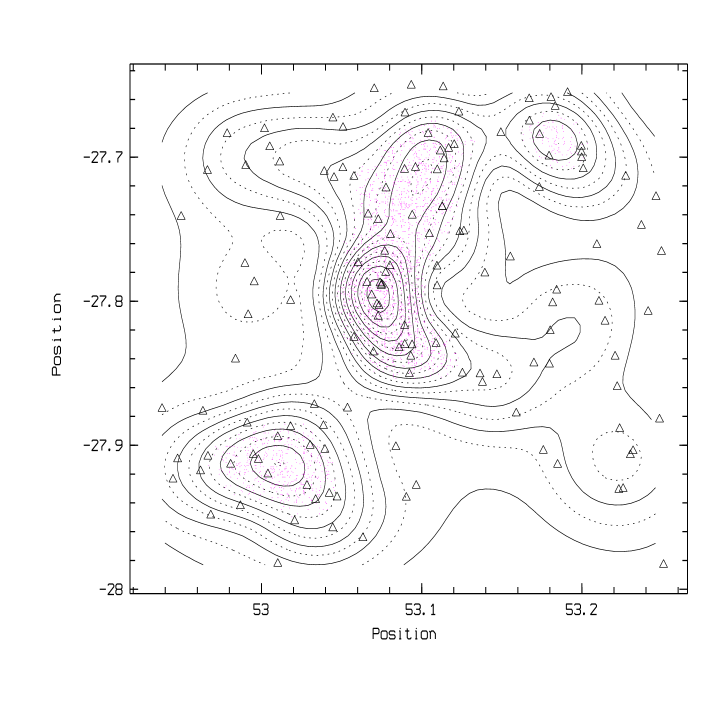
Figure 13: Isocontours of the galaxy (with a measured redshift) density across our CDFS field of view and inside the z=0.735 wall. Alpha and Delta coordinates are given. Triangles are the individual galaxies with a redshift inside the z=0.735 wall. Shaded areas are the areas where the galaxy density estimate is significant at the 3-$\sigma$ level.

The galaxy content of this structure is essentially made of early type galaxies from morphological estimates (see Fig. 5), very different from the field galaxy content, with a couple of central galaxies probably in a merging process (fig 13 of Giacconi et al. 2002). We used only these early type galaxies (from morphological estimates) in Figs. 8 and 9 to define the red sequence in the CMR.

The red sequence in the CMR is well defined for Structure 11-1 (see Figs. 8 and 9) and the galaxy distribution in the color/magnitude space is different from the field at the 99$\%$ level using both V/V-R and R/R-I. The red sequence for Structure 11-1 has also the correct position for z=0.735 (see Table 2).

All these arguments concur to show that we have detected a real low mass relatively old structure lying in the core of the z=0.735 wall.

The 4 other substructures (Structures 11-2, 11-3, 11-4 and 11-5) are sampled by 5 or 6 redshifts without extended X-ray counterparts. The corrected velocity dispersions of these structures ranges from 150 to 500 km/s but are typical of non virialized groups of galaxies given the abscence of X-ray emission (see Table 5). These groups appear in Fig.12 to be preferentially constituted of red (and probably early type) galaxies. This map has to be compared with Fig.11 showing early type galaxies from the morphological classification. At least for Structure 11-1, early type galaxies and red galaxies trace this same central structure. Other structures inside the wall are not very well traced by morphologicaly classified galaxy, but this is due to the fact that HST ACS data are not covering the corner edges of the CDFS field.

We computed an adaptative kernel 2D map of the z$\sim$0.735 wall galaxy density following the same recipe as described for example in Adami et al. (1998b) (see Fig.13) using first only galaxies with a measured redshift. Triangles are the galaxies. Shaded areas are the places where the galaxy density estimate is significant at the 3-$\sigma$ level (from 1000 bootstrap resamplings), i.e. where the galaxy overdensity is significant. This map is very similar to Fig.12 (on a slightly larger area). All structures are present in both maps, except for the West structures that are not visible with spectroscopy due to low galaxy sampling rate. The central group is for example clearly appearing in both maps (structure 11-1). Instead of a continuous wall, we detect using spectroscopy several other galaxy concentrations roughly aligned from South West to North East. Is it due to inhomogeneous redshift sampling? The map computed with photometric redshifts (and therefore a $\sim$100$\%$ sampling rate) shows for example a clear galaxy concentration (at coordinates -27.84, 52.96) where we did not detect any structure using spectroscopic redshifts. This was clearly due to low redshift sampling rate. This structure is not aligned with a South West - North East direction.

The z=0.735 wall appears therefore as a central core (the detected central group) surrounded by a relatively isotropic large accretion area. Such central structures could be the progenitors of the most massive nearby clusters.

4.2 A massive structure at z$\sim$1.10

This structure at z=1.098 is a spatially compact structure (the smallest in our sample) with an intermediate velocity dispersion of 373$\pm$131 km/s computed using 12 redshifts. This source is not detected as extended by Giacconi et al. (2002), but 2 sources classified as ponctual (but with possibly extended shapes) are clearly identified with this structure (XID87 and 51). The XID51 source does not seem to have a thermal spectrum while the XID87 is possibly thermal according to its soft and hard X-ray flux given in Giacconi et al. (2002). The bolometric luminosity for XID87 assuming such a thermal spectrum is 0.37 10⁴³ erg/s. This is typical of a massive group (e.g. Jones et al. 2003) with an X-ray temperature of 1 or 2 keV. This is in good agreement with the velocity dispersion estimate.

This structure (see Fig. 14) is clearly bimodal and has a complex redshift histogram. The Rostat package detects one significant gap in the redshift histogram. Removing galaxies of the southern blob (difference of 0.0013 in redshift between the southern blob and the main structure) removes this gap but does not change significantly the velocity dispersion. We should sample with 5 to 9 galaxies a $\sim$400 km/s structure at z$\sim$1.1 with the sampling rate we have. This is fully consistent with the really detected number of galaxies (8 galaxies if removing the southern blob).

Even if the CMR of Structure 15 does not show any evident red sequence, the galaxy distribution in the color/magnitude diagram is different from the field (at the 94$\%$ level). Moreover, the brightest galaxy of the structure is classified as early type using photometric classification. This galaxy has both emission and absorption lines.

Regarding global galaxy content, the use of spectral features shows that we have 2 times more pure absorption line galaxies compared to the field and 2 times less pure emission line galaxies. Using photometric types shows, however, a galaxy content close to the field.

Using galaxy density maps (with photometric redshifts), we see a galaxy overdensity close to the position of Structure 15. This overdensity also appears in a color map (showing in an other way that galaxies around z=1.1 are redder at this place).

We are probably seeing a future massive cluster in its formation stage, with already a noticeable mass, typical of a massive group.

4.3 Other detected compact structures

The characteristics of other detected structures are listed in Table 4. These all appear to be poor structures (and some of them could be fake detections). These structures have velocity dispersions ranging from 150 to 500 km/s and do not have associated X-ray emission from Giacconi et al. (2002). The number of galaxies detected in these structures is less than 10 except for Structure 2. This structure has a velocity dispersion of 467$\pm$196 km/s (typical of a cluster of galaxies) without any significant gaps in the redshift histogram. However, there is no X-ray extended counterpart, raising doubts onto the velocity dispersion estimate, that is probably overestimated. This structure does not appear as well proeminently in the color maps.

We note that all these structures are compact in redshift space (no gap detected by ROSTAT (Beers et al., 1990)).

4.4 Structure of the wall at z$\sim$0.66

Already detected by Gilli et al. (2003), this wall (Structure 9) is much less compact compared to the z=0.735 one and is embedding Structure 9-1. To detect it as a whole, we had to relax the parameters of the spectroscopic method to allow detection of larger and diffuse structures. The structure is sampled with 66 redshifts and the global velocity dispersion is 1269$\pm$181 km/s with 10 significant empty redshift gaps detected by the ROSTAT package (Beers et al. 1990). This structure has no extended X-ray emission detected by Giacconi et al. (2002). This is, therefore, not a virialized structure.

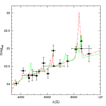
Figure 16: Qso synthetic template fitted over Combo17 magnitudes for J033219.5-275406. Solid curve is the z=0.28 solution and dashed curve is the z=0.70 solution.

A remarkable more compact structure (Structure 9-1) is detected inside this wall. This is the only compact structure detected in this wall (Structure 10 being perhaps an infalling group on the wall). Well sampled with 11 redshifts, Structure 9-1 has a filamentary structure (see Fig.15) and a velocity dispersion of 344$\pm$171 km/s. This would be typical of a group of galaxies, however, we have no firm indication of a possible X-ray emission because this source is just at the limit of the area covered by the Chandra data of Giacconi et al. (2002). However, these data show an X-ray source (J033219.5-275406, XID 249 in Giacconi et al. 2002) corresponding to a bright galaxy close to Structure 9-1. This X-ray source has a hard spectrum typical from an AGN and also have a radio counterpart: NVSS J033219-275406. The optical counterpart object is located at the end of the filament designed by Structure 9-1. We do not have any spectroscopic redshift for this object, however, when computing a photometric redshift, the best fit is obtained for a QSO template, also acting in favor of an ”active” object. There is two solutions in redshift: 0.28 and 0.70 (see Fig.16). The redshift of this object is determined by an emission enhancement around 8250A. Associating H$\alpha$ with this emission will give z=0.28 and associating H$\beta$ will give z=0.70 (in agreement with the Structure 9-1 redshift).

The galaxies detected in Structure 9-1 both have emission and absorption lines and are classified as late type galaxies using photometric and morphological types. The CMR of Structure 9-1 appears also poorly defined. This structure has 1.5 more emission line galaxies than the field at the same redshift and the same number of absorption line galaxies. The same tendency is visible using photometric and morphological types. The galaxy content of this structure is therefore quite late and similar to the field (using morphological types, Structure 9-1 galaxy content is different from the field galaxy content in the A/C diagram only at the 56$\%$ level). Moreover, Structure 9-1 presents an interesting chain morphology very different from the axisymmetric usual cluster/group shape. Finally, this structure is not detectable in galaxy density or color maps (using photometric redshifts).

The structure we have detected seems to be a peculiar case, quite similar to the highly anisotropic compact and moderatly massive structures proposed by West (1994) that are possibly the progenitors of the giant nearby elliptical galaxies or of the nearby fossil groups (e.g. Jones et al. 2003).

Table 1: Number of galaxies in cluster and in the field (along the cluster line of sight) down to I${}^{*}_{AB}$+2 for z=0.5 and down to I${}^{*}_{AB}$ for z=1 for a Coma-like cluster and for several areas. We used I${}^{*}_{AB}$$\sim$20.2 at z=0.5 and I${}^{*}_{AB}$$\sim$22.7 at z=1.

Considered angular size	0.8’$\times$0.8’	2’$\times$2’	6’$\times$6’	9.5’$\times$9.5’
Corresponding physical size at z=0.5	290kpc$\times$290kpc	730kpc$\times$730kpc	2200kpc$\times$2200kpc	3480kpc$\times$3480kpc
Cluster/field ratio at z=0.5	11/5	36/32	108/288	127/720
Considered angular size	0.7’$\times$0.7’	1.7’$\times$1.7’	5’$\times$5’	7.5’$\times$7.5’
Corresponding physical size at z=1	340kpc$\times$340kpc	820kpc$\times$820kpc	2400kpc$\times$2400kpc	3600kpc$\times$3600kpc
Cluster/field ratio at z=1	11/5	36/32	108/275	127/618

Table 2: Elliptical galaxy colors for several redshifts. Magnitude bands are chosen to emcompass the 4000$\AA$ break given the redshift.

	B-V	V-R	R-I
z=0.2	1.15
z=0.4	2.20	1.25
z=0.6		1.16	1.31
z=0.8			1.77
z=1.0			1.81
z=1.2			1.78

Table 3: Number of expected measured galaxies in clusters with various velocity dispersions as a function of the Global Sampling Rate (GSR). Values are given for z=0.73 and z=1.10.

z	GSR	400km/s	600km/s	900km/s
0.73	12$\%$	12	12	12
0.73	23$\%$	20	23	23
0.73	33$\%$	30	30	30
0.73	43$\%$	35	43	48
1.10	12$\%$	2	7	6
1.10	23$\%$	5	11	10
1.10	33$\%$	9	13	17
1.10	43$\%$	16	15	22

Table 4: Structures detected with coordinates (if not extended over the whole field of view), mean redshift, velocity dispersion (km/s: vd) and its 1-$\sigma$ error, number of galaxies with a redshift belonging to the structure, physical size (kpc), X-ray id from Giacconi et al. (2002), Kolmogorov Smirnov percentage (KS1) with the considered color-magnitude space, Kolmogorov Smirnov percentage (KS2) within the A/C space (when more than 5 galaxies provided such a classification) and Class following Section 5.

Id	alpha	delta	z	vd	Error	N	size	Xid Giacconi	KS1	KS2	Class
				km/s	km/s		kpc
1	03 32 35.2	-27 45 11.9	0.215	467	196	11	699	-	99$\%$ B/B-V	11$\%$	3
2	03 32 14.5	-27 48 39.2	0.227	265	89	5	658	-	41$\%$ B/B-V	7$\%$	4
3	03 32 32.1	-27 42 08.4	0.312	509	345	5	620	-	97$\%$ B/B-V		3
4	03 32 11.0	-27 41 49.8	0.420	376	259	7	608	-	93$\%$ B/B-V		3
5	03 32 07.6	-27 44 09.0	0.544	384	127	5	700	-	64$\%$ V/V-R	45$\%$	4
6	03 32 01.2	-27 45 19.2	0.576	312	97	5	677	-	96$\%$ V/V-R		4
7	03 32 29.1	-27 55 55.9	0.619	340	148	9	1314	-	96$\%$ V/V-R		3
8	03 31 55.4	-27 41 51.9	0.621	398	125	5	702	out of field	70$\%$ V/V-R		4
9			0.660	1269	181	66	$\sim$8000	-	85$\%$ V/V-R	9$\%$	Wall
10	03 32 28.8	-27 52 46.8	0.681	320	82	5	639	-	69$\%$ V/V-R	12$\%$	3
11			0.735	665	116	145	$\sim$9000	-	99$\%$ R/R-I	6$\%$	Wall
12	03 32 17.6	-27 42 48.4	0.978	280	145	6	618	-	38$\%$ R/R-I		4
13	03 32 29.7	-27 43 01.0	1.036	329	289	7	1147	-	71$\%$ R/R-I		3
14	03 32 16.6	-27 51 51.9	1.044	154	84	7	731	-	77$\%$ R/R-I		3
15	03 32 14.7	-27 52 58.7	1.098	373	131	12	440	87 and 51	94$\%$ R/R-I		1
16	03 32 19.8	-27 46 23.52	1.221	161	149	6	791	-	53$\%$ R/R-I		3
17	03 32 22.3	-27 45 14.7	1.306	224	100	5	866	-	57$\%$ R/R-I		3

Table 5: Structures detected inside the z=0.66 and z=0.735 walls. Same label as Table 4.

Id	alpha	delta	z	vd	Error	N	size	Xid Giacconi	KS1	KS2	Class
				km/s	km/s		kpc
9-1	03 32 32.8	-27 59 08.5	0.660	344	171	11	723	641	64$\%$ V/V-R	56$\%$	2
11-1	03 32 20.7	-27 46 05.7	0.736	455	161	10	941	566	99$\%$ V/V-R	99$\%$	1
11-2	03 31 55.9	-27 54 35.2	0.736	496	132	5	659	-	42$\%$ V/V-R		3
11-3	03 32 27.5	-27 41 18.0	0.734	157	53	6	376	-	11$\%$ V/V-R		3
11-4	03 32 51.8	-27 42 55.0	0.732	315	63	6	800	-	85$\%$ V/V-R		3
11-5	03 32 54.4	-27 54 22.6	0.736	399	143	5	800	-	59$\%$ V/V-R		3

5 Discussion and Conclusions

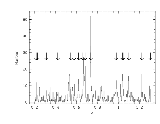
Figure 17: Redshift histogram of the galaxies along the CDFS line of sight. Redshift location of the detected structures are shown as arrows.

We detected 17 compact structures (Structure 11 being a compact wall split in 5 smaller structures: see Table 5) and 1 more diffuse wall including one of the compact structures. These structures are distributed all across the CDFS field of view and have redshifts generally in good agreement with the redshift peaks of the histogram of all galaxies along the CDFS line of sight (Fig. 17).

We detected a chain-like structure embedded in a quite diffuse wall at z=0.66 (structure 9-1) showing signs of ongoing collapse and perhaps similar to the progenitors of giant nearby elliptical galaxies.

We also have detected a dense wall at z$\sim$0.735, very compact in redshift space and extending all across the field of view. The existence of such extended and compact structures in redshift space is remarquable as the thickness of the structure in redshift space is very small for a non-virialized structure. However, as outlined for example by Kaiser (1987), such structures have probably a strongly anisotropic clustering pattern. This results in a compression of the structure along the line of sight, making these structures appear thinner in redshift space than in real space (while in more massive and dense virialized structures as clusters of galaxies, the effect in reversed, forming the well known “fingers of god”). This structure is interpreted as a central core (Structure 11-1) and an accretion area composed of several bodies.

Among the structures we detected, we distinguish 4 classes:

- 2 are real groups of galaxies (class 1): Structure 11-1 and 15

- 1 is a partially evolved and low mass structure of galaxies (class 2): Structure 9

- 12 are proto-clusters/groups of galaxies (class 3): Structures 1, 3, 4, 7, 10, 11-2, 11-3, 11-4, 11-5, 13, 14, 16 and 17

- 5 are very early formation stage or fake structures of galaxies (class 4): Structures 2, 5, 6, 8 and 12

Several arguments have already been discussed to check the “reality” of these detected structures. In addition, we can discuss statistically the redshift distribution of the identified structures. The more relaxed a real structure will be, the more gaussian the structure galaxy redshift distribution will appear. Due to small numbers inside every individual group, we built synthetic distributions by rescaling the redshift distributions of each structure: each redshift was scaled using the mean redshift and the velocity dispersion of the structure (see also Adami et al. 1998b). We defined 3 subsamples: class 1 and 2 structures (50 galaxies), class 3 structures (67 galaxies) and class 4 structures (20 galaxies). First, using Kolmogorov-Smirnov tests, we look for differences between the normalized redshift distributions comparing each of them to the other two. Class 1+2 and class 3 sub-samples will only differ at the 77$\%$ level (not very significant) while the class 4 sub-sample differs at the 99$\%$ level from class 1+2 and from class 3 sub-samples. Moreover, fitting a gaussian to class 1+2 and class 3 sub-samples gives a reasonnable agreement, while it clearly fails for class 4 sub-sample. Therefore, class 4 sub-sample is possibly constituted of, at least, partly of fake structures.

The majority of the detected structures has a poorly defined red sequence in the CMR, but significantly different from the field galaxy population. In the hierarchical scenario, one would expect less evolved structures with increasing redshift, with the distant ones more similar to field galaxies in the color-magnitude diagram, but it has to be taken into account the selection bias that richer structures are preferentially detected with increasing redshift.

We also note that the structures detected at z$\geq$0.9 have a lower velocity dispersion compared to the lower redshift sample: 254km/s versus 370km/s. Expressed in other terms the mean velocity dispersion of the z$\leq$0.9 structures is equal to the maximal velocity dispersion of the z$\geq$0.9 structures. This would be consistent with the fact that we expect less and less massive structures as the redshift is increasing (e.g. Evrard et al. 2002). We also expect, however, the detection of more and more young structures with increasing redshift, having, therefore, an artificially increased velocity dispersion. This would imply an even stronger amplitude in our observed velocity dispersion decrease with redshift.

Our sample field of view is by far too small in order to efficiently constrain cosmological models using structure counts. However, it is interesting to note that recent cosmological simulations (e.g. Evrard et al. 2002) predict numbers for LCDM models in good agreement with our detections. Evrard et al. (2002) predict for example between 1 and 4 structures more massive than 5 10¹³ solar mass in our field of view (a $\tau$CDM model would predict 0 following Evrard et al.). Using for example Girardi et al. (2002), such a mass is typical of Structure 15, being the only such one in our sample at z greater than 1. Similarly, Evrard et al. (2002) predict no cluster at all more massive than 3 10¹⁴ solar mass in our field of view at z greater than 1 and we detect no such clusters. Similar analyses will have,however, to be performed on larger areas in order to give a reliable answer.

Figure 14: HST I image of Structure 15 with galaxies associated to the structure (small circles) and the two X-ray sources (large circles). Size of the image is 3.7’$\times$2.8’.

Figure 15: HST I image of Structure 9-1 with galaxies associated to the structure (small circles) and the two X-ray sources (larges circles). Image size is 5.5’$\times$3.3’.

References

- (1) Abell G.O., Corwin H.G., Olowin R.P., 1989, ApJS 70, 1
- (2) Adami C., Mazure A., 2002, AA 381, 420
- (3) Adami C., Mazure A., Biviano A., Katgert P., Rhee G., 1998, AA 331, 493 (a)
- (4) Adami C., Biviano A., Mazure A., 1998, AA 331, 439 (b)
- (5) Arnouts S., Vandame B., Benoist C., et al., 2001, AA 379, 740
- (6) Baum W., 1959, PASP 71, 106
- (7) Beers T., Flyn K., Gebhardt K., 1990, AJ 100, 32
- (8) Bershady M.A., Jangren A., Conselice C., 2000, AJ 119, 2645
- (9) Biviano A., Durret F., Gerbal D., et al., 1996, AA 311, 95
- (10) Biviano A., Katgert P., Thomas T., 2002, AA 387, 8
- (11) Bottini D., Garilli B., Maccagni D., et al., 2005, AA in press
- (12) Castander F.J., 1998, ApSS 263, 91
- (13) Cimatti A., Daddi E., Mignoli M., et al., 2002, AA 381, L68
- (14) Dressler A., Smail I., Poggianti B., 1999, ApJS 110, 213
- (15) Davé R., Hellinger D., Primack J., Nolthenius R., Klypin A., 1997, MNRAS 284, 607
- (16) Evrard A.E., MacFarland T.J., Couchman H.M.P., et al., 2002, ApJ 573, 7
- (17) Folkes S., Ronen S., Price I., et al., 1999, MNRAS 308, 459
- (18) Giacconi R., Zirm A., Wang J.X., et al., 2002, ApJSS 139, 369
- (19) Giavalisco M., Dickinson M., Ferguson H.C., et al., 2004, ApJ 600, L93
- (20) Gilli R., Cimatti A., Daddi E., et al., 2003, ApJ 592, 721
- (21) Girardi M., Manzato P., Mezzetti M., et al., 2002, ApJ 569, 720
- (22) Ilbert O., et al., 2005, AA in preparation
- (23) Jones L.R., Ponman T.J., Horton A., et al., 2003, MNRAS 343, 627
- (24) Kaiser N. 1987, MNRAS 227, 1
- (25) Lauger S., et al., 2005, AA in preparation
- (26) Lax D. 1985, J. Am. Stat. Assoc. 80, 736
- (27) Le Fèvre O., Vettolani G., Paltani S., et al., 2004, AA 428, 1043
- (28) Mazure A., Katgert P., den Hartog R., et al., 1996, AA 310, 31
- (29) Moy E., Barmby P., Rigopoulou D., et al., 2003, AA 403, 493
- (30) Rizzo D., Adami C., Bardelli S., et al., 2004, AA 413, 453
- (31) Romer A.K., Viana P.T.P.., Liddle A.R., Mann R.G., 2001, ApJ 547, 594
- (32) Sandage A., 1972, ApJ 176, 21
- (33) Scaramella R., Bottini D., Garilli B., et al., 2006, AA in preparation
- (34) Serna A., Gerbal D., 1996, AA 309, 65
- (35) Szokoly G.P., Bergeron J., Hasinger G., et al., 2004, ApJS 155, 271
- (36) West M.J., 1994, MNRAS 268, 79
- (37) Wolf C., Meisenheiner K., Kleinheinrich M., et al. 2004, AA, submitted astro-ph: 0403666