Relativistic Ionization Fronts

Abstract

We derive the equations for the propagation of relativistic ionization fronts (I-fronts) in both static and moving gases, including the cosmologically-expanding intergalactic medium (IGM). We focus on the supersonic R-type phase that occurs right after a source turns on, and we compare the nonrelativistic and relativistic solutions for several important cases. Relativistic corrections can be significant up until the light-crossing time of the equilibrium Strömgren sphere. When $q,$ the ratio of this light-crossing time and the recombination time, exceeds unity, the time for the expanding I-front to reach the Strömgren radius is delayed by a factor of $q$. For a static medium, we obtain exact analytical solutions and apply them to the illustrative problems of an O star in a molecular cloud and a starburst in a high-redshift cosmological halo. Relativistic corrections can be important at early times when the H II regions are small, as well as at later times, if a density gradient causes the I-front to accelerate. For the cosmologically-expanding IGM, we derive an analytical solution in the case of a steady source and a constant clumping factor. Here relativistic corrections are significant for short-lived, highly-luminous sources like QSOs at the end of reionization ($z\simeq 6$), but negligible for weaker or higher-redshift sources. Finally, we numerically calculate the evolution of relativistic I-fronts in the presence of small-scale structure and infall, for a large galaxy undergoing a starburst and a luminous, high-redshift QSO. For such strong and short-lived ($z\sim 7$) sources, the relativistic corrections are quite significant, and small-scale structure can decrease the size of the H II region by up to an additional $\sim 25$%. However, most of the IGM was ionized by smaller, higher redshift sources. Thus the impact of relativistic corrections on global reionization is small and can usually be neglected.

1 Introduction

Ionization fronts are ubiquitous in astrophysics. On interstellar scales, they occur when new stars form in molecular clouds, and their propagation has important dynamical effects on the surrounding medium. The compact and ultra-compact H II regions that form in this way have been extensively studied both theoretically and observationally (for recent detailed reviews and further references see e.g. Garay & Lizano 1999; Evans 1999; Churchwell 2002). Radiative feedback effects play a key role in determining the physical conditions in star-forming regions, with profound effects on the star-formation rates and efficiencies, and the resulting initial mass function. For example, ionization fronts may trigger star formation in dense clumps through compression and subsequent cooling of the gas (e.g. Lefloch et al. 1997; Hosokawa & Inutsuka 2005; Lee et al. 2005).

On larger scales, the propagation of ionization fronts has emerged as one of the key problems in cosmology. Shapiro & Giroux (1987) pointed out that the first sources of ionizing radiation in the post-recombination expanding universe, be they quasars, primeval galaxies, or some pregalactic objects like Population III stars, would have caused cosmological I-fronts to sweep outward into the surrounding intergalactic medium (IGM), and they derived the equations to describe their propagation. These I-fronts, they found, were generally weak, R-type fronts that moved supersonically with respect to both the neutral gas ahead of them and the ionized gas behind, thereby racing ahead of the hydrodynamical response of the ionized gas. The H II regions created by these expanding cosmological I-fronts generally do not fill their “Strömgren spheres” – i.e. a fully-ionized sphere whose size is just large enough to encompass as many atoms recombining per second as there are ionizing photons emitted per second by the central source .

The origin of this difference between the cosmological I-fronts and their interstellar counterparts is the ever-decreasing mean gas density in the cosmological case. The predominance of this R-type phase in the cosmological case has made it possible to approximate the propagation of the global I-fronts believed responsible for the reionization of the universe by a “static limit” in which the evolving inhomogeneous density field of the IGM is assumed to be predetermined by large-scale structure formation, neglecting the hydrodynamical response of the gas to its ionization (e.g. Ciardi et al. 2000; Sokasian et al. 2003). On small scales, where gas can be much denser than average, such as inside halos, this “static” approximation can break down as the I-fronts decelerate to about twice the sound speed of the ionized gas and transform from supersonic R-type to subsonic D-type, thereby coupling their fate to the dynamical response of the ionized gas. Some attempt has also been made to study this dynamical phase of cosmic reionization I-fronts, by “zooming in” on the gas dynamics of the I-front as it encounters individual halos (e.g. Shapiro, Iliev, & Raga 2004; Iliev, Shapiro, & Raga 2005b) or by relaxing the “static approximation” referred to above while simulating large-scale structure formation during global reionization (Gnedin 2000; Ricotti et al. 2002). Here the primary issue has been to characterize the onset, duration, and topology of reionization (Gnedin 2000; Bruscoli, Ferrara, & Scannapieco 2002; Haiman & Holder 2003; Wyithe & Loeb 2003; Ciardi, Stoehr, & White 2003; Furlanetto, Zaldarriaga, & Hernquist 2004; Iliev, Scannapieco, & Shapiro 2005a), particularly in light of the discrepancy between the epoch of reionization $z\mathrel{\hbox{\hbox to0.0pt{\hbox{\lower 4.0pt\hbox{$\sim$}}\hss}\hbox{$>$}}}15$ favored by the first-year data from the Wilkinson Microwave Anisotropy Probe (Kogut et al. 2003), and observations of a Gunn-Peterson trough in high-redshift quasars, which suggest that reionization did not end until $z\sim 6$ (White et al. 2003; Fan et al. 2004). Other important questions include the growth of individual ionized regions around high-redshift Lyman-alpha emitters (Haiman 2002; Santos 2004), which would otherwise be highly obscured by neutral gas (Malhotra & Rhoads 2004; Stern et al. 2005), and the relationship between the proximity effect around high-redshift quasars and the mean IGM neutral fraction at this redshift (Wyithe & Loeb 2004; Oh & Furlanetto 2005; Yu & Lu 2005).

Until recently, the I-fronts described above have been treated nonrelativistically, as if the speed of light were infinite. Unlike shock fronts, which can reach relativistic (Rel) speeds only in the most extreme environments where the energy density is very high, such that the kinetic energy per baryon is comparable to or greater than its rest mass energy, ionization fronts are intrinsically radiative phenomena that are mediated by the propagation of photons. This means that even the weakest ionizing source may, in principle, drive a strongly relativistic I-front. Thus the finite speed of light is always an issue for I-front propagation, whose importance should be ascertained for each set of astrophysical circumstances.

Nevertheless, relativistic I-fronts have received only limited treatment in the literature. Roughly speaking, the I-front will be relativistic whenever the photon to atom ratio at the front exceeds unity. This occurs whenever a source releases ionizing photons faster than a surface moving outward at the speed of light can overtake as many neutral atoms. The equations of Shapiro & Giroux (1987) for the evolution of the spherical I-front around a point source in the cosmologically-expanding IGM show that, at early times close to source turn-on, the nonrelativistic (NR) treatment formally yields an I-front speed which exceeds the speed of light, for just this reason. This “superluminal” phase is generally so short-lived, lasting only a tiny fraction of the age of the universe at source turn-on, that it has a negligible effect on the overall evolution of the I-front for a steady source. Recently, however, interest in this brief, early phase of the I-front has been drawn by observations of the spectra of high redshift quasars and Lyman alpha line emitters at redshifts $z>6$ which suggest that we are seeing each of these sources as if it is surrounded by an isolated intergalactic H II region of its own making. In the quasar case, in particular, assumptions that the source of ionizing radiation is the observed quasar, itself, and that quasar lifetimes are much less than the age of the universe at those epochs, combine to suggest that the relativistic phase of the I-front predicted by the nonrelativistic solutions is quite relevant. For this reason, White et al. (2003) presented a revised equation for the expansion speed of the spherical I-front which takes account of the finite speed of light, although it neglects recombinations. They noted, however, that the relationship between the apparent size of the H II region along the line of sight and the parameters on which the physical evolution of that size depends, namely the quasar’s luminosity and the average density of neutral H atoms in the IGM outside the H II region, are exactly the same as would be achieved by applying the equations of Shapiro & Giroux (1987). This surprising result is apparent also in the treatments of Yu (2005) and Yu & Lu (2005), who discussed the effect of relativistic expansion on the apparent shape of a cosmological H II region around a high-redshift QSO, including the effects of recombination. It results from the fact that the photons in the observed quasar spectrum at the redshifted wavelength which marks the outer edge of the H II region were emitted by the QSO at the retarded time equal to the time those photons reached the I-front, minus their light-travel time from the source. Using this retarded time to evaluate the I-front radius in the equations of Shapiro & Giroux (1987) automatically accounts properly for the finite speed of light.

These recent discussions of the QSO H II regions state their basic H II radius evolution equation without derivation and do not explain its connection to the fundamental conservation equations for an I-front, namely, the I-front continuity jump condition and the equation of radiative transfer for the ionizing photons. In what follows, we will start from those fundamental conservation equations to take full account of special relativity in generalizing them to address a wider range of circumstances and make clear the derivation that underlies the evolution equation for the spherically symmetric H II regions mentioned above. We will examine the general problem of relativistic I-fronts, in both static, moving, and cosmologically-expanding media, deriving a number of exact and universal solutions and assessing the importance of relativistic effects in both the interstellar medium and cosmology.

The structure of this work is as follows. The relativistic equations for I-front evolution in a general form are derived in § 2 for a source in a moving gas. In § 3 we use these equations to describe the relativistic evolution of a spherical I-front surrounding a point source in a static medium, deriving some exact analytic solutions to this problem, for a uniform gas density and a density that varies as a power-law in radius. For illustration, we apply these to a front expanding around an O-star or OB association in a molecular cloud and to a front inside a cosmological halo. We also present a numerical solution for the I-front around a point source in a plane-stratified medium. In § 4 we generalize the equations of Shapiro & Giroux (1987) for the cosmological I-front around a point source in an expanding IGM to take account of special relativity, finding an exact analytical solution, as well, which we use to assess the importance of relativistic effects as a function of redshift and source flux. In § 5, we present numerical solutions for the isolated H II regions around cosmological sources, which include the effect of small-scale cosmological structure (i.e. self-shielding minihalos, time-varying clumping factor for the diffuse IGM, and the infall of gas surrounding each source halo) on these intergalactic I-fronts. We apply these solutions to determine the impact of relativistic effects on global cosmic reionization, by the approach described in Iliev et al. (2005a), which evolves the I-fronts created by a statistical distribution of cosmological ionization sources to the point at which their H II regions finally overlap. Our conclusions are summarized in § 6.

2 Basic Equations

2.1 Relativistic I-front in a Moving Gas

Consider the motion of an I-front through some gas that is itself moving with respect to the source of the ionizing radiation. In the lab frame defined as the rest frame of the source, the I-front moves with velocity ${\bf v}_{I}\equiv{\bf\beta}_{I}c$, while the gas just outside the I-front on the neutral side (side “1”) moves with velocity ${\bf v}_{g,1}\equiv{\bf\beta}_{g,1}c$. Assume that ${\bf v}_{I}$ and ${\bf v}_{g,1}$ are in the same direction, so the motion is one-dimensional. The relativistic law for the addition of velocities then gives the velocity of the I-front as measured in the rest frame of the gas just outside the front, $v_{I}^{\prime}=\beta_{I}^{\prime}c$, according to

$$v_{I}^{\prime}=\frac{v_{I}-v_{g,1}}{1-v_{I}v_{g,1}/c^{2}}.$$ (1)

In the rest frame of the I-front, the gas moves with velocity $v_{g,1}^{\prime\prime}=\beta^{\prime\prime}_{g,1}c=-v_{I}^{\prime}=-\beta_{I}^{\prime}c,$ where here and below double primed variables are quantities measured in the frame of the front.

2.2 I-front Continuity Jump Condition

The relativistic I-front continuity jump condition, which expresses the balance between the flux of ionizing photons arriving at the front and the flux of atoms that are ionized by those photons as the atoms pass through the front, is written in the rest frame of the I-front as follows:

$$n_{H,1}^{\prime\prime}v_{g,1}^{\prime\prime}=\beta_{i}^{-1}F^{\prime\prime},$$ (2)

where $v_{g,1}^{\prime\prime}$ is the front velocity relative to the undisturbed gas into which the front is moving, given by $v_{I,1}^{\prime}$ in equation (1). To get the density $n_{H,1}^{\prime\prime}$, we take the value measured in the rest frame of the I-front,

$$n_{H,1}^{\prime\prime}=\gamma_{g,1}^{\prime\prime}n_{H,1}^{\prime}=\gamma_{I}^{\prime}n_{H,1}^{\prime},$$ (3)

where the Lorentz factors, $\gamma$, are related to the velocities, $\beta c$, by $\gamma\equiv(1-\beta^{2})^{-1}$, as usual. The quantity $\beta_{i}$ counts the number of ionizing photons required to yield a single newly ionized H atom on the ionized side of the front and is thus frame-independent.

The ionizing photon flux $F^{\prime\prime}$ as measured by the moving front is different from the lab-frame flux $F$ measured in the frame of the source, by a Lorentz-boost to the frame moving with velocity $v_{I}$ in the lab frame:

$$F^{\prime\prime}=\gamma_{I}(1-\beta_{I})F$$ (4)

(Shapiro, Milgrom, & Rees 1986), where we have implicitly assumed that the relativistic Doppler shift of the photons from the lab frame to the rest frame of the moving gas does not significantly affect the integrated number of ionizing photons in the incident flux. Otherwise, we should replace $F$ in equation (4) by the modified flux which counts only those photons at the location of the I-front at lab frame frequencies $\nu$ such that $\nu\gg\nu_{min}$, where

$$\nu_{min}=\nu_{th}\gamma_{g,1}(1+\beta_{g,1}),$$ (5)

where $\nu_{th}$ is the threshold frequency for ionizing $H$ atoms from the ground state.

Combining equations (1) and (2)-(4) yields the equation for the I-front velocity in the lab frame as follows:

$$\beta_{I}=\left[\frac{(1-\beta_{I}\beta_{g,1})\gamma_{g,1}}{\gamma_{I}^{\prime}}\right]\left[\frac{\gamma_{I}(1-\beta_{I})F}{\beta_{i}n_{H,1}c}\right]+\beta_{g,1}$$ (6)

We have also used the fact that the lab frame $H$ atom density $n_{H,1}$ is related to the value in the rest frame of the gas, according to

$$n_{H,1}=n_{H,1}^{\prime}\gamma_{g,1}.$$ (7)

2.3 Radiative Transfer of Ionizing Flux Across H II Region

2.3.1 Optical Depth

Ionizing photons traveling radially outward from the central source will suffer absorptions due to the residual bound-free opacity of gas on the ionized side of the I-front, inside the H II region. As these photons cross a spherical shell of radius $dr$ as measured in the lab frame (i.e. rest frame of source), in which frame the H atom number density is $n_{H}(r)$ and the frame-independent neutral fraction is $(1-x)$, the probability that a photon emitted at a frequency $\nu$ in the lab frame is absorbed is given for a shell that expands away from the source at velocity $v_{g}(r)=\beta_{g}(r)c$, by optical depth $d\tau$, according to:

$$d\tau_{\nu}=n_{H}(1-x)\sigma_{\nu^{\prime}}(1-\beta_{g})dr,$$ (8)

where $\sigma_{\nu^{\prime}}$ is the photoionization cross section of an H atom in the ground state, evaluated at photon frequency $\nu^{\prime}=\gamma_{g}(1-\beta_{g})\nu$, the frequency in the comoving frame of the expanding shell (Shapiro et al. 1986).

2.3.2 Ionization Equilibrium

For gas in the expanding shell, ionization equilibrium in the “on-the-spot” approximation, in which radiative recombinations to atomic levels $n\geq 2$ are balanced by photoionizations from the ground state, gives the neutral fraction according to

$$\frac{1-x}{x^{2}}=\frac{\alpha_{B}(n_{H}^{\prime})^{2}}{n_{H}^{\prime}\overline{\sigma}F^{\prime}}=\frac{\alpha_{B}n_{H}^{\prime}}{\overline{\sigma}F^{\prime}},$$ (9)

where $\overline{\sigma}$ is the frequency-averaged bound-free cross-section for frequencies $\nu^{\prime}\geq\nu_{th}$, weighted by the flux of photons at each frequency, and where the primed quantities are measured in the comoving frame of the gas. The atomic number density and the photon flux in this frame are related to their counterparts in the lab frame according to

$$n_{H}^{\prime}=n_{H}/\gamma_{g},$$ (10)

and

$$F^{\prime}=\gamma_{g}(1-\beta_{g})F,$$ (11)

where $F$ should be the photon flux for $\nu\geq\gamma_{g}(1+\beta_{g})\nu_{th}$ (Shapiro et al. 1986). Equations (9)-(11) yield

$$\frac{1-x}{x^{2}}=\frac{\alpha_{B}n_{H}}{\overline{\sigma}\gamma_{g}^{2}(1-\beta_{g})F}.$$ (12)

According to equations (8) and (12), the optical depth through the shell is given, therefore, by

$$d\tau_{\nu}=\left(\frac{\sigma_{\nu^{\prime}}}{\overline{\sigma}}\right)\left(\frac{\alpha_{B}x^{2}n_{H}^{2}}{\gamma_{g}^{2}F}\right)dr.$$ (13)

2.3.3 Flux Variation With Distance From Source

Consider the lab frame quantity $S(r,t_{R})=4\pi r^{2}F(r,t)$, which is the rate at which ionizing photons pass through a shell of radius $r$ at time $t$ that were emitted by the source at the retarded time $t_{R}\equiv t-r/c$. The quantity $S(0,t)$ is the ionizing photon luminosity of the source at time $t$. If the source luminosity is $L_{\nu}\,(\rm erg\,s^{-1}Hz^{-1})$ in the lab frame, then

$$S(0)=\dot{N}_{\gamma}\equiv\int_{\nu_{\rm th}}^{\infty}\dot{N}_{\gamma,\nu}d\nu\equiv\int_{\nu_{\rm th}}^{\infty}\frac{L_{\nu}}{h\nu}d\nu.$$ (14)

In the absence of opacity due to photoionization, the quantity $S(r,t_{R})$ is independent of $r$. The effect of opacity is to attenuate $S(r,t_{R})$ as follows, using equation (13):

$$\frac{d}{dr}\left[4\pi r^{2}F_{\nu}(r)\right] = -\dot{N}_{\gamma,\nu}(t_{R})e^{-\tau_{\nu}}\frac{d\tau_{\nu}}{dr}$$ (15)

$$= -\left[4\pi r^{2}F_{\nu}(r)\right]\left[\left(\frac{\sigma_{\nu^{\prime}}}{\overline{\sigma}}\right)\left(\frac{\alpha_{B}x^{2}n_{H}^{2}}{\gamma_{g}^{2}F}\right)\right].$$

Multiplying both sides of equation (15) by $d\nu$ and integrating over all frequencies $\nu\geq\gamma_{g}(1+\beta_{g})\nu_{th}$ yields

$$\frac{dS}{dr}=-4\pi r^{2}\alpha_{B}x^{2}n_{H}^{2}\gamma_{g}^{-2}.$$ (16)

We can integrate this over radius to yield $S(r_{I},t_{R,I})$ at the location of the I-front according to

$$S(r_{I},t_{R,I})=S(0,t_{R,I})-\int_{0}^{r_{I}}dr\cdot 4\pi r^{2}xn_{e}n_{H}\gamma_{g}^{-2}\alpha_{B},$$ (17)

where $t_{R,I}\equiv t_{R}(r=r_{I})$ and we evaluate the quantities inside the integral on the right-hand-side at the time $t(r)\equiv t_{R,I}+r/c$. We have also replaced one of the factors of $xn_{H}$ by $n_{e}$ above. Although we have neglected the presence of helium until now, we can account for the contributions of ionized helium to the electron density inside the H II region by writing $n_{e}=\chi_{\rm eff}xn_{H}$, where $\chi_{\rm eff}\equiv 1+pA({\rm He})$, $A({\rm He})=0.08$ is the He abundance by number with respect to hydrogen, and $p=0,1$ or 2 according to whether He is mostly neutral, singly ionized or doubly ionized, respectively. If we also allow for a volume-averaged clumping factor, $C=\langle n_{H}^{2}\rangle/\langle n_{H}\rangle^{2}$, then equation (17) becomes

$$S(r_{I},t_{R,I})=\dot{N}_{\gamma}(t_{R,I})-\int_{0}^{r_{I}}dr\cdot 4\pi r^{2}\chi_{\rm eff}x^{2}n_{H}^{2}\gamma_{g}^{-2}\alpha_{B}C.$$ (18)

Here $\alpha_{B}=2.59\times 10^{-13}$ cm³ s^-1 is the case B recombination coefficient for hydrogen at $10^{4}$ K (which is the temperature we assume for the ionized medium throughout this paper). The value of the radius $r_{I}$ which makes $S(r_{I},t_{R,I})$ vanish according to equation (18) is then the Strömgren radius $r_{S}$. Hereafter, unless otherwise noted, the only retarded time to which we shall refer will be $t_{R,I}$, and we shall drop the subscript “I” when referring to it. The lab frame flux at the front at time $t$ is then given by

$$F(r_{I},t)=\frac{S(r_{I},t_{R})}{4\pi r_{I}^{2}}.$$ (19)

While the analysis in § 2 apparently applies to a point source of ionizing radiation surrounded by a spherically-symmetric gas, it actually applies equally well to the general case of inhomogeneous gas which varies in all three spatial dimensions. In the latter case, we simply interpret the equations as if they are written in $(r,\theta,\phi)$ spherical coordinates centered on the source, as long as any non-radial gas motions which might be present are subrelativistic. If a problem arises in which relativistic, non-radial gas motions occur, the equations above should be appropriately modified to account for the effect of transverse velocity on the relativistic transformations, as well. In the absence of such relativistic transverse gas motion, however, we can use the analysis presented in this section for the general 3D problem without modification.

3 Relativistic I-fronts in Static Media

3.1 Point Source in a Static Medium

Consider a point source in a static gas. In this case, $v_{g,1}=0$, the velocity of the I-front $v_{I}^{\prime}$ in the frame of the undisturbed gas ahead of the front is just the same as its velocity $v_{I}$ in the lab frame in which the source is at rest, and $\gamma_{I}^{\prime}=\gamma_{I}$. In the frame of the front, therefore, $v_{g,1}^{\prime\prime}=-v_{I}$, the H atom density $n_{H,1}^{\prime\prime}=\gamma_{I}n_{H,1}$, and the flux $F^{\prime\prime}$ is related to the lab frame flux $F$ by equation (4). Equation (6) for the front velocity in the lab frame then becomes

$$\beta_{I}=\frac{F}{\beta_{i}n_{H,1}c+F},$$ (20)

where $F$ is the number flux of ionizing photons at the current position of the I-front, given by equation (18) with $\gamma_{g}=1$ and equation (19).

Combining equations (18) - (20) and solving for ${\rm v}_{I}$, we obtain the lab frame evolution equation for the radius $r_{I}$ of the spherical I-front,

$$\frac{dr_{I}}{dt}=c\frac{\dot{N}_{\gamma}(t_{R})-4\pi\int_{0}^{r_{I}}{n_{H}}^{2}C\alpha_{B}\chi_{\rm eff}r^{2}dr}{4\pi\beta_{i}cr_{I}^{2}n_{H,1}+\dot{N}_{\gamma}(t_{R})-4\pi\int_{0}^{r_{I}}{n_{H}}^{2}C\alpha_{B}\chi_{\rm eff}r^{2}dr}.$$ (21)

In the nonrelativistic limit in which $dr_{I}/dt\ll c$, the first term in the denominator becomes dominant and equation (21) reduces to the usual expression

$$\frac{dr_{I}}{dt}=\frac{\dot{N}_{\gamma}(t)-4\pi\int_{0}^{r_{I}}{n_{H}}^{2}C\alpha_{B}\chi_{\rm eff}r^{2}dr}{4\pi\beta_{i}r_{I}^{2}n_{H,1}}.$$ (22)

In the opposite, strongly relativistic limit, in which the flux is very large, both the denominator and numerator are dominated by the $\dot{N}_{\gamma}$ term and $dr_{I}/dt$ approaches $c$ asymptotically.

For this static medium, the I-front velocity equation can also be derived by imposing photon conservation within the ionized volume. This is done by requiring that at a time $t$ the total number of photons that have reached the ionization front is equal to the sum of the total number of atoms within the volume and the total number of recombinations that occurred within the volume excluding recombinations that affect emitted photons that have not yet reached $r_{I}(t)$, that is

$$\int_{0}^{t_{R}}\dot{N}_{\gamma}(t^{\prime})dt^{\prime} = 4\pi\beta_{i}\int_{0}^{r_{I}(t)}n_{H}(r)r^{2}dr$$ (23)

$$+ 4\pi\int_{0}^{t}dt^{\prime}\int_{0}^{r_{I}(t^{\prime})}n_{H}^{2}(r)C\alpha_{B}\chi_{\rm eff}r^{2}dr$$

$$- 4\pi\int_{0}^{t-t_{R}}dt^{\prime}\int_{0}^{ct^{\prime}}n_{H}^{2}(r)C\alpha_{B}\chi_{\rm eff}r^{2}dr$$

Differentiating this equation with respect to time, we obtain

$$\left[\dot{N}_{\gamma}(t_{R})-4\pi\int_{0}^{r_{I}}n_{H}^{2}(r)C\alpha_{B}\chi_{\rm eff}r^{2}dr\right]\left(1-\frac{\dot{r_{I}}}{c}\right)$$

$$=4\pi\beta_{i}\frac{dr_{I}}{dt}n_{H}(r_{I})r_{I}^{2},$$ (24)

and solving for $\dot{r}_{I}$ recovers equation (21).

For a given density field and time-dependent photon luminosity, equation (21) can, in principle, be solved to yield the I-front radius and radial velocity as explicit functions of time $t$, for any direction $(\theta,\phi)$. We will do so for certain density profiles in the sections that follow. Before we consider such explicit solutions, however, we note that there is a simplification that results if we rewrite our equations in terms of the retarded time, $t_{R}$, rather than physical time, $t.$ For every interval $dt$ of physical time, there is a corresponding interval

$$dt_{R}=dt(1-\beta_{I}).$$ (25)

If we define a “retarded velocity” $\beta_{\rm I,R}\equiv c^{-1}dr_{I}/dt_{R}$, then equation (25) says that $\beta_{\rm I,R}$ is related to $\beta_{I}$ according to

$$\beta_{\rm I,R}=\frac{\beta_{I}(t)}{1-\beta_{I}(t)}.$$ (26)

Combining equations (19), (20) and (26) then yields an equation for $dr_{I}/dt_{R}$ in terms only of $t_{R}$, as follows:

$$\frac{dr_{I}}{dt_{R}}=\frac{S(r_{I},t_{R})}{4\pi r_{I}^{2}n_{\rm H,1}\beta_{i}}.$$ (27)

Remarkably enough, equation (27) is identical to the nonrelativistic equation for the I-front velocity $dr_{I}/dt$, equation (22), if we replace $t$ in the latter equation by $t_{R}$. Therefore, any solution of equation (27) for the explicit dependence of $r_{I}$, and, using equation (26), of $\beta_{I}$, on $t_{R}$ becomes an implicit solution for the dependence of $r_{I}$ and $\beta_{I}$ on physical time $t$ by relating $t$ to $t_{R}$ according to

$$t=t_{R}+r_{I}(t_{R})/c.$$ (28)

This universal property will allow us to simplify the solution of the I-front evolution equation and yield analytical results when the explicit equation (21) otherwise would seem to require a numerical solution.

If we specialize to the case in which the source luminosity after turn-on, $\dot{N}_{\gamma}$, is time-independent, then, according to equations (18) and (27), the “retarded velocity” $\beta_{I,R}$, when the I-front radius has some value $r_{I}$ is identical to the velocity $v_{\rm I,NR}$ of the nonrelativistic I-front solution at the same radius, divided by $c$. In that case, we can write the dependence of the relativistic I-front velocity $v_{I}=c\beta_{I}$ on $r_{I}$, using equations (26) and (27), directly in terms only of the nonrelativistic solution at the same radius, according to

$$v_{I}(r_{I})=\frac{v_{I,NR}(r_{I})}{1+v_{I,NR}(r_{I})/c},$$ (29)

regardless of the difference in physical times at which the I-fronts in the relativistic and the nonrelativistic solutions achieve the radius $r_{I}$.

The relativistic I-front solution for the radius versus time, which depends on the source luminosity and the atomic density in the external medium, describes the size of the H II region in the source frame. In order to use this solution to interpret an observed H II region, however, we must take account of the fact that photons which travel from the I-front to the observer have different travel times if they originate from different locations along the front surface but arrive at the same time. Photons received from the part of the I-front which moves towards us along the line of sight to the central source travel a smaller distance to reach us than did photons arriving at the same time from the part of the I-front which moves transverse to that line of sight. As a result, the line-of-sight radius will appear to be bigger than the transverse radius, since we see it as it was, later in the time evolution of the spherical front. Suppose we use the apparent transverse size measured at the distance of the source to fix the time $t$ (measured from source turn-on) at which the relativistic I-front solution matches this radius, $r_{I}(t)$. In that case, the apparent line-of-sight radius will be given, instead, by $r_{I,NR}(t)$, the solution of the nonrelativistic I-front equations, evaluated at the same time $t$, since the time $t$ is then equal to the retarded time for the apparent radius of the I-front along the line of sight. This apparent departure of the shape of the I-front from spherical was also discussed in the context of quasar H II regions at high redshift by Yu (2005). A related argument also explains why the nonrelativistic solution for the I-front radius is valid for interpreting the apparent line-of-sight sizes of the H II regions around high redshift quasars based upon the absorption spectra of these quasars, as mentioned in our introduction.

3.2 Steady Source in a Uniform Density Gas

If we assume a steady ionizing source that turns on in a gas with uniform density, clumping factor, and $\chi_{\rm eff}$, all independent of time, then equation (21) has a closed-form analytical solution, which is obtained as follows. Let us define the dimensionless ionized volume as

$$y\equiv V_{I}/V_{S}=V_{I}C\alpha_{B}n_{H}^{2}\chi_{\rm eff}\dot{N}_{\gamma}^{-1},$$ (30)

where $V_{S}$ is the the Strömgren volume, and the dimensionless time as

$$w\equiv t/t_{rec}=t\,C\alpha_{B}n_{H}\chi_{\rm eff},$$ (31)

where $t_{rec}$ is the recombination time. The non-dimensional form of (21) is thus given by

$$\frac{dy}{dw}=\frac{(1-y)}{1+q(1-y)/(3y^{2/3})},$$ (32)

where

$$q\equiv\frac{r_{S}}{ct_{rec}},$$ (33)

and $(4\pi/3)r_{S}^{3}\equiv V_{S}$, i.e. $q$ is the light-crossing time of the Strömgren radius in units of the recombination time. This equation reduces to the nonrelativistic one when $c\rightarrow\infty$, $q\rightarrow 0$,

$$\frac{dy}{dw}={1-y},$$ (34)

which has the standard solution

$$y=1-e^{-w}.$$ (35)

In general, the solution of equation (32) is given by the implicit relation

$$w=qy^{1/3}-\ln(1-y).$$ (36)

The reader can easily confirm that this relativistic I-front solution in equation (36) is identical to that which results if we replace $t$ in equation (35), the solution of the nonrelativistic I-front equations, by the retarded time $t_{R}$, as described in § 3.1.

In Figure 1 we show the I-front radius $r_{I}$ and velocity $v_{I}$ versus time $t$ for different values of $q$.

Figure 1: Relativistic I-front for a steady source in a static, uniform gas: (a) (top) radius (in units of Strömgren radius $r_{\rm S}$) and (b) (bottom) velocity (in units of $r_{\rm S}/t_{\rm rec}$). Curves are labeled by values of the dimensionless light-crossing time of the Strömgren radius, $q\equiv r_{\rm S}/(ct_{\rm rec})$, with $q=0$ (i.e. nonrelativistic limit) and $q=0.01,0.1,1,10,$ and 100. In these dimensionless units, the speed of light is $q^{-1}$.

When $q=0$, we recover the NR solution, in which the I-front starts with infinite velocity and decelerates to zero velocity within of order the H II region recombination time, by which time the I-front radius has grown to equal the radius of the Strömgren sphere. When $q>0$, the speed of the I-front remains close to the speed of light from the time of source turn-on to roughly a time $qt_{\rm rec}$ later. For $q>1$, the I-front does not reach the size of the Strömgren sphere until a time $qt_{\rm rec}$ after the source turn-on. In fiducial units, $q$ is given by

$$q=0.019\,C^{2/3}{\dot{N}_{\gamma,49}}^{1/3}{n_{H,3}}^{1/3},$$ (37)

(assuming $\chi_{\rm eff}=1.08$, i.e. He is once-ionized) where $\dot{N}_{\gamma,49}=\dot{N}_{\gamma}/(10^{49}\,\rm s^{-1})$ and $n_{H,3}=n_{H}/(10^{3}\,\rm cm^{-3})$. This estimate shows that the astrophysically-relevant values of $q$ can be significantly different from 0. Hence, the relativistic correction to the standard I-front propagation solution can be important, especially in the immediate vicinity of the source. The correction is even more important when the ionizing source is very luminous or the surrounding gas is dense and highly clumped. In such strongly relativistic cases, the correction would be important during the entire R-type phase of the evolution of the H II region, until the corresponding Strömgren sphere is reached (see Figure 1).

To estimate the impact of our results for compact H II regions in more detail, we consider an O-type star in a molecular cloud environment. Here the typical gas number densities are $n_{H}\sim 10^{2}-10^{3}\,\rm cm^{-3}$, but can reach $\sim 10^{4}-10^{5}\,\rm cm^{-3}$ in denser regions and up to $n_{H}\sim 10^{7}\,\rm cm^{-3}$ in so-called “hot cores” (Garay & Lizano 1999; Evans 1999; Churchwell 2002). Furthermore, the observed gas distribution is very inhomogeneous (Garay & Lizano 1999; Evans 1999; Lebrón et al. 2001), and the filling factors of dense clumps are $f_{\rm v}=0.03-0.3$ (Evans 1999), roughly corresponding to clumping factors $C\approx f_{\rm v}^{-1}=3-30$. Thus, in our estimates below we assume the mid-range value of $C=10$. Finally, for a typical massive O-type star the ionizing photon flux is $\dot{N}_{\gamma}\sim 10^{49}\,\rm s^{-1}$, and up to a few times $10^{50}\,\rm s^{-1}$ for a cluster of such stars with corresponding H II region radii ranging roughly from 0.01 pc to $\sim 1$ pc (Garay & Lizano 1999).

How important are relativistic effects in such an environment? For $C=10$, $\dot{N}_{\gamma}\sim 10^{49}\,\rm s^{-1}$, and $n_{H}\sim 10^{5}\,\rm cm^{-3}$, we obtain $q=0.41$, while using $\dot{N}_{\gamma}\sim 3\times 10^{50}\,\rm s^{-1}$, and $n_{H}\sim 10^{4}\,\rm cm^{-3}$ results in $q=0.59$. As seen in Figure 1, this means that the I-front expansion is relativistic all the way out to the Strömgren radius, which means that the resulting H II region size during this rapidly-expanding R-type phase is much smaller than the one predicted by the nonrelativistic expression.

On the other hand, this rapid expansion phase is completed within a few recombination times or less, where $t_{\rm rec}=1/(C\alpha_{B}n_{H}\chi_{\rm eff})\mathrel{\hbox{\hbox to0.0pt{\hbox{\lower 4.0pt\hbox{$\sim$}}\hss}\hbox{$<$}}}1\,\rm yr$, which is quite short compared to the dynamical time of such compact H II regions, $t_{\rm dyn}\sim 5\times 10^{3}$ yr (Garay & Lizano 1999). Hence most of their evolution is spent in the slow D-type phase, in which the hot, over-pressured ionized bubble expands into the surrounding medium, following the initial, supersonic R-type phase. During this longer-lived D-type phase, the I-front moves with speed $v_{I}\ll c$, and the relativistic corrections are negligible. Numerically, in terms of the H II region final equilibrium size, $\mathrel{\hbox{\hbox to0.0pt{\hbox{\lower 4.0pt\hbox{$\sim$}}\hss}\hbox{$<$}}}5$% of the expansion occurs during the initial relativistic phase.

Our approach neglects the finite rise time of the source luminosity. Yet, for the high densities typical of star-forming regions in molecular clouds, this is much longer than the recombination time. For a 30 $M_{\sun}$ star, for example, model star calculations find that the UV luminosity beyond the Lyman limit doubles in 4000 years as the star approaches the main sequence (Mathews & O’Dell 1969). In this case, there may not be a distinct relativistic R-type phase as estimated above. If the source luminosity $\dot{N}_{\gamma}$ increases gradually over a time which is long compared with the recombination time, then the dimensionless parameter $q$ defined above must also increase gradually over time, in proportion to $\dot{N}_{\gamma}^{1/3}$, as does the instantaneous Strömgren radius. As such, the criterion that $q$ is significantly larger than zero, necessary for relativistic corrections to be important during the entire R-type phase, may not occur before the I-front fills this gradually increasing Strömgren radius. On the other hand, realistic density profiles for the immediate surroundings of a massive star when it turns on are likely to be far from uniform. If there is a steep enough negative density gradient outside the star, then the I-front can accelerate outward even if it initially decelerated and entered the D-type phase (Franco, Tenorio-Tagle, and Bodenheimer 1990). This phenomenon is associated with the “champagne phase” of the H II region. When this happens, the I-front moves ahead of the dynamical expansion of the inner H II region as a weak R-type front and can accelerate to relativistic speeds again. In that case, the finite rise time of the stellar luminosity is not relevant, since the flux at the position of the I-front effectively rises in the time it takes light to cross a few absorption mean free paths in the neutral gas outside the front. We will discuss the propagation of relativistic I-fronts in density gradients in §3.3 and §3.4 below.

3.3 Steady-Source in a Power-law Density Profile

Consider a source that switches on in the center of a spherically-symmetric density profile $n(r)$. The case in which the density decreases with increasing radius is relevant whenever the source, like a massive star, is forming by gravitational instability, in the middle of a centrally-concentrated gas profile. As in § 3.2, we shall assume that the source luminosity is time-independent and that the clumping factor is constant in space and time. The nonrelativistic problem of an H II region in a spherically-symmetric density distribution that varies as a power of radius outside of a flat-density core was discussed by Franco et al. (1990). Let the H atom number density in the undisturbed gas be defined by

$$n_{H}(r)=\left\{\begin{array}[]{ll}n_{0}(r/r_{0})^{-\gamma},&r>r_{0},\\ n_{0},&r\leq r_{0}.\end{array}\right.$$ (38)

As long as the I-front is inside the core, its propagation follows the solution for a uniform-density gas derived in § 3.2 above. In this phase the I-front continually slows down from $v_{I}\approx c$ at small radii $r_{I}$. If the core Strömgren radius $r_{S,0}\leq r_{0}$, where $r_{S,0}\equiv[3\dot{N}_{\gamma}/(4\pi C\alpha_{B}n_{0}^{2})]^{1/3}\leq r_{0}$, then the I-front will slow down to zero velocity just as it fills this Strömgren sphere, thereby remaining trapped within the core. If $r_{S,0}>r_{0}$, instead, then the I-front continues to expand beyond the core radius. We shall assume from now on that $r_{S,0}>r_{0}$.

Figure 2: Relativistic I-front for a steady source in a static gas with a power-law density profile, $n_{H}\propto r^{-\gamma}$, and a constant density core for $r\leq r_{0}$ (left panels for $\gamma=2$, right panels for $\gamma=2.5$): (a) (top) radius (in units of core Strömgren radius $r_{\rm S,0}$) and (b) (bottom) velocity (in units of $r_{\rm S,0}/t_{\rm rec,0}$). Curves are labeled by values of the dimensionless light-crossing time of the core Strömgren radius, expressed in units of the core recombination time, $q\equiv r_{\rm S,0}/(ct_{\rm rec,0})$. In these units, the speed of light is $q^{-1}$. The case $q=0$ corresponds to the nonrelativistic solution. All curves assume $Y_{0}=4^{-1/3}$.

The time evolution of the I-front radius is given by inserting the power-law density profile in equation (38) into equation (21). We nondimensionalize the resulting velocity equation by expressing all radii in units of $r_{S,0}$ and time in units of $t_{\rm rec,0}\equiv(\alpha_{B}n_{0}C)^{-1}$, the recombination time in the core

$$Y\equiv\frac{r}{r_{S,0}},$$ (39)

so $Y_{I}\equiv r_{I}/r_{S,0}$, $Y_{0}\equiv r_{0}/r_{S,0}$, and $Y_{S}\equiv r_{S}/r_{S,0}$, while

$$w\equiv\frac{t}{t_{\rm rec,0}}.$$ (40)

We also define the dimensionless ratio of the light crossing and the recombination time in the core as

$$q\equiv\frac{r_{S,0}}{ct_{\rm rec,0}}.$$ (41)

The solutions for the I-front radius and velocity for each value of the density profile slope $\gamma$ are then fully characterized by the two dimensionless parameters $q$ and $Y_{0}$, as follows:

$$\large\frac{dY_{I}}{dw}=\left\{\begin{array}[]{ll}\frac{1-\left(\frac{2\gamma}{2\gamma-3}\right)Y_{0}^{3}+\left(\frac{3}{2\gamma-3}\right)Y_{0}^{2\gamma}Y_{I}^{3-2\gamma}}{3Y_{0}^{\gamma}Y_{I}^{2-\gamma}+q\left[1-\left(\frac{2\gamma}{2\gamma-3}\right)Y_{0}^{3}+\left(\frac{3}{2\gamma-3}\right)Y_{0}^{2\gamma}Y_{I}^{3-2\gamma}\right]},&\mbox{\normalsize for $\gamma\neq 3/2$},\\[8.53581pt] \frac{Y_{0}^{-3}-1-3\ln(Y_{I}/Y_{0})}{\left(\frac{3}{Y_{0}}\right)\left(\frac{Y_{I}}{Y_{0}}\right)^{1/2}+q\left[Y_{0}^{-3}-1-3\ln(Y_{I}/Y_{0})\right]},&\mbox{\normalsize for $\gamma=3/2$}.\end{array}\right.$$ (42)

For comparison, the speed of light in these dimensionless units is $q^{-1}$.

The I-front leaves the core with initial velocity

$$\left.\frac{dY_{I}}{dw}\right|_{Y_{I}=Y_{0}}=\frac{1-Y_{0}^{3}}{3Y_{0}^{2}+q(1-Y_{0}^{3})},$$ (43)

which is relativistic (roughly) if $q\lower 2.15277pt\hbox{$\;\buildrel>\over{\sim}\;$}(3Y_{0}^{2})/(1-Y_{0}^{3})=[v_{\rm I,NR}(r_{0})/(r_{\rm S,0}/t_{\rm rec,0})]^{-1}$, where $v_{\rm I,NR}(r_{0})$ is the nonrelativistic I-front solution speed when $r_{I}=r_{0}$ (i.e. take q=0 in eq. (43) above). Hence, for any given $r_{0}$ and $n_{0}$, a sufficiently high luminosity $\dot{N}_{\gamma}$ is required to make the I-front velocity still relativistic once the front reaches $r_{I}=r_{0}$. It is possible for the I-front to accelerate afterwards, however, depending upon the values of $\gamma$ and $Y_{0}$, so even if the front is not relativistic when it leaves the core, it may become relativistic at larger radii.

Franco et al. (1990) derived some of the properties of the R-type I-front phase for the nonrelativistic solution of this problem. As discussed in § 3.1, we can use this nonrelativistic solution directly to derive additional properties of the relativistic solution, as well. The nonrelativistic I-front has a velocity $v_{\rm I,NR}$ which depends upon its radius $r_{I}$ as follows:

$$v_{\rm I,NR}(r_{I})=\frac{v_{\rm I,NR}(r_{0})}{Y_{0}^{-3}-1}u(\gamma),$$ (44)

where $u(\gamma)$ is given by

$$u(\gamma)=\left\{\begin{array}[]{ll}\left(Y_{I}/Y_{0}\right)^{\gamma-2}\left[Y_{0}^{-3}-\frac{2\gamma}{2\gamma-3}+\frac{3}{2\gamma-3}\left(Y_{I}/Y_{0}\right)^{3-2\gamma}\right],&\mbox{for $\gamma\neq 3/2$,}\\ \left(Y_{I}/Y_{0}\right)^{1/2}\left[Y_{0}^{-3}-1-3\ln Y_{I}/Y_{0}\right],&\mbox{for $\gamma=3/2$}.\end{array}\right.$$ (47)

Equations (44) and (47) then yield the correct relativistic velocity $v_{I}(r_{I})$ for the I-front if we insert this $v_{\rm I,NR}$ given above into equation (29).

For any I-front that expands beyond the radius of the core, the relativistic I-front will only expand until it reaches the same Strömgren sphere radius $r_{S}$ as in the nonrelativistic solution, given by

$$\frac{r_{S}(\gamma)}{r_{\rm S,0}}=\left\{\begin{array}[]{ll}\left[\frac{3-2\gamma}{3}+\frac{2\gamma}{3}Y_{0}^{3}\right]^{\frac{1}{3-2\gamma}}Y_{0}^{\frac{2\gamma}{2\gamma-3}},&\mbox{for $\gamma\neq 3/2$},\\[8.53581pt] Y_{0}\exp\left\{\frac{1}{3}\left[Y_{0}^{-3}-1\right]\right\},&\mbox{for $\gamma=3/2$}\end{array}\right.$$ (50)

(Franco et al. 1990). Finally, there is a (flux-dependent) critical value of the logarithmic slope of the density profile, $-\gamma_{f}$, below which there is no finite Strömgren radius $r_{S}$ at which the I-front is trapped, given by

$$\gamma_{f}=\frac{3}{2}\left[1-Y_{0}^{3}\right]^{-1}$$ (51)

(Franco et al. 1990). For density profiles that decline more steeply than $r^{-\gamma_{f}}$, the relativistic I-front expands without bound, just as it does in the nonrelativistic solution.

The relativistic and nonrelativistic I-front propagation solutions for power-law density profiles are plotted in Figure 2 for the illustrative cases of $\gamma=2$ and 2.5, for the particular value of $Y_{0}=4^{-1/3}$ for which the critical slope $\gamma_{f}=2$. In that case, for $\gamma=2$, the I-front is never trapped at a finite Strömgren radius, but it decelerates continuously and reaches zero velocity at infinite radius. Such I-fronts are therefore relativistic only at early times. For $\gamma=2.5>\gamma_{f}$, on the other hand, the I-front reaches a minimum velocity and thereafter accelerates, so it is relativistic both at early and late times.

For example, let us consider a source producing $f_{\gamma}=250$ ionizing photons per atom within a lifetime of $t_{s}=3$ Myr, inside a galactic halo of total mass $10^{11}M_{\odot}$, switching on at $z=7$. This corresponds to one of the illustrative cases for the cosmological H II regions of individual sources during the reionization epoch considered in Iliev et al. (2005a), except that here we are interested in the early phase of I-front propagation inside the halo, while Iliev et al. (2005a) were interested in its subsequent propagation in the external IGM. For cosmological halos in the current $\Lambda$CDM universe, the typical density profile logarithmic slopes outside the central region are steep, in the range -2.1 to -2.4 (e.g. Truncated Isothermal Spheres [TIS], Navarro, Frenk and White [NFW], or Hernquist profiles). Let us, therefore, assume $\gamma=2.3$ as a typical value, but, for illustrative purposes, adopt a core density $n_{0}$ and a radius $r_{0}$ related to the halo virial radius $r_{\rm vir}$ as in the TIS model of Shapiro et al. (1999) and Iliev & Shapiro (2001), for which $r_{\rm vir}\approx 30r_{0}$. For this mass halo at this epoch in $\Lambda$CDM, $r_{0}=0.7$ kpc, $n_{0}=1.64\,\rm cm^{-3}$, and we obtain $\dot{N}_{\gamma}=4.616\times 10^{55}\rm s^{-1}$ and $r_{\rm S,0}=8.1$ kpc, implying $q=0.36$ and $Y_{0}=0.086$. The I-front velocities are $r_{I}=r_{0}$ and $r_{I}=r_{\rm vir}$ are then $v_{I}(r_{0})=0.941c$ and $v_{I}(r_{\rm vir})=0.978c$, respectively. Hence, in this example, the I-front is relativistic inside the galaxy at all times and is accelerating once it exits the core. Even assuming an order of magnitude smaller rate of production of ionizing photons, the velocity is still relativistic, starting at $v_{I}(r_{0})=0.62c$ as the front exits the core, and accelerating to $v_{I}(r_{\rm vir})=0.82c$. Of course, the actual density profile of gas in such a halo may be affected by radiative cooling and by departures from spherical symmetry which are not accounted for in this estimate, so these numbers are only intended to be illustrative.

3.4 Plane-stratified Medium

Given that sources tend to form in regions in which gravitational instability leads to collapse, the medium may not only be centrally concentrated but may also depart from spherical symmetry. Gravitational collapse tends to result in flattened structures, either by a “pancake” instability or by the formation of a rotationally-supported disk. It is therefore instructive to consider the I-front for a point source in a static, plane-stratified medium, therefore. This problem was also considered in the nonrelativistic limit by Franco et al. (1990).

The density profile is given by

$$n(z)=n_{0}{\rm sech}^{2}(z/z_{0}),$$ (52)

where $n_{0}$ is the central density, $z$ is the height above the central plane at $z=0$, and $z_{0}$ is the scale height. Once again, we define the dimensionless parameters

$$Y_{0}\equiv\frac{z_{0}}{r_{\rm S,0}}$$ (53)

Figure 3: Two-dimensional, axisymmetric I-front surfaces $(x_{I}/r_{\rm S,0},z_{I}/r_{\rm S,0})$ (in units of the Strömgren radius at the central density) for a steady source in a static, plane-stratified medium at different times after turn-on, $t/t_{\rm rec,0}$ (where $t_{\rm rec,0}$ is recombination time at the origin), as labelled, for $q=0$ (i.e. nonrelativistic solution) (left panels) and $q=1$ (relativistic) (right panels). Both curves assume $Y_{0}=1/2$.

and

$$q\equiv\frac{r_{\rm S,0}}{ct_{\rm rec,0}},$$ (54)

where $r_{\rm S,0}$ and $t_{\rm rec,0}$ are the central Strömgren radius and recombination time, respectively.

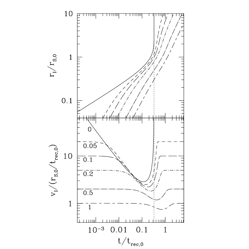
Figure 4: Relativistic I-front radius (upper panel) (in units of Strömgren radius $r_{\rm S,0}$ at central density) and velocity (lower panel) (in units of $r_{\rm S,0}/t_{\rm rec,0}$) along the symmetry axis (z-axis) versus time (in units of central recombination time $t_{\rm rec,0}$) for same plane-stratified case as shown in Figure 3. Each curve is for a different value of $q=r_{\rm S,0}/(ct_{\rm rec,0})$ (as labelled in lower panel), with $q=0$ corresponding to the nonrelativistic solution (solid). In these units, the speed of light is $q^{-1}$. Vertical dotted line marks the finite time $t_{\infty}$ at which the NR solution (q=0) reaches infinite radius: $z_{I}(t_{\infty})=\infty$. All curves assume $Y_{0}=1/2$.

Application of equation (21) to the stratified density profile of equation (52) leads to the following angle-dependent differential equation for the evolution of the I-front radius,

$$\frac{dY_{I}}{dw}=\frac{1-f(Y_{I},\theta)}{3Y_{I}^{2}g(Y_{I},\theta)+q(1-f(Y_{I},\theta))},$$ (55)

where $Y_{I}(\theta)\equiv r_{I}(\theta)/r_{\rm S,0}$, $w\equiv t/t_{\rm rec,0}$,

$$f(Y,\theta)=\frac{0.66Y_{0}^{3}}{\sin^{3}(\theta)}\tanh^{3}\left(\frac{Y\sin(\theta)}{0.88Y_{0}}\right),$$ (56)

and

$$g(Y,\theta)={\rm sech}^{2}\left[Y/Y_{0}\sin(\theta)\right].$$ (57)

In deriving equations (55)-(57), we have measured the polar angle $\theta$ of the direction from the central source to a point on the I-front with respect to the $z=0$ plane, so $\theta=\pi/2$ corresponds to the symmetry axis (i.e. the $z$-axis). We have also followed Franco et al. (1990) in evaluating the recombination integral in equation (21) along each direction by approximating the integral using

$$\int_{0}^{p}p^{2}{\rm sech}^{4}(p)dp\simeq 0.22{\rm tanh}^{3}\left(\frac{p}{0.88}\right),$$ (58)

where $p\equiv(r/z_{0})\sin\theta$.

Illustrative solutions of equations (55)-(57) for relativistic and nonrelativistic I-fronts in a plane-stratified medium are plotted in Figures 3 and 4. We adopt the value $Y_{0}=1/2$ in all cases. Figure 3 shows the two-dimensional, axisymmetric I-front surfaces at different times for the nonrelativistic solution ($q=0$) and for the relativistic solution for $q=1$. The NR I-front solution starts out at superluminal speeds and decelerates in all directions. Along the symmetry axis, the NR I-front eventually reaches a minimum velocity and, thereafter, accelerates upward. This acceleration leads to a superluminal “blow out” in which the NR I-front reaches infinite height in a finite time $t_{\infty}$. In the perpendicular direction, however, along the plane of symmetry at $z=0$, the NR I-front decelerates continuously and approaches the Strömgren radius of a uniform sphere of the same density. The relativistic I-front also starts out decelerating but remains close to the speed of light in all directions, so its shape is initially quite spherical. Like the NR I-front, the relativistic I-front also reaches a minimum speed along the symmetry axis, before it accelerates upward once again and approaches the speed of light. Since its speed is always finite, however, the relativistic I-front cannot “blow-out” as the NR front does in a finite time. Since, in the central plane, the relativistic I-front slows to approach the same Strömgren radius as does the NR solution, above this plane it must balloon upward and outward, confined at the waist by this “Strömgren belt”.

4 Cosmological Relativistic I-fronts

Next we generalize the treatment by Shapiro & Giroux (1987) of an I-front in a uniformly expanding cosmological background at a redshift $z$, to take account of special relativity. Here it is convenient to define the cosmological scale factor as $a=(1+z_{i})/(1+z)$, where $z_{i}$ is the redshift of the source turn-on, corresponding to initial time $t_{i}$. The comoving hydrogen number density ($n_{H,i}$), I-front radius ($r_{I}$), and velocity ($v_{I}$), then correspond to quantities in proper coordinates (in the frame of the source) as $n_{H,p}=n_{H,i}/a^{3}$, $r_{I,p}=ar_{I}$, and $v_{I,p}=dr_{I,p}/dt=d(ar_{I})/dt,$ which means that these comoving quantities are defined at the source turn-on time, not at the present as is often done.

4.1 Relativistic I-front Velocity in the Cosmologically Expanding IGM

For a relativistic I-front in the cosmologically expanding IGM at redshift $z$, the velocities of the front and of the gas just outside it as measured in the lab frame (i.e. the source rest frame) are the proper velocities, $v_{I,p}=\beta_{I,p}c$ and $v_{g,1,p}=\beta_{g,1,p}c$, respectively. This latter gas proper velocity is the sum of the proper Hubble velocity at the location of the front at the proper radius $r_{I,p}$, $v_{h}(r_{I,p})=\beta_{h}(r_{I,p})c$, and its proper peculiar velocity, $v_{g,pec}$,

$$v_{g,1,p}=v_{h}(r_{I,p})+v_{g,pec}$$

$$=H(z)r_{I,p}+v_{g,pec},$$ (59)

where $H(z)$ is the Hubble constant at redshift $z$. We are interested in I-front radii that are small compared with the horizon, so $Hr_{I,p}\ll c$, and in situations in which $v_{g,pec}\ll c$ as well. For the problem of an I-front in the uniformly-expanding, mean IGM, in fact, we can set $v_{g,pec}=0$. The I-front velocity measured by the gas at that location is the proper peculiar velocity $v_{I,pec}^{\prime}$, given by equation (1) as

$$v_{I,pec}^{\prime}=\frac{v_{I,p}-v_{h}(r_{I,p})}{1-\frac{v_{h}(r_{I,p})v_{I,p}}{c^{2}}}=\frac{v_{I,p}-H(z)r_{I,p}}{1-\frac{H(z)r_{I,p}v_{I,p}}{c^{2}}}.$$ (60)

Let us define the proper peculiar velocity of the I-front as measured in the lab frame of the source as $v_{I,pec}=\beta_{I,pec}c$, where

$$v_{I,pec}=v_{I,p}-H(z)r_{I,p}=a\frac{dr_{I}}{dt}.$$ (61)

Equations (60) and (61) then yield

$$v_{I,pec}^{\prime}=\beta_{I,pec}^{\prime}c=\frac{\beta_{I,pec}c}{1-\beta_{h}\beta_{I,p}}.$$ (62)

According to equation (6), the proper peculiar velocity of the I-front in the lab frame of the source is given in terms of these quantities by

$$\beta_{\rm I,pec}=\left[\frac{(1-\beta_{I,p}\beta_{h})}{\gamma_{\rm I,pec}^{\prime}}\right]\left[\frac{\gamma_{I,p}(1-\beta_{I,p})F}{\beta_{i}n_{H,p}c}\right],$$ (63)

where $\beta_{I,p}=\beta_{\rm I,pec}+\beta_{h}$, $\gamma^{\prime}_{\rm I,pec}\equiv\gamma(\beta^{\prime}_{\rm I,pec})$, and we have replaced $n_{H,1}$ by $n_{H,p}\gamma_{h}$ (using equation [7]). Substituting equation (62) into equation (63) yields an equation that can be solved for $\beta_{\rm I,pec}$ as a function of $\beta_{h}$ and the quantity $F/(\beta_{i}n_{H,p}c)$. There are two roots to this equation, corresponding to $\beta_{\rm I,pec}>1$ and $\beta_{\rm I,pec}<1$, respectively. The physical solution must have $\beta_{\rm I,pec}<1$, which yields

$$\beta_{\rm I,pec}=\frac{a}{c}\frac{dr_{I}}{dt}=\frac{(1-\beta_{h})F}{\beta_{i}n_{H,p}\gamma_{h}c+F}.$$ (64)

The photon flux $F$ in equation (64) is that at the location of the I-front as measured in the frame of the source, given by equations (18) and (19) as

$$F(r_{I},t)=\frac{S(r_{I},t_{R})}{4\pi a^{2}r_{I}^{2}},$$ (65)

with

$$S(r_{I},t_{R,I})=\dot{N}_{\gamma}(t_{R,I})-\int_{0}^{ar_{I}}dr_{p}\cdot 4\pi r_{p}^{2}\chi_{\rm eff}x^{2}n_{H,p}^{2}\gamma_{h}^{-2}\alpha_{B}C,$$ (66)

where the proper radius $r_{p}$ is related to the comoving radius $r$ by $r_{p}=ar$, the retarded time is $t_{\rm R,I}=t-r_{\rm I,p}/c$ and the quantities inside the integral are evaluated at the time $t^{\prime}=t_{\rm R,I}+r_{p}/c$.

The Hubble velocities across the H II regions of interest to us here are always much smaller than the speed of light. For a flat universe in the matter-dominated era, with total matter density $\Omega_{0}$ in units of the critical density and Hubble constant $h$ today in units of $100\rm\,km\,s^{-1}Mpc^{-1}$, cosmic expansion results in a Hubble velocity at the proper radius, $r_{\rm I,p}$, of the I-front, given by

$$\beta_{h}(r_{\rm I,p},z)=\frac{H(z)r_{\rm I,p}}{c}\approx 4.54\times 10^{-3}\left(\frac{\Omega_{0}h^{2}}{0.15}\right)^{1/2}\left(\frac{1+z}{7}\right)^{1/2}\left(\frac{r_{I,p}}{6\,{\rm Mpc}}\right).$$ (67)

Since the largest H II regions (e.g. around rare luminous QSOs) are estimated to be several Mpc in proper radius at $z\sim 6$, this implies that $\beta_{h}$ is always less than of order 1%. In that case, we can simplify equations (64)-(66) above by setting $\beta_{h}=0$ and $\gamma_{h}=1$, to yield

$$\beta_{\rm I,pec}=\frac{a}{c}\frac{dr_{I}}{dt}=\frac{F}{\beta_{i}n_{H,p}c+F},$$ (68)

where

$$F=\frac{\dot{N}_{\gamma}(t_{R})-{4\pi}r_{I}^{3}a^{-3}{n_{H,i}}^{2}C\alpha_{B}\chi_{\rm eff}/3}{4\pi a^{2}r_{I}^{2}}.$$ (69)

In terms of the comoving volume , $V_{I}=4\pi r_{I}^{3}/3$, equations (68) and (69) yield

$$\frac{dV_{I}}{dt}=\frac{\dot{N}_{\gamma}(t_{R})-C\alpha_{B}\chi_{\rm eff}n_{H,i}^{2}a^{-3}V_{I}}{\beta_{i}n_{H,i}+\frac{a}{4\pi r_{I}^{2}c}\left[\dot{N}_{\gamma}(t_{R})-C\alpha_{B}\chi_{\rm eff}n_{H,i}^{2}a^{-3}V_{I}\right]}.$$ (70)

Equation (70) can also be derived from the cosmological equivalent of the photon conservation equation (23). This last approach was first proposed (in a simplified form that did not account for recombinations or the presence of helium) by White et al. (2003) (in their Appendix). Equation (70) was previously derived, including the effect of recombinations, but not of helium, by Yu & Lu (2005) using a different approach from ours.

Following the approach in Shapiro & Giroux (1987), we define the dimensionless volume as

$$y\equiv V_{I}/V_{S,i},$$ (71)

where $V_{S,i}$ is the initial Strömgren volume, $V_{S,i}=4\pi r_{S,i}^{3}/3=\dot{N}_{\gamma,i}(\alpha_{B}C\chi_{\rm eff}n^{2}_{H,i})^{-1}$, and the dimensionless time as

$$x\equiv t/t_{i},$$ (72)

which is scaled in terms of the initial time rather than in terms of the recombination time as $w$ was above. Substituting these relations into equation (70), and using the fact that, for the matter-dominated era, $x=a^{3/2}$, we obtain (for $\beta_{i}=\chi_{\rm eff}$)

$$\frac{dy}{dx}=\frac{\lambda[l(x_{R})-y/x^{2}]}{1+(q\chi_{\rm eff}^{-1}/3)(x/y)^{2/3}[l(x_{R})-y/x^{2}]},$$ (73)

where

$$\lambda\equiv\frac{t_{i}}{\chi_{\rm eff}t_{\rm rec,i}}=t_{i}C\alpha_{B}n_{H,i},$$ (74)

is the ratio of the age of the universe to the recombination time when the source turned on, divided by $\chi_{\rm eff}$,

$$q\equiv\frac{r_{S,i}}{ct_{\rm rec,i}}=\frac{r_{S,i}\chi_{\rm eff}\lambda}{ct_{i}},$$ (75)

is the light-crossing time of the initial Strömgren radius, in units of the initial recombination time, and

$$l(x)\equiv\dot{N}_{\gamma}(t)/\dot{N}_{\gamma}(t_{i})\equiv\dot{N}_{\gamma}(x)/\dot{N}_{\gamma,i}$$ (76)

is the ionizing photon luminosity in units of its initial value (i.e. $l(x)\equiv 1$ for a steady source). For $q=0$ ($c\rightarrow\infty$), equation (73) reduces to the nonrelativistic form derived by Shapiro & Giroux (1987), for which they gave an exact analytical solution for the case of a steady source, as follows:

$$y_{\rm NR}(x)={\lambda}e^{\lambda/x}\left[x{\rm Ei}(2,{\lambda}/{x})-{\rm Ei}(2,\lambda)\right],$$ (77)

where ${\rm Ei}(2,x)\equiv\int_{1}^{\infty}\frac{e^{-xt}}{t^{2}}dt$ is the Exponential integral of second order. This exact solution also applies to a flat universe with a cosmological constant in the matter-dominated era (Iliev et al. 2005a). As described in § 3.1, we can use this exact solution of the NR I-front equations to derive the exact solution of the relativistic I-front equations (i.e. arbitrary $q\neq 0$) directly, if we replace the time $t$ in the NR solution by the retarded time $t_{R}$. In that case, the exact, analytical, relativistic I-front solution is given by the following implicit equations:

$$y(x)=y_{\rm NR}(x_{R})={\lambda}e^{\lambda/x_{R}}\left[x_{R}{\rm Ei}(2,{\lambda}/{x_{R}})-{\rm Ei}(2,\lambda)\right],$$ (78)

and

$$x=x_{R}+x^{2/3}y_{\rm NR}^{1/3}(x_{R})\left(\frac{q}{\lambda\chi_{\rm eff}}\right),$$ (79)

where we have used the fact that $a(x)=x^{2/3}$, $x=x_{R}+r_{I,p}(x)/(ct_{i})$, and $r_{I,p}(x)=a(x)r_{S,i}[y_{\rm NR}(x_{R})]^{1/3}$. Equations (78) and (79) easily reduce to a cubic equation for $x(x_{R})$, which has an exact analytical solution with one physical root. Since it is a rather lengthy expression, we omit it here.

For each value of $\lambda,$ we obtain a family of solutions for different values of $q$. In fiducial units

$$\lambda = 0.822C{(1+z_{i})_{10}^{3/2}}\left(\frac{\Omega_{0}h^{2}}{0.15}\right)^{-1/2}\left(\frac{\Omega_{b}h^{2}}{0.022}\right)\left(\frac{\chi_{\rm eff}}{1.08}\right)$$ (80)

$$q = 0.0217\chi^{2/3}_{\rm eff}C^{2/3}\dot{N}_{\gamma,56}^{1/3}(1+z_{i})_{10}^{-1/2}\left(\frac{\Omega_{b}h^{2}}{0.022}\right)^{1/3},$$ (81)

where $(1+z_{i})_{10}\equiv(1+z_{i})/10,$ $\dot{N}_{\gamma,56}\equiv\dot{N}_{\gamma}/(10^{56}\rm\,s^{-1})$, and $\Omega_{b}$ is the mean baryonic density in units of the critical density. The solutions for $\lambda=0.5,1,4,$ and 10 and $q\chi_{\rm eff}^{-2/3}=0,0.1,0.2$ and 0.5 are shown in Figures 5 and 6. The relativistic correction is most significant for small $\lambda$ and large $q$ values, i.e. at later times, stronger sources and little or no clumping of the gas.

Figure 5: Cosmological I-front radius versus time for steady source in the mean IGM, with comoving radius in units of the time-varying, comoving Strömgren radius, $r_{S}(t)=a(t)r_{S}(t_{i})$, and time in units of the age of universe $t_{i}$ at source turn-on. Different curves in each panel correspond to different values of $q=r_{S,i}/(ct_{rec,i})$, with $q=0$ (i.e. nonrelativistic limit, top line) and (from top to bottom) $q=0.1,0.2$ and 0.5. Each panel is for different values of $\lambda\equiv{t_{i}}/{(\chi_{\rm eff}t_{\rm rec,i})}$, as labeled. We have assumed that $\chi_{\rm eff}=1$ for simplicity.

Figure 6: Same as Figure 5 but for the I-front peculiar velocity, instead, where $v_{\rm I,pec}$ is in units of $(r_{S,i}/t_{i})$. The speed of light, $c$, corresponds in these units to $(\chi_{eff}\lambda/q)$. We assume $\chi_{eff}=1$ for simplicity.

This leads to somewhat counterintuitive behavior. For example, increasing the clumping factor increases $q$, and naively, based on equation (73), could be expected to cause a stronger relativistic correction. However, it also increases the value of $\lambda$, which results in a smaller relativistic correction. This is because larger clumping of the gas increases the recombinations in the H II region, which decrease the ionizing flux at the front, slowing it down into the nonrelativistic regime. Below we shall see that infall around the source has a similar effect, increasing the density near the source and rendering the relativistic corrections somewhat weaker than a simple, uniform-density treatment would predict.

As in the case of a spherical I-front in a static medium discussed in §3, the apparent size of a cosmological H II region observed at a given time will depend upon the angle between the line of sight to the source and the line connecting the source to the point we observe on the I-front surface. This difference results from the difference in the light travel times for light received by the observer from different locations on the front. If we were to measure the radius of the H II region transverse to the line of sight at the distance of the source, for example, and interpret this as the proper radius given by the relativistic solution at some time $t$, then the line-of-sight radius on the near-side of the source would be given by the nonrelativistic solution at the same physical time. Hence, the line-of-sight radius will appear to be larger than the transverse radius and will appear to have expanded toward the observer at superluminal speeds. This deviation of the shape of the cosmological H II region from spherical was also discussed by Yu (2005) in the context of the H II regions around QSO’s at redshifts $z>6$ whose spectra show Gunn-Peterson troughs.

5 Cosmological Relativistic I-fronts in Presence of Small-scale Structure and Infall

Figure 7: Cosmological I-front radius in present ($z=0$) comoving units, $r_{c}=r_{I}(1+z_{i})$, versus time (since source turn-on) for a large starburst (left panels) and a luminous QSO (right panels) in the local IGM with infall density profile, both starting at $z_{i}=7$, with assumed parameters as described in the text, for the cases with mean ($C=1$) and clumped ($C=10$) IGM, with and without minihalos present, as labeled, for the relativistic case (solid) and the corresponding nonrelativistic one (dashed).

When self-shielded neutral structures (minihalos) are present on the path of the propagating cosmological I-front, we follow the approach in Iliev et al. (2005a). In this case the I-front jump condition in equation (64) and the I-front evolution equation (70) are modified by setting

$$\beta_{i}\equiv(1-f_{\rm coll})\chi_{\rm eff}+[1+A({\rm He})]f_{\rm coll,MH}\bar{\xi},$$ (82)

where $f_{\rm coll}$ is the total collapsed baryon fraction, $f_{\rm coll,MH}$ is the collapsed fraction of just the minihalos, and $\xi$ is the number of ionizing photons consumed per minihalo atom such that $\bar{\xi}$ is the appropriate average over the distribution of minihalos at the instantaneous location of the global I-front. This photon consumption factor is flux-dependent and in the relativistic case the appropriate flux is $F$, the flux of ionizing photons in the frame of the source, as the relative velocity between the source and the minihalos is much smaller than $c$.

The average number of ionizing photons absorbed per minihalo atom at the current location of the I-front, $\bar{\xi}$, is given by integrating the photon consumption rate $\xi$ per individual minihalo over the Press-Schechter mass function of minihalos at that epoch. The photon consumption rates for individual minihalos were determined by Iliev et al. (2005b) using high-resolution, numerical gas dynamics simulations that included radiative transfer. They have summarized their detailed results by providing fitting formulae for the individual minihalo consumption rates and their dependence on halo mass, redshift, incident flux and ionizing source spectrum. According to Iliev et al. (2005b),

$$\xi(M,z,F_{0})\equiv 1+4.4M_{7}^{0.334+0.023\log_{10}M_{7}}F_{0}^{0.199-0.042{\rm log_{10}}F_{0}}(1+z)_{10},$$ (83)

for a $5\times 10^{4}K$ blackbody external ionizing spectrum, representing Pop. II stars (and similar numbers for a QSO spectrum), for a minihalo of mass $M_{7}$ (in units of $10^{7}M_{\odot}$), overtaken by an intergalactic I-front at a redshift of $z$ which is driven by an external source of flux $F_{0}$, the flux in units of that from a source emitting $10^{56}$ ionizing photons per second at a proper distance $d$ of 1 Mpc, i.e. $F_{0}\equiv{\dot{N}_{\gamma,56}}/{d^{2}_{\rm Mpc}}$. Again, the relevant flux to use in calculating $\xi$ is $F$, the photon flux in the source frame, as it is only the ionization front, not the self-shielded structures, that is moving relativistically with respect to the source. Our model takes account of the biasing of minihalos with respect to the ionizing sources (i.e. the clustering of minihalos in space) by modifying the mass function of the minihalos as a function of their distance from the central source halo in each H II region. It also includes a simple treatment of the effect of local infall on the density of the IGM and the clustering of minihalos surrounding each source [see Iliev et al. (2005a) for details].

In the results below we specialize to a Cold Dark Matter (CDM) cosmological model with parameters $h=0.7$, $\Omega_{0}$ = 0.3, $\Omega_{\Lambda}$ = 0.7, and $\Omega_{b}=0.045$, $\sigma_{8}=0.87$, where $\Omega_{\Lambda}$ is the total vacuum density in units of the critical density, $\sigma_{8}^{2}$ is the variance of linear fluctuations extrapolated to the present and filtered on the $8h^{-1}{\rm Mpc}$ scale, and $n_{p}$ is the index of the power spectrum of primordial density fluctuations (Spergel et al. 2003). Note, however, that as the fronts we are considering are all at high redshifts, the value of $\Omega_{\Lambda}$ has no direct impact on our calculations. Finally, the Eisenstein & Hu (1999) transfer function was used. In Figure 7, we show our results for the I-front radius evolution for two representative sources. The first is a galaxy of total mass $10^{11}M_{\odot}$ at an initial redshift of $z_{i}=7$ (corresponding to a 3-$\sigma$ density fluctuation), which hosts a starburst that produces a total of $f_{\gamma}=250$ ionizing photons per baryon within a lifetime of $t_{s}=3$ Myr, corresponding to $\dot{N}_{\gamma}=4.08\times 10^{55}\rm s^{-1}$. For $t>t_{s}$, the ionizing photon production is assumed to drop as $t^{-4.5}$ (Haiman & Holder 2003). The second source roughly corresponds to a high-redshift luminous QSO, similar to those found by the Sloan Digital Sky Survey (e.g. Fan et al. 2004). Here we assume an ionizing photon production rate of $\dot{N}_{\gamma}=10^{57}\rm s^{-1}$, a source lifetime $t_{s}=30$ Myr starting at $z=7$, and a host halo of $10^{13}M_{\odot}$. For $t>t_{s}$, we model the drop in the ionizing photon production rate as an even steeper power of time, $\dot{N}_{\gamma}(t>t_{s})\propto t^{-10},$ although the precise form of this fall-off is unimportant since we are interested in the expansion phase of the H II region. We show the relativistic results (solid) and the naïve nonrelativistic results (dashed) for direct comparison, and consider four cases with mean ($C=1$) and clumped ($C=10$) IGM, with and without minihalos present.

For both sources, the I-front expansion is initially superluminal in the nonrelativistic model, causing the H II region radius to be significantly larger than the correct, relativistic model. These differences diminish somewhat at later times, but remain significant throughout the expansion phase of the H II region. For both sources, the IGM clumping has only a modest effect, since even for $C=10$ the recombination times are longer than the source lifetimes. The presence of minihalos, on the other hand, decreases the size of the H II regions more considerably, by about 25% in each case. We have also calculated the I-front expansion for a weaker source at higher redshift (a galaxy halo of total mass $10^{8}M_{\odot}$ at initial redshift $z_{i}=15$, corresponding to a $3-\sigma$ density fluctuation, which hosts a Pop. II starburst that produces a total of $f_{\gamma}=250$ ionizing photons per baryon within a lifetime of $t_{s}=3$ Myr) and, as expected from Figure 1, the relativistic correction in this case was negligible.

Finally, we quantified the impact of relativistic effects on the global progress of reionization by recalculating the reionization models described in detail in Iliev et al. (2005a). For all models, the relativistic corrections were small, decreasing the global ionized mass fraction at any given time by $\sim 1\%$ as compared to the nonrelativistic treatment. The corresponding effect on the mean electron-scattering optical depth $\tau$ was even smaller, never exceeding a small fraction of 1%. Thus while the relativistic expansion of an I-front about an individual strong source close to overlap is important, it can generally be ignored when computing the global reionization history, especially given the other significant uncertainties involved.

6 Summary and Conclusions

We have considered the effect of special relativity on the propagation of ionization fronts. The standard (nonrelativistic) treatment of I-fronts neglects the finite speed of light and the relative motion of the radiation source and the gas it ionizes. As a result, when the ionizing photon-to-atom ratio exceeds unity at the location of the I-front, unphysical superluminal I-front motion is predicted to occur. We have generalized the I-front continuity jump condition and the equations that describe the transfer of ionizing radiation between the source and the I-front to take account of these things in a relativistically-correct way. By combining these equations, we have derived the relativistic equation of motion for the R-type I-front created when a point source of ionizing radiation turns on in a neutral gas, including the possibility that the gas is non-uniform and in motion. We then applied this relativistic equation to several illustrative problems of interest in the theory of H II regions in the interstellar and intergalactic media, including the cosmological problem of the reionization of the universe. These include the cases of a steady source in a static gas that is either uniform, spherically-symmetric with a power-law density profile or plane-stratified. We have also solved the problem of a point source in a cosmologically-expanding IGM. We have shown that, in all cases, the radius of the relativistic I-front at a given physical time is identical to that in the nonrelativistic solution in which the physical time $t$ is replaced by the retarded time, equal to $t$ minus the light-travel time from the source to the front.

In the case of a static medium, we obtain an exact analytical solution for the problem of a steady source in a uniform gas, which depends only on the parameter $q$, the time for light to cross the Strömgren radius, in units of the recombination time. Applying this solution to the problem of an O-type star or OB association in a molecular cloud, we find $q$ values of order unity over the full range of appropriate densities and fluxes. However, while this implies that corrections are formally important, they only affect ionization fronts during the rapidly-expanding R-type phase, which lasts only until the I-front expands to fill the Strömgren sphere, and not during the slower D-type hydrodynamic expansion that dominates the bulk of the evolution of these H II regions.

For a source in a nonuniform, static gas, however, I-fronts can, in principle, accelerate back up to relativistic speeds if they propagate down a steep enough density gradient. We have solved this problem for the cases of a power-law density profile in spherical symmetry and a plane-stratified gas. These solutions depend both upon the value of the parameter $q$ calculated at the central density in the core of these nonuniform profiles and on the dimensionless ratio of the core radius of the density profile (or the scale-height in the plane-stratified case) to the Strömgren radius. Such solutions are relevant, for example, to the “champagne phase” of the H II region, which results when the D-type I-front from a stellar source in a dense environment detaches from the shock that leads it during the dynamical expansion phase, and the resulting R-type front runs away towards large radii. In that case, relativistic corrections are important, not only right after the source turns on, but at late times as well.

In the cosmological case, we have derived the exact, analytical solution for the dependence of the relativistic I-front radius on time, by generalizing the solution derived by Shapiro & Giroux (1987). We find a complete family of solutions that are described by two dimensionless parameters: $q$, which is now defined as the light crossing time at the Strömgren radius in units of the initial recombination time, and $\lambda$, the age of the universe at source turn-on in units of the initial recombination time. In this case, relativistic effects are again important only if $q\mathrel{\hbox{\hbox to0.0pt{\hbox{\lower 4.0pt\hbox{$\sim$}}\hss}\hbox{$>$}}}0.1$ , but now only if $\lambda\mathrel{\hbox{\hbox to0.0pt{\hbox{\lower 4.0pt\hbox{$\sim$}}\hss}\hbox{$<$}}}1$ as well. Thus relativistic corrections are significant only in cases in which both the source flux is large (corresponding to a large $q$) and the redshift is relatively low (corresponding to a small $\lambda$).

Incorporating relativistic effects into the more exact modeling described in Iliev et al. (2005a) allows us to assess the importance of relativistic effects in a realistic reionization scenario that includes both infall and the impact of small-scale (self-shielding) structures. In the individual case of a large galaxy or luminous QSO at the end of the reionization epoch ($z\sim 7$), relativistic effects can be quite significant: resulting in $\approx 4$ and 2 times smaller ionized volumes after 1 and 3 Myrs, respectively, in the galactic case, and $\approx 20$ and 2 times smaller volumes after 1 and 10 Myrs, respectively, in the QSO case. The relative differences then decrease with time, but remain significant until the source luminosity decays. Afterwards, at time $t\sim 2t_{s}$, the relativistic solution for the H II region radius finally matches the nonrelativistic one. Although the I-front propagation becomes subluminal earlier than this, and thus the usual nonrelativistic expression for its speed becomes correct, the radius of the H II region remains smaller throughout the source lifetime. Furthermore, the presence of small-scale structure can decrease the size of the H II region by up to an additional $\sim 25$%.

Generalizing these results to the issue of global reionization, however, yields far less dramatic changes. As most of the intergalactic medium was ionized by smaller (lower $q$) and higher-redshift (higher $\lambda$) sources, we find that relativistic corrections change the ionized mass fraction at any give time by $\sim 1$% with respect to a nonrelativistic approach, and relativistic corrections to the mean electron-scattering optical depth are even smaller. Thus I-fronts, while an intrinsically relativistic phenomenon, can be accurately treated nonrelativistically in studies of global cosmological reionization, but not for the isolated H II regions of short-lived luminous sources at late times, close to the epoch of overlap.

Finally, we note that the original nonrelativistic, cosmological I-front solutions of Shapiro & Giroux (1987) correctly relate the observed line-of-sight distance of the I-front from the source which created it to the source luminosity and IGM neutral density, even for cases in which those nonrelativistic solutions yield a superluminal expansion speed. Thus, the interpretation of the line-of-sight apparent sizes of the cosmological H II regions recently observed in the IGM surrounding high-redshift sources like the SDSS quasars at $z\geq 6$ does not require the relativistic correction described here. This somewhat surprising result was noted previously by White et al. (2003) and others (e.g. Yu & Lu 2005). Our results help to illuminate the connection between the nonrelativistic and relativistic treatments, however, and distinguish the circumstances under which the relativistic corrections do make a difference. For example, when we observe a distant source and match the apparent size of its H II region along the line of sight to the nonrelativistic solution evaluated at some time $t$ (as measured from the source turn-on time), the apparent transverse size at the distance of the source will then be given by the relativistic solution evaluated at this same time $t$.

References

- Bruscoli et al. (2002) Bruscoli, M., Ferrara, A., & Scannapieco, E. 2002, MNRAS, 330, L43
- Churchwell (2002) Churchwell, E. 2002, ARA&A, 40, 27
- Ciardi et al. (2000) Ciardi, B., Ferrara, A., Governato, F., & Jenkins, A. 2000, MNRAS, 314, 611
- Ciardi et al. (2003) Ciardi, B., Stoehr, F., & White, S. D. M. 2003, MNRAS, 343, 1101
- Eisenstein & Hu (1999) Eisenstein, D. J. & Hu, W. 1999, ApJ, 511, 5
- Evans (1999) Evans, N. J. 1999, ARA&A, 37, 311
- Fan et al. (2004) Fan, X., et al. 2004, AJ, 128, 515
- Franco et al. (1990) Franco, J., Tenorio-Tagle, G., & Bodenheimer, P. 1990, ApJ, 349, 126
- Furlanetto et al. (2004) Furlanetto, S. R., Zaldarriaga, M., & Hernquist, L. 2004, ApJ, 613, 1
- Garay & Lizano (1999) Garay, G. & Lizano, S. 1999, PASP, 111, 1049
- Gnedin (2000) Gnedin, N. Y. 2000, ApJ, 535, 530
- Haiman (2002) Haiman, Z. 2002, ApJ, 576, L1
- Haiman & Holder (2003) Haiman, Z. & Holder, G. P. 2003, ApJ, 595, 1
- Hosokawa & Inutsuka (2005) Hosokawa, T. & Inutsuka, S. 2005, ApJ, 623, 917
- Iliev et al. (2005a) Iliev, I. T., Scannapieco, E., & Shapiro, P. R. 2005a, ApJ, 624, 491
- Iliev & Shapiro (2001) Iliev, I. T. & Shapiro, P. R. 2001, MNRAS, 325, 468
- Iliev et al. (2005b) Iliev, I. T., Shapiro, P. R., & Raga, A. C. 2005b, MNRAS, 361, 405
- Kogut et al. (2003) Kogut, A., et al. 2003, ApJS, 148, 161
- Lebrón et al. (2001) Lebrón, M. E., Rodríguez, L. F., & Lizano, S. 2001, ApJ, 560, 806
- Lee et al. (2005) Lee, H., Chen, W. P., Zhang, Z., & Hu, J. 2005, ApJ, 624, 808
- Lefloch et al. (1997) Lefloch, B., Lazareff, B., & Castets, A. 1997, A&A, 324, 249
- Malhotra & Rhoads (2004) Malhotra, S. & Rhoads, J. E. 2004, ApJ, 617, L5
- Mathews & O’Dell (1969) Mathews, W. G. & O’Dell, C. R. 1969, ARA&A, 7, 67
- Oh & Furlanetto (2005) Oh, S. P. & Furlanetto, S. R. 2005, ApJ, 620, L9
- Ricotti et al. (2002) Ricotti, M., Gnedin, N. Y., & Shull, J. M. 2002, ApJ, 575, 49
- Santos (2004) Santos, M. R. 2004, MNRAS, 349, 1137
- Shapiro & Giroux (1987) Shapiro, P. R. & Giroux, M. L. 1987, ApJ, 321, L107
- Shapiro et al. (1999) Shapiro, P. R., Iliev, I. T., & Raga, A. C. 1999, MNRAS, 307, 203
- Shapiro et al. (2004) —. 2004, MNRAS, 348, 753
- Shapiro et al. (1986) Shapiro, P. R., Milgrom, M., & Rees, M. J. 1986, ApJS, 60, 393
- Sokasian et al. (2003) Sokasian, A., Abel, T., Hernquist, L., & Springel, V. 2003, MNRAS, 344, 607
- Spergel et al. (2003) Spergel, D. N., et al. 2003, ApJS, 148, 175
- Stern et al. (2005) Stern, D., et al. 2005, ApJ, 619, 12
- White et al. (2003) White, R. L., Becker, R. H., Fan, X., & Strauss, M. A. 2003, AJ, 126, 1
- Wyithe & Loeb (2003) Wyithe, J. S. B. & Loeb, A. 2003, ApJ, 586, 693
- Wyithe & Loeb (2004) —. 2004, Nature, 432, 194
- Yu (2005) Yu, Q. 2005, ApJ, 623, 683
- Yu & Lu (2005) Yu, Q. & Lu, Y. 2005, ApJ, 620, 31