The Milky Way’s stellar halo - lumpy or triaxial?

Abstract

We present minimum chi-squared fits of power law and Hernquist density profiles to F-turnoff stars in eight 2.5^∘ wide stripes of SDSS data: five in the North Galactic Cap and three in the South Galactic cap. Portions of the stellar Galactic halo that are known to contain large streams of tidal debris or other lumpy structure, or that may include significant contamination from the thick disk, are avoided. The data strongly favor a model that is not symmetric about the Galaxy’s axis of rotation. If included as a free parameter, the best fit to the center of the spheroid is surprisingly $\approx 3$kpc from the Galactic center in the direction of the Sun’s motion. The model fits favor a low value of the density of halo stars at the solar position. The alternative to a non-axisymmetric stellar distribution is that our fits are contaminated by previously unidentified lumpy substructure.

1 Introduction

The stars in the Milky Way are divided into: an old, metal-rich bulge population near the Galactic center; a thin disk population in the plane of the Milky Way that includes a range of stellar ages and metallicities but is unique in including a young, metal-rich population; a thick disk population of intermediate age and metallicity (fraction of elements heavier than helium); and an old, metal-poor spheroid (also called the stellar halo) population in which the disks are embedded. Each of the populations has a distinct kinematic signature. The spheroid is generally described as a somewhat spherical population with a density that falls off as $r^{-\alpha}$, $\alpha=3.5$, where $r$ is the distance from the center of the Galaxy. A squashing parameter $0.5<q<1.0$, in the direction perpendicular to the Galactic plane is also fit to the density distribution of the spheroid by redefining the distance from the Galactic center as: $r=\sqrt{X^{2}+Y^{2}+(Z/q)^{2}}.$

The Sloan Digital Sky Survey (SDSS) scans the sky in $2^{\circ}.5$ wide stripes that follow great circles on the sky. The photometric images are taken in five optical filters: $ugriz$. Data that has been corrected for interstellar reddening using IRAS dust maps [1] is designated by a subscripted zero. Three public data releases [2, 3, 4] are available though an online catalog archive server. Though the survey geometry and technical design [5, 6, 7, 8, 9, 10, 11] optimized extragalactic research, studies of the Galactic stars in the photometric catalog have significantly advanced our knowledge of the stars in the halo of our own Galaxy.

In particular, it has been shown [12] that the distribution of faint F-turnoff stars ($19<g<21.5$) that we generally associate with the spheroid population [13, 14] are not distributed symmetrically about the Galaxy center. Even if regions surrounding known or suspected tidal streams and debris are eliminated from consideration, the stellar distribution is not symmetric about a plane (perpendicular to the Galactic plane) through Galactic longitudes $l=0^{\circ},l=180^{\circ}$. Since there are no values of the axisymmetric power law model parameters ($\alpha,q$) which describe an asymmetric distribution, the standard model must be modified to include asymmetric stellar populations, large scale lumpiness, or an asymmetric smooth spheroid component.

In this paper, we make the assumption that there exists a smooth component to the Galactic halo, and present several candidate models. We then use a minimum $\chi^{2}$ technique to find the best fit parameters for each model, fitting to eight $2^{\circ}.5$ wide stripes of data in the SDSS DR3. These stripes are chosen to sample the widest range of positions available in the Galaxy from this dataset. Figure 1 shows the positions of these data stripes in Galactic coordinates.

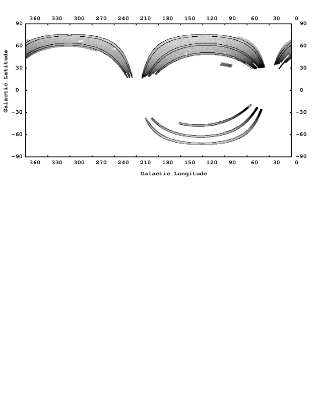
Figure 1: Location of the DR3 data used to fit the spheroid in Galactic coordinates. The grey scale shows spheroid stars selected from DR3 in the manner described in [12]. The black lines show the outlines of eight stripes used in this paper to fit the spheroid models. The SDSS stripes numbered are sequentially in a clockwise direction around the coordinate $(l,b)=(209^{\circ},-7^{\circ})$. This figure shows stripes 10 (bottom) and 15 (top) in the range $0^{\circ}<l<29^{\circ},209^{\circ}<l<360^{\circ}$; and stripes 24, 32, 37, 76, 82, 86, top to bottom, in the range $29^{\circ}<l<209^{\circ}$.

2 Spheroid Models and Parameters

The simplest extension to the oblate power law spheroid model that allows for asymmetry about the Galactic center is a triaxial power law spheroid. In addition to flattening the spheroid by a factor of $q$ in the $Z$ direction, we flatten by a factor of p in the $Y$ direction. This density function with ellipsoidal contours can in general be shifted in three coordinates and rotated by three angles with respect to the Galactic coordinates $(X,Y,Z)$, where $X$ goes from the solar position through the center of the Galaxy, $Y$ is in the direction of the local standard of rest (roughly the direction the Sun is going), and we have a right-handed coordinate system centered on the center of the Milky Way. The principle axes of the density function are:

$$\begin{array}[]{l}X^{\prime}=x\cos\theta\cos\phi+y\sin\theta\cos\phi+z\sin\phi\\ Y^{\prime}=x(-\sin\theta\cos\xi-\cos\theta\sin\phi\sin\xi)+y(\cos\theta\cos\xi-\sin\theta\sin\phi\sin\xi)+z\cos\phi\sin\xi\\ Z^{\prime}=x(\sin\theta\sin\xi-\cos\theta\sin\phi\cos\xi)+y(-\cos\theta\sin\xi-\sin\theta\sin\phi\cos\xi)+z\cos\phi\cos\xi,\\ \end{array}$$

where $x=X-dX,y=Y-dY,$ and $z=Z-dZ.$ Initially, we expected that $dX=dY=dZ=\phi=\xi=0$, but the addition of these parameters to the models significantly improved the fits.

We also found that power laws tended to predict too high a star density near the center of the Galaxy, compared to our data. We achieved a better fit to the data with a Hernquist profile:

$$\rho=\frac{\rho_{0}}{r(r+R_{core})^{3}},r=\sqrt{X^{\prime 2}+(Y^{\prime}/p)^{2}+(Z^{\prime}/q)^{2}}.$$

Although we did explore the possibility of fitting a function of the form:

$$\rho=\frac{\rho_{0}}{r^{\alpha}(r+R_{core})^{\delta}},$$

which would include both the power law model ($\delta=0$) and the Hernquist model ($\alpha=1,\delta=3$), this fitting was abandoned because we are not very sensitive to the combination of $\alpha$ and $\delta$. In general, models with $\alpha+\delta\approx 4$ worked well.

3 F Turnoff Star data

The data includes all stellar objects in the 8 SDSS stripes with: $(r-i)_{0}<0.8$ (to get rid of M stars at faint magnitudes), $0.4<(u-g)_{0}<3.8$ (to eliminate QSOs), $0.0<(g-r)_{0}<0.3$ (to select stars with turnoff colors), and $g_{0}<24.$ The designation as “star” in the database removes issues of duplication of objects due to overlaps and deblending. Objects are further rejected if flags indicate that they are saturated, too near the edge of an image to give good photometry, or classified as a “bright” object. This resulted in selection of (234,306; 190,221; 159,632; 132,637; 123,359; 115,416; 165,620; 150,562) stars from stripes (10, 15, 24, 32, 37, 76, 82, 86), respectively. These stripes are shown in figure 1.

In order to compare the stellar density to the model density for a given set of parameters, the stellar data was sorted into bins that were 0.1 mag. wide in $g_{0}$ and $1^{\circ}$ in angle along the length of the stripe. For a given model, the expected number of stars in each bin was calculated as:

$$N=\rho(r)dV=\rho(r)R^{3}\frac{\ln{10}\Omega dm}{5},$$

where $R$ is the distance from the Sun, $dm$ is the magnitude bin size, $\Omega$ is the solid angle of each bin (2.5 sq. deg.), and $\rho$ is the density of our sample of F turnoff stars.

Since our models included only stars in a smooth spheroid population, we selected data only from parts of sky and magnitude ranges we thought were most likely to contain exclusively stars from this population. Figures 2, 3, 4, 5, 6, 7, 8, and 9 show the outlines of the portions of the data that seemed the most likely to contain purely spheroid stars. Bright magnitudes were avoided, particularly near the Galactic plane, since they could be contaminated with thick disk stars (as determined by Besancon galaxy models [13]). Stars near any previously identified spheroid overdensity were also avoided.

The models were then modified to reflect the uncertainty in the absolute magnitudes of the turnoff stars, which leads to an uncertainty in the distance to each star. We analyzed the stars in the three globular clusters Pal 5 (stripe 10), M15 (stripe 76), and M2 (stripe 82) to determine the turnoff star counts as a function of apparent magnitude. A histogram of star counts vs. $g_{0}$ magnitude was created by subtracting the star counts in a neighboring piece of sky from the star counts in the direction of the globular cluster. A function of the form:

$$f(g_{0})=Ae^{-(g_{0}-g_{peak})/(2\sigma^{2})}\left\{\begin{array}[]{ll}\sigma=0.55,&g_{0}<g_{peak}\\ \sigma=0.75,&g_{0}>g_{peak}\end{array}\right.$$

was a reasonable fit to the data. This is an approximate fit; each of the clusters had a slightly different magnitude profile.

So that the model took into account this range of absolute magnitudes, we convolved the model with this magnitude distribution, adjusting the amplitude $A$ so that the sum of the bins in the convolution kernel was 1.0. This way, the overall normalization of the model was not affected.

4 Minimum $\chi^{2}$ fits

Once a set of data was extracted and a set of models was defined, we fit the models to the data by adjusting the model parameters to produce the minimum $\chi^{2}$. We considered five models: a triaxial Hernquist model in which the center was not fixed to the center of the Galaxy, a triaxial Hernquist model in which the center was forced to the center of the Galaxy, a triaxial power law model in which the center was allowed to float, a triaxial power law model in which the center was forced to the center of the Galaxy, and a traditional axisymmetric power law model. The models contained between 4 and 10 free parameters, depending on the model.

For each model, we chose a starting set of parameters, excluding the normalization $\rho_{0}$, and generated the expected star counts for each bin in the star count data. We then normalized the model so that the sum of all of the star counts equaled the sum of all of the star counts in the data set (including all stripes) that we were fitting. This had the advantage of reducing by one the number of parameters that were allowed to freely vary, since this one could be computed in a straightforward manner. The value of $\chi^{2}$ for this model and this parameter set is then:

$$\chi^{2}=\frac{\sum_{i=0}^{N_{bin}}(d_{i}-m_{i})^{2}/m_{i}}{N_{bin}-N_{param}-2},$$

where $N_{bin}$ is the number of bins used in all stripes, $d_{i}$ represents each bin of the data, $m_{i}$ represents the expected number of counts in that bin in the model, and $N_{param}$ is the number of parameters fit in the model. We have assumed that the statistical errors, $\sigma_{i}$, in the number of stars in the bins are Poisson so that $\sigma_{i}^{2}=m_{i}$.

We changed the parameters in each model by hand until we achieved the minimum $\chi^{2}$ for each model. The final parameters were checked to guarantee that the fit is worse if any of the parameters are changed by $\pm$ the tolerance (given in column 2 of table 1) for that parameter. If there are 10 adjustable parameters, then $3^{10}$ parameter sets were checked to ensure a minimum.

The best fit model parameters are given in table 1. Parameters include: $R_{0}$, distance from the Sun to the Galactic center; $(p,q)$, the ratio of the scale length in the $(Y^{\prime},Z^{\prime})$ directions compared to the major axis in the $X^{\prime}$ direction; $R_{core}$, the Hernquist core radius; $M_{f}$, the peak of the absolute magnitude distribution of our turnoff stars; and $\rho_{0}$, the normalization of the Hernquist or power law model. $(\alpha,\delta)$ are $(1,3)$ for a Hernquist profile and $(\alpha,0)$ for a power law profile. To get from Galactic XYZ coordinates to the principle axes of the triaxial models, we first shift the center by $(dX,dY,dZ)$, then rotate by $\theta$ around the $Z$-axis, then rotate by $\phi$ around the new $Y$-axis, and then by $\xi$ around the new $X$-axis. $N_{solar}$ is the density of the selected turnoff stars in the solar neighborhood and $\chi^{2}$, a measure of the goodness of the model fit.

Numbers in bold were set to a fixed value and were not allowed to vary. Parameters were fixed either because the definition of the model required it (for example, power laws all have $\delta=0$), or because the parameter was correlated with a parameter that was varied. For instance, in the full Hernquist model we set the scale of the model with $R_{core}$, though we could instead have varied $M_{f}$. $R_{0}$ and $dX$ are redundant.

Table 1: Best Fit parameters for five spheroid models described in Section 2. Numbers in bold were fixed; all others were varied to minimize $\chi^{2}$ fit between the model and the data The units of $\rho_{0}$ are kpc⁴ for Hernquist models, and kpc^α for power law models.

	Tol.	Full	Galactocentric	Full	Galactocentric	Standard
		Hernquist	Hernquist	Power Law	Power Law	Power Law
$R_{0}$	0.1 kpc	8.0 kpc	8.5 kpc	8.0 kpc	8.5 kpc	10.7 kpc
$p$	0.01	0.73	0.73	0.74	0.72	1.0
$q$	0.01	0.67	0.60	0.66	0.59	0.63
$\theta$	1∘	48∘	70∘	52∘	72∘	–
$R_{core}$	0.5 kpc	15.0 kpc	14.0 kpc	–	–	–
$dX$	0.1 kpc	0.1 kpc	–	0.2 kpc	–	–
$dY$	0.1 kpc	3.5 kpc	–	3.0 kpc	–	–
$dZ$	0.1 kpc	0.1 kpc	–	0.0 kpc	–	–
$\phi$	0.5∘	-8.0∘	-4.5∘	-6.5∘	-4.0∘	–
$\xi$	2∘	12∘	14∘	16∘	14∘	–
$\alpha$	0.1	1	1	2.9	3.0	3.1
$\delta$	–	3	3	0	0	0
$M_{f}$	0.1	4.2	4.2	4.2	4.2	4.2
$\rho_{0}$		$1.548\times 10^{8}$	$2.093\times 10^{8}$	$1.065\times 10^{6}$	$2.157\times 10^{6}$	$2.390\times 10^{6}$
$N_{solar}$		1081 kpc-3	1096 kpc-3	1412 kpc-3	1341 kpc-3	1539 kpc-3
$\chi^{2}$		1.37	1.42	1.49	1.51	1.92

Figures 2, 3, 4, 5, 6, 7, 8, and 9 show the star density in the data and the residual star densities in each stripe of data after the model has been subtracted. Figure 2 additionally shows the star density of the model for comparison.

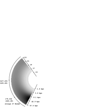
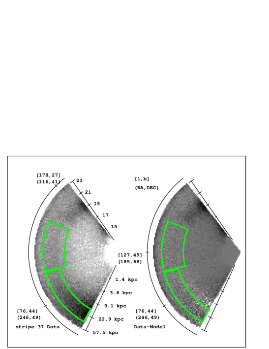
Figure 2: Stripe 37 model, data, and subtraction. The radial coordinate is the reddening corrected $g_{0}$ magnitude; if we assume the turnoff stars all have $M_{g_{0}}=4.2$, then the radial coordinate is logarithmically proportional to distance from the Sun. The approximate distances in kpc are given on the bottom half of the model and data plots. The model and the data are shown with the same grey scale. The two outlined regions on the data and the subtractions show the portions of the data on this stripe that were used to fit the model. We avoided the faintest stars because they might not be complete, the brightest stars because they could be contaminated by thick disk stars, and the portion of the data at the top of the diagram that includes a known overdensity in the Galactic plane [14]. The scale for the model and data is such that zero counts is white; in the subtraction zero counts is grey so that negative deviations (white) and positive deviations (black) are both discernable.

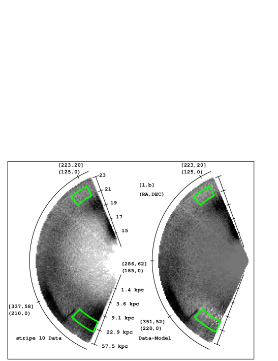
Figure 3: Stripe 10 data and subtraction. Very little of this stripe could be used for comparison due to the tidal stream in the plane near the top of the stripe, the Sagittarius stream on the bottom left, and an apparent overdensity of unknown origin on the middle left. The outlined region on the top of the stripe was included because some of the model fits tended to oversubtract this region.

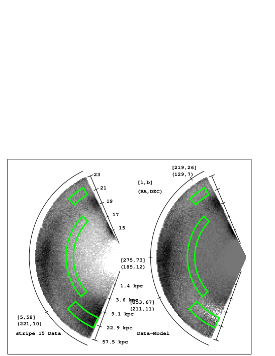
Figure 4: Stripe 15 data and subtraction. Prominent again in this figure are the Sagittarius dwarf tidal stream (left) and a tidal stream in the Galactic plane (top). The excess counts in the subtraction near the bottom of the wedge, near the Galactic center, could include stars leaking into the sample from the thick disk.

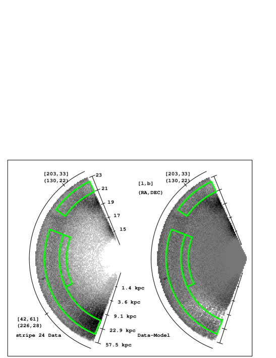
Figure 5: Stripe 24 data and subtraction. This stripe has fewer large tidal streams. The stream in the Galactic plane is still present at the top of the diagram, and there is a small overdensity of unknown origin about $30^{\circ}$ away in the counterclockwise direction. Again, brighter stars near the Galactic center were avoided in the fitting procedure due to possible contamination from the thick disk.

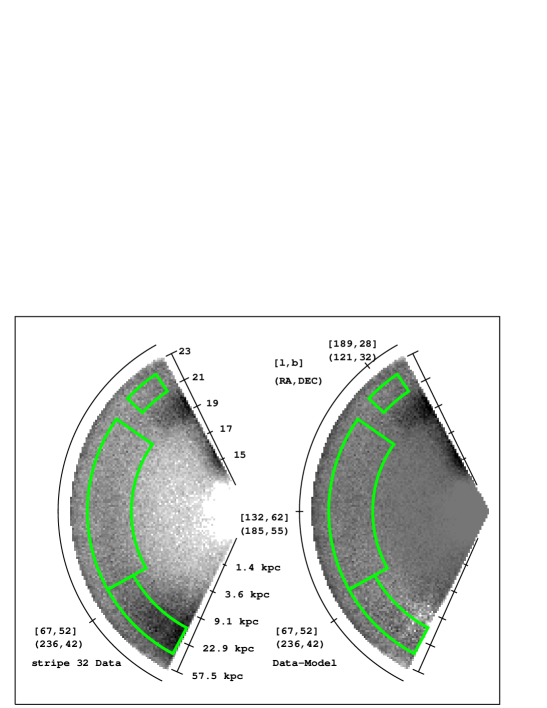
Figure 6: Stripe 32 data and subtraction. This is a very clean stripe, with a nice subtraction. The stream in the plane of the Milky Way is present at the top of the figure.

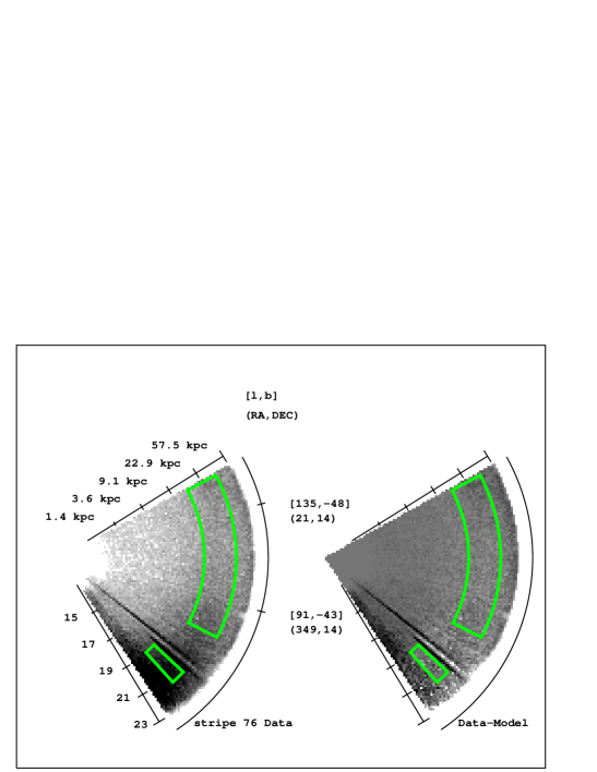
Figure 7: Stripe 76 data and subtraction. This is a shorter section of data that is free from tidal debris, but contains a section of poor data and a globular cluster (M15) that appear as dark radial features.

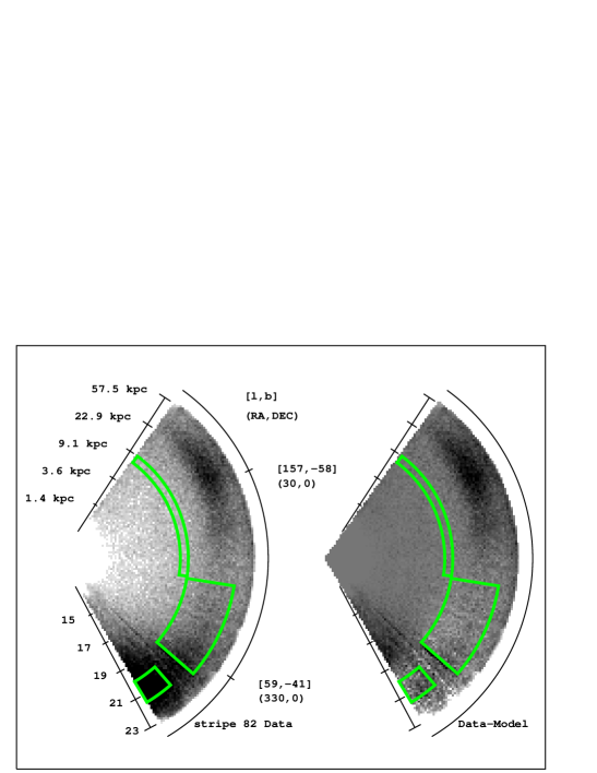
Figure 8: Stripe 82 data and subtraction. The trailing tail of the Sagittarius tidal stream is prominent here. Also, there is a section of poor data and a globular cluster (M2) that show up as radial features most easily seen in the subtraction. The poor subtraction near the Galactic center (bottom) at bright magnitudes could be due to thick disk stars leaking into the sample.

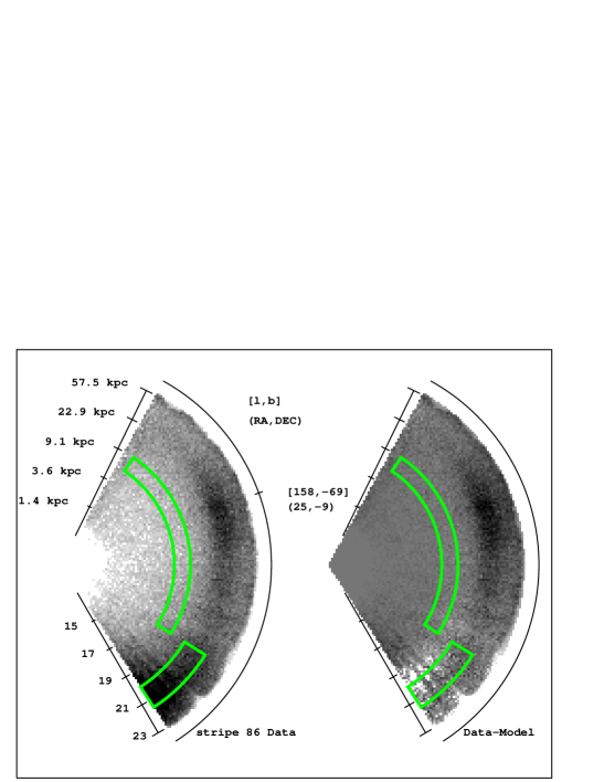
Figure 9: Stripe 86 data and subtraction. The Sagittarius stream trailing tidal tail is also prominent in this stripe. The data near the Galactic center shows a radial pattern that is indicative of poorer photometric data. We experimented with leaving this stripe in and taking it out. In the end we decided to keep the data since the fits to this stripe were fairly consistent with the other southern stripes, and keeping it improved the overall appearance of the subtractions.

A crude estimate for the mass density of stars in the solar neighborhood is calculated from SDSS measurements of the Pal 5 globular cluster. There are 588 stars above background with $0.0<g_{0}-r_{0}<0.3$ in Pal 5. The mass of Pal 5 is 4.5 to $6.0\times 10^{3}{\rm M}_{\odot}$ [15]. Assuming that Pal 5 is a good approximation to the stellar population of the spheroid (a big assumption), an estimate of the number of solar masses per sample star is $10{\rm M}_{\odot}/$star. Therefore, the local mass density of the stellar spheroid is 11,000 M${}_{\odot}/$kpc³ for the full Hernquist model, and 15,000 M${}_{\odot}/$kpc³ for the best fit standard power law. These numbers are 20-25 times lower than the average density from Allen’s Astrophysical Quantities [16] of $2.6\times 10^{5}{\rm M}_{\odot}/{\rm kpc}^{3}$. Since Pal 5 has a bluer turnoff than the spheroid, it is likely that using this cluster to estimate the mass of the spheroid component leads to an underestimate, though it seems unlikely that it could account for the whole difference. Future work will provide a better estimate of the spheroid normalization.

5 Conclusions

The standard stellar density profile used to fit the Galactic spheroid, $\rho=\rho_{0}/r^{\alpha},$ is an extremely poor fit to the density of halo turnoff stars when a large area of the sky is sampled, even using the unusually large best fit distance between the Sun and the Galactic center. The flattening of $q=0.63$ and the power law slope of $\alpha=3.1$ are within the range of previously measured values.

Triaxial models are best fit with a major axis $50-70^{\circ}$ from the line of sight from the Sun to the center of the Galaxy and tilted $4^{\circ}-6^{\circ}$ from the Galactic plane. The minor axis, $\approx 13^{\circ}$ from the $Z$-direction, is about $65\%$ of the scale length of the major axis. The intermediate axis is about $75\%$ of the scale length of the major axis, and tilted at about $12^{\circ}$ from the Galactic plane. These models are clearly favored over the axisymmetric standard model.

The Hernquist profile is a better fit to the data than a power law profile, but give roughly similar values for the positional and flattening parameters. All of the models suggest a lower spheroid stellar density near the Sun compared with previous estimates.

If the center of the spheroid profile is allowed to vary, then it moves a surprising 3.0 - 3.5 kpc from the nominal center of the disk in the direction of the Sun’s motion. Since this is perpendicular to the line of sight from the Sun to the Galactic center, it is not possible to reduce this offset by simply changing the scale lengths or assumed absolute magnitudes of the sample stars. It is the stars in the southern stripes near the Galactic center that tend to pull the spheroid density off center. We are still investigating whether there could be unidentified substructure or data quality issues at the root of this surprising result. Clearly, more data in the southern hemisphere would be useful in understanding the large-scale distribution of stars in the halo.

A large fraction of the Galactic halo contains known substructure that must be avoided to fit the smooth component. It is unknown whether the results provided here are contaminated by unidentified substructure.

H. J. N. acknowledges funding from Research Corporation and the National Science Foundation (AST 03-07571). Ken Freeman and Markus Samland provided stimulating discussion of the of the stellar content of the Milky Way.

Funding for the creation and distribution of the SDSS Archive has been provided by the Alfred P. Sloan Foundation, the Participating Institutions, the National Aeronautics and Space Administration, the National Science Foundation, the U.S. Department of Energy, the Japanese Monbukagakusho, and the Max Planck Society. The SDSS Web site is http://www.sdss.org/.

The SDSS is managed by the Astrophysical Research Consortium (ARC) for the Participating Institutions. The Participating Institutions are The University of Chicago, Fermilab, the Institute for Advanced Study, the Japan Participation Group, The Johns Hopkins University, the Korean Scientist Group, Los Alamos National Laboratory, the Max-Planck-Institute for Astronomy (MPIA), the Max-Planck-Institute for Astrophysics (MPA), New Mexico State University, University of Pittsburgh, University of Portsmouth, Princeton University, the United States Naval Observatory, and the University of Washington.

References

- [1] Schlegel D J, Finkbeiner D P and Davis M 1998 Astrop. J. 500 525
- [2] Abazajian K et al. 2003 Astron. J. 126 2081
- [3] Abazajian K et al. 2004 Astron. J. 128 502
- [4] Abazajian K et al. 2005 Astron. J. 129 1755
- [5] Fukugita M, Ichikawa T, Gunn J E, Doi M, Shimasaku K and Schneider D P 1996, Astron. J. 111 1748
- [6] Gunn J E et al. 1998 Astron. J. 116 3040
- [7] Hogg D W, Finkbeiner D P, Schlegel D J and Gunn J E 2001, Astron. J. 122 2129
- [8] Stoughton C et al. 2002 Astron. J. 123 485
- [9] Pier J R, Munn J A, Hindsley R B, Hennessy G S, Kent S M, Lupton R H and Ivezic Z 2003 Astron. J. 125 1559
- [10] Smith J A et al. 2002 Astron. J. 123 2121
- [11] York D G et al. 2000 Astron. J. 120 1579
- [12] Newberg H J and Yanny B 2005 Astrometry in the Age of the Next Generation of Large Telescopes (18-20 October 2004, Flagstaff, AZ) vol 338 ed A K B Monet and K Seidelmann (San Francisco: PASP Conf. Ser.) in press (Preprint astro-ph/0502386)
- [13] Robin A C, Reyle S D and Picaud S 2003 Astron. Astrophys. 409 523
- [14] Newberg, H J et al. 2002 Astroph. J. 569 245
- [15] Odenkirchen M, Grebel E K, Dehnen W, Rix H-W and Cudworth K M 2002 Astron. J. 124 1497
- [16] Cox A 1999 Allen’s Astrophysical Quantities fourth edition (New York: Springer-Verlag) chapter 23 p 571