Neutrino-driven convection versus advection in core collapse supernovae

Abstract

A toy model is analyzed in order to evaluate the linear stability of the gain region immediately behind a stalled accretion shock, after core bounce. This model demonstrates that a negative entropy gradient is not sufficient to warrant linear instability. The stability criterion is governed by the ratio $\chi$ of the advection time through the gain region divided by the local timescale of buoyancy. The gain region is linearly stable if $\chi<3$. The classical convective instability is recovered in the limit $\chi\gg 3$. For $\chi>3$, perturbations are unstable in a limited range of horizontal wavelengths centered around twice the vertical size $H$ of the gain region. The threshold horizontal wavenumbers $k_{\rm min}$ and $k_{\rm max}$ follow simple scaling laws such that $Hk_{\rm min}\propto 1/{\chi}$ and $Hk_{\rm max}\propto\chi$. The convective stability of the $l=1$ mode in spherical accretion is discussed, in relation with the asymmetric explosion of core collapse supernovae. The advective stabilization of long wavelength perturbations weakens the possible influence of convection alone on a global $l=1$ mode.

1 Introduction

Convective instabilities may be an important ingredient of the explosion mechanism of core collapse supernovae. Below the neutrinosphere, they can increase the neutrino luminosity, and in the neutrino heating layer they can help pushing the shock farther out. Convection in the supernova core may also be the seed for the large-scale anisotropies seen in many supernovae and supernova remnants and might be linked to the measured high velocities of young pulsars (e.g., Arnett 1987, Woosley 1987, Herant et al. 1992). Negative gradients of entropy were initially thought to arise as a natural consequence of the decline of the shock strength due to photodissociation of heavy nuclei and neutrino escape (Arnett 1987, Burrows 1987, Bethe, Brown & Cooperstein 1987, Bethe 1990). A more durable effect was recognized by Herant, Benz & Colgate (1992) in their simulations: neutrino heating is able to maintain a negative entropy gradient in a “gain region” immediately behind the stalled shock. They also observed that the convective eddies tend to merge and produce eddies of the size of the computing box. Similar results were found in the numerical simulations of Herant et al. (1994), Burrows et al. (1995), Janka & Müller (1996), Mezzacappa et al. (1998).

Are such convective instabilities able to produce an $l=1$ asymmetry as suggested by Herant (1995) and Thompson (2000) and seen more recently in numerical simulations (Scheck et al. 2004)? Estimates of the linear growth rate and wavelength of the nonspherical modes found in these studies cannot be directly made on grounds of the considerations of convective instabilities in hydrostatic spherical shells (e.g., Chandrasekar 1961). Attention has to be paid to the fact that the advection of matter across the shock and through the gain region might seriously reduce the convective growth rate and modify the spatial structure of unstable modes. This paper is dedicated to evaluating and characterizing the magnitude of this potentially stabilizing effect. This question has become particularly acute since the discovery of another hydrodynamical mechanism which might be responsible for an $l=1$ asymmetry. The nonspherical modes of deformation of an accretion shock discovered in adiabatic numerical simulations by Blondin et al. (2003), which the authors termed SASI—standing accretion shock instability— are independent of convection. This instability seems to be due to an advective-acoustic cycle, based on the acoustic feedback produced by the advection of entropy and vorticity perturbations from the shock to the accretor (Foglizzo & Tagger 2000, Foglizzo 2001, 2002). More realistic simulations by Scheck et al. (2004), including neutrino heating, a microphysical equation of state and the environment of collapsing stellar cores, recognized the development of a strong $l=1$ mode possibly due to the combination of convective and advective-acoustic instabilities. The asymmetry produced by this instability makes it a good candidate to explain the high velocities of pulsars. The mechanism responsible for this instability is still a matter of debate, since Blondin & Mezzacappa (2006) advocated a purely acoustic origin whereas Ohnishi et al. (2006) recognize an advective-acoustic cycle.

Is it possible to disentangle the convective from other instabilities from the point of view of their linear growth rates and spatial structure? As a first step, the present study aims at a better characterization of neutrino-driven convection in the gain layer beyond the classical hydrostatic approach. In order to distinguish convection in the gain region from any type of instability based on an acoustic feedback produced below the gain radius, we choose to analyze the onset of convection in a particular set up which neglects such an acoustic feedback. For this purpose we build in Sect. 3 a simple toy model incorporating the minimum ingredients leading to the convective instabilitiy below a stationary shock: a parallel flow in Cartesian geometry, in a uniform gravity. This flow is simple enough to allow for a full characterization of its stability properties (Sect. 4). The extrapolation of these properties, when convergence effects are included, is then tested by solving the same boundary value problem in spherical geometry (Sect. 5). This allows us to address the question of the convective destabilization of the $l=1$ mode during the phase of stalled shock of core collapse supernovae. The results of our perturbative approach are confronted to two examples of numerical simulations in Sect. 6, which illustrate two situations where the instabilities can be disentangled. Conclusions are drawn in Sect. 7. Before that, let us first recall the classical results concerning the convective instability in plane and spherical geometry.

2 Classical results about the onset of convection in a hydrostatic equilibrium

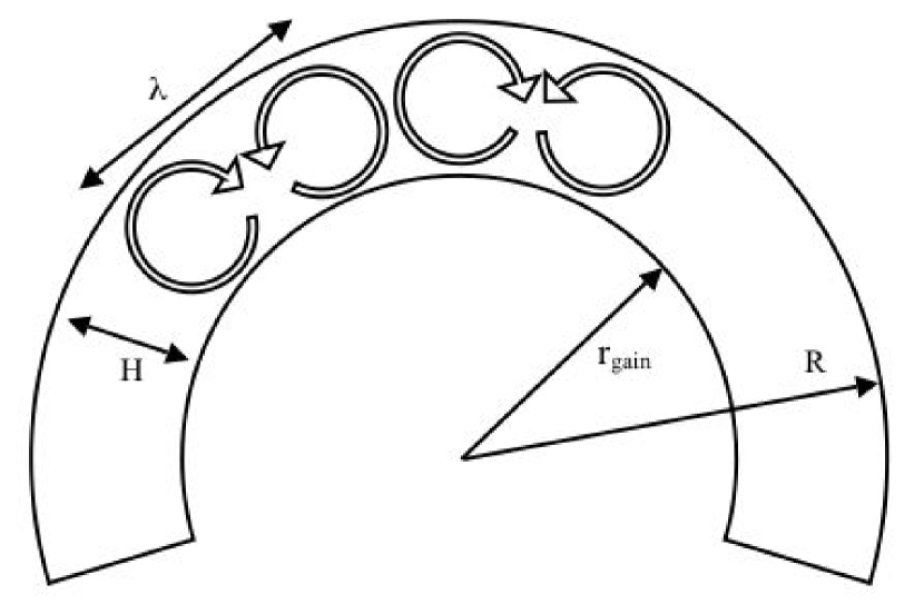
Figure 1: Schematic view of convection in a spherical shell of size $H$. The first unstable modes when viscosity is decreased have a wavelength $\lambda\sim(2$–$3)H$, depending on the boundary conditions (Chandrasekhar 1961)

In the absence of viscosity and of stabilizing composition gradients, a stratified atmosphere with a negative entropy gradient is unstable at all wavelengths. Perturbations with a horizontal wavelength shorter than the scale height $H$ of the entropy gradient are the most unstable. In a perfect gas with an adiabatic index $\gamma$, a measure of the entropy is defined by the dimensionless quantity $S$, as a function of pressure $P$ and density $\rho$:

$$S \equiv {1\over\gamma-1}\log\left[{P\over P_{\rm sh}}\left({\rho_{\rm sh}\over\rho}\right)^{\gamma}\right].$$ (1)

In this formula, pressure and density are normalized by their value immediately after the shock. In what follows, the subscript “sh” always refers to postshock quantities. The maximum growth rate ${\omega}_{\rm buoy}$ is given by the Brunt-Väisäla frequency, expressed by the gravitational acceleration $G$ and $H$:

$${\omega}_{\rm buoy} \equiv G^{1\over 2}\left|{\nabla P\over\gamma P}-{\nabla\rho\over\rho}\right|^{1\over 2}=\left({\gamma-1\over\gamma}G\nabla S\right)^{1\over 2},$$ (2)

$$\sim \left({G\over H}\right)^{1\over 2}.$$

Perturbations with a longer horizontal wavelength than $H$ are also unstable, with a slower growth rate however. Perturbations with a horizontal wavelength much shorter than $H$ are easily stabilized by a small amount of viscosity. This is illustrated by the calculations of Chandrasekhar (1961) of the onset of convection, either between two parallel plates or in a spherical shell. These calculations measured the amount of viscosity which is required to stabilize a perturbation with a given wavelength. The wavelength of the first unstable mode is about $[2-3]$ times the vertical size of the unstable region depending on the nature of the boundaries (free, rigid or mixed). Note that a factor 2 would be rather intuitive, since it corresponds to a pair of two counter-rotating circular eddies (see Fig. 1). In a spherical shell, a naive estimate of the azimuthal number $l$ of the first unstable perturbations, based on the number of pairs of circular eddies which would fit in the unstable shell $r_{\rm gain}<r<R$, leads to:

$$l\sim{\pi\over 2}{R+r_{\rm gain}\over H}\ .$$ (3)

This simplistic approach is compatible with the exact calculations performed by Chandrasekhar (1961), within the same factor $1-2$ as in the case of Benard convection (Rayleigh 1916). This factor depends on the boundary conditions, on the gravity profile, and can be interpreted as an aspect ratio of the eddies, which are not circular. A direct application to the size of a stalled shock with $R\sim 150$ km and $r_{\rm gain}\sim 100$ km, as in Herant, Benz & Colgate (1992), would lead to $l\sim 7$. As noted by Herant, Benz & Colgate (1992), the increase of $H$ naturally leads to the decrease of the optimal $l$. Is the residual instability of the $l=1$ mode fast enough to have a significant influence during the first second after core bounce? The classical description by Chandrasekhar is not directly applicable here, not only because viscosity is negligible, but also because it does not take into account the presence of a shock wave, and the associated flow of gas across it. Let us compare the timescale of buoyancy $\omega_{\rm buoy}^{-1}$ with the advection timescale $H/v_{\rm sh}$ through the gain region. The local gravity at the shock radius $r_{\rm sh}$ is $G\equiv{\cal G}M/r_{\rm sh}^{2}$, where ${\cal G}$ is the gravitational constant and $M$ is the enclosed gravitating mass. In what follows, the subscript “1” refers to preshock quantities. Assuming that the gas is in free fall ahead of the shock ($v_{1}^{2}\sim 2{\cal G}M/r_{\rm sh}$), one estimates:

$${H\omega_{\rm buoy}\over v_{\rm sh}} \sim \left({{\cal G}M\over r_{\rm sh}v_{\rm sh}^{2}}\right)^{1\over 2}\left({H\over r_{\rm sh}}\right)^{1\over 2},$$ (4)

$$\sim 3.1\left({v_{1}\over 7v_{\rm sh}}\right)\left({H\over 0.4r_{\rm sh}}\right)^{1\over 2}.$$ (5)

A typical radius of the stalled shock is $r_{\rm sh}\sim 150$ km, and $0.3\leq H/r_{\rm sh}\leq 0.5$. The velocity jump across the shock would be $v_{1}/v_{\rm sh}=7$ for an adiabatic gas with $\gamma=4/3$. This ratio may increase up to $v_{1}/v_{\rm sh}\sim 10$ due to dissociation of iron into nucleons. Even then, the rough estimate of Eq. (5) indicates that the convective growth time is comparable to the advection time through the gain region.

3 Description of a planar toy model

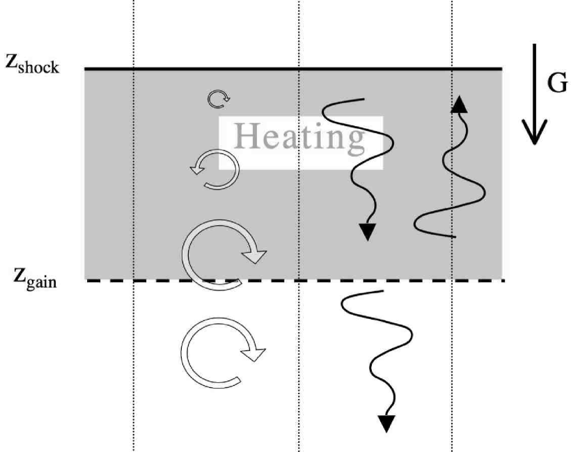
Figure 2: Schematic view of the toy model enabling the convective instability immediately below a shock. Heating dominates cooling in the gain region, so that the entropy gradient is oriented downward. Gravity $G$ is uniform. The flow below the gain radius is assumed to be uniform in the stationary regime, in order to preclude any acoustic feedback from below once perturbed. Entropy/vorticity perturbations (circular arrows) are advected downward with the flow. Acoustic perturbations (wavy arrows) propagate downward below the gain radius.

This Section establishes the equations describing a toy model in Cartesian geometry, illustrated by Fig. 2, in which only the minimum ingredients leading to the convective instability have been included. This toy model mimics in a most simplified form the accretion flow in the gain region immediately below the stalled accretion shock, a few tens of milliseconds after core bounce. The eigenmodes are solved numerically in Sect. 4.

3.1 Stationary flow

3.1.1 General description

The stationary flow is parallel along the $z$ direction, in a uniform gravity $G$. Self-gravity is neglected. A shock is stationary at the height $z_{\rm sh}$. The flow is described by a perfect gas with an adiabatic index $\gamma=4/3$, corresponding to a gas of relativistic electrons or photons and electron-positron pairs. We shall further assume that $P\propto\rho T$ (with $T$ being the temperature), which is a suitable description of the thermodynamic conditions in the gain layer independent of whether relativistic particles or baryons dominate the pressure (for details, see Janka 2001, Bethe 1993). The essential ingredients of the convective instability are the entropy changes and the local acceleration. In the gain region, the local acceleration is mainly due to the gravity $G$. The entropy gradient ${\nabla S}$ is produced by the heating through neutrino absorption, which exceeds the cooling by neutrino emission in the gain region. The heating/cooling function ${\cal L}$ is adapted from Bethe & Wilson (1985), neglecting the effect of geometric dilution of the neutrino flux:

$${\cal L} \equiv {{\bar{\cal L}}\rho\over 1-\beta}\left[1-\beta\left({T\over T_{\rm sh}}\right)^{6}\right],$$ (6)

$${\bar{\cal L}} \sim 2.2\left({r_{\rm sh}\over 150{\rm km}}\right)^{-2}\times 10^{20}{\rm ergs\;g^{-1}\;s^{-1}},$$ (7)

where $T_{\rm sh}$ is the postshock temperature. The parameter $\beta<1$ is defined as the ratio of the strengths of neutrino cooling and neutrino heating at the shock. The gain radius $z_{\rm gain}$ is defined as the point where ${\cal L}=0$. According to Eq. (6), the temperature at the gain radius is $T_{\rm gain}=T_{\rm sh}/\beta^{1\over 6}$. The temperature contrast $\Delta T_{\rm gain}/T_{\rm sh}$ within the gain region is thus directly related to the parameter $\beta$ of the heating/cooling function through

$${\Delta T_{\rm gain}\over T_{\rm sh}}\equiv{T_{\rm gain}-T_{\rm sh}\over T_{\rm sh}}={1\over\beta^{1\over 6}}-1.$$ (8)

Heating and cooling are neglected above and below the gain region.
The equation of continuity, the Euler equation and the entropy equation defining the stationary flow in the gain region lead to the following differential system:

$${\partial\over\partial z}(\rho v) = 0\ ,$$ (9)

$${\partial\over\partial z}\left({v^{2}\over 2}+{c^{2}\over\gamma-1}+Gz\right) = {{\cal L}\over\rho v}\ ,$$ (10)

$${\partial S\over\partial z} = {{\cal L}\over Pv}\ ,$$ (11)

where the last relation makes use of $P\propto\rho T$, and the pressure force in the Euler equation has been transformed using the definition (1) of $S$ and the relation $c^{2}\equiv\gamma P/\rho$:

$${\nabla P\over\rho}=\nabla\left({c^{2}\over\gamma-1}\right)-{c^{2}\over\gamma}\nabla S.$$ (12)

3.1.2 Photodissociation at the shock

Although dissociation at the shock is not expected to be an important ingredient for the convective instability, it is taken into account because of its effect on the postshock velocity, and thus on the advection time through the gain region. The effect of dissociation can be crudely incorporated by assuming that it takes place immediately behind the shock. It is parametrized in Appendix A by a decrease of the postshock Mach number ${\cal M}_{\rm sh}$ below the adiabatic value ${\cal M}_{\rm ad}$:

$${\cal M}_{\rm sh}\leq{\cal M}_{\rm ad}\equiv\left[{2+(\gamma-1){\cal M}_{1}^{2}\over 2\gamma{\cal M}_{1}^{2}-\gamma+1}\right]^{1\over 2}.$$ (13)

Note that Mach number are defined as positive ${\cal M}\equiv|v|/c>0$. In the phase of a stalled accretion shock the gravitating mass is $M\sim 1.2\;M_{\sun}$ and the preshock sound speed is $c_{1}\sim 8.5\times 10^{8}{\rm cm\;s^{-1}}$. The incident Mach number ${\cal M}_{1}$ is estimated assuming free-fall velocity of the gas incident at the shock:

$$|v_{1}| \sim \left({2{\cal G}M\over r_{\rm sh}}\right)^{1\over 2},$$ (14)

$$\sim 4.6\left({r_{\rm sh}\over 150{\rm km}}\right)^{-{1\over 2}}\times 10^{9}{\rm cm\;s^{-1}},$$

$${\cal M}_{1} \sim 5.4\left({r_{\rm sh}\over 150{\rm km}}\right)^{-{1\over 2}}.$$ (15)

The incident Mach number is taken equal to ${\cal M}_{1}=5$ in the rest of the paper, so that ${\cal M}_{\rm ad}\sim 0.39$ if $\gamma=4/3$. A prescription ${\cal M}_{\rm sh}/{\cal M}_{\rm ad}=0.77$ accounting for dissociation corresponds to more realistic values of ${\cal M}_{\rm sh}\sim 0.3$, a velocity jump $v_{1}/v_{\rm sh}\sim 8.8$ and a jump of sound speed $c_{\rm sh}/c_{1}\sim 1.85$. Considering the full range $1/(\gamma{\cal M}_{1})<{\cal M}_{\rm sh}\leq{\cal M}_{\rm ad}$ allows us to explore the stability of a larger family of flows, and thus better understand the onset of convection. The extreme case ${\cal M}_{\rm sh}{\cal M}_{1}=1/\gamma$ corresponds to $c_{\rm sh}=c_{1}$ and $v_{1}/v_{\rm sh}=\gamma{\cal M}_{1}^{2}$ is refered to as the “isenthalpic shock”.

3.1.3 Dimensionless parameters of the toy model

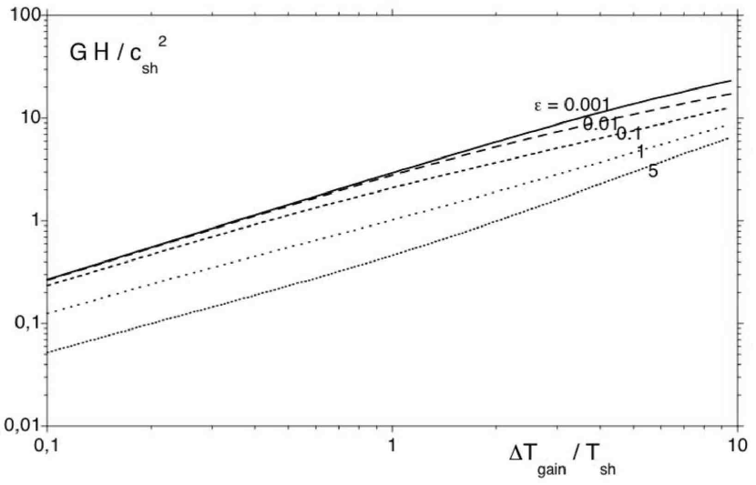
Figure 3: The power of heating, cooling and gravity are expressed through the dimensionless parameters $\epsilon$ and $\Delta T_{\rm gain}/T_{\rm sh}$. The resulting size $H\equiv z_{\rm sh}-z_{\rm gain}$ of the gain region is measured in units of $c_{\rm sh}^{2}/G$. The shock is adiabatic (${\cal M}_{1}=5$ in all plots).

The heating constant ${\bar{\cal L}}>0$ can be compared to the critical heating rate ${\bar{\cal L}}_{\rm crit}$ needed to cancel the velocity gradient immediately behind the shock, as deduced from Eqs. (9-11):

$${1\over v}{\partial v\over\partial z} = {1\over c^{2}-v^{2}}\left[G+(\gamma-1){{\cal L}\over\rho v}\right],$$ (16)

$${\bar{\cal L}}_{\rm crit} = -{Gv_{\rm sh}\over\gamma-1}.$$ (17)

The dimensionless parameter defined by $\epsilon\equiv{\bar{\cal L}}/{\bar{\cal L}}_{\rm crit}$ is thus a measure of the power of heating from the dynamical point of view. The flow is decelerated after the shock if $\epsilon<1$. Using a gravitating mass $M=1.2\;M_{\sun}$ in Eq. (17) and measuring the post-shock velocity in units of the free fall velocity $v_{1}$ (Eqs. 7 and 14), a typical value of $\epsilon$ is:

$$\epsilon \sim 0.16\;\left({v_{1}\over 7v_{\rm sh}}\right)\left({r_{\rm sh}\over 150{\rm km}}\right)^{1\over 2}.$$ (18)

In addition to $\gamma\sim 4/3$ and ${\cal M}_{1}\sim 5$, the independent parameters of this toy model are the dissociation parameter ${\cal M}_{\rm sh}/{\cal M}_{\rm ad}$, a measure of the heating rate at the shock through the parameter $\epsilon$, and the temperature contrast $\Delta T_{\rm gain}/T_{\rm sh}$ within the gain region. The parameters of this toy model allow for a wide variation of the size $H\equiv z_{\rm sh}-z_{\rm gain}$ of the gain region. This can be seen by integrating the differential system Eqs. (9-11) from the shock to the gain radius, with the function ${\cal L}$ described by Eq. (6). The corresponding results for a flow without dissociation are displayed in Fig. 3.

3.2 Linear perturbations

3.2.1 Differential system

The 1-D stationary flow is perturbed in the plane $x,z$, where $x$ is the horizontal direction. The complex frequency $\omega\equiv(\omega_{r},\omega_{i})$ of the perturbation is defined such that the real part $\omega_{r}$ is the oscillation frequency, and the imaginary part $\omega_{i}$ is the growth rate. The eigenmodes calculated in this study are non oscillatory ($\omega_{r}=0$). Rather than $\delta v_{x}$, $\delta v_{z}$, $\delta c$ and $\delta\rho$, the functions chosen for the perturbative approach are the entropy $\delta S$, and three functions $f$, $h$ and $\delta K$, defined by:

$$f \equiv v\delta v_{z}+{2\over\gamma-1}c\delta c\,,$$ (19)

$$h \equiv {\delta v_{z}\over v}+{\delta\rho\over\rho},$$ (20)

$$\delta K \equiv {ivk_{x}}\delta w_{y}+{k_{x}^{2}c^{2}\over\gamma}\delta S,$$ (21)

where $k_{x}$ is the horizontal wavenumber and $\delta w_{y}$ is the perturbation of vorticity. This choice is motivated by the fact that in the adiabatic limit, the perturbations $\delta S$ and $\delta K$ are conserved when advected (Foglizzo 2001, hereafter F01) and the coefficients of the differential system expressed with $f,h$ contain no radial derivative of the stationary flow quantities $v,c,{\cal M}$. If $\omega\neq 0$, the linearized equations are expressed by the following differential system of fourth order:

$${\partial f\over\partial z}={i\omega v\over 1-{{\cal M}^{2}}}\left\{h-{f\over c^{2}}+\left[\gamma-1+{1\over{{\cal M}^{2}}}\right]{\delta S\over\gamma}\right\}$$

$$+\delta\left({{\cal L}\over\rho v}\right),$$ (22)

$${\partial{h}\over\partial z}={i\omega\over v(1-{{\cal M}^{2}})}\left\{\frac{\mu^{2}}{c^{2}}f-{{\cal M}^{2}}{h}-\delta S\right\}$$

$$+{i\delta K\over\omega v},$$ (23)

$${\partial\delta S\over\partial z}={i\omega\over v}\delta S+\delta\left({{\cal L}\over pv}\right),$$ (24)

$${\partial\delta K\over\partial z}={i\omega\over v}\delta K+k_{x}^{2}\delta\left({{\cal L}\over\rho v}\right),$$ (25)

where $\mu$ is defined by:

$$\mu^{2}\equiv 1-{k_{x}^{2}c^{2}\over\omega^{2}}(1-{{\cal M}^{2}}).$$ (26)

$\mu$ is a natural parameter in the algebraic formulation of the problem. When the frequency $\omega$ is real, $\mu$ is directly related to the angle $\psi$ between the direction of propagation of the wave and the direction of the flow. Correcting a typing error in Eq. (E11) of F02:

$$\tan^{2}\psi = {1-\mu^{2}\over\mu^{2}(1-{\cal M}^{2})}.$$ (27)

In the differential system (22-25), the perturbations $\delta({\cal L}/\rho v)$ and $\delta({\cal L}/Pv)$ can be expressed in terms of $f,h,\delta S$ using Eqs. (19-20) and a perturbation of Eq. (6) (see Appendix B).

3.2.2 Boundary condition at the shock

The boundary conditions at the shock surface are obtained in Appendix C.1 using conservation laws in the frame of the perturbed shock:

$$f_{\rm sh} = \Delta v(v_{\rm sh}-v_{1})-\Delta\zeta\frac{c_{\rm sh}^{2}}{\gamma}\nabla{S}_{\rm sh},$$ (28)

$$h_{\rm sh} = {\Delta v\over v_{\rm sh}}\left(1-{v_{\rm sh}\over v_{1}}\right),$$ (29)

$${\delta S_{\rm sh}\over\gamma} = -\Delta\zeta\left[{\nabla S_{\rm sh}\over\gamma}+\left(1-{v_{\rm sh}\over v_{1}}\right){G\over c_{\rm sh}^{2}}\right]$$ (30)

$$-{v_{1}\Delta v\over c_{\rm sh}^{2}}\left(1-{v_{\rm sh}\over v_{1}}\right)^{2},$$

$$\delta K_{\rm sh} = -k_{x}^{2}\Delta\zeta\frac{c_{\rm sh}^{2}}{\gamma}\nabla{S}_{\rm sh}\ ,$$ (31)

where the velocity of the shock is related to its displacement through $\Delta v\equiv-i\omega\Delta\zeta$. In these equations, the cooling/heating above the shock is neglected (${\cal L}_{1}\ll{\cal L}_{\rm sh}$). These boundary conditions agree with FGR05 when heating is suppressed.

3.2.3 Leaking condition at the lower boundary

The effect of negative entropy gradients within the gain region are separated from any coupling process below the gain radius by choosing a leaking boundary condition at the gain radius:

- entropy and vorticity perturbations reaching the gain radius are simply advected downward,

- acoustic perturbations are free to propagate downward, with no reflexion.
This boundary condition is equivalent to replacing the accretion flow below the gain radius by a uniform flow. The uniformity of the unperturbed flow warrants the absence of coupling processes, once perturbed. Each perturbation is decomposed in Appendix C.2 as the sum of entropy, vorticity, and pressure perturbations:

$$f = f_{S}+f_{K}+f_{+}+f_{-}\ ,$$ (32)

$$h = h_{S}+h_{K}+h_{+}+h_{-}\ .$$ (33)

The absence of coupling below the gain radius corresponds to the absence of an acoustic flux from below ($f_{-}=0$, $h_{-}=0$). According to the calculation of Appendix C.2, this requirement is equivalent to the following condition:

$${\mu\over{\cal M}}{f\over c^{2}}-h-\left(\gamma+{\mu\over{\cal M}}{1-{\cal M}^{2}\over 1+\mu{\cal M}}\right){\delta S\over\gamma}$$

$$+{1-\mu^{2}\over 1+\mu{\cal M}}{\delta K\over k_{x}^{2}c^{2}}=0.$$ (34)

4 Convective mode in the gain region

4.1 Definition of the ratio ${\chi}$ comparing the advective and buoyancy timescales

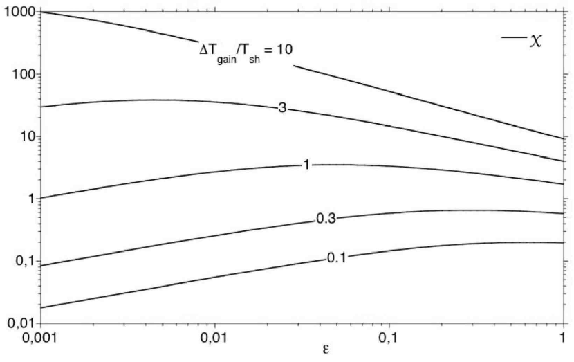
Figure 4: Ratio ${\chi}$ of the advective and convective timescales in our toy model with an adiabatic shock, as function of the heating parameter $\epsilon$, for different values of $\Delta T_{\rm gain}/T_{\rm sh}$ indicated on each curve.

The maximum growth rate $\omega_{\rm buoy}$ of the convective instability (Eq. 2) can be expressed with the local variables $\epsilon,T,v,c$ as a function of height $z$:

$${\omega}_{\rm buoy}(z) = \epsilon^{1\over 2}\left|{v_{\rm sh}\over v}\right|^{1\over 2}\left[{1-(T/T_{\rm gain})^{6}\over 1-(T_{\rm sh}/T_{\rm gain})^{6}}\right]^{1\over 2}{G\over c},$$ (35)

$${\omega}_{\rm max} \equiv {\rm Max}_{z_{\rm gain}<z<z_{\rm sh}}{\omega}_{\rm buoy}(z).$$ (36)

Note that $\epsilon^{1\over 2}$ directly measures the local growth rate of the convective instability at the shock, in units of $G/c_{\rm sh}$:

$${\omega}_{\rm buoy}^{\rm sh} = \epsilon^{1\over 2}{G\over c_{\rm sh}}.$$ (37)

When considered as a local instability, the transient amplification of short wavelength perturbations, during their advection through the gain region, can be estimated by the quantity $\exp{\chi}$, with

$${\chi} \equiv \int_{{\rm gain}}^{{\rm shock}}{\omega}_{\rm buoy}(z){{\rm d}z\over v}.$$ (38)

$\chi$ can be interpreted as the ratio of the advective timescale to some averaged timescale of convective growth. The correspondence between $\epsilon$, $\Delta T_{\rm gain}/T_{\rm sh}$ and $\chi$ is shown in Fig. 4.

4.2 Numerical solution of the eigenmode problem

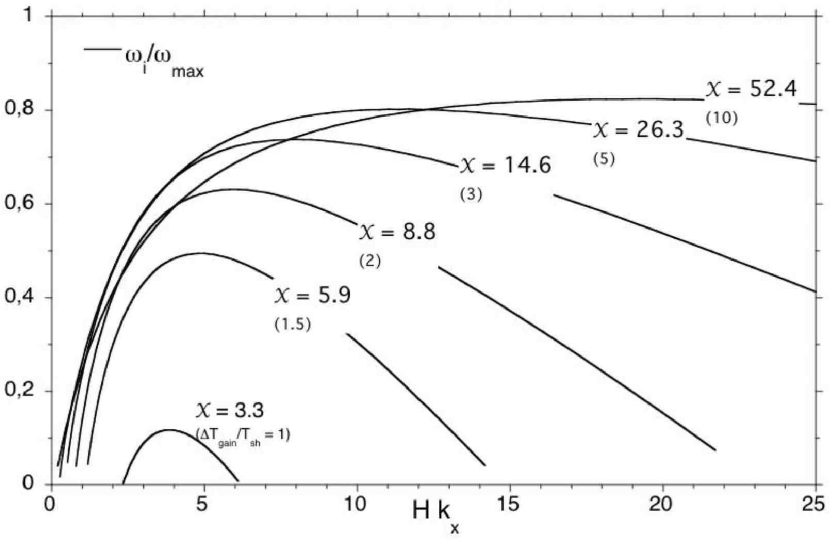
Figure 5: Growth rate $\omega_{i}$ of the convective instability as a function of the horizontal wavenumber. Growth rates are normalized to $\omega_{\rm max}$. Heating is such that $\epsilon=0.1$. The shock is adiabatic. The ratio ${\chi}$ of the advective and convective timescales is indicated on each curve, with the corresponding temperature contrast $\Delta T_{\rm gain}/T_{\rm sh}$ given in parentheses. Advection stabilizes both the long and short wavelengths. The convective instability disappears for ${\chi}<3$.

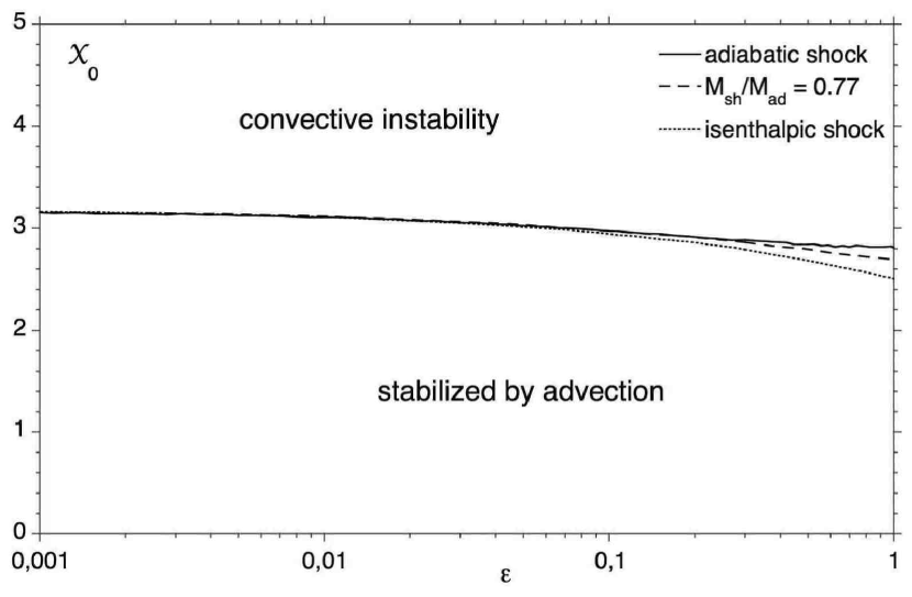
Figure 6: Threshold ${\chi}_{0}$ of the ratio of the convective and advective timescales, determining the existence of the convective mode, as a function of the power $\epsilon$ of heating. This threshold is essentially insensitive to dissociation at the shock.

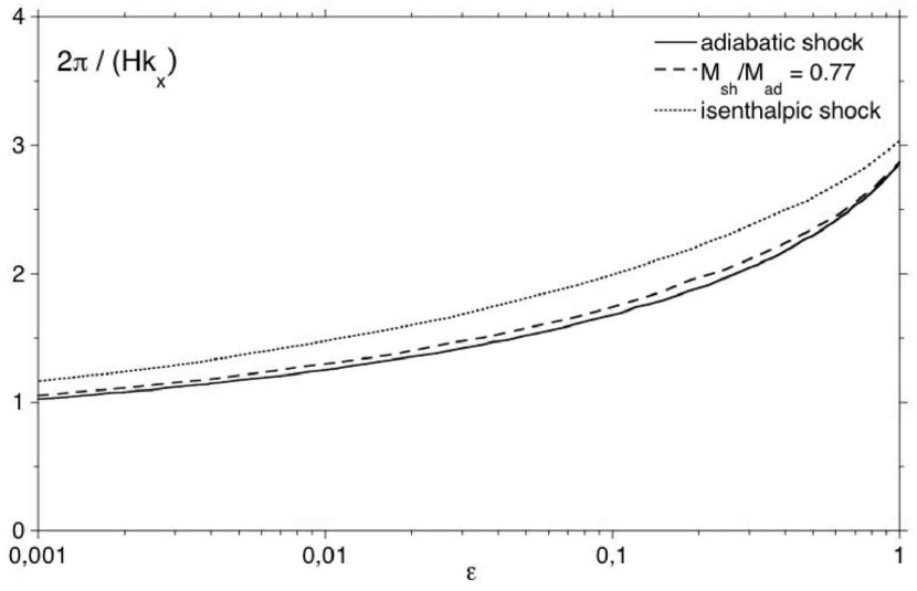
Figure 7: Wavelength of the neutral mode corresponding to the threshold value $\chi_{0}$, in units of the size of the gain region.

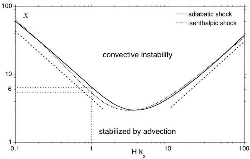
Figure 8: Range of horizontal wavenumbers allowing the convective instability, for $\epsilon=0.1$, when the ratio ${\chi}$ is varied as in Fig. 5. The slopes $\pm 1$ are indicated as dotted lines for comparison. A tentative generalization of these results to a spherical flow, in the spirit of Eq. (47), suggests that the convective instability of the $l=1$ mode in case of $H/r_{\rm sh}=0.5$ would require $\chi>6$ (Sect. 5.1). This is indicated by the vertical and horizontal dotted lines.

The numerical solution of the boundary value problem reveals that a global unstable mode grows exponentially with time if the advection timescale is long enough compared to the convective timescale. The existence of a global convective mode appears to depend directly on whether the ratio ${\chi}$, defined by Eq. (38), is above or below a certain threshold $\chi_{0}$.
As an illustration, Fig. 5 shows the effect of advection on the convective instability for $\epsilon=0.1$, where $1\leq\Delta T_{\rm gain}/T_{\rm sh}\leq 10$ is varied so that $3<{\chi}<53$. The convective growth is measured in units of $\omega_{\rm max}$, and the wavenumber in units of $H$. The classical convective instability is recovered in the limit ${\chi}\gg 1$. The effects of advection can be summarized as follows:

(i) The growth rate is decreased compared to the maximum value of the local convective growth rate $\omega_{\rm max}$ (Eq. (36)),

(ii) short wavelength perturbations are stable,

(iii) long wavelength perturbations are also stable.
In Fig. 5, the convective instability disappears completely for ${\chi}\leq 3$. The flow is then stable although the entropy gradient is negative. Even when the heating coefficient $\epsilon$ is varied over three orders of magnitude, the threshold of marginal stability always corresponds to ${\chi}_{0}\sim 3$, as shown in Fig. 6 for an adiabatic shock (full line). This threshold is approximately insensitive to the loss of energy at the shock through dissociation (dashed and dotted lines).
The stability threshold in Fig. 6 and in subsequent figures is obtained by solving the boundary value problem corresponding to the neutral mode (i.e. $\omega=0$), as described in Appendix D. According to Fig. 7, the wavelength of the neutral mode for $\chi=\chi_{0}$ is comparable to $[1-3]$ times the size $H$ of the gain region, with very little influence of dissociation at the shock. A similar range was obtained for the first unstable mode in classical convection stabilized by viscosity (Sect. 2).
The range of unstable wavenumbers decreases with ${\chi}$ in a very simple way illustrated by Fig. 8 for $\epsilon=0.1$. When measured in units of $1/H$, the minimal and maximal wavenumbers are proportional to ${\chi}^{-1}$ and ${\chi}$ respectively.

4.3 Towards a physical understanding

The existence of a stability threshold measured by $\chi$ can be interpreted in terms of energy. Approximating the entropy gradient $\nabla S\sim\Delta S/H$, the parameter $\chi^{2}$ is a measure of the potential energy in the gain region divided by the kinetic energy (i.e. the inverse of the Froude number ”${\rm Fr}$”):

$$\chi \sim \left({G\Delta S\over H}\right)^{1\over 2}{H\over v}\sim\left({GH\over v^{2}}\right)^{1\over 2}(\Delta S)^{1\over 2}\propto{\rm Fr}^{-{1\over 2}}.$$ (39)

The convective instability is driven by the potential energy, which is liberated by the interchange of high entropy and low entropy gas. The global instability requires that the energy gained from the interchange is large enough to overcome the kinetic energy of the gas. This qualitative interpretation does not explain, however, the relatively high value ($\chi_{0}\sim 3$) of the threshold. Besides, the simple scaling laws measured numerically in Fig. 8 call for a simple physical mechanism, yet to be determined.

5 Extrapolation to stalled accretion shocks in spherical geometry

This Section aims at discussing the validity of the results of Sect. 4 in a spherically symmetric flow, where convergence effects may play an important role. The effect of convergence is first estimated by a direct extrapolation of the results of Sect. 4. The outcome of this extrapolation is then compared to the result of a numerical determination of the eigenmodes in a spherical toy model. This successful comparison suggests that the results obtained may keep some relevance in the more complicated context of the core-collapse problem.

5.1 Tentative extrapolation of the parallel toy model

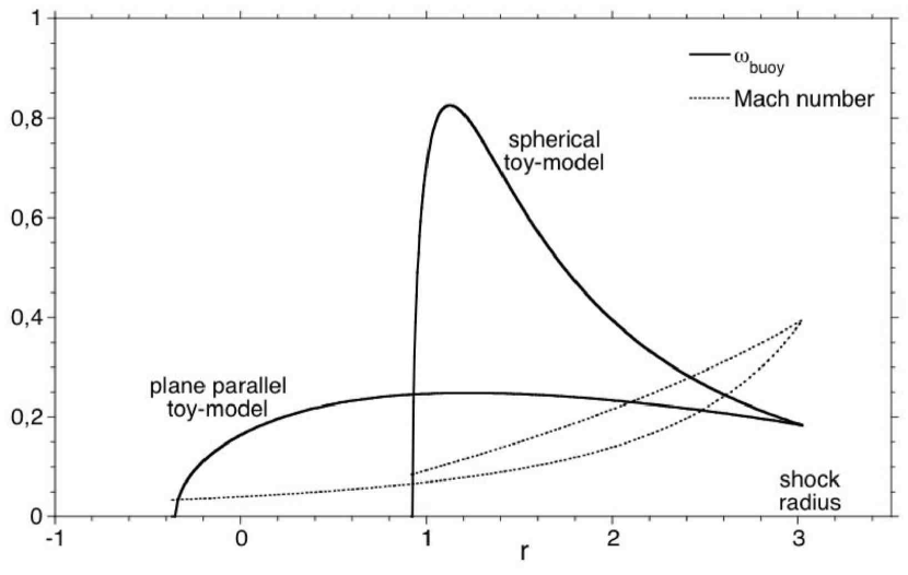
Figure 9: Two examples of the vertical shape of the local Brunt-Väisäla growth rate $\omega_{\rm buoy}(r)$ (full line) and Mach number (dotted line), in a plane parallel flow with constant gravity ($\chi=6.5$) and in a spherical flow ($\chi=4.1$). Distances are normalized by $c_{\rm sh}^{2}/G$ and growth rates by $G/c_{\rm sh}$, where $G$ is the strength of gravity at the shock radius. Both flows have the same heat flux at the shock. Buoyancy is maximum close to the gain radius in the spherical flow. In both cases, the buoyancy drops abruptly to zero at the gain radius.

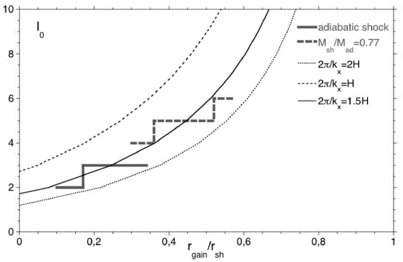
Figure 10: Degree $l$ of the first unstable mode in the spherical toy model for $\epsilon\leq 0.3$. The thin lines correspond to Eq. (48) extrapolated from the parallel toy model, with $2\pi/k_{x}=H$ (dashed line), $2\pi/k_{x}=1.5H$ (full line) and $2\pi/k_{x}=2H$ (dotted line).The thick lines correspond to the numerical solution of the eigenmodes in a spherical gain region with an adiabatic shock (full line) and with dissociation (dashed line).

The equations describing a spherical toy model and its perturbations are written in Appendix  E and solved numerically in the next subsection. The changes introduced in spherical symmetry appear on the stationary flow equations:

$${\cal L} \equiv {{\bar{\cal L}}\rho\over 1-\beta}\left[\left({r_{\rm sh}\over r}\right)^{2}-\beta\left({T\over T_{\rm sh}}\right)^{6}\right],$$ (40)

$${\partial\over\partial r}(\rho vr^{2}) = 0,$$ (41)

$${\partial\over\partial r}\left({v^{2}\over 2}+{c^{2}\over\gamma-1}-{{\cal G}M\over r}\right) = {c^{2}\over\gamma}{\partial S\over\partial r}.$$ (42)

Neutrino heating, gravity $G\equiv{{\cal G}M/r^{2}}$ and momentum $\rho v$ increase inward like $r^{-2}$. The radial shape of the Brunt-Väisäla frequency $\omega_{\rm buoy}(r)$ is modified accordingly:

$${\omega}_{\rm buoy} = {{\cal G}M\over cr_{\rm sh}^{2}}{r_{\rm sh}\over r}\left|{v_{\rm sh}\over v}\right|^{1\over 2}{(\alpha\epsilon)^{1\over 2}\over(1-\beta)^{1\over 2}}\left[\left({r_{\rm sh}\over r}\right)^{2}-\beta\left({T\over T_{\rm sh}}\right)^{6}\right]^{1\over 2}.$$ (43)

The critical heating leading to a postshock reacceleration is decreased by a factor $\alpha\sim 0.5$ due to the convergence of the flow so that $\epsilon$ is now defined as

$$\epsilon \equiv -{\gamma-1\over\alpha}{{{\bar{\cal L}}}r_{\rm sh}^{2}\over{\cal G}Mv_{\rm sh}}\ ,$$ (44)

$$\alpha \equiv 1-{2r_{\rm sh}c_{\rm sh}^{2}\over{\cal G}M}\ .$$ (45)

According to this new definition of $\epsilon$, its estimation for a spherical flow is:

$$\epsilon \sim 0.32\;\left({v_{1}\over 7v_{\rm sh}}\right)\left({r_{\rm sh}\over 150{\rm km}}\right)^{1\over 2}.$$ (46)

As illustrated on Fig. 9 for $r_{\rm gain}/r_{\rm sh}\sim 0.3$, the maximum value of $\omega_{\rm buoy}(r)$ may be reached close to the gain radius, and may exceed its value at the shock by a large factor. As seen in Appendix E, the structure of the perturbed equations (E2-E5) is the same as in the parallel toy model (Eqs. (22-25)), the main change consisting in replacing $k_{x}^{2}$ by $l(l+1)/r^{2}$. A tentative extrapolation of the results obtained in a parallel flow may use a mean radius $(r_{\rm sh}+r_{\rm gain})/2$ to translate the horizontal wavenumber $k_{x}$ into the degree $l$. This gives:

$$l^{1\over 2}(l+1)^{1\over 2}\sim{k_{x}\over 2}(r_{\rm sh}+r_{\rm gain})=k_{x}H\left({r_{\rm sh}\over H}-{1\over 2}\right).$$ (47)

Since the most unstable horizontal wavelength is comparable to $[1-2]$ times the vertical size of the gain region in the parallel flow (Fig. 7), the degree $l$ of the most unstable mode should be comparable to

$$l^{1\over 2}(l+1)^{1\over 2}\sim[1-2]\pi\left({r_{\rm sh}\over H}-{1\over 2}\right).$$ (48)

Applying in this formula $H/r_{\rm sh}\sim 0.5$ leads to $l\sim 6$ (thin full line in Fig. 10). This correspondence is certainly very crude for low degree modes. Nevertheless, it compares favorably to the results obtained numerically in spherical geometry in the next subsection (thick lines in Fig. 10). Making a similar extrapolation for the $l=1$ mode in a flow with $H/r_{\rm sh}\sim 0.5$, in which case Eq. (47) gives $k_{x}H\sim 1$, Fig. 8 suggests that this mode should be stabilized by advection unless ${\chi}>6$.

5.2 Numerical solution for the eigenmodes in a spherical toy model

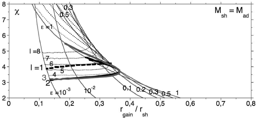
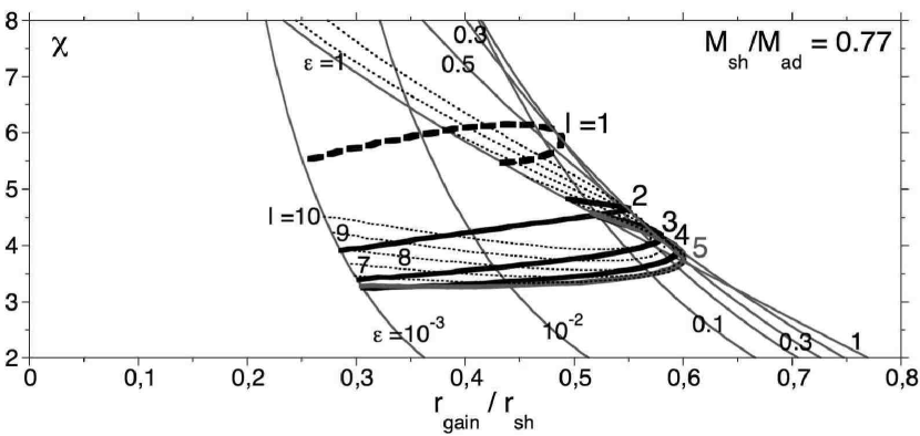
Figure 11: Instability threshold determined from solving numerically the boundary value problem associated to a toy model in spherical geometry. The thin full lines show the range of ($r_{\rm gain},\chi$) of the flows with a given value of the heating parameter $\epsilon$, indicated on each line, when the cooling parameter $\beta$ is varied. Nuclear dissociation is neglected in the upper plot, whereas $M_{\rm sh}/M_{\rm ad}=0.77$ in the lower plot. The curves labelled by $l$ (thick lines and thin dotted lines) show the stability threshold of a specific low degree perturbation, when the heating parameter $\epsilon$ is varied from $\epsilon=10^{-3}$ to $\epsilon=1$. The mode $l=1$ is associated with the thick dashed line. The most unstable modes correspond to $l\sim 2-3$ perturbations in flows without dissociation (upper plot), and $l=4-5-6$ with dissociation (bottom plot). In both cases, the global stability threshold corresponds to $\chi_{0}\sim 3$.

5.2.1 Range of $r_{\rm gain}/r_{\rm sh}$ and $\chi$ in our stationary, spherical toy model

The spherical geometry strongly limits the range of parameters ($r_{\rm gain}/r_{\rm sh},\chi$) that can be reached within reasonable values of neutrino heating ($\epsilon\leq 1$). Due to the geomatric dilution of neutrino heating in Eq. (40), the temperature contrast with the gain region $\Delta T_{\rm gain}/T_{\rm sh}$ is no longer an explicit parameter $\beta$ of the cooling function, because Eq. (8) is now replaced by

$${\Delta T_{\rm gain}\over T_{\rm sh}}={1\over\beta^{1\over 6}}\left({r_{\rm sh}\over r_{\rm gain}}\right)^{1\over 3}-1.$$ (49)

It is thus more convenient to use the parameters ($\epsilon,\beta$) to define a toy model in spherical symmetry. The thin full lines of Fig. 11 show how the parameter space ($\epsilon,\beta$) can be mapped into the plane ($r_{\rm gain}/r_{\rm sh},\chi$). This mapping is folded near $\epsilon\sim 0.3$. Note that this folding is also present in the plane parallel toy model, as can be deduced from Figs. 3 and 4. In spherical geometry, high values of $\chi$ can only be obtained in flows with a small gain radius. Even with the decelaration due to dissociation (right plot of Fig. 11), the flows where $r_{\rm gain}/r_{\rm sh}>0.6$ have a very moderate parameter $\chi<4$.

5.2.2 Numerical solution of the boundary value problem

The stability analysis of this family of flows is summarized by the thick full lines and thin dotted lines of Fig. 11, obtained as follows: for each heating parameter $\epsilon$ in the range $10^{-3}\leq\epsilon\leq 1$, a parameter $\beta(\epsilon,l)$ is determined such that the corresponding flow is marginally stable with respect to perturbations of degree $l$. The value of the gain radius and $\chi$ of this flow is then plotted.

- In both plots, the threshold for convective instability corresponds to $\chi_{0}\sim 3$, as in plane parallel flows.

- The degree $l$ of the first unstable mode, plotted in Fig. (10) is surprisingly close to the rough estimate extrapolated from the parallel toy model (Eq. (48)) for $\epsilon\leq 0.3$.

- The destabilization of the mode $l=1$ is slightly easier than anticipated by the plane parallel toy model. The threshold $\chi_{0}^{1}$ for this mode is in the range $[4,6]$, whereas Fig. 8 would suggest $\chi_{0}^{1}\sim 6\pm 1$. Moreover, dissociation surprisingly increases the $l=1$ threshold in a spherical flow, while it would be slightly decreased according to Fig. 8.

6 Comparison to supernova simulations

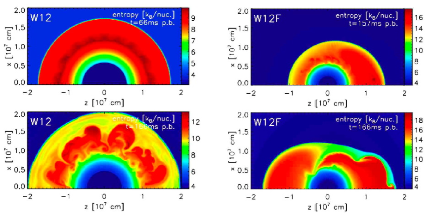
Figure 12: Results of two hydrodynamic simulations (in 2D) of the post-bounce accretion phase of a stalled supernova shock. The plots on the left show snapshots (at $t=66\,$ms and 166 ms after bounce) from a model with slow neutron star contraction and $\chi=5$. In this case convection develops in the neutrino-heating layer with a dominant $l=4\,$–$\,5$ mode. The right plots display the situation for a more rapidly contracting neutron star, in which case $\chi=2.5$. As predicted by the analytic toy model of Sect. 5, convection is unable to grow for these conditions. The visible instability of an $l=1$ mode is oscillatory and distinctively different from the development of convection in the other case. This asymmetry is interpreted as the consequence of a global nonradial instability of the accretion shock, which is of advective-acoustic nature. Entropy inhomogeneities created by the oblique shock then seed the growth of Rayleigh-Taylor mushrooms as a secondary phenomenon.

The perturbative analysis presented here was accompanied by two-dimensional hydrodynamic simulations of the accretion phase of stalled supernova shocks after core bounce. While the details of these numerical experiments will be reported elsewhere (Scheck et al., in preparation), we will discuss some of the results here in order to link the conclusions from the simplified toy model to the flow dynamics found in more complete hydrodynamic simulations of the conditions in supernova cores.

The simulations were performed with the computational setup described in Scheck et al. (2006). We used the Riemann-solver based Prometheus hydrodynamics code, which was supplemented by an approximative (grey) description of the neutrino transport. This allowed us to follow the effects of neutrino cooling and heating and their backreaction on the neutrino fluxes. The simulations made use of a physical equation of state of the stellar plasma including leptons, photons, and baryons. The baryonic composition is assumed to be given by neutrons, protons, alpha particles, and a representative heavy nucleus in nuclear statistical equilibrium, thus ensuring the inclusion of nuclear photodisintegration effects. The two-dimensional models were computed with a polar grid and started from spherically symmetric post-bounce conditions of the collapsing core of a 15$\,M_{\odot}$ star, perturbing the initial data for seeding convection. In order to compare the numerical simulations with the analytic analysis, these perturbations must be sufficiently small to trigger the onset of instability in the linear regime. The inner, high-density core of the neutron star was replaced by a gravitating point mass and a Lagrangian (and thus closed) boundary at a chosen, shrinking radius to mimic the contracting nascent neutron star. The neutrino fluxes and mean flux energies at this boundary (which is typically located at an optical depth much larger than 10 for all neutrino flavors) were prescribed as functions of time.

The behavior of a model depends on the motion of the inner grid boundary and the size of the boundary fluxes. When the latter are sufficiently high, the model develops an explosion; when the luminosities are below some critical value, no explosion can occur. The influence of the boundary motion is more subtle. On the one hand, it directly affects the development of nonradial hydrodynamic instabilities in the postshock layer, a fact which will be used below for setting up special conditions in the supernova core. On the other hand, it determines the amplification of the neutrino luminosities in the settling surface layer of the contracting neutron star. The faster the neutron star contracts, the more it heats up by the conversion of gravitational energy to internal energy. As a consequence, the accretion luminosity becomes higher. This produces stronger neutrino heating behind the shock and thereby has a bearing on the supernova dynamics.

The direct influence of the boundary contraction results from the fact that the accretion shock follows the boundary behavior when nonradial hydrodynamic instabilities are absent and the neutrino luminosities are not close to the critical value for causing an explosion. A more compact neutron star thus leads to a smaller shock radius and correspondingly higher infall velocities ahead of and behind the shock. Since the gain layer is also more narrow, the advection timescale of the accreted gas and therefore the parameter $\chi$ in the gain layer is significantly reduced. This dependence allowed us to tune the possibility for the development of convective instability through the chosen contraction of the inner boundary.

Figure 12 shows snapshots from two such numerical experiments. The plots on the left result from a simulation (Model W12 from Scheck et al. 2006) with a slowly contracting neutron star and therefore a large value of $\chi_{\mathrm{W12}}=5$, which enables the gain layer to become convectively unstable ($r_{\mathrm{gain}}/r_{\mathrm{sh}}\approx 0.6$ in this model at $t\gtrsim 65\,$ms after bounce). As predicted by the perturbative analysis in Sect. 5 (see the case with nuclear dissociation in Fig. 11), the most unstable and fastest growing mode is found to have $l=4\,$–$\,5$ and a corresponding wavelength of about $2H$. Note that for clean diagnostics, the power distribution of the initial seed must not disfavor this wavelength compared to others (as, e.g. random zone-to-zone seed perturbations do).

The right plots display the situation for a more rapidly contracting neutron star (Model W12F of Scheck et al. 2006), in which case we determined $\chi\approx 2.5$. In agreement with the analytic toy model, convection does not develop in the first place here. The bipolar sloshing mode and $l=1$ deformation that grows instead is distinctively different from the dynamics of the other case and not of convective nature, but is interpreted as a nonradial accretion shock instability that originates from an advective-acoustic cycle in the volume between shock and neutron star surface. This will be further analyzed and discussed in a forthcoming paper (Scheck et al., in preparation). Subsequently, convective activity is seeded by the increasingly larger entropy perturbations that are created in the accretion flow when it passes the deformed shock obliquely. This is visible in the right panels of Fig. 12 in mushroom-like Rayleigh-Taylor fingers showing up. Numerical experiments like these with a more “realistic” description of the supernova conditions therefore confirm the conclusions drawn from the toy model (whose free parameters and crucial features were, of course, designed to accommodate the physical conditions during the stalled shock accretion phase).

We point out, however, that simulations of the full supernova problem are complex and can involve factors which can make it harder to unambiguously disentangle the action of different instabilities and their properties than for the described specific setups. Of particular relevance in this respect are the properties of the perturbations that trigger the growth of convection. If the seed power of the most unstable convective mode is much lower than for other wavelengths, for example, the growth of these other modes may initially be favored. In case of large perturbation amplitudes on the other hand, the conditions for the linear regime of the analytic analysis may not be fulfilled and buoyant bubble floating may set in even if the linear analysis predicts convective stability of the accretion flow. A comparison of numerical simulations with the analytic discussion therefore requires special care.

7 Conclusions

A toy model has been developed and studied in depth in order to understand the effect of advection on the linear growth of the convective instability in the gain region immediately below a stationary shock. New results have been obtained through a numerical calculation of the eigenmodes and extrapolated to core-collapse flows.

(i) The numerical solution of the boundary value problem reveals that convection can be significantly stabilized by advection. The existence of a negative entropy gradient is not a sufficient condition for the convective instability in an advected flow. Not only the growth rate of the fastest growing mode is diminished, but also the range of unstable wavelengths is modified.

- The effect of advection on the convective instability is essentially governed by a single dimensionless parameter $\chi$, defined by Eq. (38), which compares the buoyant and the advection timescales.

- As illustrated in Fig. 5, a convective mode may develop in the gain region, with a linear growth rate significantly slower than the local convective growth rate if the value of $\chi$ is moderate ($3<\chi<5$). In the plane parallel flow of our toy model, the gain region is linearly stable if $\chi<3$.

- The minimum and maximum unstable wave numbers are directly related to $\chi$ according to $Hk_{\rm min}\propto 1/\chi$, $Hk_{\rm max}\propto\chi$ as shown in Fig. 8.

- The horizontal wavelength of the first unstable mode when $\chi\sim 3$ is comparable to twice the vertical size of the gain region.

(ii) These results can be used as a guide to better understand the convective motions behind a stalled accretion shock in core collapse supernovae, and in particular their contribution to an $l=1$ asymmetry. The parameter $\chi$ can be measured directly in numerical simulations. A rough estimate, in Eq. (5), suggests that $\chi$ may be close to the threshold of stabilization. The stabilization of long wavelength perturbations, illustrated by Fig. 5 and Fig. 8, can be a severe impediment to the development of a residual $l=1$ mode. The solution of the eigenvalue problem in a spherical toy model confirms the threshold $\chi_{0}\sim 3$ for the convective instability, and shows examples where the mode $l=1$ is stable unless $\chi>4-6$. A comparison with numerical simulations for supernova conditions supports the conclusions of our toy model.

To what extent should we expect the threshold $\chi_{0}\sim 3$ to be valid in the more complicated setup of core-collapse simulations ? Although we did not provide a quantitative explanation for this particular value, it is remarkable that the threshold seems to be affected very little ($2.6<\chi_{0}<3.2$) by significant changes in the flow parameters, including both the heating and cooling parameters and the photodissociation at the shock (Fig. 6). This threshold is also independent of the geometry; the same value applies for plane parallel and spherical conditions (Fig. 11).

We should stress again an important hypothesis of our toy model concerning the boundary condition at the gain radius: a leaking boundary condition isolates the gain region from any possible acoustic feedback from below the gain radius. The threshold $\chi_{0}\sim 3$ thus sets the limit of a convective instability fed by the gain region alone. Whether coupling processes taking place below the gain radius may or may not help convective motions to develop, cannot be answered by the present study. Preliminary results by Yamasaki & Yamada (2006), showing an instability for $\chi<3$, could be interpreted as partially fed by an acoustic feedback from below the gain radius.

More generally, our results do not preclude the possible destabilization of the $l=1$ mode due to coupling processes occurring below the gain radius (Blondin et al. 2003, Galletti & Foglizzo 2005, Scheck et al. 2004, 2006, Ohnishi, Kotake & Yamada 2006, Burrows et al. 2006). The study of such global cycles, and their possible interaction with convection, is the subject of forthcoming papers which consider a linear analysis (Foglizzo et al. 2006) as well as numerical simulations of the nonlinear growth of nonspherical modes in the supernova core (Scheck et al., in preparation).

Appendix A Photodissociation at the shock

The energy cost of dissociation is ${\cal E}\sim 8.8$MeV per nucleon for iron. This energy is assumed to be lost immediately after the shock. It affects the conservation of the Bernoulli constant across the shock as a sink term ${\cal E}$ on the post-shock side:

$${v_{1}^{2}\over 2}+{c_{1}^{2}\over\gamma-1}={v_{\rm sh}^{2}\over 2}+{c_{\rm sh}^{2}\over\gamma-1}+{\cal E}.$$ (A1)

The conservation of mass flux $\rho v$ and momentum flux $P+\rho v^{2}$ across the shock are unchanged by photodissociation. Writing $P=\rho c^{2}/\gamma$, these two equation are:

$$\rho_{1}v_{1} = \rho_{\rm sh}v_{\rm sh},$$ (A2)

$$\rho_{1}{c_{1}^{2}\over\gamma}+\rho_{1}v_{1}^{2} = \rho_{\rm sh}{c_{\rm sh}^{2}\over\gamma}+\rho_{\rm sh}v_{\rm sh}^{2}.$$ (A3)

The classical Rankine-Hugoniot jump conditions are replaced by the following formulation, obtained after some algebra with Eqs. (A1-A3):

$${{\cal E}\over{v_{1}^{2}\over 2}+{c_{1}^{2}\over\gamma-1}} = \left(1-{{\cal M}_{\rm sh}^{2}\over{\cal M}_{\rm ad}^{2}}\right)\left(1-{{\cal M}_{\rm sh}^{2}\over{\cal M}_{1}^{2}}\right),$$ (A4)

$${v_{\rm sh}\over v_{1}} = {{\cal M}_{\rm sh}^{2}\over{\cal M}_{1}^{2}}{1+\gamma{\cal M}_{1}^{2}\over 1+\gamma{\cal M}_{\rm sh}^{2}},$$ (A5)

$${c_{\rm sh}\over c_{1}} = {{\cal M}_{\rm sh}\over{\cal M}_{1}}{1+\gamma{\cal M}_{1}^{2}\over 1+\gamma{\cal M}_{\rm sh}^{2}}.$$ (A6)

Using Eq. (A4), we choose to parametrize the effect of dissociation by the value of the postshock Mach number ${\cal M}_{\rm sh}\leq{\cal M}_{\rm ad}$. According to Eqs. (A5) and (A6), $v_{1}/v_{\rm sh}=\gamma{\cal M}_{1}^{2}$ and $c_{\rm sh}=c_{1}$ if ${\cal M}_{\rm sh}{\cal M}_{1}=1/\gamma$. This rather extreme case is refered to as the “isenthalpic shock”.

Appendix B Expression of the perturbed heating/cooling function

Using the fact that $\delta T/T=\delta c^{2}/c^{2}$, the heating function described by Eq. (6) is perturbed as follows:

$$\delta\left({{\cal L}\over\rho v}\right) = -{\nabla S}{c^{2}\over\gamma}{\delta v_{z}\over v}-{6\beta{\nabla S}_{\rm sh}\over\gamma(1-\beta)}{v_{\rm sh}\over v}c_{\rm sh}^{2}\left({c\over c_{\rm sh}}\right)^{12}{\delta c^{2}\over c^{2}},$$ (B1)

$$\delta\left({{\cal L}\over pv}\right) = {\gamma\over c^{2}}\delta\left({{\cal L}\over\rho v}\right)-{\delta c^{2}\over c^{2}}{\nabla S},$$ (B2)

In these equations, the perturbations $\delta v_{z}$ and $\delta c$ can be replaced by functions of $f,h,\delta S$ using Eq. (1) and Eqs. (19-20):

$${\delta v_{z}\over v} = {1\over 1-{\cal M}^{2}}\left(h-{f\over c^{2}}+{\delta S}\right),$$ (B3)

$${\delta c^{2}\over c^{2}} = {\gamma-1\over 1-{\cal M}^{2}}\left({f\over c^{2}}-{\cal M}^{2}{h}-{\cal M}^{2}{\delta S}\right).$$ (B4)

Appendix C Boundary conditions

C.1 Shock boundary condition

The boundary condition at the shock are established in this Appendix, following the conservation of mass flux, momentum flux and energy flux in the frame of the shock:

$$\rho_{1}(v_{1}-\Delta v) = (\rho_{{\rm sh}}+\delta\rho_{\rm sh})(v_{{\rm sh}}+\delta v_{{\rm sh}}-\Delta v),$$ (C1)

$$\rho_{1}(v_{1}-\Delta v)^{2}+\rho_{1}{c_{1}^{2}\over\gamma} = (\rho_{{\rm sh}}+\delta\rho_{\rm sh})(v_{{\rm sh}}+\delta v_{{\rm sh}}-\Delta v)^{2}$$ (C2)

$$+(\rho_{{\rm sh}}+\delta\rho_{\rm sh}){(c_{{\rm sh}}+\delta c_{{\rm sh}})^{2}\over\gamma},$$

$${(v_{1}-\Delta v)^{2}\over 2}+{c_{1}^{2}\over\gamma-1} = {(v_{{\rm sh}}+\delta v_{{\rm sh}}-\Delta v)^{2}\over 2}+{(c_{{\rm sh}}+\delta c_{{\rm sh}})^{2}\over\gamma-1}$$ (C3)

$$+{\cal E},$$

where $\delta v_{\rm sh}$ stands for the vertical component of the perturbed velocity, and quantities are measured at the position ${r}_{\rm sh}+\Delta\zeta$. Keeping the first order terms, and using the defnition of $f,h$, these equations are rewritten at the position ${r}_{\rm sh}$ using a Taylor expansion:

$$\rho_{1}v_{1}h_{\rm sh}-(\rho_{{\rm sh}}-\rho_{1})\Delta v=,$$

$$\Delta\zeta\left[{\partial\over\partial z}\left(\rho v\right)_{1}-{\partial\over\partial z}\left(\rho v\right)_{\rm sh}\right],$$ (C4)

$$v_{{\rm sh}}^{2}\delta\rho_{\rm sh}+2\rho_{\rm sh}v_{\rm sh}\delta v_{\rm sh}+{2\over\gamma}\rho_{{\rm sh}}c_{{\rm sh}}\delta c_{{\rm sh}}+\delta\rho_{\rm sh}{c_{{\rm sh}}^{2}\over\gamma}=$$

$$\Delta\zeta\left[{\partial\over\partial z}\left(\rho v^{2}+\rho{c^{2}\over\gamma}\right)_{1}-{\partial\over\partial z}\left(\rho v^{2}+\rho{c^{2}\over\gamma}\right)_{\rm sh}\right],$$ (C5)

$$f_{\rm sh}-(v_{\rm sh}-v_{1})\Delta v=$$

$$\Delta\zeta\left[{\partial\over\partial z}\left({v^{2}\over 2}+{c^{2}\over\gamma-1}\right)_{1}-{\partial\over\partial z}\left({v^{2}\over 2}+{c^{2}\over\gamma-1}\right)_{\rm sh}\right],$$ (C6)

The local gradients in these three equations are computed from Eqs. (9), (10), (11) describing the stationary flow,

$${\partial\over\partial z}\left(\rho v\right) = 0,$$ (C7)

$${\partial\over\partial z}\left(\rho v^{2}+\rho{c^{2}\over\gamma}\right) = -G\rho,$$ (C8)

$${\partial\over\partial z}\left({v^{2}\over 2}+{c^{2}\over\gamma-1}\right) = {{\cal L}\over\rho v}-G.$$ (C9)

We obtain:

$$h_{\rm sh} = \left({1\over v_{{\rm sh}}}-{1\over v_{1}}\right)\Delta v,$$ (C10)

$${\delta S_{\rm sh}\over\gamma} = {\Delta\zeta\over c_{\rm sh}^{2}}\left[{{\cal L}_{1}\over\rho_{1}v_{1}}-{{\cal L}_{\rm sh}\over\rho_{\rm sh}v_{\rm sh}}-G\left(1-{v_{\rm sh}\over v_{1}}\right)\right]$$ (C11)

$$-{v_{1}\Delta v\over c_{\rm sh}^{2}}\left(1-{v_{\rm sh}\over v_{1}}\right)^{2},$$

$$f_{\rm sh} = (v_{{\rm sh}}-v_{1})\Delta v+\Delta\zeta\left({{\cal L}_{1}\over\rho_{1}v_{1}}-{{\cal L}_{\rm sh}\over\rho_{\rm sh}v_{\rm sh}}\right).$$ (C12)

The assumption that ${\cal L}_{1}\ll{\cal L}_{\rm sh}$ leads to Eqs. (28), (29) and (30).
$\delta K$ is rewritten using its definition (Eq. 21) and the transverse component of the linearized Euler equation:

$$\delta K=k_{x}^{2}f-\omega k_{x}\delta v_{x}.$$ (C13)

The transverse velocity immediately after the shock is deduced from the conservation of the tangential component of the velocity, in the spirit of Landau & Lifschitz (1989).

$$(\delta v_{x})_{\rm sh} = (v_{1}-v_{{\rm sh}})ik_{x}\Delta\zeta,.$$ (C14)

Finally, Eq. (31) is deduced from Eq. (C13), with Eqs. (C14) and (28).
The vorticity $\delta w_{y}$ produced by the perturbed shock, deduced from Eqs. (21), (30) and (31), is independent of heating:

$$(\delta w_{y})_{\rm sh}=-{ik_{x}\over v_{\rm sh}}\left(1-{v_{\rm sh}\over v_{1}}\right)\left[(v_{1}-v_{\rm sh})\Delta v+G\Delta\zeta\right].$$ (C15)

C.2 Lower boundary condition

Establishing the leaking boundary condition requires to identify the acoustic content of the perturbation $f$ as it reaches the lower boundary. For this purpose, we use the classical decomposition into acoustic and advected perturbations (i.e. Landau & Lifschitz 1989) in an adiabatic, uniform flow. The perturbation $f_{S}$ associated with an advected entropy perturbation $\delta S$ such that $\delta K=0$, and the perturbation $f_{K}$ associated to $\delta K$ with $\delta S=0$ are deduced from the differential system (22-25), in which ${\cal L}\equiv 0$ (adiabatic flow) and ${\rm d}/{\rm d}z\equiv i\omega/v$ (advected perturbations):

$$f_{S} = {1-{\cal M}^{2}\over 1-\mu^{2}{\cal M}^{2}}c^{2}{\delta S\over\gamma}\ ,$$ (C16)

$$f_{K} = {{\cal M}^{2}(1-\mu^{2})\over 1-\mu^{2}{\cal M}^{2}}{\delta K\over k_{x}^{2}}\ .$$ (C17)

Both are associated with the same wave number $k_{z}^{0}$ of advected perturbations:

$$k_{z}^{0}={\omega\over v}.$$ (C18)

Pressure perturbations $f_{\pm}$ correspond to the solution of the differential system (22) to (25) with ${\cal L}=0$, $\delta S=0$ and $\delta K=0$. The longitudinal wavenumber $k^{\pm}$ of acoustic perturbations is equal to

$$k^{\pm}\equiv{\omega\over c}{{\cal M}\mp\mu\over 1-{\cal M}^{2}},$$ (C19)

where the sign of $\mu$ is defined such that Im$(k^{+})<0$ when Real$(\mu^{2})<0$ (evanescent wave), and Real$(k^{+})<0$ when Real$(\mu^{2})>0$ (downward propagation). The components $f^{\pm}$ are deduced from the values of $f,h$ and Eqs. (C16)–(C17):

$$f^{\pm} = {1\over 2}f\pm{{\cal M}c^{2}\over 2\mu}(h+\delta S)-{1\pm\mu{\cal M}\over 2}\left(f^{S}\pm{f_{K}\over\mu{\cal M}}\right)\ ,$$ (C20)

$$h^{\pm} = \pm{\mu\over{\cal M}}{f^{\pm}\over c^{2}}\ .$$ (C21)

The leaking boundary condition at the gain radius corresponds to the absence of an acoustic flux from below the gain radius: $f^{-}(z_{\rm gain})=0$.

Appendix D Boundary value problem satisfied by the neutral mode $\omega=0$

The differential system (22-25) is singular for $\omega=0$. The linearized equations for $\omega=0$ are simplest when using $f$, $h$, $\delta S$, $\delta v_{x}$ instead of $f$, $h$, $\delta S$, $\delta K$. The Euler equation in the transverse direction and the definition of $\delta K$ lead to:

$$v\delta w_{y} = ik_{x}{c^{2}\over\gamma}\delta S-ik_{x}f\ ,$$ (D1)

$$\delta K = k_{x}^{2}f\ .$$ (D2)

The differential system is thus:

$${\partial f\over\partial z} = \delta\left({{\cal L}\over\rho v}\right),$$ (D3)

$${\partial h\over\partial z} = -{ik_{x}\delta v_{x}\over v},$$ (D4)

$${\partial\delta S\over\partial z} = \delta\left({{\cal L}\over pv}\right),$$ (D5)

$${\partial\delta v_{x}\over\partial z} = {-ik_{x}\over v(1-{\cal M}^{2})}\left\{f-v^{2}{h}-{c^{2}\over\gamma}\left[1+(\gamma-1){\cal M}^{2}\right]\delta S\right\}.$$ (D6)

On the shock surface, the boundary conditions are measured for a shock displacement $\Delta\zeta$:

$$f_{\rm sh} = -{\Delta\zeta}\frac{c_{\rm sh}^{2}}{\gamma}\nabla{S},$$ (D7)

$$h_{\rm sh} = 0,$$ (D8)

$$\delta S_{\rm sh} = -\Delta\zeta\left[\nabla S+\left(1-{v_{\rm sh}\over v_{1}}\right){\gamma\over c_{\rm sh}^{2}}\nabla\phi\right],$$ (D9)

$$(ik_{x}\delta v_{x})_{\rm sh} = -k_{x}^{2}(v_{1}-v_{\rm sh})\Delta\zeta\ .$$ (D10)

The lower boundary condition in the adiabatic part of the flow (${\nabla S}=0$) is determined by remarking that

$${\partial^{2}\delta v_{x}\over\partial z^{2}}-{k_{x}^{2}\delta v_{x}\over 1-{\cal M}^{2}}=0\ .$$ (D11)

The evanescent solution when $z\to-\infty$ is selected by imposing:

$${\partial\delta v_{x}\over\partial z}-{k_{x}\delta v_{x}\over(1-{\cal M}^{2})^{1\over 2}}=0\ .$$ (D12)

The continuity of $f,h,\delta S,k_{x}v_{x}$ at the lower boundary implies the continuity of $\partial\delta v_{x}/\partial z$ according to Eq. (D6). The boundary condition (D12) is thus continuous accross the gain radius (only $f$ and $\delta S$ have discontinuous derivatives across the gain radius).

Appendix E Boundary value problem in a spherical geometry

The toy model in spherical geometry resembles the one in Cartesian geometry, the main difference being the radial dependence of gravity and neutrino heating. Rather than rewritting all the flow equations replacing $z$ by $r$, we only note in this Appendix those which are modified by geometrical factors. The gain region is located between a stationary shock at a radius $r_{\rm sh}$ and a gain radius $r_{\rm gain}$.

E.1 Differential system ruling the evolution of perturbations

The definition of $\delta K$ is the same as in Eq. (5) of F01:

$$\delta K \equiv r^{2}v.\nabla\times\delta w+{l(l+1)c^{2}\over\gamma}\delta S.$$ (E1)

If $\omega\neq 0$, the perturbed equations are as follows:

$${\partial f\over\partial r} = {i\omega v\over 1-{{\cal M}^{2}}}\left\{h-{f\over c^{2}}+\left[\gamma-1+{1\over{{\cal M}^{2}}}\right]{\delta S\over\gamma}\right\}+\delta\left({{\cal L}\over\rho v}\right),$$ (E2)

$${\partial{h}\over\partial r} = {i\omega\over v(1-{{\cal M}^{2}})}\left\{\frac{\mu^{2}}{c^{2}}f-{{\cal M}^{2}}{h}-\delta S\right\}+{i\delta K\over\omega r^{2}v},$$ (E3)

$${\partial\delta S\over\partial r} = {i\omega\over v}\delta S+\delta\left({{\cal L}\over pv}\right),$$ (E4)

$${\partial\delta K\over\partial r} = {i\omega\over v}\delta K+l(l+1)\delta\left({{\cal L}\over\rho v}\right),$$ (E5)

$$\mu^{2} \equiv 1-{l(l+1)c^{2}\over\omega^{2}r^{2}}(1-{{\cal M}^{2}}).$$ (E6)

E.2 Boundary conditions in the spherical toy model

The boundary conditions for $\delta S_{\rm sh}$ and $\delta K_{\rm sh}$ include the following spherical corrections:

$${\delta S_{\rm sh}\over\gamma} = -\Delta\zeta\left[{\nabla S\over\gamma}+\left(1-{v_{\rm sh}\over v_{1}}\right){{\cal G}M\over r_{\rm sh}^{2}c_{\rm sh}^{2}}\left(1-4{v_{\rm sh}\over v_{1}}{r_{\rm sh}v_{1}^{2}\over 2{\cal G}M}\right)\right]$$ (E7)

$$-{v_{1}\Delta v\over c^{2}}\left(1-{v_{\rm sh}\over v_{1}}\right)^{2},$$

$$\delta K_{\rm sh} = -l(l+1)\Delta\zeta\frac{c_{\rm sh}^{2}}{\gamma}\nabla{S}_{\rm sh},$$ (E8)

The leaking boundary condition is a direct extrapolation of the boundary condition obtained in Cartesian geometry:

$${\mu\over{\cal M}}{f\over c^{2}}-h-\left(\gamma+{\mu\over{\cal M}}{1-{\cal M}^{2}\over 1+\mu{\cal M}}\right){\delta S\over\gamma}$$

$$+{1-\mu^{2}\over 1+\mu{\cal M}}{\delta K\over l(l+1)c^{2}}=0\ .$$ (E9)

E.3 Neutral mode $\omega=0$ in a spherical flow

In a spherical flow, $ik_{x}v_{x}$ is replaced by the quantity $\delta A$ associated to the divergence of the transverse velocity perturbation:

$$\delta A\equiv{r\over\sin\theta}\left[{\partial\over\partial\theta}(\sin\theta\delta v_{\theta})+{\partial\delta v_{\varphi}\over\partial\varphi}\right].$$ (E10)

The Euler equation in the transverse directions and the definition of $\delta K$ lead to:

$$v\delta w_{\varphi} = {c^{2}\over\gamma r}{\partial\delta S\over\partial\theta}-{1\over r}{\partial f\over\partial\theta}\ ,$$ (E11)

$$v\delta w_{\theta} = -{c^{2}\over\gamma r\sin\theta}{\partial\delta S\over\partial\varphi}+{1\over r\sin\theta}{\partial f\over\partial\varphi}\ ,$$ (E12)

$$\delta K = l(l+1)f\ .$$ (E13)

The differential system is as follows:

$${\partial f\over\partial r} = \delta\left({{\cal L}\over\rho v}\right),$$ (E14)

$${\partial h\over\partial r} = -{\delta A\over r^{2}v},$$ (E15)

$${\partial\delta S\over\partial r} = \delta\left({{\cal L}\over pv}\right),$$ (E16)

$${\partial\delta A\over\partial r} = {l(l+1)\over v(1-{\cal M}^{2})}\left\{f-v^{2}{h}-{c^{2}\over\gamma}\left[1+(\gamma-1){\cal M}^{2}\right]\delta S\right\}.$$ (E17)

The spherical corrections for the boundary conditions are:

$$f_{\rm sh} = -{\Delta\zeta}\frac{c_{\rm sh}^{2}}{\gamma}\nabla{S}\ ,$$ (E18)

$$h_{\rm sh} = 0\ ,$$ (E19)

$$\delta S_{\rm sh} = -\Delta\zeta\left[\nabla S+\left(1-{v_{\rm sh}\over v_{1}}\right){\gamma{\cal G}M\over r_{\rm sh}^{2}c_{\rm sh}^{2}}\left(1-4{v_{\rm sh}\over v_{1}}{r_{\rm sh}v_{1}^{2}\over 2{\cal G}M}\right)\right]\ ,$$ (E20)

$$\delta A_{\rm sh} = -l(l+1)(v_{1}-v_{\rm sh})\Delta\zeta.$$ (E21)

The lower boundary condition is determined by choosing the evanescent solution when the flow gradients are neglected

$${\partial\delta A\over\partial r}-{l^{1\over 2}(l+1)^{1\over 2}\over r}{\delta A\over 1-{\cal M}^{2}}=0\ .$$ (E22)

References

- (1) Arnett, W.D. 1987, IAU Symp. 125, The Origin and Evolution of Neutron Stars, ed. D.J. Helfand & J.-H. Huang (Dordrecht: Reidel), 273
- (2) Bethe, H.A. 1990, Rev. Mod. Phys., 62, 801
- (3) Bethe, H.A. 1993, ApJ, 412, 192
- (4) Bethe, H.A., Brown, G.E., & Cooperstein, J. 1987, ApJ, 322, 201
- (5) Bethe, H.A., & Wilson, J.R. 1985, ApJ, 295, 14
- (6) Blondin, J.M, Mezzacappa, A., & DeMarino, C. 2003, ApJ, 584, 971 (BMD03)
- (7) Blondin, J.M & Mezzacappa, A. 2006, ApJ, 642, 401
- (8) Burrows, A. 1987, ApJ, 318, L57
- (9) Burrows, A., Hayes, J., & Fryxell, B.A. 1995, ApJ, 450, 830
- (10) Burrows, A., Livne, E., Dessart, L., Ott, C.D., & Murphy, J., 2006, ApJ, 640, 878
- (11) Chandrasekhar, S. 1961, “Hydrodynamic and hydromagnetic stability”, Dover Publication Inc.
- (12) Foglizzo, T. 2001, A&A, 368, 311 (F01)
- (13) Foglizzo, T. 2002, A&A, 392, 353 (F02)
- (14) Foglizzo, T., & Tagger, M. 2000, A&A, 363, 174 (FT00)
- (15) Foglizzo, T., Galletti, P., Scheck, L., & Janka, H.-T. 2006, ApJ, submitted, astro-ph/0606640
- (16) Galletti, P., Foglizzo, T. 2005, proceeding of the SF2A meeting, 27-30 June 2005, Strasbourg, EDPS Conference Series in Astronomy & Astrophysics, F. Casoli, T. Contini, J.M. Hameury, and L. Pagani (eds), astro-ph/0509635
- (17) Herant, M. 1995, Phys. Rep., 256, 117
- (18) Herant, M., Benz, W., & Colgate, S. 1992, ApJ, 395, 642
- (19) Herant, M., Benz, W., Hix, W.R., Fryer, C.L., & Colgate, S.A. 1994, ApJ, 435, 339
- (20) Janka, H.-T. 2001, A&A, 368, 527
- (21) Janka, H.-T., & Müller, E. 1996, A&A, 306, 167
- (22) Janka, H.-T., & Müller, E. 1995, ApJ, 448, L109
- (23) Landau, L., & Lifschitz, E. 1989, Fluid Mechanics, Editions MIR
- (24) Mezzacappa, A., et al. 1998, ApJ, 495, 911
- (25) Nakayama, K. 1992, MNRAS, 259, 259
- (26) Nobuta, K., & Hanawa, T. 1994, PASJ, 46, 257
- (27) Ohnishi, N., Kotake, K., & Yamada, S. 2006, ApJ, 641, 1018
- (28) Rayleigh, J.W.S. 1916, Phil. Mag. 32, 529
- (29) Scheck, L., Plewa, T., Janka, H.-T., & Müller, E. 2004, Phys. Rev. Lett., 92, 1
- (30) Scheck, L., Kifonidis, K., Janka, H.T., Müller, E. 2006, A&A, in press, astro-ph/0601302
- (31) Thompson, C. 2000, ApJ, 534, 915
- (32) Woosley, S.E. 1987, IAU Symp. 125, The Origin and Evolution of Neutron Stars, ed. D.J. Helfand & J.-H. Huang (Dordrecht: Reidel), 255
- (33) Yamasaki, T., & Yamada, S. 2006, ApJ, submitted, astro-ph/0606581