Jet simulations extending radially self-similar MHD models

Abstract

We perform a numerical simulation of magnetohydrodynamic radially self-similar jets, whose prototype is the Blandford & Payne analytical example. The reached final steady state is valid close to the rotation axis and also at large distances above the disk where the classical analytical model fails to provide physically acceptable solutions. The outflow starts with a sub-slow magnetosonic speed which subsequently crosses all relevant MHD critical points and corresponding magnetosonic separatrix surfaces. The characteristics are plotted together with the Mach cones and the super-fast magnetosonic outflow satisfies MHD causality. The final solution remains close enough to the analytical one which is thus shown to be topologically stable and robust for various boundary conditions.

1 Introduction

Cosmic jets are ubiquitous being quite often associated with newborn stars, X-ray binaries, AGN and GRBs. In all such cases jets and disks seem to be interrelated. Not only jets need disks in order to provide them with the ejected plasma and magnetic fields, but also disks need jets in order that the accreted plasma gets rid of its excess angular momentum to accrete and observationally there has been already accumulated enough evidence for such a correlation. For example, in star forming regions an apparent correlation is found between accretion diagnostics and outflow signatures (Hartigan et al. 1995). Hence, our current understanding is that jets are fed by the material of an accretion disk surrounding the central object. Energetically, most jets are also believed to be powered by the gravitational energy released in the accretion process. Thus, in the case of jets associated with YSOs it is well known that the observed mechanical luminosity in the bipolar outflows is typically a factor $\sim 10^{2}$ higher than the total radiant luminosity of the embedded central object (Lada 1985), a fact that seems to rule out radiative acceleration of those jets. Furthermore, the kinetic luminosity of the outflow seems to be a large fraction of the rate at which energy is released by accretion. With such a high ejection efficiency it is natural to assume that jets are driven magnetically from an accretion disk; the magnetic model of a disk-wind seems to explain simultaneously acceleration, collimation as well as the observed high jet speeds (Königl & Pudritz 2000).

The first analytical model of a magnetised disk-wind which demonstrated that a cold plasma can be launched magneto-centrifugally from a Keplerian disk (Blandford & Payne 1982), has been shown to belong to the wide family of radially self-similar solutions of the full MHD equations (Vlahakis & Tsinganos 1998). This model however has basically two serious limitations. First, the outflow speed at large distances does not crosses the corresponding limiting characteristic, with the result that the terminal wind solution is not causally disconnected from the disk. This shortcoming however of the original Blandford & Payne (1982) model has been remedied in Vlahakis et al. (2000) where it has been shown that a terminal wind solution can be constructed which is causally disconnected from the disk and hence any perturbation downstream of the super-fast transition cannot affect the whole structure of the steady outflow. The second limitation of most radially self-similar analytic models is that they must be cutoff at small cylindrical radii and also at some vertical height; essentially this has to do with the singularity these models posses at the system axis wherein the electric current diverges. As a result, the solutions terminate at some height above the disk because of the strong Lorentz force pinching the outflow and magnetic field towards the axis. The purpose of this article is to address this question, namely if radially self-similar solutions can be extended numerically at small cylindrical distances from the axis and also at large heights above the disk.

At the same time numerical studies have addressed the problem of a magnetised disk-wind to an underlying disk. An incomplete selection of these are Krasnopolsky et al. (1999, 2003), Casse & Keppens (2004), Ustyugova et al. (1995), Ouyed et al. (2003), Nakamura & Meier (2004). The relation and similarities of these numerical studies to the present work will be presented in the last section.

This paper is structured as follows. In the following section we briefly summarise the basic analytical expressions of a radially self-similar jet model. In §3 we describe the initial and boundary conditions employed in this work. Our results are presented in §4 with emphasis on the critical MHD surfaces and characteristics, the MHD integrals of motion and the acceleration and collimation of the outflow. Section 5 is devoted to a discussion of the robustness of the numerical solution and comparison to other analytical and numerical studies.

2 The analytical model

We will use two different coordinate systems, cylindrical $(z,R,\phi)$, and spherical $(r,\theta,\phi)$ coordinates, and express all equations using the international system of units (SI).

The non-relativistic ideal MHD equations are

$$\frac{\partial\rho}{\partial t}=-\mbox{\boldmath$\nabla$}\!\cdot\!(\rho\mbox{\boldmath$V$}),$$ (1)

$$\frac{\partial\rho\mbox{\boldmath$V$}}{\partial t}=-\mbox{\boldmath$\nabla$}\!\cdot\!(\rho\mbox{\boldmath$V$}\!\otimes\!\mbox{\boldmath$V$})-\mbox{\boldmath$\nabla$}P-\rho\mbox{\boldmath$\nabla$}\Phi+\frac{(\mbox{\boldmath$\nabla$}\times\mbox{\boldmath$B$})\times\mbox{\boldmath$B$}}{\mu_{0}},$$ (2)

$$\frac{\partial\mbox{\boldmath$B$}}{\partial t}=\mbox{\boldmath$\nabla$}\times(\mbox{\boldmath$V$}\times\mbox{\boldmath$B$}),$$ (3)

$$\frac{\partial e}{\partial t}=-\mbox{\boldmath$\nabla$}\!\cdot\!(e\mbox{\boldmath$V$})-P\mbox{\boldmath$\nabla$}\!\cdot\!\mbox{\boldmath$V$},$$ (4)

where $V$ is the flow velocity, $B$ the magnetic field, $(\rho,P)$ the gas density and pressure, and $\Phi=-{\cal GM}/r$ the gravitational potential. The internal energy density $e$ is related to the pressure $P$ by

$$P=(\gamma-1)e,$$ (5)

where $\gamma$ is the effective polytropic index.

Assuming steady state and axisymmetry, there are at least two families of exact solutions available, namely the meridionally and radially self-similar solutions (Vlahakis & Tsinganos 1998). For example, a special class of solutions of the first type has been presented in Sauty & Tsinganos (1994) and of the latter type – actually an extension of the classical Blandford & Payne (1982) model – was studied in Vlahakis et al. (2000).

Under the assumptions of axisymmetry, steady-state, and radial self-similarity, the physical quantities are given by the following expressions

$$\frac{\rho}{\rho_{0}}=\alpha^{x-3/2}\frac{1}{M^{2}},$$ (6)

$$\frac{P}{P_{0}}=\alpha^{x-2}\frac{1}{M^{2\gamma}},$$ (7)

$$\frac{\mbox{\boldmath$B$}_{\rm p}}{B_{0}}=-\alpha^{\frac{x}{2}-1}\frac{1}{G^{2}}\frac{\sin\theta}{\cos(\psi+\theta)}\;\left(\mbox{\boldmath$\hat{e}$}_{R}\cos\psi+\mbox{\boldmath$\hat{e}$}_{z}\sin\psi\right),$$ (8)

$$\frac{\mbox{\boldmath$V$}_{\rm p}}{V_{0}}=-\alpha^{-1/4}\frac{M^{2}}{G^{2}}\frac{\sin\theta}{\cos(\psi+\theta)}\;\left(\mbox{\boldmath$\hat{e}$}_{R}\cos\psi+\mbox{\boldmath$\hat{e}$}_{z}\sin\psi\right),$$ (9)

$$\frac{B_{\phi}}{B_{0}}=-\lambda\alpha^{\frac{x}{2}-1}\frac{1-G^{2}}{G(1-M^{2})},$$ (10)

$$\frac{V_{\phi}}{V_{0}}=\lambda\alpha^{-1/4}\frac{G^{2}-M^{2}}{G(1-M^{2})},$$ (11)

where $G=G(\theta)$, $M=M(\theta)$ and $\psi=\psi(\theta)$ are functions of $\theta$ only, and

$$\alpha=\frac{r^{2}}{R_{0}^{2}}\frac{\sin^{2}\theta}{G^{2}}=\frac{R^{2}}{R_{0}^{2}G^{2}}.$$ (12)

The reference length $R_{0}$, magnetic field $B_{0}$ and mass of the central object $\cal M$ can be freely chosen, while the remaining normalisation constants $(V_{0},\rho_{0},P_{0})$ are given by the following relations

$$\kappa V_{0}=\sqrt{\frac{\cal GM}{R_{0}}},\qquad\frac{B_{0}}{\sqrt{\mu_{0}\rho_{0}}}=V_{0},\qquad P_{0}=\mu\frac{B_{0}^{2}}{2\mu_{0}},\qquad.$$ (13)

Note, that the pressure and density are related via a polytropic equation $P=Q(\alpha)\,\rho^{\gamma}$, with the entropy function $Q=Q(\alpha)$ constant along a flowline, but different from one flowline to the other. This relation is the general steady solution of equation (4) for an equation of state given by (5). The system of MHD equations is then reduced to three first order ordinary differential equations (ODEs) with respect to the functions $G(\theta)$, $M(\theta)$ and $\psi(\theta)$. A particular solution is given in terms of the set of formal solution parameters $(x,\lambda^{2},\mu,\kappa,\gamma)$ and a prescription for the solution functions $(G,M,\psi)$, which are calculated numerically by solving the ODEs. The final remaining difficulty is to ensure that the flow crosses the three singular MHD surfaces, where the appropriate regularity conditions need to be applied. Such a solution satisfying this rather important constraint has been presented in Vlahakis et al. (2000).

By virtue of the radial self-similarity assumption this class of solution breaks down in general at the symmetry axis, where $1/\alpha\propto R^{-2}$ diverges. Another deficiency of these self-similar solutions is that they are terminated at a finite height above the disk. A third point to note is that radially self-similar flows do not have an intrinsic scale.

3 The numerical model

The aim of the numerical work, is to extent the analytical solution in two respects. First, into the domain where the self-similar assumption breaks down. That means, extending the solution towards and including the axis, while testing if the self-similar solution is a good approximation away from the axis; determining where this self-similar regime is located, and describing the differences between the self-similar solution and the numerical solution. In addition, the solution will be extended to large distances, where the self-similar description gives terminated solutions. Second, coupling the self-similar solution to boundary conditions, which are not self-similar but have a typical scale, like, e.g., the accretion disk size, and understanding the resulting MHD flow in terms of the analytical solution, if possible. This will allow to apply the analytical models to actual astrophysical systems. In the present work we fulfil the first aim; we leave the treatment of the second task to a future publication.

The numerical work has been done with the grid-based, time-dependent MHD code NIRVANA (Ziegler 1998). This code explicitly solves the system of equations (1)-(5). Note, that the energy equation (4) is solved explicitly instead of using a polytropic relation between pressure and density. There are a number of differences between the analytical model and the numerical model. The first and most obvious arises from the applied modifications discussed in the following paragraphs. They are necessary to make the numerical model physically consistent on the axis, and reflects the fact, that numerical models do always have a finite spatial resolution, while analytical models are continuous. We shall briefly discuss some of the most obvious implications.

It is well known that along each fieldline a number of physical quantities are conserved for steady-state, axisymmetric, ideal MHD flows, such as the specific entropy or the total specific angular momentum. In other words, the surfaces of constant values of these conserved integrals of motion and the surfaces of constant magnetic flux $A$ coincide. Due to the modifications made to the magnetic and velocity fields this is no longer true for the numerical model. This alone makes the initial conditions non-steady. More important is though, that on the boundary the relation of magnetic flux to any integral quantity changes with respect to the analytical model. So, the final steady state of the numerical simulation will be different from the underlying analytical model.

The numerical simulations are carried out on a cylindrical grid of size $R=\epsilon R_{0}-50R_{0}$ and $z=6R_{0}-100R_{0}$, where $\epsilon\approx 0$ is much smaller than the typical cell size. We did not consider the region near the equator at $z=0$, but instead chose a finite lower $z$ boundary to avoid very small numerical time-steps near the equator.

3.1 Initial conditions

A particular solution to the previously discussed self-similar analytical model consisting of a set of solution parameters and the tabulated solution functions $G(\theta),M(\theta),\psi(\theta)$ is adopted as the basis for the initial conditions. These functions are not available for very small values of $\theta<0.025\,{\rm rad}$, i.e. very close to the axis. Since the numerical model includes the symmetry axis, some modifications had to be done. These modifications are applied in the order in which they are described in the following paragraphs. Subscripts _N or superscripts ^N indicate numerical relations differing from the analytical ones.

The tabulated solution functions $(G,M,\psi)$ have to be extrapolated for small angles near the axis. It turned out, that straightforward extrapolation, either first or second order, does not yield suitable quantities. Instead, we exploited the fact, that the solution functions are symmetric around the axis, i.e. $G(-\theta)=G(\theta)$ and interpolate small angles with an Akima-type interpolator from the GNU Scientific Library. This interpolation, rather than extrapolation, yields smooth results in all quantities. The same interpolator is used for other non-sampled values of $\theta$.

All physical quantities depend on the function $1/\alpha\propto R^{-2}$, which diverges on the axis. Even if this is not necessary, due to the staggered-grid that our code uses, one might avoid problems near the axis by smoothing $\alpha$ and replacing it with

$$\alpha_{\rm N}=\frac{(R+R_{0})^{2}}{R_{0}^{2}G^{2}}.$$ (14)

We checked that such modifications do not change the results or conclusions in this paper.

The next modification affects the magnetic field only. While the analytical solution is locally $\mbox{\boldmath$\nabla$}\!\cdot\!B$-free everywhere in its domain of availability, the asymptotic continuation towards the axis is $\mbox{\boldmath$\nabla$}\!\cdot\!B$-free only at the expense of diverging magnetic field strength on the axis. Further, to guarantee the solenoidal character of the magnetic field, the function $G(\theta)$ must approach its asymptotic value on the axis in a very special way given by solving $\mbox{\boldmath$\nabla$}\!\cdot\!\mbox{\boldmath$B$}=\mbox{\boldmath$\nabla$}\!\cdot\!\mbox{\boldmath$B$}_{\rm p}=0$ near and including the axis. This is something, which our extrapolation cannot take into account. A diverging magnetic field strength is also not desirable from a physical point of view.

Therefore, the numerical model adopts a modified magnetic field structure. However, this affects only the poloidal components; the azimuthal component $B_{\phi}$ remains unchanged since the model is axisymmetric. Instead of using the relation (8) for the poloidal magnetic field components directly, we calculate the magnetic flux function $A$ as given by Vlahakis et al. (2000) from the extrapolated solution functions and impose the desired boundary conditions on the axis, i.e.

$$A_{\rm N}=\frac{B_{0}R_{0}^{2}}{x}\alpha^{x/2},\qquad B_{R}^{\rm N}(\theta=0)=0.$$ (15)

The vertical magnetic field component $B_{z}^{\rm N}$ is then calculated from the definition of the magnetic flux function

$$\mbox{\boldmath$B$}_{\rm p}=\frac{\mbox{\boldmath$\nabla$}A\times\mbox{\boldmath$\hat{e}$}_{\phi}}{R},$$ (16)

and the other, i.e. $B_{R}^{\rm N}$, from the $\mbox{\boldmath$\nabla$}\!\cdot\!B$-free constraint, to impose this constraint also numerically down to machine precision level. This procedure yields a magnetic field, which is very close to the analytical one, but physically consistent on the axis and carries over easily to coordinate systems other than cylindrical where it can be expected to give similar results.

The last modification concerns the velocity field. One of the properties of steady, axisymmetric, ideal MHD flows, is that the poloidal components of the velocity and magnetic field are parallel or anti-parallel, i.e.$\mbox{\boldmath$V$}_{\rm p}||\mbox{\boldmath$B$}_{\rm p}$. Since the magnetic field has been modified, a similar modification has to be applied to the velocity field. Strictly speaking, this is not necessary for the whole computational domain, but has to be enforced at least on the boundary. Physically, a non-alignment of the two fields results in an inductive electric field $\mbox{\boldmath$E$}_{\phi}=-\mbox{\boldmath$V$}_{\rm p}\times\mbox{\boldmath$B$}_{\rm p}$ and could make the magnetic field non-steady. In practice we calculate the velocity field of the numerical model by making the poloidal velocity parallel to the poloidal numerical magnetic field, i.e.$\mbox{\boldmath$V$}_{\rm p}^{\rm N}||\mbox{\boldmath$B$}_{\rm p}^{\rm N}$, and keeping the analytical value of the vertical velocity component, $V_{z}^{\rm N}=V_{z}$. This approach keeps the mass-to-magnetic-flux ratio close to the analytical value.

3.2 Boundary conditions

The numerical initial conditions on the boundaries of the computational domain are taken as fixed boundary conditions and are, in principle, not modified during the simulation. Only if the velocity component perpendicular to the boundary points out of the computational box, then the physical quantities immediately inside the computational domain, are copied to the boundary allowing the flow to propagate outward. This is practically always the case at the upper $z$ and the outer $R$ boundary, while the lower $z$ boundary usually enforces the analytical solution to propagate into the computational domain, but still allows backflows to be absorbed. The lower $R$ boundary enforces the proper symmetry conditions on the rotation axis. The boundary conditions for the magnetic field impose only the components non-perpendicular to the boundary from the initial model. The perpendicular component is calculated to guarantee $\mbox{\boldmath$\nabla$}\!\cdot\!\mbox{\boldmath$B$}=0$.

Numerical values for seven physical quantities have to be provided on the boundary, i.e. density, pressure, three velocity components, the azimuthal and one poloidal magnetic field component, while the other is given from the $\mbox{\boldmath$\nabla$}\!\cdot\!\mbox{\boldmath$B$}$-free constraint. Strictly speaking, the boundary conditions are over-specified in a mathematical sense, if all seven values are chosen independently. The number of boundary conditions should be reduced by one for each critical surface that is crossed downstream, since the corresponding waves cannot propagate upstream from those critical surfaces. For example, in the sub-slow regime far away from the axis, only four conditions should be enforced, while near the axis, where the flow is super-fast, all seven conditions must be imposed. The remaining quantities should be extrapolated in a suitable way from the computational domain, to allow the boundaries to adjust to the regularity conditions at the critical surfaces.

In the present work, we still choose to impose all seven quantities as described in the previous paragraphs. This allows us to relax the initial conditions into a numerical solution which overcomes the shortcomings of the analytical model, while sticking to it as close as possible. In the analytical solution the azimuthal vector components diverge on the axis, which is physically inconsistent, while the numerical solution enforces the correct vanishing of these, due to the symmetry conditions. This leads to a steep gradient in $B_{\phi}$ and $V_{\phi}$ near the axis, and causes numerical problems if the correct number of boundary conditions is imposed. While smoothing of the azimuthal vector components solves these numerical problems, it introduces additional degrees of freedom and differences between the analytical and numerical model, which we want to prevent. On the other hand, no artifacts from this over-specification are obvious at the moment.

4 Results

Figure 1: Critical surfaces in the poloidal plane, with thin lines corresponding to the initial model and heavy lines to the final model. The individual lines represent from bottom to top the slow magnetosonic critical ($V_{\rm p}=v_{\rm s}$), Alfvénic critical ($V_{\rm p}=v_{\rm Ap}$), the fast magnetosonic critical surface ($V_{\rm p}=v_{\rm f}$) and the limiting characteristic surface or FMSS (see text), respectively.

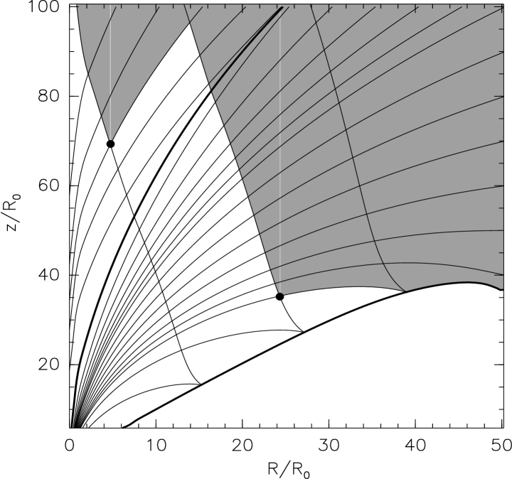
Figure 2: Topology of the characteristics and Mach cones for the final state. The thin lines indicate the two distinct families of characteristics. The lower heavy line indicates the classical fast surface, the upper heavy line the modified-fast surface or limiting characteristic. Two families of characteristics originate from the classical fast surface. For each point in space they spawn the Mach cone, i.e. the area which is causally connected to the origin. The Mach cones originating in the two points indicated by black circles are shown as shaded regions. One Mach cone originates above the modified-fast surface, the other below. The flow is sub-fast magnetosonic in the lower right region; therefore no characteristics exist there and signals can propagate freely.

Figure 3: Evolution of the integrals of motion along a typical fieldline at intermediate latitudes for the final state. The left plot shows, from top to bottom, the integrals angular velocity $\Omega$ (dot-dashed), total energy $E$ (long-dashed), entropy $Q$ (solid), mass- to magnetic flux ratio $\Psi_{A}$ (dotted) and specific angular momentum $L$ (short-dashed) along the fieldline. The curves for entropy and total energy are almost identical. The values of each curve have been normalised to unity near the top boundary. The right plot shows the position of the integral lines and the fieldline in the poloidal plane. The values chosen for the integrals are the same, as the ones for the normalisation in the left plot. The integral lines are almost indistinguishable. The dotted lines indicate the critical surfaces of the final model as in figure 1.

In this section we discuss the results of a particular simulation which shows the properties of a typical run. The model parameters are chosen as $(x,\lambda^{2},\mu,\kappa,\gamma)=(0.75,136.9,2.99,2,1.05)$. This particular model has been discussed in detail in Vlahakis et al. (2000). The simulation evolves for several Alfvénic crossing times, such that the final state can be considered as relaxed.

4.1 Overall relaxation

The initial conditions are not a steady solution of the system of equations under consideration. Therefore, the initial conditions will relax toward a final steady state, if this exists, in accordance with the boundary conditions. These do differ, as discussed in the previous section, from the boundary conditions of the analytical model. So we expect the final numerical state to be different from the analytical, also. Furthermore, the analytical model is not valid near the rotation axis. The numerical model includes the axis consistently, where the initial conditions will likely deviate most from the final state.

As expected from the high MHD signal velocities, the inner regions of the flow evolve very rapidly towards the final state. MHD-waves communicate changes of the inner flow to the outer regions and are clearly visible as bends moving along the fieldlines. After a couple of Alfvénic crossing times, the computational domain does not change substantially anymore and the simulation is halted.

4.2 Critical MHD surfaces and characteristics

A classical MHD critical surface is the location of points where the poloidal velocity $V_{\rm p}$ equals the phase speed of one of the MHD waves propagating along the flow. There are three such surfaces corresponding to the three MHD waves, namely the slow magnetosonic, Alfvén, and fast magnetosonic, with phase speeds $v_{\rm s}$, $v_{\rm Ap}$, and $v_{\rm f}$, respectively. Figure 1 shows the location of the MHD critical surfaces for the initial and the final model. In the initial state the slow magnetosonic surface is located at some distance from the lower boundary; in the final state, it almost disappears bellow the boundary.

The most important of the three MHD surfaces is the fast one, because it is related to the causal connection between the asymptotic part of the flow and the upstream (sub-fast) regime. In the super-fast regime signals can only propagate within a Mach cone around the direction of the poloidal velocity vector. The opening angle of this cone is a function involving the propagation speeds of the MHD waves and the flow speed. The two sides of the cone coincide with the local characteristic curves of the MHD equations. Since the flow speed as well as the MHD wave speeds change from point to point the Mach cone’s opening angle is not constant and the final area to which a signal propagates – and which is causally connected with the origin of the signal – does not resemble a cone, in general, as seen in figure 2. This is similar to the light cone in Penrose diagrams.

Due to the topology of the characteristics near the classical fast surface, a Mach cone with its origin in the super-fast regime of the flow may end on the fast surface, below which a signal may propagate freely. Thus, a signal that originates in the super-fast regime may affect the sub-fast regime. This ceases to be the case downstream from a limiting characteristic, or fast magnetosonic separatrix surface (FMSS), or, modified-fast surface, for short (Bogovalov 1994; Tsinganos et al. 1996). It can be shown that the limiting characteristic coincides with the fast surface only in the case where the poloidal velocity is normal to the latter. The underlying analytical model has a conical modified-fast surface (Vlahakis et al. 2000). The existence and location of this surface is very sensitive to the topology of the magnetic field and thus is easily destroyed when modifying the analytical solution to obtain the initial numerical model and boundary conditions. Still the modified-fast surface is present in the initial model near the axis, as seen in figure 1 as a line at constant angle. While the classical MHD surfaces do not change much away from the boundary, the modified-fast changes its location significantly. As is shown in figure 2, all characteristics converge to the limiting one at both ends, i.e. near the origin and far away from the base of the flow. In the self-similar solution this can be observed only near the origin.

Since the numerical boundaries are not completely transparent to magnetosonic waves, these will artificially influence the solution near the edge of the computational box. This is evident, for example, in the downwards bend of the critical surfaces near the outer $R$ boundary, or possibly even the disappearance of the slow magnetosonic surfaces.

4.3 MHD integrals of motion

It can be shown, that steady, axisymmetric, ideal MHD flows conserve several physical quantities along the fieldlines. This means that these so called integrals of motion are a function of the magnetic flux $A$ only. The integrals are the entropy function $Q$, the mass-to-magnetic-flux ratio $\Psi_{A}$, the total angular velocity $\Omega$, the total specific angular momentum $L$ and the total energy-to-mass flux ratio $E$. These integrals are given as

$$Q=P/\rho^{\gamma},$$ (17)

$$\Psi_{A}=4\pi\frac{\rho V_{\rm p}}{B_{\rm p}},$$ (18)

$$\Omega=\frac{1}{R}\left(V_{\phi}-\frac{B_{\phi}V_{\rm p}}{B_{\rm p}}\right),$$ (19)

$$L=R\left(V_{\phi}-\frac{4\pi}{\mu_{0}}\frac{B_{\phi}}{\Psi_{A}}\right),$$ (20)

$$E=\frac{V^{2}}{2}+\frac{\gamma}{\gamma-1}\frac{P}{\rho}+\Phi-\Omega R\frac{4\pi}{\mu_{0}}\frac{B_{\phi}}{\Psi_{A}}.$$ (21)

Due to the modifications applied to the magnetic field, the fieldlines do not coincide with the integral lines in the initial conditions. During the relaxation process the structure of the flow changes and a realignment can be observed. The realignment is not perfect as seen in the left panel of figure 3, where the values of the integrals are plotted along a typical fieldline at intermediate latitudes. The integrals vary along the fieldline, especially near the base, where they rise (or fall) steeply, before approaching their final value asymptotically. Fieldlines further out show less variation than fieldlines further in.

This means, that the surfaces of the constant values of the integrals are not exactly parallel to the surfaces of constant magnetic flux, and further, that even some of the integrals are not parallel to each other. In fact, only entropy and total energy are perfectly aligned.

There are several possibilities to explain this discrepancy. First, the calculation of the magnetic flux and its iso-surfaces is not accurate enough. This does certainly play a role, since the magnetic field is only interpolated linearly in the calculation of the magnetic flux. Another interpolation of low order is made to calculate the contours. So interpolation errors sum up. To check, the magnetic fieldlines have been calculated with a different method as the streamlines of a mass-less particle flowing through a vector field given by the magnetic field. This shows similar behaviour of the integrals. On the other hand, the relative change of the integrals along the fieldline is only up to 20%, while the integrals change by several orders of magnitude across the fieldlines. So the error in the calculation is actually low, but should still be accounted for. This is clearly illustrated by the right plot in figure 3, which shows the location of all integral lines and the fieldline in the poloidal plane. They are virtually indistinguishable. Fieldlines near to the axis generally show higher miss-alignment than fieldlines further out. The integral lines always match each other almost perfectly.

The next source of potential inaccuracies is the nature of the numerical code NIRVANA. This is a non-conservative, grid-based MHD code. As such it does not guarantee the conservation of energy- or momentum-flux across grid-boundaries down to machine precision level, and leads to numerical dissipation. The degree of numerical dissipation can be estimated by convergence studies – as done by Krause & Camenzind (2001) in the context of jet propagation – which show, that NIRVANA conserves energy and momentum to a reasonable level. Our own calculations at different resolutions confirmed this. Further, very high numerical resistivity would rather lead to an increase of the miss-alignment of the integral lines along the flow instead of an realignment as observed in our simulations.

Most probable is though, that the miss-alignment near the base is due to the mathematically overspecified boundary conditions (e.g. Krasnopolsky et al. 2003).

4.4 Acceleration and collimation

Figure 4: Surfaces of constant conserved total energy $E$ in the poloidal plane for two different energy values. The thin lines show the initial state, while the final state is shown in heavy lines. The dotted lines indicate the critical surfaces as in the previous figures. During the relaxation phase the integral lines and fieldlines reallign. In the final state integral lines are almost perfectly parallel to the magnetic fieldlines.

Figure 5: Evolution of the individual contributions to the total energy $E$ on the integral lines shown in figure 4. Again, thin lines indicate the initial state, while heavy lines the final state. The two clearly separated sets of lines belong, from top to bottom, to the inner and the outer integral line in figure 4. The total energy is shown as solid (also, label E) line, the other line types indicate the different contributions as kinetic energy (dotted/K), enthalpy (dot-dashed/H) and Poynting flux (dashed/P). The gravitational energy is not shown, since it is orders of magnitude lower.

Figure 6: Logarithmically spaced contours of the enclosed poloidal current $B_{\phi}R$ of the final model as solid lines. The dotted lines indicate the MHD critical surfaces as in the previous plots. The absolute current density is highest near the lower left corner. Beyond the modified-fast surface, the current shows a local maximum, before decreasing again sharply towards the axis.

Figure 7: Angle between the flowline and the rotation axis $\delta=\arctan V_{R}/V_{z}$ along the same fieldlines as shown in figure 4. The thin lines show the initial state, while the final state is shown as heavy lines. The upper set of curves corresponds to the outer fieldline, and the lower to the inner.

The contributions to the total energy $E$ are, from left to right in equation (21), the kinetic energy, the enthalpy, the gravitational potential and the Poynting flux. Strictly speaking, all these quantities are energy-to-mass flux ratios, but we will henceforth drop this cumbersome notation and refer to them in this simplified form. Since the total energy is conserved along a fieldline, acceleration of the flow implies an increase of kinetic energy along the fieldline at the expense of other forms of energy. At the base of the fieldline, in the sub-slow region, the kinetic energy will be lower than the Poynting flux or enthalpy, while at the top, where the flow is super-fast magnetosonic, the total energy is dominated completely by the kinetic energy. Thus, along the flow different sources of energy will be transformed into kinetic energy. The dominant conversion channel depends on the position on the fieldline in relation to the critical surfaces. In principle each fieldline passes through all phases. But since the spatial resolution and extent of our simulation box is limitied, we will have to show the different conversion channels on different fieldlines.

Figure 4 shows the integral lines of the total energy for two different values of $E$ for the initial and the final state. We assume for a moment, that the integral line and the fieldline are identical – which is actually close to reality as previously discussed – and limit our interest to the integral lines only. This makes the comparison of initial to final model easier, since the value of the total energy does not change, but we rather jumped from one fieldline to the other. Figure 5 shows the different contributions to the total energy integral (eq. 21) along these fieldlines. At the base of the outer fieldline the Poynting flux dominates over the enthalpy and kinetic energy, the lowest contribution, apart from gravitational energy which is not shown. Along the fieldline the flow gains kinetic energy at the expense of Poynting flux and, to a lesser degree, enthalpy. At the outer boundary of the computational domain, the flow is already kinetically dominated due to acceleration through the Lorentz force. The initial model and the final state look very similar. In the final state the acceleration is slightly more efficient, especially near the base.

Two different mechanisms are responsible for the acceleration. Bellow the Alfvénic surface, the magneto-centrifugal mechanism taps into the rotational energy of the magnetic fieldlines, which are stirred at their base by the underlying accretion flow, and propels the plasma outwards and upwards through centrifugal forces like a bead on the wire (Blandford & Payne 1982; Pelletier & Pudritz 1992). Beyond the Alfvénic surface this mechanism is inefficient. The flow is accelerated instead directly by the gradient of the toroidal magnetic pressure which builds up because of the inertia of the fluid. The energy stored in the tightly bound-up magnetic field loops acts similarly to an uncoiling spring (Uchida & Shibata 1985) and is transfered into kinetic energy of the plasma parcels.

Near the modified-fast surface the flow properties change character. The upper set of curves in figure 5 shows the energy contributions on a fieldline which crosses the modified-fast surface at a height of approximately $70\,R_{0}$. This fieldline is already kinetically dominated at the lower boundary of the computational domain. The acceleration continues until the flow crosses the FMSS. There, kinetic energy is converted back into Poynting flux and the flow slightly decelerates. The equipartion between enthalpy and Poynting flux is coincident and not typical. This change of character of the flow is not seen in the initial state, neither for this particular fieldline, which did not cross the FMSS, nor for fieldlines further in, which do cross the FMSS. The accelaration is not resumed beyond the modified-fast surface.

The collimation process is best understood in terms of poloidal current lines as shown in figure 6 for the final state. The azimuthal magnetic field component $B_{\phi}$ points out of the plane, and the poloidal current $\mbox{\boldmath$j$}_{\rm p}$ flows in the counter-clockwise sense along the indicated current lines. Let’s focus first on the region below the modified-fast surface. In this region all the poloidal current lines close near the equator outside of the simulation box. The poloidal component of the Lorentz force, i.e. $\mbox{\boldmath$j$}_{\rm p}\times\mbox{\boldmath$B$}_{\phi}+\mbox{\boldmath$j$}_{\phi}\times\mbox{\boldmath$B$}_{\rm p}$ points inwards on the “left” side of the current loops and the flow is collimated. We find decollimation on the “right” side of the currents loops, where the first term points outward. However, this region is also affected by the outer boundary and the decollimation may be, at least partly, a numerical artifact.

Beyond the modified-fast surface the enclosed poloidal current $B_{\phi}R$ takes a local maximum. Near the FMSS, the first term of the poloidal Lorentz force points outward, while the second term $\mbox{\boldmath$j$}_{\phi}\times\mbox{\boldmath$B$}_{\rm p}$ is negligible already beyond the Alfvénic surface. The flow decollimates (and decellerates) while crossing the modified-fast surface. After crossing the local maximum in the azimuthal current distribution, i.e. on the falling side of poloidal loops, the collimation is resumed, since both components point inward again. However, the efficiency of collimation lowers continously, since the flowline encounter decreasing absolute values of poloidal current.

A different way to illustrate the collimation is to plot the angle between the poloidal flow lines and the rotation axis $\arctan V_{R}/V_{z}$ as shown in figure 7. Again, we show values along the same fieldlines as in figure 4. In the initial state, and for that matter in the analytical solution, the opening angle steadily decreases along the flow. In the final state, the opening angle increases strongly as the flow crosses the modified-fast surface. Inspection of fieldlines further in, reveals that the collimation is resumed but with low efficiency, as noted before. The opening angle of the outer fieldline increases near the outer boundary. This is, as discussed, most probably an artifact of the outer boundary.

Figure 8: Logarithmically spaced contours of M. The dotted lines indicate the MHD critical surfaces as in the previous plots.

Finally, figure 8 shows the functions M of the analytical solution, calculated from the final numerical state as

$$M_{\rm N}=\left(\frac{\mu_{0}\rho V_{\rm p}^{2}}{B_{\rm p}^{2}}\right)^{1/2}.$$

Note that some minor differences from the conical shape of the analytical function exist only near the outer boundary and beyond the modified-fast surface.

5 Discussion

5.1 Robustness of the model

We found that the results of the numerical simulation presented in this paper are robust. The conclusions do not hold exclusively for the presented numerical model, i.e. initial conditions and boundary conditions. For example, we explicitely performed simulations with very different initial conditions for the computational domain including 1) rotation of the disk starts at $t=0$, i.e. $B_{\phi}=0,V_{\phi}=0$ initially; 2) vertical poloidal magnetic field, i.e. $\mbox{\boldmath$B$}_{\rm p}=B_{z}\mbox{\boldmath$\hat{e}$}_{z}$; 3) vertically non-stratified medium, i.e. $(\rho,P)=f(R,z=0)$; and combinations thereof. The results are qualitatively similar. Small quantitative differences arise through the influence of the downstream boundaries. That means, that the conclusions are independent of the initial conditions as desired. The final state is indeed given only by the propagation of the imposed boundary conditions into the computational domain.

Further, the properties are robust to same changes in the boundary conditions. For example, in this work we imposed the magnetic field component $B_{R}$ from the analytical solution on the lower $z$ boundary, and extrapolated the other from the computational domain under the $\mbox{\boldmath$\nabla$}\!\cdot\!\mbox{\boldmath$B$}$-free constraint. We also performed simulations, where we instead imposed the magnetic flux function $A$ from the analytical solution, with the same qualitative results. We also relaxed the number of boundary conditions to impose (see discussion further down) and obtained similar results. Albeit, we could not reduce the number of boundary conditions to the desired one for numerical reasons specific to this particular profile of the azimuthal vector components on the lower boundary. The aim of this work was, to stay as closely as possible to the analytical model without introducing more differences in the models than necessary.

As discussed in the previous paragraphs, the numerical results are unaffected by certain changes to the initial conditions and the boundary conditions imposed upstream. In the following we will offer some remarks on the influence of the boundary conditions downstream. For numerical reasons we have to provide values for the physical quantities on the downstream boundaries as well. Ideally, these boundaries should be transparent and should not influence the computational domain artificially, since they exist only as numerical boundaries beyond which the numerical code does not solve the equations; they are not related to real physical boundaries in any way.

One way to judge the possible impact of numerical boundaries is to study the behaviour of MHD waves propagating through the boundary. Again, ideally, the waves should propagate unhindered and no part should be reflected. Although the numerical code we use does not take special measures to inhibit the reflection of waves, numerical experiments show, that in a super-fast magnetosonic situation, no magnetosonic waves are reflected at all. In the sub-slow regime, all waves may be reflected partially, but the amplitude of the reflected wave is in general very low compared to the incident. We note further, that the reflected waves propagate, if at all, only in accordance with their respective Mach cones. No artificial propagation of waves along the boundary is observed. Due to the topology of the Mach cone in our model (see figure 2), this means, that no wave traversing the upper $z$ boundary can propagate back into the computational domain and influence it. The same is true for the upper $R$ boundary beyond the intersection with the classical fast surface. In summary, only the upper $R$ boundary below the classical fast surface can affect the computational domain.

As a side note we remark, that due to the shape of the Mach cone, most of the classical super-fast region cannot influence the sub-slow region, also, since the Mach cone intersects the classical fast surface only outside of the computational box. In fact, only points below the characteristic, which originates at the intersection of the upper $R$ boundary and the classical fast surface have Mach cones which reach into the sub-fast region within the computational domain. The Mach cones originating in points above this characteristic do not reach into the sub-fast region before encountering the outer boundaries.

Another aspect to consider is the number of boundary conditions to impose at the upstream boundary. Following Bogovalov (1997), the number of boundary conditions is to be reduced by one for each outgoing wave propagating perpendicular to the boundary. In the present work, we over-specified the lower $z$ boundary, i.e. we imposed more conditions than mathematically allowed, even if one does not take into account the ambiguity with regard to the nature of the critical surfaces. We chose to do so mainly for technical reasons specific to this particular model, as discussed elsewhere in this paper. The only artifact that we may attribute to the over-specification of the launching-surface, is the steep increase (decrease) of the integrals near the base of the fieldlines, see figure 3, where the flow tries to match the integral lines given by the conditions at the critical surfaces to the conditions imposed artificially on the boundary. See also Krasnopolsky et al. (2003) on the risk of creating discontinuities by over-specification of the boundary conditions. We note however, that the implementation of a relaxed number of boundary conditions has been tested successfully with other models, and will be presented and used in future work.

5.2 Comparison to related studies

In general, the analytical solution (Vlahakis et al. 2000) and our numerical solution are quite similar, as expected from the way the latter is constructed. Differences arise only where the self-similarity assumption is violated. We explicitly included the rotation axis into our analysis. There the flow properties are mainly given by the symmetry conditions on the axis, which are not compatible with radial self-similarity, in general, due to their diverging behaviour. In our numerical model all physical quantities match their finite value on the axis smoothly. The numerical model solves the problem of the termination of most radially self-similar analytical solutions at finite distance along the flow. In particular, the $R$-component of the flow velocity decreases continously and eventually becomes negative. At larger distances, even the $z$-component changes sign as well. So, technically the solution does not extent to infinity, but terminates at finite distance along the flow. This behaviour is not present in the numerical model. Neither do the fieldlines bend inwards, nor would this automatically mean, that the flow terminates at the axis, since the azimuthal magnetic field component $B_{\phi}$ vanishes at the axis and the Lorentz force does likewise.

The only region where substantial difference arise is near the modified-fast surface. At this surface the flow just looses causal contact with the base for the analytical model, but no locally evaluated quantity behaves differently than before crossing this surface. This is not the case in the numerical model. Again, the flow looses causal contact with the base, but unlike the analytical solution, in some way it also looses its memory of the flow properties. In fact, all relevant physical quantities change at the critical surface and find a new equilibrium value. On the other hand, there is no shock present either. In principle a terminated solution can connect to infinity by going through a shock beyond the critical surface. This does not seem to be the case here, since, although all physical quantities change noticeably, the involved gradients are moderate. The behaviour of the flow near the modified-fast surface is closely related to the presence of a local maximum in the enclosed poloidal current distribution further down the flow. This temporarily reverses the direction of the dominant part of the Lorentz force $\mbox{\boldmath$j$}_{\rm p}\times\mbox{\boldmath$B$}_{\phi}$ and therefore decelerates and decollimates the flow noticeably. It remains to be checked if this is a general behaviour of solutions crossing the modified-fast surface.

One qualitative difference between our model and Krasnopolsky et al. (1999) the shape of fast magnetosonic surface. In our case the flow is classically super-fast magnetosonic everywhere near the axis, in fact even on part of the launching surface. In contrast, the axial region in Krasnopolsky et al. (1999, 2003) is occupied by a cold, light, sub-fast magnetosonic flow injected at the lower boundary, apparently for numerical reasons. Further, our model crosses not only the classical, but also the modified-fast surface. The structure of the magnetic field is very similar, only after crossing the FMSS, does the magnetic field tend to open up. This is neither described elsewhere, nor is it understood so far and will be the subject of further investigations.

By extrapolating the experience we obtained in this study, the shape of the Mach cones originating from the downstream boundaries may influence the solution in the computational domain, since these boundaries may still be in causal contact with the base of the flow. This might explain the sensitivity of Krasnopolsky et al. and others model to changes of the computational box size – a problem that we did not encounter (see for example Ustyugova et al. 1995, for a discussion). A direct consequence of the shape of the super-fast surface is the fact, that our models reach higher fast-Mach numbers $M_{\rm f}$ – typically $\sim 5$ at the upper boundary and in excess of $10$ near the axis – and therefore the flow is more efficiently accelerated. On the other hand a high poloidal magnetic field strength at the axis, i.e. low Mach numbers, seems to stabilise the flow against non-axisymmetric Kelvin-Helmholtz instabilities as discussed by Ouyed et al. (2003) and more generally by Appl & Camenzind (1992), Baty (2005) and references therein. The mass-loading is however given by the conditions on the launching surface as Krasnopolsky et al. (2003) showed very convincingly.

Recently, Casse & Keppens (2004) studied resistive MHD accretion flows threaded by a vertical magnetic field and achieved near-steady state outflows along the axis. Their analysis includes the accretion flow dynamics and does not rely on assumed ad-hoc boundary conditions for the disk at a launching surface. Similar to our model and unlike Krasnopolsky et al. (1999), the axial region is not taken by an artificial cold axial jet but rather self-consistently by a hot outflow. This allows the outflow to cross the classical fast surface even on the axis. However, it is not clear whether it also crosses the modified-fast surface and what the structure of the characteristics is. Further, the enthalpy flux seems to play a important role at the base of the flow, while our model is Poynting flux dominated at the base and shows very high accelerations efficiency along the outflow.

5.3 Conclusions and future plans

In this paper, we verified the analytical model presented by Vlahakis et al. (2000) with numerical methods. Further, we extended the analysis into the domain where the analytical model breaks down due to the self-similarity assumption, i.e. we included the rotation axis in a self-consistent way. Unlike the analytical solution, our numerical solution is a global one in the sense, that it is not terminated but extends – given enough computational resources and infinite computational box size – to infinity. We confirmed the properties of the analytical solution in its domain of availability, in particular the existence of the modified-fast surface or fast magnetosonic separatrix surface. The numerical solution shows different properties near and beyond the modified-fast surface, where the flow changes character. This change of character manifests itself in the appearance of a further local maximum in the enclosed poloidal current beyond the modified-fast surface, which is responsible for a temporary deceleration and decollimation of the flow.

This work is intended to be the first in a series of papers. We will subsequently address some of the shortcomings of this work by lovering the launching surface down to the equator and applying only the neccesary number of boundary conditions. In this way it will be possible to explore a wide range of scenarios for the jet-launching surface.

References

- Appl & Camenzind (1992) Appl S., Camenzind M., 1992, Astronomy and Astrophysics, 256, 354
- Baty (2005) Baty H., 2005, Astronomy and Astrophysics, 430, 9
- Blandford & Payne (1982) Blandford R. D., Payne D. G., 1982, MNRAS, 199, 883
- Bogovalov (1994) Bogovalov S. V., 1994, MNRAS, 270, 721
- Bogovalov (1997) Bogovalov S. V., 1997, Astronomy and Astrophysics, 323, 634
- Casse & Keppens (2004) Casse F., Keppens R., 2004, The Astrophysical Journal, 601, 90
- Hartigan et al. (1995) Hartigan P., Edwards S., Ghandour L., 1995, The Astrophysical Journal, 452, 736
- Königl & Pudritz (2000) Königl A., Pudritz R. E., 2000, Protostars and Planets IV, p. 759
- Krasnopolsky et al. (1999) Krasnopolsky R., Li Z., Blandford R., 1999, The Astrophysical Journal, 526, 631
- Krasnopolsky et al. (2003) Krasnopolsky R., Li Z., Blandford R. D., 2003, The Astrophysical Journal, 595, 631
- Krause & Camenzind (2001) Krause M., Camenzind M., 2001, Astronomy and Astrophysics, 380, 789
- Lada (1985) Lada C. J., 1985, Annual Review of Astronomy and Astrophysics, 23, 267
- Nakamura & Meier (2004) Nakamura M., Meier D. L., 2004, The Astrophysical Journal, 617, 123
- Ouyed et al. (2003) Ouyed R., Clarke D. A., Pudritz R. E., 2003, The Astrophysical Journal, 582, 292
- Pelletier & Pudritz (1992) Pelletier G., Pudritz R. E., 1992, The Astrophysical Journal, 394, 117
- Sauty & Tsinganos (1994) Sauty C., Tsinganos K., 1994, Astronomy and Astrophysics, 287, 893
- Tsinganos et al. (1996) Tsinganos K., Sauty C., Surlantzis G., Trussoni E., Contopoulos J., 1996, MNRAS, 283, 811
- Uchida & Shibata (1985) Uchida Y., Shibata K., 1985, Publ. of the Astronomical Society of Japan, 37, 515
- Ustyugova et al. (1995) Ustyugova G. V., Koldoba A. V., Romanova M. M., Chechetkin V. M., Lovelace R. V. E., 1995, The Astrophysical Journal Letters, 439, L39
- Vlahakis & Tsinganos (1998) Vlahakis N., Tsinganos K., 1998, MNRAS, 298, 777
- Vlahakis et al. (2000) Vlahakis N., Tsinganos K., Sauty C., Trussoni E., 2000, MNRAS, 318, 417
- Ziegler (1998) Ziegler U., 1998, Computer Physics Communications, 109, 111