A Sudden Gravitational Transition

Abstract

We investigate the properties of a cosmological scenario which undergoes a gravitational phase transition at late times. In this scenario, the Universe evolves according to general relativity in the standard, hot Big Bang picture until a redshift $z\lesssim 1$. Non-perturbative phenomena associated with a minimally-coupled scalar field catalyzes a transition, whereby an order parameter consisting of curvature quantities such as $R^{2},\,R_{ab}R^{ab},\,R_{abcd}R^{abcd}$ acquires a constant expectation value. The ensuing cosmic acceleration appears driven by a dark-energy component with an equation-of-state $w<-1$. We evaluate the constraints from type 1a supernovae, the cosmic microwave background, and other cosmological observations. We find that a range of models making a sharp transition to cosmic acceleration are consistent with observations.

Introduction. The observational evidence for a low density, spatially-flat, accelerating Universe poses a severe challenge to theoretical physics. Solutions which have been proposed include a cosmological constant, an ultra-light scalar field, and modifications to Einstein’s gravity. An approach which unifies these different viewpoints can be found in Sakharov’s description of the gravitational physics of the vacuum Sakharov:1967pk . According to his proposal, quantum effects of the particles and fields present in the Universe give rise to the cosmological constant and gravitation itself. Although this approach has not solved the problem of the cosmological constant, it has pointed the way towards a novel model for the dark energy.

Quantum effects of an ultra-light, minimally-coupled scalar field have been proposed to account for the dark energy phenomena in the vacuum metamorphosis scenario Parker:1999td ; Parker:1999ac ; Parker:2000pr ; Parker:2001 ; Parker:2004 . Effectively, the Ricci scalar curvature serves as an order parameter, marking a gravitational transition when it drops to the value $\chi m^{2}$. Here, $m\sim 10^{-33}$ eV is the mass of the scalar field and $\chi$ is a numerical constant of order unity which is set by the theory. For most of the history of the Universe, up until $z\sim 1$, $R>\chi m^{2}$ and the vacuum stress-energy is negligble. Since the local value of the Ricci scalar exceeds this critical value in the vicinity of galaxies today, we see no vacuum energy nearby. On the largest scales, however, the vacuum term comes to dominate the cosmic evolution as $R\to\chi m^{2}$. A detailed analysis shows that feedback from the vacuum prevents $R$ from evolving past the critical value, in a sort of gravitational Lenz’ law which maintains $R=\chi m^{2}$ Parker:2004 . The ensuing, large-scale cosmic expansion begins to accelerate, driven by a dark energy component with an equation-of-state $w<-1$ which approaches $-1$ in the future.

Despite the sharp change in the character of gravitation, we are still justified to use basic cosmological tools such as the luminosity distance. Although the transition changes the relationship between curvature and matter, we still have a metric theory and a complete description of the evolution of the expansion scale factor.

The vacuum metamorphosis scenario is distinct from scalar-tensor theories of gravity Yasunori or high-energy physics inspired modifications of the gravitational action whereby the Einstein-Hilbert action is replaced by a function of the Ricci scalar, $-16\pi G{\cal L}_{g}=R\to f(R)$. (See Ref. Carroll:2003wy for a recent example.) In our case, the gravitational action is modified by vacuum polarization effects of the matter content in the theory. However, the modifications include contributions from $R,\,R_{ab},\,R_{abcd}$ so there is not a simple way to re-express the model in terms of an equivalent, non-minimally-coupled scalar field. (See Refs. Teyssandier:1983 ; Wands:1993uu for a discussion of the equivalence between higher-order gravity theories and scalar-tensor gravity.) Furthermore, the scenario we consider is different from other dark energy models based on curved-space quantum field theory effects Sahni:1998at ; Onemli:2004mb , in that the cosmic acceleration arises from non-linear, non-perturbative phenomena. In fact, the theory we examine in this article is similar in spirit to the gravitational transition investigated by Tkachev Tkachev:1992an . The distinction here is in the form of the vacuum stress-energy, which is based on the novel results by one of us and collaborators Parker:1999td ; Parker:1999ac ; Parker:2000pr ; Parker:2001 ; Parker:2004 . The one-loop effective action, which is complete for a free massive scalar field in curved spacetime, can be viewed perturbatively in terms of Feynman diagrams. Classical gravitons attach to the vacuum loops of the scalar field. With increasing number of external gravitons, these diagrams require counterterms that give rise to renormalization of the cosmological constant, Newton’s constant, and several other constants that appear in terms that are of second order in the Riemann tensor. In the limit of a massless field, the conformal trace anomaly arises from finite parts of the second order terms and does not depend on the values of the renormalized constants. The terms in the perturbative expansion that are of still higher order in the Riemann tensor have no infinities and appear to be relevant only at Planckian scales. However, summation of an infinite subset of those terms shows that they may give rise to a large nonperturbative effect when the Ricci scalar curvature approaches a specific value proportional to the square of the scalar particle’s mass. Alternatively, the functional integral over fluctuations of the scalar field in the one-loop effective action can be performed and the result can be expressed in terms of the exact heat kernel of the scalar field equation. By studying known exact solutions for the heat kernel, one can infer a plausible asymptotic form of the heat kernel and show that it leads to the same type of large nonperturbative effect when the Ricci scalar curvature approaches a value, $\chi m^{2}$, proportional to the square of the particle’s mass. This latter approach does not rely on a subset of Feynman diagrams and is thus fully nonperturbative. Like the conformal trace anomaly, this effect is independent of the values of renormalized constants. If the calculation is valid, vacuum metamorphosis must occur if the universe contains a light scalar field with $\chi$ positive. Since a complete description of the stress-energy tensor source for Einstein’s equations must include all matter fields as well as vacuum stress-energy, the cosmological phenomena resulting from the vacuum stress-energy is inevitable given the existence of such a scalar field.

The original vacuum metamorphosis model is tightly constrained, although not eliminated, by observations Parker:2003 ; Komp:2004 . We find the basic behavior to be of sufficient interest to justify further investigation. In this article we speculate that other curvature quantities such as $R_{ab}R^{ab}$ or $R_{abcd}R^{abcd}$ can serve a similar role as order parameters for a gravitational transition. In the following we examine the cosmic evolution resulting from such gravitational transitions. We evaluate the observational constraints based on type 1a supernovae, the cosmic microwave background, the Hubble constant, and large scale structure. We stop short of making a full perturbation analysis — the detailed equations require a lengthy investigation — and we regard this as a first cut at a family of models extending the vacuum metamorphosis scenario.

Gravitational Transition. In the vacuum metamorphosis scenario, non-perturbative effects of a light scalar field lead to a gravitational transition when the Ricci scalar reaches the level $R={\bar{m}}^{2}$. Here we absorb the dimensionless parameter $\chi$ into the mass $\bar{m}$. Before the transition, the cosmic evolution is determined by the standard FRW equation

$$3H^{2}=8\pi G\rho_{m}\qquad a<a_{*}$$ (1)

where $a_{*}$ marks the time of the transition, and $\rho_{m}$ represents all matter and radiation. There is no need to include the vacuum energy density, $\rho_{v}$, since it is negligible at these early times. After the transition, however, the cosmic evolution is given by

$$R=6(\dot{H}+2H^{2})={\bar{m}}^{2}\qquad a\geq a_{*}\,.$$ (2)

Notably, the subsequent evolution of matter and radiation after the transition have no influence on the expansion rate. The vacuum energy does not merely contribute to the cosmic energy density driving the expansion, as for most dark energy models. Rather, it changes the form of gravity on cosmological scales and completely determines the expansion. After solving (2) for $H(a)$ or $a(t)$, however, we can still use the standard FRW equation

$$3H^{2}=8\pi G\left(\rho_{m}+\rho_{v}\right)$$ (3)

together with the evolution of the matter density parameter

$$\Omega_{m}(a)=\left(\frac{H_{*}}{H}\right)^{2}\left(\frac{a_{*}}{a}\right)^{3}\,,$$ (4)

to deduce the properties of an equivalent dark energy that has the equation-of-state, $w=p_{v}/\rho_{v}$:

$$w=-\left(1+\frac{2}{3}{\dot{H}/H^{2}}\right)/\left(1-\Omega_{m}(a)\right).$$ (5)

The inferred equation-of-state is super-negative, with $w<-1$ which approaches $w\to-1$ in the future. For this model, there is a single free parameter, $\bar{m}$. So, after choosing a present day Hubble constant $H_{0}$, the value of $\bar{m}$ determines the matter density:

$$\Omega_{m}|_{0}=\frac{2\sqrt{2}}{3}\left(\frac{\bar{m}}{H_{0}}\right)^{2}\left[\left(\frac{H_{0}}{\bar{m}}\right)^{2}-\frac{1}{12}\right]^{3/4}\,.$$ (6)

The Hubble constant at the time of the transition is $H_{*}=\bar{m}/\sqrt{3}$, so

$$H(a)=\frac{\bar{m}}{2\sqrt{3}}\left[3\left(\frac{a_{*}}{a}\right)^{4}+1\right]^{1/2}$$ (7)

gives the analytic solution to the evolution equation (2). Note that the total energy density and pressure is always positive: $\rho+p=\bar{m}^{2}(a_{*}/a)^{4}/8\pi G$. There is no “big rip” in this scenario Caldwell:2003vq , as the late-time evolution resembles a comological constant-dominated universe.

We propose to extend this gravitational transition model, using $R_{ab}R^{ab}$ or $R_{abcd}R^{abcd}$ as the order parameter in place of $R$. In either case, the evolution before the transition is determined by the standard FRW equation (1). After the transition, from the constancy of the order parameter we have

$$\alpha\left[\dot{H}^{2}+N(\dot{H}H^{2}+H^{4})\right]=\bar{m}^{4}\qquad a\geq a_{*}$$ (8)

where $\alpha=12$ and $N=2,\,3$ for the Riemann and Ricci tensors, and $\alpha=36,\,N=4$ for the Ricci scalar. Linear combinations of these curvature terms which lead to cosmic acceleration, $\ddot{a}>0$, correspond to $3/2<N\leq 9/2$. We can solve these equations numerically to determine the subsequent evolution.

The cosmic evolution under various gravitational transition scenarios is shown in Figures 1,2,3. The hallmark of these models is a rapidly-evolving equation-of-state with $w<-1$. We can see that by decreasing $N$, or increasing the rank of the curvature quantities used to form the order parameter, the strength of the vacuum energy increases. The total $\rho+p$ drops faster in time, and the onset of cosmic acceleration is sharper.

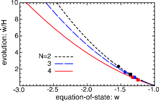
Figure 1: The evolution of the gravitational transition model in the $w-\dot{w}/H$ phase plane is shown. For a given $N$, the model trajectory follows the curve indicated with $\Omega_{m}$ decreasing as the phase variables evolve from the starting point at $(w,\,\dot{w}/H)=(-\infty,\infty)$ and head towards $(-1,0)$. The values corresponding to $\Omega_{m}=0.3,\,0.4$ are indicated by the small squares and circles, respectively. In the case $\Omega_{m}=0.4$ today, $(w,\dot{w}/H)=(-1.55,2.4),\,(-1.45,1.6),\,(-1.35,1.0)$, with the transition occuring at $a_{*}/a_{0}=0.7,\,0.6,\ 0.5$ for $N=2,\,3,\,4$ respectively.

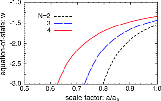
Figure 2: The evolution of the equation-of-state $w$ as a function of the scale factor $a$ is shown. All models have $\Omega_{m}=0.4$ today. For decreasing $N$, the effective gravitational repulsion of the dark energy as measured by $w$ increases. The $N=4$ model is consistent with all observations, the $N=3$ is on the border, and $N=2$ is excluded.

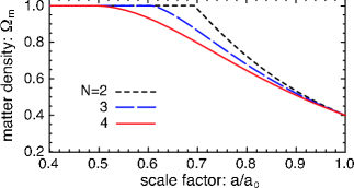
Figure 3: The evolution of the density parameter $\Omega_{m}$ as a function of the scale factor $a$ is shown. All models have $\Omega_{m}=0.4$ today. The matter density drops suddenly at the onset of the transition. The sharpness of the drop grows with decreasing $N$. The $N=4$ model is consistent with all observations, the $N=3$ is on the border, and $N=2$ is excluded.

Another possibility that comes to mind as an order parameter is the Gauss-Bonnet invariant,

$$Q=R^{2}-4R_{ab}R^{ab}+R_{abcd}R^{abcd}.$$ (9)

However, the deceleration parameter $q\equiv-a\ddot{a}/\dot{a}^{2}$ is proportional to the Gauss-Bonnet invariant, $q=-Q/24H^{4}$. This means the curvature cannot evolve down to some constant $Q$ to signal a gravitational transition to cosmic acceleration: $Q<0$ in a matter-dominated universe, but $Q>0$ is required for acceleration.

Constraints. We now consider the observational constraints on the cosmic evolution resulting from the family of generalized vacuum metamorphosis models. These constraints are due to: 1) distance - redshift relationship using type 1a supernovae (SNe) Riess:2004nr ; Knop:2003iy ; 2) the distance to the cosmic microwave background (CMB) last scattering surface and the density $\Omega_{m}h^{2}$ implied by the WMAP measurements Spergel:2003cb ; 3) the Hubble constant based on the HST key project Freedman:2000cf ; 4) the mass power spectrum shape parameter $\Gamma\equiv\Omega_{m}h$ Percival:2001hw ; Pope:2004cc .

• For the SNe we use the 156 supernova, “gold” data set of Riess et al Riess:2004nr and the 54 supernova set of Knop et al Knop:2003iy . We make a simple $\chi^{2}$ test to determine the $2\sigma$ region allowed for each data set.

• For the CMB we exploit the geometric degeneracy of CDM-family models with identical primordial perturbation spectra, matter content at last scattering, and comoving distance to the surface of last scattering Zaldarriaga:1997ch ; Bond:1997wr ; Efstathiou:1998xx . This means that there is a family of dark energy models with different equation-of-state histories and dark energy abundances but essentially identical CMB spectra Huey:1998se . Hence, our best-fitting models are those which are degenerate with the best-fitting $\Lambda$CDM models obtained by WMAP Spergel:2003cb . We have taken the $2\sigma$ $\Lambda$CDM models based on a 5-parameter fit ($\Omega_{\Lambda},\,\Omega_{c}h^{2},\,\Omega_{b}h^{2},\,h,\,n_{s}$ obtained from a combination of earlier work Caldwell:2003hz , new calculations using CMBfast Seljak:1996is , and CMBfit Sandvik:2003ii ). We also use the Big Bang Nucelosynthesis prior $\Omega_{b}h^{2}=0.02\pm 0.002\,(95\%)$ Burles:2000zk . Ultimately, these points in the $\Lambda$CDM $\Omega_{m}-H_{0}$ plane are mapped to points in the VCDM $\Omega_{m}-H_{0}$ plane by fixing the quantities $\Omega_{m}h^{2}$ and the luminosity distance to the last scattering surface. This procedure overlooks differences in the large-angle anisotropy pattern, which would require a full treatment of the cosmological perturbations after the transition to model accurately. However, the $\chi^{2}$ fit between the theoretical model and experiment is dominated by the small-angle anisotropy pattern so these differences should be small. (A preliminary treatment of the large-angle CMB anisotropy suggests the VCDM constraint region shifts to higher $\Omega_{m}$ by $\lesssim 10\%$ Komp:2004 .)

• For the Hubble constant, we require that the value of $H_{0}$ falls within $2\sigma$ of HST’s result $72\pm 8$ km/s/Mpc ($1\sigma$) Freedman:2000cf .

• For the shape parameter, the chief obstacle in applying the 2dF and SDSS results is the difference in the rate of growth of linear density perturbations between our models and a $\Lambda$CDM cosmology. We expect linear perturbation growth to cease at the transition, although we postpone a detailed treatment for a future investigation. The current $1\sigma$ bound on $\Gamma$ has a $\sim 20\%$ uncertainty which should be comparable to the differences resulting from the perturbation growth. For safe margin, we require that our best-fit model has a shape parameter which falls within $3\sigma$ of the bound $\Gamma=0.2\pm 0.03~{}(1\sigma)$ Percival:2001hw ; Pope:2004cc .

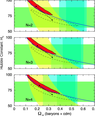
Figure 4: The observational constraints on the $\Omega_{m}-H_{0}$ parameter space for the $N=2,\,3,\,4$ gravitational transition models are shown. The red-filled contour is the WMAP CMB $2\sigma$ region, obtained from the $\Lambda$CDM $2\sigma$ region, given by the black dashed contour, by using the geometric degeneracy. The line connecting the black dots shows the mapping of the best-fit $\Lambda$CDM model to the gravitational transition model. The SN $2\sigma$ regions are shown by the wide, pale blue (Knop et al 2004) and narrow, pale grey (Riess et al 2004) bands. The shape parameter $\Gamma$ $3\sigma$ region is shown by the yellow swath. The Hubble constant $2\sigma$ region is the horizontal green band. For reference, gravitational transition models with age $13.5$ Gyrs lie along the thin blue line. There is significant overlap amongst all model constraints for the cases $N=4$ for the $R^{2}$ transition. Sharper transitions, corresponding to $N<4$, are in conflict with some or all of the observations.

The results are shown in Figure 4. We see that the gravitational transition models require a lower matter density than $\Lambda$CDM to satisfy the CMB constraints, and a higher matter density to satisfy the SN constraints. The $\chi^{2}$ fit to the CMB data for the best-fit model is identical to that for the best-fit $\Lambda$CDM model, due to the geometric degeneracy. The fit to the SN data is marginally better than $\Lambda$CDM ($\chi^{2}=175$ for $156$ SNe Riess:2004nr ; $\chi^{2}=59$ for $54$ SNe Knop:2003iy ). For $N=4$, the original VCDM model, there are viable models near $\Omega_{m}=0.4,\,H_{0}=70$ whereby the transition redshift is $z_{*}\sim 1$ Komp:2004 . However, as $N$ decreases, the tension between CMB and SN data builds. Hence, sharpening the gravitational transition relative to VCDM conflicts with observation. As $N$ approaches $9/2$ it turns out that the gap between the SN and CMB parameter ranges decreases. But in this limit, for fixed matter density today, the transition occurs at earlier and earlier times, at $z_{*}\gg 1$. Since linear perturbation growth is expected to slow or cease at the transition, such an early transition can be expected to wreck the basic structure formation scenario.

There are some straightforward ways to ease the conflict between these gravitational transition models and observations: 1) allow for a small amount of spatial curvature; 2) include the energy of the scalar field itself.

Adding negative spatial curvature improves the fit to the SN data while lowering the matter density. However, the viable CMB region shifts to an even lower range of $\Omega_{m}$, and so the two major constraints remain in conflict. Adding positive spatial curvature, thereby closing the Universe, brings the $2\sigma$ SN and CMB regions into closer agreement. As illustrated in Fig. 5, the addition of a small amount of positive spatial curvature, $\Omega_{k}=-0.05$ at the transition, leads to concordance. The quality of the improvement is best for $N=4$, whereby $\Omega_{m}\approx 0.4$ and $H_{0}\approx 60$ km/s/Mpc lies within the $2\sigma$ contour for all the constraints. Yet, we view the addition of spatial curvature as extraneous. It is unrelated to the mechanism of vacuum metamorphosis or gravitational transition, and there is no direct observational evidence which requires it. Hence, we do not pursue spatial curvature any further.

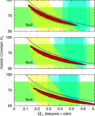
Figure 5: Same as Fig. 4 but with positive spatial curvature. In all cases $\Omega_{k}=-0.05$ and $\Omega_{m}=1.05$ at the time of the transition. The agreement with CMB and SN constraints improves significantly, particularly for the N=4 case as the CMB best-fit point falls inside the $2\sigma$ contour for all other constraints.

Including the energy of the scalar field itself can also bring the SN and CMB constraint regions into better agreement. Here it is necessary to explain that the vacuum stress-energy which gives rise to the gravitational transition consists of the gravitational corrections to the scalar field stress-energy in the state in which the vacuum expectation value of the scalar field is zero. A non-zero vacuum expectation value would contribute the same stress-energy as a free classical scalar field of mass $m$.

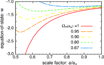
Figure 6: The evolution of the equation-of-state $w$ as a function of the scale factor $a$ is shown for the $N=4$ model including the classical scalar field. In all cases, $w$ starts at $-1$ at the transition, drops below, and then ultimately evolves back to $-1$ in the asymptotic future. For $\Omega_{m}=0.3$ today, only the top curve, with $\Omega_{m}=0.67$ at the transition, produces a viable cosmology satisfying all observational constraints.

This classical scalar field introduces new degrees of freedom into the model. The mass of the scalar field, with potential $V=\frac{1}{2}m^{2}\phi^{2}$, is related by $m^{2}=\bar{m}^{2}/\chi$ to the parameter $\bar{m}$ that determines the cosmological evolution after the transition. Using the value $\chi=6$ suggested by earlier versions of the VCDM model Parker:1999td , then $m^{2}=\bar{m}^{2}/6$. The evolution of such a light field will be strongly damped by the cosmic expansion up to the time of the transition, so that to first approximation it will look like a cosmological constant. In order to contribute a fraction $1-\Omega_{m}(a_{*})$ of the total cosmic energy density at the transition time, the field amplitude must be $\phi=\sqrt{3(1-\Omega_{m}(a_{*}))/2\pi}M_{P}$ where $M_{P}$ is the Planck mass. This is a potential sticking point for the model, much as for scalar field quintessence, since such a high field amplitude should be susceptible to quantum gravitational effects which, for example, induce couplings to all other matter fields. However, the absence of non-gravitational interactions for $\phi$, together with its very small mass $m$, appear to suppress such couplings. Also, one may question whether it is necessary or economical to introduce a second form of dark energy. This reduces to the question of the vacuum expectation value of the field, which must be determined by the initial conditions or perhaps post-inflationary physics. Whether or not the vacuum expectation value is large, for the quantum scalar field that we have been considering, the quantum effects that lead to vacuum metamorphosis are inevitable.

Including an effective cosmological constant before the transition, the evolution equations for the Hubble expansion rate or the scale factor are the same as (8), but with different initial conditions at the transition. For the $R^{2}$ case with $N=4$, the analytic solution is

$$H(a) = \frac{\bar{m}}{2\sqrt{3}}\left[\frac{3\Omega_{m}(a_{*})}{4-3\Omega_{m}(a_{*})}\left(\frac{a_{*}}{a}\right)^{4}+1\right]^{1/2},$$ (10)

$$\Omega_{m}(a) = \Omega_{m}(a_{*})\left(\frac{H_{*}}{H}\right)^{2}\left(\frac{a_{*}}{a}\right)^{3}\,.$$ (11)

The equation-of-state is still obtained from (5). But whereas $w$ is undefined at the transition in the absence of the classical scalar field, now $w(a_{*})=-1$ as illustrated in Figure 6. Also, note that $\Omega_{m}(a_{*})\geq\Omega_{m}(a_{0})$. In the $N=4$ model with $\Omega_{m}(a_{*})=2/3$ and $\Omega_{m}(a_{0})=0.3$, the transition occurs at $a_{*}/a_{0}=0.64$ and the equation-of-state is $w=-1.15$ today. As $\Omega_{m}(a_{*})$ is lowered, the onset of cosmic acceleration is earlier but the transition is later, for fixed $\Omega_{m}(a_{0})$. In the limit that $\Omega_{m}(a_{*})=\Omega_{m}(a_{0})$ the transition occurs at $z_{*}=0$ and the model is equivalent to $\Lambda$CDM.

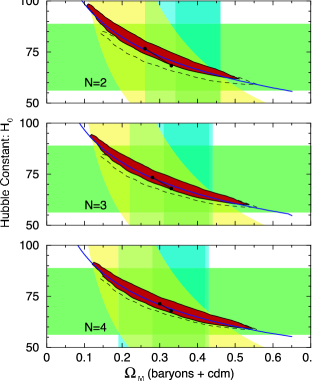
Figure 7: Same as Fig. 4, but the classical mode of the scalar field contributes an effective cosmological constant before the gravitational transition. At the transition, $\Omega_{m}(a_{*})=2/3,\,\Omega_{\Lambda}(a_{*})=1/3$. The result is that the transition to acceleration is softened, and the tension between the CMB and SN constraints is relaxed. Models with $N=2-4$ are viable.

We have evaluated observational constraints for the $R^{2},\,R_{ab}R^{ab}$ and $R_{abcd}R^{abcd}$ models with a cosmological constant. As more $\Lambda$ is added before the transition, the gap between the CMB and SN constraints reduces. In Figure 7 we show the constraints resulting for the case $\Omega_{m}(a_{*})=2/3$. The quality of the $\chi^{2}$ fit to the CMB and SN data are approximately the same as for the cases without the addition of the scalar field contribution. In all cases shown there are viable models near $\Omega_{m}=0.3$ and $H_{0}=70$, providing good motivation for further investigation of these models.

Cosmological Perturbations. The vacuum metamorphosis scenario and its generalizations have dramatic implications for gravitation. The transition occurs when the order parameter, $R^{2}$ in the $N=4$ case, reaches a critical value. On large scales, when the cosmological curvature drops to $R=\bar{m}^{2}$ the transition takes place. On sub-horizon scales, on the scales of voids, this critical value is reached a bit earlier than on average; on the scale of clusters, this value is reached a bit later. Since $R=8\pi G(\rho+3p)$ in Einstein’s gravitation, a high density or pressure will keep $R$ above the critical value. Inside a cluster and on the scale of galaxies, where the mean density is well above the cosmic background, the transition never takes place.

What happens to gravitation after the transition? The field equations become higher-order, so that a static potential obeys a fourth order equation, $(-A\nabla^{2}\nabla^{2}+\nabla^{2})\Phi=4\pi BG\rho$. $\sqrt{A}$ is a length, below which the potential is exponentially suppressed. $B$ modifies the strength of gravity, and grows tiny upon the transition. This would look like a disaster, except that the transition takes place only on large scales, where this Newtonian analysis is invalid.

To treat the scenario in cosmological perturbation theory, we first observe that the gravitational transition takes place on a spacelike hypersurface of constant curvature. And the duration of the transition is effectively instantaneous, based on a numerical modeling of the vacuum effects Parker:2004 . Taking into account small cosmological perturbations, this surface will be a surface of constant $R+\delta R$ to linear order. At times after the transition, the feedback of the vacuum effects on the gravitational field equations forces $R$ to a constant. It is reasonable to surmise that fluctuations $\delta R$ are forced to vanish. To deal with the evolution of fluctuations across the transition we resort to junction conditions, ensuring energy and momentum flow is continuous. Following Ref. Deruelle:1995kd , we can choose a gauge and then match the perturbation variables from pre- to post-transition. In general, we can expect that the pure growing mode which dominates the evolution before the transition will give way to a linear combination of growing and decaying modes afterwards. The evolution of the perturbations after the transition, however, presents a challenge.

If the transition forces fluctuations of the scalar curvature to vanish, then we find the constraint

$$\delta R = 8\pi G(\delta\rho+3\delta p)$$ (12)

$$= \frac{1}{a^{2}}\left(h^{\prime\prime}+3{\cal H}h^{\prime}-4k^{2}\eta\right)=0$$ (13)

which should be valid on the range of scales for which the mean curvature has frozen at $R=\bar{m}^{2}$. Similar constraints arise for the $N=2,\,3$ cases. Here we work in the synchronous gauge with metric perturbation variables $h$ and $\eta$, following the notation of Ref. Ma:1995ey , ${\cal H}=a^{\prime}/a$, and the prime indicates a derivative with respect to conformal time. Since density perturbations in the non-relativistic matter respond to gravitational fluctuations according to $\delta_{m}^{\prime}=-h^{\prime}/2$, we have

$$\delta_{m}^{\prime\prime}+3{\cal H}\delta_{m}^{\prime}+8k^{2}\eta=0.$$ (14)

Compared to the standard case, for which $\delta_{m}^{\prime\prime}+2{\cal H}\delta_{m}^{\prime}+4k^{2}\eta=0$, we expect stronger Hubble damping but also a stronger source. We are tempted to use one of the perturbed Einstein’s equations to replace $\eta$ with a fluid variable such as $\delta\rho$ for the density perturbations. However, we must not forget to include all contributions to the fluid perturbations. We know that the vacuum effects must contribute an equivalent energy density $\delta\rho_{v}$ and pressure $\delta p_{v}$ such that $\delta\rho_{v}+\delta\rho_{m}+3\delta p_{v}=0$. But that’s all we know without making a detailed calculation. (A brief glance at the stress-energy tensor for the vacuum metamorphosis model Parker:2004 should convince the reader that this is not so straightforward.) Yet, the evolution equations for the cosmic expansion look similarly difficult and a simple result, transition to constant curvature, is obtained. There may be a simple resolution to the perturbation evolution as well.

Discussion. The future prospects for distinguishing a gravitational transition from other proposals for dark energy such as a cosmological constant are illustrated in Fig. 8. Here, we consider the $N=4$ gravitational transition model including the contribution of scalar field potential energy prior to the transition. We assume a three-parameter family of models, consisting of $\Omega_{m}$ today and at the transition, and the Hubble parameter $h$. We have calculated the $95\%$ confidence region based on the forecasts for CMB and SN experiments, projected into the $\Omega_{m}({\rm transition})-\Omega_{m}({\rm today})$ plane. We use the proposed SNAP experiment Kim:2003mq ; unknown:2004ak as the basis for forecasts to measure the recent cosmological expansion history. The results are shown for two different underlying models which are currently indistinguishable, $\Lambda$CDM with $\Omega_{m}=0.3$ and the $N=4$ model with $\Omega_{m}=0.67,\,0.27$ at the transition and today. In each case the Hubble parameter has been chosen so the two models have identical CMB anisotropy, with the same matter density, $\Omega_{m}h^{2}$, and angular-diameter distance to the last scattering surface, ${\cal D}_{CMB}$. Next, we expect the Planck CMB Planck experiment will determine ${\cal D}_{CMB}$ to $0.2\%$ and $\Omega_{m}h^{2}$ to $0.9\%$, using temperature and polarization data Hu:2001fb ; Hu:2004kn . A weaker constraint, due to our lack of knowledge of the spatial curvature, whereby $\sigma(\ln\Omega_{m}h^{2})=0.018$ Eisenstein:1998hr and $\sigma(\ln{\cal D}_{CMB})\approx\frac{1}{4}\sigma(\ln\Omega_{m}h^{2})$ Hu:2004kn , is also shown. The figure clearly indicates that these two sample cases are distinguishable. Other probes of cosmic evolution, such as weak lensing and baryon acoustic oscillations can further sharpen the distinction.

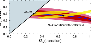
Figure 8: Projected likelihood contours are shown for Planck CMB and SNAP SN constraints on the $N=4$ gravitational transition model, including the contribution of scalar field potential energy prior to the transition. Models must lie below and to the right of the black line, outside the gray shaded region, with $\Omega_{m}({\rm today})\leq\Omega_{m}({\rm transition})$. The dark red contour shows the CMB 95$\%$ likelihood region, while the blue line indicates the family of geometric degeneracy models. The lighter red contour shows a weaker constraint from the CMB allowing for our uncertainty in the amount of spatial curvature. The black circles show the location of two specific models: a $\Lambda$CDM model, and an $N=4$ gravitational transition. The Hubble parameters for these two models have been chosen so that they have identical CMB anisotropy spectra. The yellow contours show the SN 95$\%$ likelihood regions for these two underlying models. Wherease both models are viable at present, they are clearly distinguishable with future observations.

To summarize, we have introduced a new scenario which generalizes the vacuum metamorpohsis model. In this scenario, gravitation undergoes a transition in which an order parameter built out of curvature tensors freezes at a constant value. After the transition, the matter content of the universe no longer determines the cosmological evolution — the expansion is ruled by the value of the order parameter. The onset of cosmic acceleration is sudden, and the effective dark energy equation-of-state is strongly negative, $w<-1$.

We have demonstrated that a range of these models satisfy a number of the standard tests of cosmology. There is excellent motivation to study these models further. The primary focus will be to analyze cosmological perturbations and the impact on structure formation. We can expect to find effects on the rate of growth of structure, the large-angle CMB anisotropy pattern, and weak gravitational lensing. The other focus will be to examine probes of the cosmic expansion suggesting the dark energy equation-of-state sharply Alam:2003fg ; Bassett:2002qu ; Corasaniti:2002bw ; Pogosian:2005ez dropped below $-1$ Kaplinghat:2003vf ; Huterer:2004ch ; Wang:2005ya , a distinct signature of this model.

- (1) A. D. Sakharov, Sov. Phys. Dokl. 12, 1040 (1968) [Dokl. Akad. Nauk Ser. Fiz. 177, 70 (1967 SOPUA,34,394.1991 GRGVA,32,365-367.2000)].
- (2) L. Parker and A. Raval, Phys. Rev. D 60, 063512 (1999) [Erratum-ibid. D 67, 029901 (2003)].
- (3) L. Parker and A. Raval, Phys. Rev. D 60, 123502 (1999) [Erratum-ibid. D 67, 029902 (2003)].
- (4) L. Parker and A. Raval, Phys. Rev. D 62, 083503 (2000) [Erratum-ibid. D 67, 029903 (2003)].
- (5) L. Parker and A. Raval, Phys. Rev. Lett. 86, 749 (2001).
- (6) L. Parker and D. A. T. Vanzella, Phys. Rev. D 69, 104009 (2004).
- (7) Y. Fujii and K.-I. Maeda, “The scalar-tensor theory of gravitation,” Cambridge University Press, 2003.
- (8) S. M. Carroll, V. Duvvuri, M. Trodden and M. S. Turner, Phys. Rev. D 70, 043528 (2004).
- (9) P. Teyssandier and Ph. Tourrenc, J. Math. Phys. 24, 2793 (1983).
- (10) D. Wands, Class. Quant. Grav. 11, 269 (1994).
- (11) V. Sahni and S. Habib, Phys. Rev. Lett. 81, 1766 (1998).
- (12) V. K. Onemli and R. P. Woodard, Phys. Rev. D 70, 107301 (2004).
- (13) I. I. Tkachev, Phys. Rev. D 45, 4367 (1992).
- (14) L. Parker, W. Komp, and D. A. T. Vanzella, Astrophys. J. 588, 663 (2003).
- (15) W. Komp, Ph.D. Thesis, University of Wisconsin, Milwaukee (2004).
- (16) R. R. Caldwell, M. Kamionkowski and N. N. Weinberg, Phys. Rev. Lett. 91, 071301 (2003).
- (17) A. G. Riess et al. [Supernova Search Team Collaboration], Astrophys. J. 607, 665 (2004).
- (18) R. A. Knop et al. [The Supernova Cosmology Project Collaboration], Astrophys. J. 598, 102 (2003).
- (19) D. N. Spergel et al. [WMAP Collaboration], Astrophys. J. Suppl. 148, 175 (2003).
- (20) W. L. Freedman et al., Astrophys. J. 553, 47 (2001).
- (21) W. J. Percival et al. [The 2dFGRS Collaboration], Mon. Not. Roy. Astron. Soc. 327, 1297 (2001).
- (22) A. C. Pope et al. [The SDSS Collaboration], Astrophys. J. 607, 655 (2004).
- (23) M. Zaldarriaga, D. N. Spergel and U. Seljak, Astrophys. J. 488, 1 (1997).
- (24) J. R. Bond, G. Efstathiou and M. Tegmark, Mon. Not. Roy. Astron. Soc. 291, L33 (1997).
- (25) G. Efstathiou and J. R. Bond, Mon. Not. Roy. Astron. Soc. 304, 75 (1999).
- (26) G. Huey, L. M. Wang, R. Dave, R. R. Caldwell and P. J. Steinhardt, Phys. Rev. D 59, 063005 (1999).
- (27) R. R. Caldwell and M. Doran, Phys. Rev. D 69, 103517 (2004).
- (28) U. Seljak and M. Zaldarriaga, Astrophys. J. 469, 437 (1996).
- (29) H. B. Sandvik, M. Tegmark, X. M. Wang and M. Zaldarriaga, Phys. Rev. D 69, 063005 (2004).
- (30) S. Burles, K. M. Nollett and M. S. Turner, Astrophys. J. 552, L1 (2001).
- (31) N. Deruelle and V. F. Mukhanov, Phys. Rev. D 52, 5549 (1995).
- (32) C. P. Ma and E. Bertschinger, Astrophys. J. 455, 7 (1995).
- (33) A. G. Kim, E. V. Linder, R. Miquel and N. Mostek, Mon. Not. Roy. Astron. Soc. 347, 909 (2004).
- (34) [SNAP Collaboration], arXiv:astro-ph/0405232.
- (35) see www.esa.int/science/planck
- (36) W. Hu, Phys. Rev. D 65, 023003 (2002).
- (37) W. Hu, arXiv:astro-ph/0407158.
- (38) D. J. Eisenstein, W. Hu and M. Tegmark, Astrophys. J. 518, 2 (1998).
- (39) U. Alam, V. Sahni, T. D. Saini and A. A. Starobinsky, Mon. Not. Roy. Astron. Soc. 354, 275 (2004).
- (40) B. A. Bassett, M. Kunz, J. Silk and C. Ungarelli, Mon. Not. Roy. Astron. Soc. 336, 1217 (2002).
- (41) P. S. Corasaniti, B. A. Bassett, C. Ungarelli and E. J. Copeland, Phys. Rev. Lett. 90, 091303 (2003).
- (42) L. Pogosian, P. S. Corasaniti, C. Stephan-Otto, R. Crittenden and R. Nichol, arXiv:astro-ph/0506396.
- (43) M. Kaplinghat and S. Bridle, arXiv:astro-ph/0312430.
- (44) D. Huterer and A. Cooray, Phys. Rev. D 71, 023506 (2005).
- (45) Y. Wang and M. Tegmark, Phys. Rev. D 71, 103513 (2005).