Smoothed Particle Inference:
A Kilo-Parametric Method for X-ray Galaxy Cluster Modeling

Abstract

We propose an ambitious new method that models the intracluster medium in clusters of galaxies as a set of X-ray emitting smoothed particles of plasma. Each smoothed particle is described by a handful of parameters including temperature, location, size, and elemental abundances. Hundreds to thousands of these particles are used to construct a model cluster of galaxies, with the appropriate complexity estimated from the data quality. This model is then compared iteratively with X-ray data in the form of adaptively binned photon lists via a two-sample likelihood statistic and iterated via Markov Chain Monte Carlo. The complex cluster model is propagated through the X-ray instrument response using direct sampling Monte Carlo methods. Using this approach the method can reproduce many of the features observed in the X-ray emission in a less assumption-dependent way than traditional analyses, and it allows for a more detailed characterization of the density, temperature, and metal abundance structure of clusters. Multi-instrument X-ray analyses and simultaneous X-ray, Sunyaev-Zeldovich (SZ), and lensing analyses are a straight-forward extension of this methodology. Significant challenges still exist in understanding the degeneracy in these models and the statistical noise induced by the complexity of the models.

1 Motivation

There are a large class of data analysis problems in astrophysics involving a model of a source that has a spectrum that varies spatially on the sky. In the case of the X-ray emission from clusters of galaxies, where the individual photon energies are recorded, the problem is especially prominent. In fact, much of the recent work in the X-ray analysis of clusters of galaxies has had the aim of obtaining a complete description of the density and temperature structure of the intracluster medium.

The X-ray emission from clusters of galaxies has been recently shown, using observations with the Chandra and XMM-Newton telescopes, to have a very complex distribution. In general, the surface brightness lacks circular symmetry. For example, cold fronts, or cluster gas that “sloshing” relative to the dark matter gravitational potential, is a significant perturbation from a spherically-symmetric gas distribution (Markevitch et al., 2000). “Radio bubbles”, which are displacements of cluster gas by relativistic radio-emitting plasma, have complex morphologies and vary from cluster to cluster. Sanders et al. (2004) have identified a “swirl” in the temperature structure of the Perseus cluster possibly due to rotation of the cluster gas. There may also be ripples or waves in the cluster gas (Fabian et al., 2003). Neither are clusters isothermal: Kaastra et al. (2003) and Buote et al. (2003) have questioned the assumption that the cluster gas can even approximately be described by a single phase as a function of radius. In fact, they find evidence that the temperature can vary at a single radius by a larger factor than the average temperature drops radially across the entire cluster.

Recently, the gross spectrum from clusters of galaxies was shown to be inconsistent with simple models of cooling flows (e.g.  Peterson et al., 2001). The confusion over what this result means clearly precludes the use of any simple theoretical template in the construction of a model of the intracluster medium. Our goal in this paper is therefore to provide a flexible method that is capable of reproducing all of the complexities we have mentioned above. This method must necessarily utilize both the spectral and spatial information in a dataset and should still be effective with datasets that have relatively low numbers of X-ray counts.

In the literature is a large number of diverse techniques for analyzing X-ray data from galaxy clusters. The methods range from fitting isothermal spectra to square grids of photons across the detector plane (e.g.  Markevitch et al., 2000) to imaging deprojection techniques through “onion-peeling” methods (e.g.  Fabian, Cowie & Grindlay, 1981). Fitting adaptively-binned data to isothermal models has also proved useful (Sanders et al., 2004) and the onion-peeling technique has been extended to spectroscopic deprojection (Arabadjis, Bautz & Garmire, 2002; Arnaud, 2001; Kaastra et al., 2003; Andersson & Madejski, 2004). Other methods include image smoothing, gross spectral fitting, and inversion of spectral hardness ratios (Sanderson et al., 2004).

We break with these previous methods in two important ways. First, we use the spectrum and image of a source on an equal footing. Traditional analyses extract a spectrum from a piece of the detector plane and then use the integrated number of photons as a proxy for the true source image. However, this process is only approximately correct in the presence of broad point-spread functions that are energy-dependent. Even the concept that there is an “image” and a “spectrum” for a spatially-resolved source is misleading, since in reality there is a spatially-varying emissivity at a given energy. We propose to use a Monte Carlo calculation to forward-fold a complex model to predict detector positions and CCD energies for each photon. Secondly, we construct a model that is flexible enough to allow for extremely complex gas temperature and density distributions in clusters. For example, a common approach is to assume a single temperature for a given set of photons and fit for its value. In contrast, our procedure is to allow for a multi-temperature distribution, and then allow the method to sharpen the temperature distribution if it is close to a single temperature. This approach is motivated by the observations outlined in the first paragraph that clusters are complex. We achieve this complexity by modeling the emissivity from clusters as using conglomerations of emissivity particles, smoothed for ease of interpretation.

The construction of underlying model distributions from linear combinations of simple basis functions is well-founded in modern Bayesian image processing: indeed, the “massive inference” method of Skilling (1998) has been found to be a powerful technique for the reconstruction of one dimensional spectra and two dimensional images. This work may be seen as a practical application of the basic premises of massive inference to the problem of astronomical X-ray data analysis, with some of the refinements compromised in the name of pragmatism. Skilling et al. coined the term “atom” for the indivisible unit of image flux; to avoid confusion with the atomic physics terminology of X-ray spectroscopy we translate atom into particle and draw an analogy with numerical simulations of galaxy clusters. Where in the first instance our goal is to model X-ray data, it will become clear that this “smoothed particle inference” (SPI) methodology offers great opportunities for further analysis and physical interpretation. This work also borrows heavily from some independent pioneering work by Jernigan & Vezie (1996). There a Monte Carlo approach was used to invert X-ray data by interating a non-parametric model, while matching the simulation with the X-ray events.

In this paper, we describe the SPI method in considerable detail, highlighting the two novel aspects introduced above. We then apply the method on realistic simulated datasets for both EPIC and RGS, and show that it works. We then demonstrate some of the benefits of the methodology with regard to extracting and displaying the information in the data.

In two companion papers, we apply the method to XMM-Newton Reflection Grating Spectrometer (RGS) observations of the Perseus and Virgo clusters (Peterson et al., 2006) and XMM-Newton European Photon Imaging Camera (EPIC) observations of Abell 1689 and RXJ0658-55 (Andersson et al., 2006).

2 Methodology

This section is organized as follows. We first describe our choice of model, a set of spatially Gaussian X-ray plasma emitters of an assigned spectral type. Then, we discuss X-ray Monte Carlo techniques to propagate this model through the instrument response. We discuss the ensuing two-sample likelihood statistic used to assess the statistical significance of the model. Finally, we describe the use of Markov Chain techniques to iterate the model and explore the parameter space.

2.1 Smoothed Particles in a Luminosity Basis

We have argued in the previous section that a “non-parametric” method, or rather, a method with thousands of parameters, is required to describe the current X-ray data. In particular, a more unified modeling approach, embracing all the complex aspects of clusters that have recently been discovered (cold fronts, temperature radial gradients, local non-isothermality, lack of circular symmetry in the temperature distribution) is now required.

Consider a “blob”, or “smoothed particle”, of plasma, described by a spatial position, a Gaussian width, a single temperature, a set of elemental abundances, and an overall luminosity. A model of a cluster of galaxies may be constructed from a set of such particles. There are a number of advantages to doing this. The model has enough freedom to reproduce all of the salient features of cluster gas distributions, and can form complex density and temperature structures. Particles with different temperatures can occupy the same position and therefore multi-phase temperature distributions can be constructed. There is also no global spherical symmetry that is imposed on the particle configuration, although they are themselves spherically symmetric. Another powerful aspect of using smoothed particles is that they can be mapped from one space to another in a straightforward way: for example a collection of smoothed particles representing X-ray luminosity may be manipulated in order to derive the corresponding SZ decrement map. This approach is somewhat similar to the methods used in smoothed particle hydrodynamics (SPH), except here the method decide the properties of the smoothed particle, rather than a set of hydrodynamical equations. For this reason, we refer to the method as “smoothed particle inference”.

Assuming an X-ray source is optically-thin, we can write the differential luminosity per volume due to a set of smoothed Gaussian particles as

$$\frac{d^{2}L}{dVdT}=\sum_{i}L_{i}\delta\left(T-T_{i}\right)\frac{e^{-\frac{\left|{{\bf x}-{\bf x_{i}}}\right|^{2}}{2{\left(D_{A}\sigma_{i}\right)}^{2}}}}{\left(2\pi{\left(D_{A}\sigma_{i}\right)}^{2}\right)^{3/2}}$$ (1)

where $L_{i}$ is the luminosity per particle in ergs per second, $T_{i}$ is the temperature of the $i$th particle in keV, $D_{A}$ is the angular diameter distance in cm, $\sigma_{i}$ is the angular size in radians, ${\bf x_{i}}$ is the location of the particle in three dimensions expressed in cm. We achieve the differential luminosity per solid angle by integrating along the line of sight, $dz$,

$$\frac{d^{2}L}{d\Omega dT}=D_{A}^{2}\int_{-\infty}^{\infty}\frac{d^{2}L}{dVdT}dz.$$ (2)

This can be rewritten as

$$\frac{d^{2}L}{d\Omega dT}=\sum_{i}L_{i}\delta\left(T-T_{i}\right)\frac{e^{-\frac{\left|{{\bf x}-{\bf x_{i}}}\right|^{2}}{2{\left(D_{A}\sigma_{i}\right)}^{2}}}}{\left(2\pi{\left(D_{A}\sigma_{i}\right)}^{2}\right)}$$ (3)

where ${\bf x_{i}}$ is now the two dimensional spatial position of each smoothed particle. The differential flux per unit solid angle per unit energy, $\frac{d^{2}F}{dEd\Omega}$, in units of photons per second per $\mbox{cm}^{2}$ which is the actual observable, is then obtained by first calculating the differential flux per unit energy, $\frac{dF}{dE}$,

$$\frac{dF}{dE} = \frac{1}{4\pi D_{L}^{2}}\int_{0}^{\infty}dT\frac{d\alpha}{dE}\frac{dEM}{dT}$$

$$= \frac{1}{4\pi D_{L}^{2}}\int_{0}^{\infty}dT\frac{d\alpha}{dE}\frac{dL}{dT}\frac{1}{\Lambda}$$

where $D_{L}$ is the luminosity distance in cm, $\Lambda$ is the cooling function in units of $\mbox{ergs}\mbox{cm}^{3}s^{-1}$, $\frac{dEM}{dT}$ is the differential emission measure, and $\frac{d\alpha}{dE}$ is the line (or continuum power) which is predicted uniquely given a set of elemental abundances and a temperature in units of $cm^{3}s^{-1}keV^{-1}$. Note that the cooling function is the energy averaged integral of $\frac{d\alpha}{dE}$. The differential flux per solid angle per energy is then obtained by combining equation 3 and equation 4,

$$\frac{d^{2}F({\bf\theta},E)}{dEd\Omega}=\sum_{i}\frac{L_{i}}{4\pi D_{L}^{2}\Lambda(T_{i},\{A_{i}\})}\times$$

$$\frac{d\alpha}{dE}(E|T_{i},z_{i},\{A_{i}\})~{}\frac{e^{-\frac{\left({{\bf\theta}-{\bf\theta_{i}}}\right)^{2}}{2\sigma^{2}}}}{\left(2\pi\sigma^{2}\right)}.$$ (5)

where ${\bf\theta}$ are angular coordinates on the sky, $\sigma$ is now in angular units, $D_{L}$ is the luminosity distance in cm, $\Lambda(T_{i},\{A_{i}\})$ is the temperature and metallicity-dependent cooling function, and $\frac{d\alpha}{dE}$ is the energy-dependent line (or continuum) power function, which describes the probability of a photon having a given energy $E$ as a function of temperature.

We have purposely chosen to use luminosity as the basis for our smoothed particles, rather than, say, gas density. If we had parameterized in terms of the gas density then predicting the luminosity would require, essentially, a summation over all particles to reconstruct the density field and then the squaring of the result. In this case, the complete luminosity field would have to be reconstructed following the alteration of a single particle. Later, we will demonstrate that using a luminosity basis will simplify the calculation considerably but not quantitatively change the results. We are also anticipating that in using this method in combination with SZ observations, it will still be preferable to use the luminosity as the basis rather than a Compton-y parameter basis since the calculation of the X-ray instrument response is likely to be much more involved.

2.2 X-ray Monte Carlo Methods

We convert the luminosity at each energy and spatial position into a quantitative prediction for probability of the numbers of photons at a given detector position and energy via a Monte Carlo calculation. More explicitly, our goal is the calculation of the probability of detection, $D$, given the instrument response function, $R$, and the photon source model, $S$. This is expressed as,

$$D({\bf u},p)=\int dE~{}d\Omega~{}R({\bf u},p~{}|~{}E,{\bf\Omega})~{}\frac{d^{2}F}{dEd\Omega}(E,{\bf\Omega})$$ (6)

where ${\bf u}$ are the detector position vector, $p$ is the measured detector energy, $\Omega$ is the sky position vector, and $E$ is the intrinsic energy of the photon. This is a three-dimensional integral: it is most efficiently calculated using a Monte Carlo approach. In Peterson, Jernigan, & Kahn (2004), we describe the calculation of this integral for the Reflection Grating Spectrometers (RGS) on XMM-Newton. We have also written a companion Monte Carlo for the European Photon Imaging Cameras (EPIC) on XMM-Newton (Andersson et al., 2006). We do not describe these calculations in detail here, but instead briefly outline their use in the context of smoothed particle simulation.

In the Monte Carlo calculation, photons are simulated sequentially via conditional probability functions. Mirror, grating, and detector responses are included in the calculation. For the RGS simulation, photons are manipulated using a set of dispersion and cross-dispersion response functions, CCD pulse-height redistribution functions, and exposure maps. For the EPIC Monte Carlo, photons are constructed using the point-spread function, vignetting, CCD pulse-height redistribution functions, and the exposure map. In general, the functions are both energy and off-axis angle dependent and the calculation of these functions involves a sequence of convolutions. The response functions are calculated on coarse grids, and then interpolated using a Monte Carlo method (Peterson, Jernigan, & Kahn, 2004). Photons are removed in proportion to the relative response probability, in order to properly calculate the effective area, which is also off-axis angle and energy dependent.

For the purpose of simulating the X-ray emission from a set of SPI particles, a set of simulated photons is assigned to a particular particle. The particle parameters are the temperature ($T$), set of abundances, position ($\phi$, $\psi$), Gaussian width ($\sigma$), and possibly the redshift. For each photon, the wavelength is first chosen from the probability distribution described by the emissivity function corresponding to the temperature and set of elemental abundances of that particle. Its position is then perturbed from the nominal center of that particle ($\phi$, $\psi$) by a random Gaussian step having width equal to $\sigma$.

The photon flux per particle, $F_{i}$, is calculated by computing,

$$F_{i}=\frac{N}{A_{\rm eff}\tau}$$ (7)

where $A_{\rm eff}$ is the peak effective area in units of $\mbox{cm}^{2}$, $\tau$ is the exposure time in units of $s$, and $N$ is the number of photons simulated before removing any photons in the Monte Carlo calculation. The luminosity, $L_{i}$ per particle can be calculated by computing,

$$L_{i}=F_{i}\frac{\Lambda_{i}}{P}4\pi D_{L}^{2}$$ (8)

where

$$P=\int dE\frac{d\epsilon}{dE}$$ (9)

and $\frac{d\epsilon}{dE}$ is the emissivity per energy interval in units of $\mbox{cm}^{2}\mbox{s}^{-1}\mbox{ergs}^{-1}$.

2.3 The Likelihood Function

We quantify the goodness of fit of a given set of SPI particles via the likelihood function of their parameters. In general, the likelihood is a function dependent on both predicted and actual data, whose form embodies the analyst’s understanding of the measurement errors, and is understood as the probability of getting the data given the parameters of the model. Ordinarily, the predicted data are calculated to arbitrary precision within the context of the model under investigation: this is not the case here. The Monte Carlo simulation procedure outlined above, while needed to deal correctly with the energy-dependent and spatially varying telescope response, provides predicted data that are themselves uncertain, being the outcome of a Poisson process. We can view the output of the telescope, and the output of the simulation, as two independent data streams emanating from the same underlying physical process (emission from the cluster followed by detection at the telescope). The likelihood function then quantifies the misfit between the two datasets.

Note that given infinite simulation time, predicted data can be computed with infinite precision within the context of the limitations of the instrument model; clearly any likelihood statistic used should revert to the more familiar form in this limit. Moreover, we note that all likelihood functions are necessarily approximations to an unknown function (that indeed, should itself form part of the data model). We should be satisfied with a likelihood that captures the essence of the misfit, and satisfies any limits such as that above. Statistics for the two Poisson sample situation have not been well-developed in the statistical literature; possibly it has been deemed preferable to find alternative ways of computing predicted data exactly rather than press on with effectively two sources of measurement error. Where attempts have been made, they have made use of Gaussian approximations valid only in the limit of large numbers. In the appendix we give a discussion of a number of routes to a likelihood function applicable to the low counting statistics of X-ray datasets, and show how they recover the correct form in the limit of infinite simulation time. We give below the form of the likelihood $L_{2}$ that we use in practice, and note that in its normalized form ($L_{2N}$) that $-2\log L_{2N}$ is distributed as $\chi^{2}$ with the number of degrees of freedom equal to the number of bins. while not required by the analysis, we find that this provides a valuable check on the pure goodness of fit of the models, giving confidence in the results.

In general, we find that the results are relatively insensitive to the exact choice of likelihood statistic and the differences are largest when the data is extremely sparse and there are few photons: in subsection 2.3.2 below we outline our approach for avoiding this eventuality. We experimented with the likelihood functions in the next section and found the reconstruction to produce similar results.

2.3.1 Two Sample Likelihood Statistic

The basic datum is a number of photons in a three dimensional bin $(u_{1},u_{2},p)$. The bin size may be set by physical limits such as the extent of the CCD pixel, or be imposed given some understanding of, for example, the spectral resolution of the instrument. The simulated photons are then binned on the same grid. Assume that we have $n$ photons in the observed dataset, and have simulated $m$ photons from our model: in the $i^{\rm th}$ bin we have $E_{i}$ simulated photons, and $O_{i}$ observed photons. Since the photons falling into a set of bins will follow a multinomial distribution, we obtain for the data photons the likelihood function

$$L_{O}=n!\prod_{i}\frac{{\left(\lambda_{i}\right)}^{O_{i}}}{O_{i}!}$$ (10)

where $\lambda_{i}$ is the probability of getting a photon in that bin. The multinomial distribution is the Poisson distribution but with total number of photons fixed. Treating the simulated photons in the same way, we get

$$L_{s}=m!\prod_{i}\frac{{{\left(\lambda_{i}\right)}}^{E_{i}}}{E_{i}!}$$ (11)

In doing so we have suggested that the simulated photons be considered to be from a separate, independent, experiment with its own likelihood. The joint likelihood is then just the product of the two experiments’ likelihoods. In the appendix we discuss two routes to dealing with the value of the parameters $\lambda_{i}$: one can see that a reasonable guess is to estimate $\lambda_{i}$ from the data and set $\lambda_{i}=(O_{i}+E_{i})/(m+n)$:

$$L_{2}=n!m!\prod_{i}\frac{{{\left(\frac{O_{i}+E_{i}}{m+n}\right)}}^{O_{i}}{{\left(\frac{O_{i}+E_{i}}{m+n}\right)}}^{E_{i}}}{O_{i}!E_{i}!}$$ (12)

We use this form when comparing exploring the parameter space as outlined in the next section. It is possible to re-normalize these likelihood functions, such that they will approximately follow the $\chi^{2}$ distribution (Cowan, 1998). This is done by dividing by the same expression with the probability estimates replaced by the actual number of counts. The result for the likelihood given above is written as

$$L_{2N}=\prod_{i}\frac{\frac{{{\left(\frac{O_{i}+E_{i}}{m+n}\right)}}^{O_{i}}{{\left(\frac{O_{i}+E_{i}}{m+n}\right)}}^{E_{i}}}{O_{i}!E_{i}!}}{\frac{{{\left(\frac{O_{i}}{n}\right)}}^{O_{i}}{{\left(\frac{E_{i}}{m}\right)}}^{E_{i}}}{O_{i}!E_{i}!}}=\prod_{i}\frac{{{\left(\frac{O_{i}+E_{i}}{m+n}\right)}}^{O_{i}+E_{i}}}{{{\left(\frac{O_{i}}{n}\right)}}^{O_{i}}{{\left(\frac{E_{i}}{m}\right)}}^{E_{i}}}$$ (13)

By construction, $-2\log{L_{2N}}$ is approximately distributed as $\chi^{2}$ with the number of degrees of freedom equal to the number of bins. We use $L_{2N}$ for checking that a reasonable fit is being obtained by the method (see also section 2.4.5), which will be near the number of degrees of freedom for a good fit. In the appendix we demonstrate how this statistic approaches the two sample $\chi^{2}$ statistic that we used in the large $m$ and $n$ limit. $L_{2}$ is used for the parameter iteration, since it analgous to the one-sample likelihood.

2.3.2 Three-Dimensional Adaptive Binning

The statistics that we have discussed in the previous section require the events to be binned on a arbitrary three-dimensional grid. For a non-dispersive spectrometer, the natural minimal grid for this would be to design bins to reasonably sample the point-spread function for the two spatial dimensions and the energy resolution kernel for the spectral dimension. For a dispersive spectrometer, the angular dispersion resolution kernel would define the bins in the dispersion direction. In either case, however, it is found that, for virtually all observations of clusters of galaxies, the numbers of minimal bins are very large indeed, and that the photons fill the three dimensional grids extremely sparsely. In fact, most bins typically contain either 0 or 1 photons. Simple grouping of these minimal bins will result in severe loss of spectral and/or spatial resolution. Therefore, a more efficient binning approach deserves some consideration. Although the statistics discussed in the previous section are capable of handling low numbers of photon counts, we are pushed toward fuller bins to reduce computation time. Additionally, we show below that the fluctuation induced on the statistic by the Monte Carlo calculation depends on the number of bins, such that a smaller number of bins is preferred.

For these reasons, we have developed an algorithm to adaptively bin the data in the three dimensions similar to other adaptive binning methods. To do this, we first consider the entire three-dimensional data space. We create the binning grid by bisecting the data space in one dimension at a time. The dimension to bisect is chosen from the relative length of the bin in each dimension. The longer dimension is always bisected. If the relative sizes are the same the dimension is selected randomly. Each bin is bisected for as long as any bin has more than $N$ counts; most of the bins will contain on average $N/2$ photon counts by the time the binning has been completed. Typically, $N$ is chosen to be 10 or 20, but this varies between applications. For instance in a dataset with extremely low flux the bins can be made with fewer photons. There is also the possibility of weighting the bin size in any dimension with some factor $n$. For example, if spectral accuracy is preferred over spatial accuracy the bins in the spectral dimension can be chosen to be on average $n$ times smaller than the spatial bins. After the bins have been determined for the data photons, they remain fixed. We then use a binary tree algorithm to rapidly place new simulated photons into the appropriate bin. The two-sample statistic given in the previous section can then be calculated as a product over all the bins.

2.4 Parameter Iteration

After model generation and likelihood calculation, the third major component of the method is the sequence of model parameter iteration. We have found several complications to the usual methods of parameter iteration that are particularly problematic with the high-dimensional parameter model that we are considering in this paper. In the following subsections we discuss several aspects of this part of the analysis chain.

2.4.1 Markov Chain Monte Carlo Exploration

We explore the parameter space of the smoothed particle model with the Markov Chain Monte Carlo (MCMC) method, the use of which has recently become widespread in the field of Bayesian data analysis (see Gilks, Richardson & Spiegelhalter, 2003, for an excellent introduction). MCMC is a technique for sampling the probability distribution of a model’s parameters; in this case, the dimensionality of the parameter space is extremely high, prohibiting brute force grid calculations and condemning gradient-based optimization to failure by being trapped in local likelihood maxima. MCMC is a very efficient and powerful way of exploring such high-dimensional spaces, returning a list of sample cluster models all of whom are consistent with the data, and whose number density in parameter space follows the probability density.

Possession of the entire parameter probability distribution, in the form of a list of samples, opens up possibilities not available to other methods. The distributions of particle parameters, for example, can be used to estimate the average distributions of cluster quantities (such as temperatures and densities). These averages come with well-defined uncertainties trivially derived from the samples: one may probe the range of distributions that are consistent with the data. MCMC is now the standard tool for cosmological data analysis (see e.g.  Lewis & Bridle, 2002; Tegmark et al., 2004). MCMC has been applied to simple cluster modeling using SZ and lensing data (Marshall et al., 2003), and X-ray and SZ data (Bonamente et al., 2004). To date, the use of MCMC in astrophysics has been restricted to relatively modest numbers of parameters. However, it is when using large numbers of parameters to model complex datasets that the full power of the technique is realised.

As usual, the target probability distribution is the posterior density $P$, given by Bayes’ theorem as

$$P(\{\theta\}|D)\propto L(D|\{\theta\})\pi(\{\theta\}).$$ (14)

Here, $L$ is the likelihood function introduced above, with the notation emphasizing its dependence on the observed data $D$ given the parameter set $\{\theta\}$. $\pi$ is the prior probability distribution of the model parameters: in this work we use uninformative priors on all parameters, restricting ourselves to uniform distributions over broad finite ranges.

We give here the briefest of introductions to the Metropolis-Hastings algorithm (Metropolis et al., 1953; Hastings, 1970) that we use to sample the posterior density, and then provide details of the implementation in the following subsections. Following the evaluation of the likelihood associated with an initial point in parameter space, $P_{1}\equiv\left(\theta_{1},\theta_{2},\ldots,\theta_{n}\right)$, a new point, $P_{2}$ is drawn from a proposal distribution. This proposal distribution is required to be symmetric about the current position to ensure successful sampling of the target distribution. If the likelihood of the new point is higher than the likelihood of $P_{1}$ then the new point is accepted. Otherwise, the point is accepted only if a uniform random number between 0 and 1 is less than the ratio of likelihoods, $\frac{L(P_{1})}{L(P_{2})}$. This is known as the Metropolis-Hastings acceptance criterion. If the new point is not accepted, then the old point is repeated in the chain of parameters. While this basic algorithm is very simple, the efficiency of the exploration of the parameter space depends strongly on the form of the proposal distribution, which we discuss in the following two subsections.

2.4.2 Adaptive Proposal Distribution

As we mentioned in the previous section, the method of picking the next point in the Markov chain can either be by taking a step from some fixed distribution or it can be modified dynamically. In dealing with the large number of parameters in the smoothed particle fits, we have found that an adaptive proposal distribution is necessary. Initially, the proposal distribution is chosen to be a Gaussian of fixed width, $\sigma$. After the Markov chain has taken a few steps, we calculate the standard deviation, $\sigma^{\prime}$, of the new estimate of the target posterior distribution. We then use $\sigma^{\prime}$ as an estimate for the new step in the proposal distribution. Large excursions in parameter space, however, can sometimes bias this standard deviation estimation. Therefore, we have constructed a different standard deviation estimator with some built-in “memory loss”, such that earlier steps are weighted less strongly. The proposal step width, $\sigma^{\prime\prime}$ is calculated according to

$$\sigma^{\prime\prime}=\left(\frac{\sum_{i}(1+\epsilon)^{i}p_{i}^{2}}{\sum_{i}(1+\epsilon)^{i}}-\frac{\left(\sum_{i}(1+\epsilon)^{i}p_{i}\right)^{2}}{\left(\sum_{i}(1+\epsilon)^{i}\right)^{2}}\right)^{\frac{1}{2}}$$ (15)

where $p_{i}$ is the parameter value at the $i^{\rm th}$ iteration and the sum is over all the iterations. $\epsilon$ is a constant taken to be $0.01$ that causes the earlier iterations to be de-weighted. If $\epsilon$ were zero, the formula would result to the normal standard deviation formula; an infinite value for epsilon implies the normal non-adaptive Gaussian proposal distribution. With finite $\epsilon$, the individual steps no longer exactly satisfy detailed balance, as the proposal distribution is slightly different between the current and trial sample positions. If epsilon is set sufficiently small (although not so small as to restrict the movement of the chain) then a large number of past sample positions are used to determine the proposal distribution widths, and consequently the differences between any successive proposal distributions are very small. The parameter update method then asymptotically becomes a true Markov chain. In practice these differences are completely negligible compared to the large deviations from unity of the likelihood ratios. Quantitatively, we found that this holds whenever $2\Delta\log{L}\gg\frac{\Delta\sigma^{\prime\prime}}{\sigma^{\prime\prime}}\approx\epsilon$. In practice $2\Delta\log{L}$ is much larger than one and we take $\epsilon$ to be 0.01.

The proposal step is then taken to be $2.38\sigma^{\prime\prime}d^{-\frac{1}{2}}$, where $d$ is the number of dimensions. This is the optimal step size for uncorrelated Gaussian distributions, such that the acceptance rate times the RMS step size is maximized for this value. In the large $d$ limit, a rejection rate around 77$\%$ is expected (Roberts, Gelman, & Gilks, 1997). A successful chain will, after the burn-in period, explore the posterior distribution with this rejection rate, and the proposal distribution in any given parameter direction will asymptote to the Gaussian approximation to the marginalized posterior.

2.4.3 Global and local parameters iteration sequence

In a typical SPI emission model there are two kinds of parameters. The first kind are local parameters, describing the individual properties of the particles. These are the temperature, position, size, and elemental abundances for each particle. The second kind are global parameters for describing properties of the entire data set. These parameters are the background parameters and the absorption column density. The order in which these parameters are varied was found to have a strong influence on the speed of the chain convergence: the variation sequence has been under considerable study in the development of this method.

Firstly, it was found that the local parameters for a particular particle should be varied separately while holding the parameters of the other particles fixed and the global parameters fixed. We believe that this is a valid technique since any particle can be interchanged with any other particle and therefore we can exploit this symmetry by not considering the full degeneracy of all of the particles parameters. We do, however, vary the set of particle parameters – position, temperature, elemental abundances, and Gaussian size– simultaneously since these parameters may be highly correlated. Varying each set of particle parameters separately speeds up the calculation by several orders of magnitude, as only the photons associated with that particle need to be resimulated.

Secondly, we found that after changing the global parameters the particle parameters needed to be varied for at least one iteration in order for the system to re-equilibrate and remain in the desired high probability region. This is necessary since there may be some correlations between the positions of the particles, for example, and global background parameters. Therefore, the particle parameters must be allowed to move somewhat before rejecting a new set of global parameters. Without this consideration, we found some global parameters became pinned to sub-optimal values.

Thirdly, we found it necessary to regenerate a completely new set of photons for a particular set of parameters frequently. This is necessary due to the Monte Carlo nature of the calculation: there is statistical noise in the likelihood value itself. Although we believe the two sample likelihood properly deals with this statistical noise in modifying the likelihood surface, it does not deal with the parameters drifting to a particular non-optimal value only because it received a favorable set of photons. Frequent regeneration of the photons simply cancels this effect and restores the mobility of the Markov chain.

These three considerations lead us to the following sequence of parameter iteration. Consider that we have $n$ particles with local parameters, $l^{i}_{j}$, for the $i$th particle and the $j$th particle parameter. Assume also that we have a set of global parameters $g_{k}$ for the $k$th parameter. The following sequence of parameter variation is then used for each iteration:

1. Vary values of $l^{i}_{j}$ to new values $l^{\prime i}_{j}$, holding the parameters of all other particles fixed, and compute the likelihood. Take the new values if the statistic conforms to the acceptance criterion. Repeat this step for each of the particles.

2. Regenerate all photons for $g_{k},l^{\prime i}_{j}$ and compute the likelihood.

3. Vary the values of $g_{k}$ to a new point $g_{k}^{\prime}$. Hold the values of $l^{i}_{j}$ fixed at the previous values.

4. Vary the values of $l^{i}_{j}$ to new values $l^{\prime\prime i}_{j}$, holding the parameters of all other particles fixed, and compute the likelihood. Take the new values, if the statistic conforms to the acceptance criterion. Repeat this step for each of the particles.

5. Regenerate all of the photons $g_{k}^{\prime}$ and possibly the new values of $l^{i}_{j}$. Compare the value of the likelihood at this point with that obtained in the second step. Take the new value of $g^{\prime}_{k}$ and values of $l^{\prime\prime i}_{j}$, if it conforms to the acceptance criterion. Otherwise, return to the previous values of both $g_{k}$ and $l^{\prime i}_{j}$ at the second step.

The absence of a Metropolis comparison in step 3 indicates a departure from the standard Markov chain: in fact, this step can be thought of as the splitting off of a new chain which explores the posterior conditional on the value of $g_{k}^{\prime}$. After some exploration of the local parameter space, this chain is then compared with its parent (left behind at the known sample position $g_{k}$) and the fittest (in the Metroplis-Hasting sense) survives in step 4. Strictly speaking this process does not conserve detailed balance: however, we have checked that the departure of this algorithm from the proper format does not affect the convergence on the target posterior distribution, at least in simple cases as we demonstrate in Appendix 2.

2.4.4 Increase of the Over-simulate factor and Statistical Noise

Since we have used a Monte Carlo calculation to calculate the likelihood statistic for the highly-complex smoothed-particle model, there is unavoidable statistical noise in the likelihood function. The same set of parameters will produce a slightly different value of the likelihood statistic every time they are simulated. This Monte Carlo noise can be reduced by increasing the “over-simulate factor,” the ratio of the simulated photons compared to the number of photons in the data set. In practice, a value of the over-simulate factor of 10 or so can be easily accommodated, but much larger values become tedious when working on a single workstation. The statistical fluctuation in the two sample normalized statistic scales empirically as

$$\sigma_{L_{2N}}\sim\sqrt{\frac{\mbox{number~{}of~{}bins}}{\mbox{over-simulate~{}factor}}}$$ (16)

such that the fluctuation can be reduced by both increasing the simulation factor and reducing the number of bins. Normally, this ratio is significantly larger than one, and therefore this is likely to significantly broaden the posterior distribution of any parameters. However, this merely makes the method conservative: the posterior distributions we derive contain the smaller true distribution. This is illustrated in Figure 6.

2.4.5 Particle Number and the Evidence

Initially, we experimented with methods that may change the number of particles dynamically, during the evolution of the Markov chain. However, we found that any advantage that this method may have had, in reducing the number of smoothed particles and their associated parameters, was outweighed by the complications added to the fitting procedure. In particular, it was difficult to determine what to do with the parameters of the particles that were newly created or recently destroyed when the particle number changed. The use of adaptive steps within this scheme was also problematic. Therefore, we fix the number of particles and do not vary this during the parameter iteration, instead opting for a more approximate approach to determining a suitable number of particles.

We calculate (albeit approximately) the “evidence” of the smoothed particle model as a function of particle number. The evidence is the integral of the likelihood function $L$ times the prior distribution, $f(p_{i})$ over all parameters($p_{i}$):

$$E=\int\prod_{i}dp_{i}Lf(p_{i})$$ (17)

The evidence works by penalizing overly complex models (such as those with too many particles) wwith a lower evidence (see e.g.  McKay, 2003; Ó’Ruanaidh & Fitzgerald, 1996; Marshall et al., 2003, for introductions to the use of the evidence). We estimate the evidence by the method of thermodynamic integration (Ó’Ruanaidh & Fitzgerald, 1996), raising the likelihood to some power during the initial stages of the MCMC process and increasing this power steadily from 0 to 1. In our studies, the evidence increased dramatically with increasing particle number for less than $\sim 100$ smoothed particles but was then relatively flat for larger particle numbers. This number of course varies from dataset to dataset: we use the smallest number of particles possible (indicated by the turnover in evidence, where the improvement in goodness-of-fit starts to become insignificant) in the interests of both the economy of hypotheses and also of saving computation time.

The method requires one to choose both the over-simulate factor and the number of smoothed particles. The former is chosen to be as large as possible without the method taking too long, and the latter is chosen to be as large as possible given the criteria of the previous paragraph. Having finite values for the over-simulate factor limits the precision of the method, but this was found to be unimportant for many applications. Limiting the number of particles via consideration of the evidence prevents fitting of the noise with an overly complex model.

3 Model Interpretation Methods

There is an impressive variety of techniques that can be applied to the results of the smoothed particle inference. The output of the MCMC process consists of a set of parameters, both global and local, for the given number of smoothed particles, for each iteration. Thus, the usual marginalized posterior probability distributions can be generated by histogramming the history of parameter values (see Fig. 4). The interpretation of the smoothed particle parameters is not always straightforward, but a wealth of information resides in the MCMC samples. SPI is essentially a method for translating noisy X-ray data into uncertain emission components: the Markov chain process retains the correlations between components such that the manipulation of the samples can reveal much about the gross and detailed properties of the emitter. We discuss just some of the possible inference techniques below. As always, caution has to be used in only using samples taken after the chain has reached the stationary distribution.

To demonstrate these inference techniques we have simulated a cluster model with two spatially separated isothermal components to which we apply our method. This choice of simplistic simulation reflects both our desire to demonstrate the algorithm on a relatively easily-interpreted problem, but also the difficulty of generating realistically complex mock datasets. To make a simple demonstration of the features of the method we have chosen to simulate a double cluster with two isothermal components. This will test the ability of the method to estimate single temperatures as well as to separate different components in a dataset, both spatially and spectrally. The method is applied to real datasets in two companion papers, Peterson et al. (2006) and Andersson et al. (2006).

In this work we perform separate inferences for the XMM-Newton EPIC and XMM-Newton RGS detectors. In the EPIC run we expect to be able to resolve the spatial structure of the clusters in detail due to the high spatial resolution (PSF FWHM $\sim 6^{\prime\prime}$) of the instrument datasets. For the RGS run the spatial resolution will be low in the dispersion direction of the spectrometer; however we expect to resolve spectral features in finer detail.

3.1 A simulated double-cluster model

The spatial model of the simulated cluster consists of two beta-models,

$$S(r)=S_{0}\left(1+\left(\frac{r}{r_{c}}\right)^{2}\right)^{-3\beta+0.5}$$ (18)

where $S(r)$ is the source surface brightness at angular radius $r$ and $r_{c}$ is the angular core radius. The beta models are separated diagonally by $1^{\prime}$. Each of the two clusters is modeled spectrally with a MEKAL (Mewe, Gronenschild, & van den Oord, 1985; Mewe, Lemen, & van den Oord, 1986; Kaastra, 1992; Liedahl, Osterheld, & Goldstein, 1995) model for the thermal plasma with Wisconsin (Morrison & McCammon, 1983) photo-electric absorption for the Galactic column. The cluster plasma temperatures were chosen separately for the EPIC and RGS simulations due to the different energy sensitivity of the two instruments. In the RGS run the two beta models have isothermal temperatures of kT = 1 keV  and kT = 3 keV  respectively whereas in the EPIC run these temperatures are at kT = 3 keV  and kT = 6 keV .

Metal abundances are set at 0.5 Solar, the redshift is fixed at $z=0.2$ and both clusters are absorbed by a corresponding Hydrogen column of $4\times 10^{20}~{}\mathrm{cm^{-2}}$. The beta model parameters for the clusters were set to $\beta=0.7$, $r_{c}=40^{\prime\prime}$ and $\beta=0.5$, $r_{c}=15^{\prime\prime}$ for the lower left and the upper right cluster respectively (see Fig. 7).

The numbers of simulated photons for the cluster model were 155000 for the EPIC simulation and 55000 for the RGS simulation, corresponding to those of a well exposed, bright cluster at $z=0.2$.

Figure 1: The logarithm of the evidence (section 2.4.5) calculated using the first 200 iterations for the simulated EPIC model data. The calculation was done 5 each times for 10, 50, 100, 300, 500, 700 and 1000 particles. The average and standard deviation of the evidence for the 5 runs is shown as stars with error bars.

In both runs the number of plasma particles was set to 700, a number chosen by a simple evidence argument (section 2.4.5). The evidence was calculated using the first 200 iterations running the method on the simulated EPIC data. Evidence calculations were made 5 times each for 10, 50, 100, 500, 700 and 1000 particles (Figure 1). We find that the evidence reaches a plateau or at least starts to level off at about 700 particles.

Each plasma particle was assigned the same allowed range of spectral and spatial parameters, over which the prior pdf was uniform.

The absorption was allowed to vary in the range; 0 to $1\times 10^{21}~{}\mathrm{cm^{-2}}$. The metal abundances with respect to Solar was varied locally between $0.0$ and $1.0$ Solar and the redshift of the plasma was fixed at $z=0.2$. The particle temperature was assigned a uniform prior over the range kT = 0.5 keV  to kT = 9.5 keV  in the EPIC run and over the range kT = 0.5 keV  to kT = 4.5 keV  in the RGS run. The particles are modelled spatially using Gaussians with width whose logarithm was allowed to vary over the range $0.0$ to $5.0$ arcseconds. Particle positions were constrained to a square area of $600^{\prime\prime}\times 600^{\prime\prime}$ centered on the double-cluster centroid.

The absorption was set to be a global parameter: the X-ray absorption was assumed to be Galactic only and approximately the same over the extent of the cluster. Plasma temperature is a local parameter, meaning that there can be as many temperature phases at a given iteration as there are particles.

Figure 2: The Poisson $\chi^{2}$ (see section 2.3) per degrees of freedom minus one (left) and rejection rate (right) for global (solid line) and a subset of local (dashed lines) parameters as a function of iteration number.

Each iteration chain was run for 1000 iterations. This number of iterations is assumed to be sufficient to sample the posterior distribution to an acceptable level of accuracy. This choice is made to limit computing time to a practical level.

The evolution of the Poisson $\chi^{2}$ per degrees of freedom minus one over the first 1000 iterations is shown in Figure 2 (left) along with the rejection rate (right). The rejection rate is shown for the global parameters (solid line) and local parameters for a sample of representative 10 particles (dashed lines).

The renormalized log-likelihood can be seen to reduce to approximately 1 well before 200 iterations. Likewise, the rejection rate for both local and global parameters reaches (and then slightly exceeds) the canonical target value of 0.77 at approximately this iteration number. At this point, and on average, any given parameter has its value changed only every fifth iteration.

To ensure convergance of the chain we utilize the test suggested by Gelman in Gilks, Richardson & Spiegelhalter (2003). This test involves running a number of chains with identical setups but different starting points. We show as an example 5 chains with the RGS version of the setup above for the column density parameter. Convergence is reached when a parameter $\phi_{ij}$ for chain $i=1,...,m$ and iteration $j=1,...,n$ has a variance between chains $B$ similar to the variance within chains $W$:

Figure 3: Evolution of the $n_{H}$ parameter in the Gelman convergence test. The figure shows $\bar{\phi}$ with $\sqrt{\widehat{\mathrm{var}}\left(\phi\right)}$ errors (top). The estimated potential scale reduction $\widehat{R}$ is shown below.

$$B=\frac{n}{m-1}\sum^{m}_{i=1}\left(\bar{\phi_{i}}-\bar{\phi}\right)^{2}$$ (19)

$$W=\frac{1}{m}\sum^{m}_{i=1}s_{i}^{2}$$ (20)

where $\bar{\phi_{i}}=\frac{1}{n}\sum^{n}_{j=1}\phi_{ij},\quad\bar{\phi}=\frac{1}{m}\sum^{m}_{i=1}\bar{\phi_{i}},\quad s_{i}^{2}=\frac{1}{n-1}\sum^{n}_{j=1}\left(\phi_{ij}-\bar{\phi_{i}}\right)$. By these variances, an overestimate of the variance, $\widehat{\mathrm{var}}\left(\phi\right)$ is formed

$$\widehat{\mathrm{var}}\left(\phi\right)=\frac{n-1}{n}W+\frac{1}{n}B.$$ (21)

The underestimate of the variance $W$ and $\widehat{\mathrm{var}}\left(\phi\right)$ will approach the true variance from opposite directions as $n\to\infty$. Convergence is established when the ’estimated potential scale reduction’ $\widehat{R}$:

$$\sqrt{\widehat{R}}=\sqrt{\frac{\widehat{var}\left(\phi\right)}{W}}$$ (22)

is below 1.1.

In calculating the above variances and $\widehat{R}$ at iteration $i$ we discard the first $i/2$ iterations. In our sample of chains the result for $n_{H}$ is shown in Figure 3 with $\bar{\phi}$ shown with $\sqrt{\widehat{\mathrm{var}}\left(\phi\right)}$ errors (top) and $\widehat{R}$ (bottom). A value of $\widehat{R}$ below 1.1 was reached at iteration $\sim 400$.

Since the Gelman test uses only iterations from $i/2$ to $i$ and convergence is reached at iteration $i=400$ the test shows that chains are more or less identical over the range $200$ to $400$. Therefore the chain was assumed to have reached a stationary distribution after 200 iterations, and consequently only the last 800 iterations were used to infer the properties of the model.

3.2 Marginalized Distributions

The marginalized posterior distributions for a parameter can be estimated simply by constructing the histogram of the sample parameter values. One can use either all smoothed particles, or some suitable subset allowing the cluster to be dissected in many different ways. The particles can for instance be selected for a certain range of sky positions in order to view the distribution of temperatures in different parts of the cluster. The width of the one-dimensional histogram gives an estimate of the uncertainty on that one parameter, with the caveat that the fluctuation in our Monte Carlo is likely to broaden the distribution by approximately the factor, $\sigma_{L_{2N}}$, as in the previous section.

For global parameters, like the X-ray absorption in this case, these distributions are straight-forward to interpret (see e.g. Figure 4, left panel). However, for local parameters such as the plasma temperature these histograms will contain the distribution of that parameter over all particles in addition to the local uncertainty and Monte-Carlo noise.

Figure 4: Parameter distributions for X-ray absorption (left) and ICM temperature (right). The absorption is a global parameter and equal for all particles while the temperature is a local parameter with different values for all particles. The top panel shows the results of the EPIC run and the lower panel contains the RGS run. For the plots of ICM temperature the blobs were selected in $20^{\prime\prime}\times 20^{\prime\prime}$ boxes centered on the cold (solid line) and hot (dashed line) clusters.

Figure 5: Comparison of the fluxed spectra of the data (dashed) and model (solid) using models from iteration 200 to 1000. The flux (photons cm^-2 s^-1 keV^-1)) for the EPIC run is shown on the left and for the RGS run (photons cm^-2 s^-1 A^-1) on the right.

Figure 6: Shown is the resolution of the 1 keV temperature component from the RGS run for different values of the over-simulate factor. The lines respresent over-simulate 1 (solid-thin), 3 (dashed-thin), 10 (dot-dashed), 30 (solid-thick) and 100 (solid-dashed). The necessity of a high over-simulation ($\sim 10$) for these data is clear.

In Figure 4 (left panel) we show the distribution of the X-ray absorption in units of $10^{22}~{}\mathrm{cm^{-2}}$ for the last 800 iterations of the EPIC (top) and RGS (bottom) runs. Both pdf’s comfortably accommodate the true value of $0.04$.

The right panel of Figure 4 shows the distribution of plasma temperatures for all particles over the last 800 iterations for the EPIC (top) and RGS (bottom) runs. In order to view the separate distributions for the simulated clusters the plasma blobs were selected in $20^{\prime\prime}\times 20^{\prime\prime}$ square regions centered on each cluster. The figure shows the distributions of the cold (lower left) and hot (upper right) components as solid and dashed lines respectively. The distribution from the EPIC run shows the difficulty of determining plasma temperatures from X-ray spectra. There is a high level of degeneracy between neighboring temperatures. We have allowed for 700 different phases at any given iteration, making it possible (and indeed very probable) that the data from a single phase plasma will be satisfactorily fit (and so returned by the sampler) with a wide range of phases. The peaks at kT = 3 keV  and kT = 6 keV  are not individually distinguishable but are both broad distributions with significant probability mass extending over the entire allowed interval. The prior has been updated by the data though: the temperature distributions are not uniform, and do actually contain useful information on the cluster temperature structure. In the next section we derive a spatially-varying measure of temperature from the median of this distribution at all spatial positions, and show how this process recovers the input temperatures.

In the RGS run the kT = 1 keV  peak is reproduced more precisely whereas the kT = 3 keV  component is represented as a combination of particles at approximately kT = 2-4.5 keV . The RGS detectors lack sensitivity above energies of 2.25 keV, making them makes them unresponsive to the hot cluster plasma. At low energies though, the high spectral resolution of RGS makes it an excellent instrument for measuring cluster temperature distributions.

3.3 Parameter Sky Maps

Spatial maps of quantities can be constructed by a number of methods. Working with particles in a luminosity basis, we can reconstruct the surface brightness of the cluster by computing

$$L(x,y)=\sum_{i}L_{i}\frac{e^{-\frac{\left({{\bf\rho}-{\bf\rho_{i}}}\right)^{2}}{2\sigma_{i}^{2}}}}{2\pi\sigma_{i}^{2}}$$ (23)

where $L_{i}$ is the luminosity normalization for the $i$th particle, $\sigma_{i}$ is the spatial width for the $i$th particle, and ${\bf\rho}_{i}$ is the projected spatial position. Averaging the maps over the samples then provides an image representing the particles’ posterior PDF. Maps generated in this way are, to within the precision given by the noise and the accuracy dictated by the SPI model, corrected for detector exposure, vignetting, and PSF convolution, all of which distort the raw counts image. Furthermore, the particles are best-constrained where the signal-to-noise is highest: the SPI average intensity maps are multi-resolution image reconstructions.

Likewise, luminosity-weighted parameter maps (e.g. temperature or abundance maps) can be calculated by computing,

$$T(x,y)=\frac{\sum_{i}L_{i}T_{i}\frac{e^{-\frac{\left({{\bf\rho}-{\bf\rho_{i}}}\right)^{2}}{2\sigma_{i}^{2}}}}{2\pi\sigma_{i}^{2}}}{L(x,y)}$$ (24)

where $T_{i}$ is the value of the parameter (e.g temperature or abundance) for the $i$th particle, $L_{i}$ is the luminosity normalization, $\sigma_{i}$ is the Gaussian width, and ${\bf\rho}_{i}$ is the spatial position.

Note that the individual sample maps, while consistent with both the data and the noisy simulation, may not provide a reconstruction of the cluster satisfactory to the eye of the analyst. For this, some sort of averaging is required, preferably over a large set of samples (just as when dealing with any uncertain measurements). Such maps are discussed in the following section.

3.4 Median and Percentile Maps

Figure 7: $500^{\prime\prime}\times 500^{\prime\prime}$ sky-maps of ICM bolometric luminosity (arbitrary units) after 1, 10, 100 and 1000 iterations (top left to bottom right) centered on the double-cluster centroid. The luminosity is calculated according to Eq. 23 and the median over all iterations is taken in each $5^{\prime\prime}\times 5^{\prime\prime}$ pixel. The maps are based on the data from the EPIC run.

Figure 8: $600^{\prime\prime}\times 300^{\prime\prime}$ sky-maps of ICM luminosity after 1, 10, 100, 1000 iterations (top left to bottom right) for the RGS run. The contours show the luminosity obtained from the EPIC run after 1000 iterations for comparison. The particles are smeared due to the uncertainty on the position in the dispersion direction of the spectrometer.

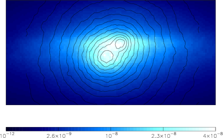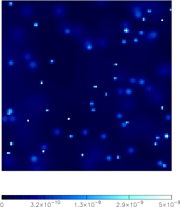
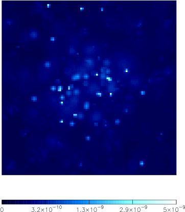
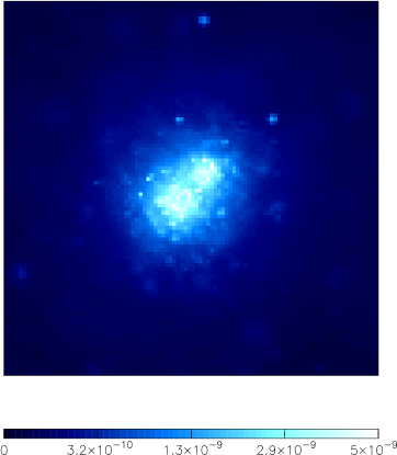
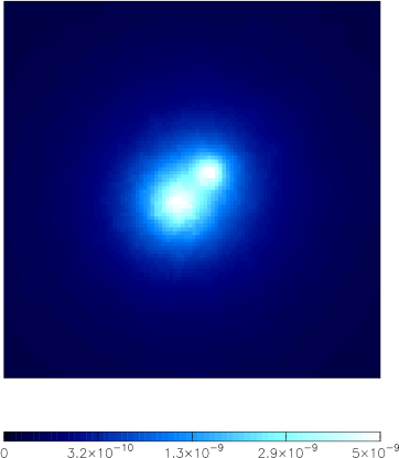
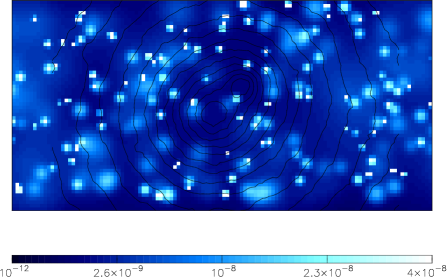
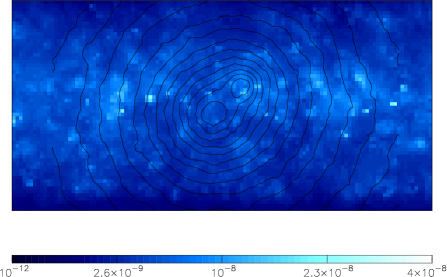
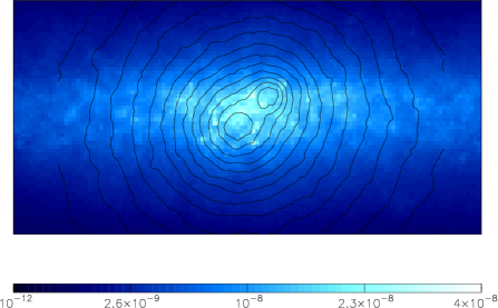
The median map can be computed by taking the median of the $L_{j}(x,y)$ or $T_{j}(x,y)$ over all iterations $j$ in the stationary part of the Markov chain. Median luminosity maps are shown in Figures 7 and 8 for the EPIC and RGS runs respectively. As can be seen in the maps from the EPIC run the particles start out as a completely random distribution but after only 100 iterations the median map exhibits clear double cluster structure. The median luminosity map of the last 800 samples in the stationary part of the Markov chain is indistinguishible from the input model. In the RGS run the clusters can be seen to be resolved approximately in the cross-dispersion direction after 1000 iterations.

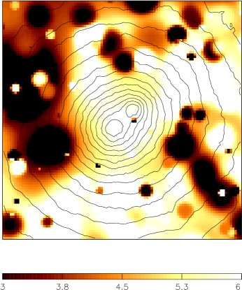
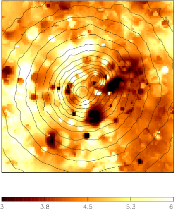
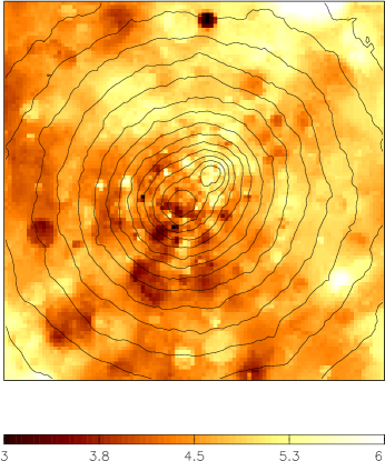
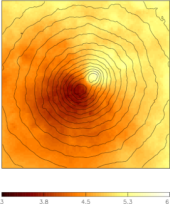
Likewise, median maps of luminosity-weighted temperature are shown in Figures 9 and 10 for XMM-Newton EPIC and RGS runs. It is clear from the sequence of plots in figure 9 that it is more difficult to estimate spatially resolved cluster plasma temperatures than a luminosity distribution. However, in the median map at iteration 1000 the two isothermal components are clearly separated; even though the map is based on the medians of very broad distributions (section 3.2) we recover approximately the input temperatures of the two components. Clearly, as seen in the maps based on the XMM-Newton RGS simulated data (Figure 10) creating spatially-resolved maps using a spectrometer alone is more difficult; however, there is spatial information there which is extracted with the SPI method.

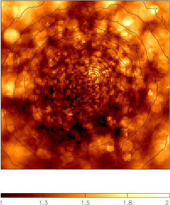
Similarly, percentile maps can also be constructed instead of just the median. The difference between say the 84th percentile and 16th percentile map gives the 1 $\sigma$ error map of a quantity in each point ($x$,$y$) with the caveat that the neighbouring pixels are highly correlated due to the underlying smooth particle structure. This means that the error map is an overestimate of the uncertainty on the pixel values. For a temperature map, for example, this procedure gives the 1 $\sigma$ error of the luminosity weighted temperature in each ($x$,$y$) bin. Such a map, created from the 800 final samples in the EPIC run, is shown in Figure 11). The map displays a 1 $\sigma$ uncertainty of kT $\sim$0.5 keV  for the bottom left (cold) component and kT $\sim$1 keV  for the top right (hot) component.

This, again, demonstrates the subtle difficulties associated with estimating high plasma temperatures given the currently available instruments. That the error on the median appears to decrease to a small value at spatial points far away from the cluster center is simply due to the fact that for those distances the simulated data contain a very small number of photons: any estimated temperature distribution will default to the applied uniform prior. The median of this uniform distribution will of course be close to the central value of the range and not vary much in the evolution of the Markov chain.

Of course, these percentile maps give only an estimate of the uncertainty of the median value. If we want to measure the width of the intrinsic range of temperatures at any given sky coordinate, should such a distribution exist, we have to do something more sophisticated. One methods to visualize parameter ranges is demonstrated in the next section.

Figure 9: $500^{\prime\prime}\times 500^{\prime\prime}$ sky-maps of ICM temperature (keV) after 1, 10, 100 and 1000 iterations centered on the double-cluster centroid. The temperature is calculated according to Eq. 24 and the median over all iterations is taken in each $5^{\prime\prime}\times 5^{\prime\prime}$ pixel. The contours show the luminosity obtained from the EPIC run after 1000 iterations. Based on data from the EPIC run.

Figure 10: $600^{\prime\prime}\times 300^{\prime\prime}$ sky-maps of ICM temperature (keV) after 1, 10, 100, 1000 iterations (top left to bottom right) for the RGS run. The contours show the luminosity obtained from the EPIC run after 1000 iterations for comparison. The particles are smeared due to the uncertainty on the position in the dispersion direction of the spectrometer.

Figure 11: $500^{\prime\prime}\times 500^{\prime\prime}$ sky-map, showing the width of the distribution for the median temperatures from iteration 200 to iteration 1000. The map depicts the difference of the 84th and 16th percentile of the distribution of the luminosity weighted temperatures for each iteration at any sky-coordinate.

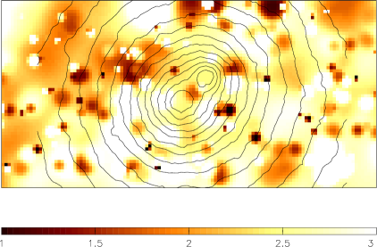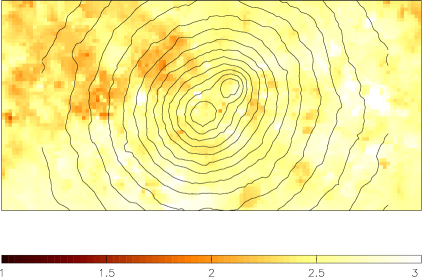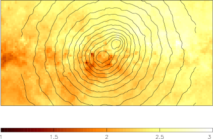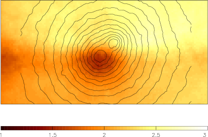3.5 Filtered Maps

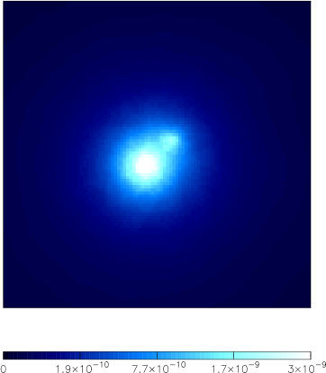
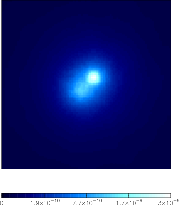
Another useful way of examining the posterior pdf of a given spatially-varying quantity is to segregate the particles into different categories before constructing the luminosity maps. A luminosity map can be constructed from particles with temperatures between say $1\times 10^{7}~{}\mbox{K}$ and $2\times 10^{7}~{}\mbox{K}$ (kT = 1-2 keV ). This can then be compared directly with other luminosity maps of other temperature ranges to study the varying spatial distribution of the different plasma temperatures. To demonstrate this two filtered luminosity maps were created, again using the final 800 samples of the EPIC chain (Figure 12). These maps were filtered for temperature ranges kT = 0-4.5 keV  (left) and kT = 4.5-9 keV  (right) respectively. This type of luminosity map, filtered on plasma temperatures, would be impossible to produce using any standard spectral analysis: it requires some kind of forward-fitted spectral-spatial multicomponent model.

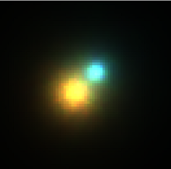
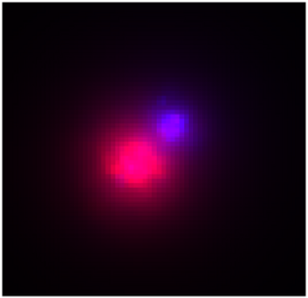
Three-color RGB maps can be computed by using filtered luminosity maps with a different temperature range for each color. In Figure 13 such an RGB map is displayed using luminosity maps filtered in three ranges of temperature of equal size. In principle, this map contains more information since it describes the width of the temperature distribution as well as the mean temperature.

Figure 12: $500^{\prime\prime}\times 500^{\prime\prime}$ sky-maps of filtered ICM luminosity using particles of temperature kT = 0-4.5 keV  (left) and kT = 4.5-9 keV  (right).

Figure 13: $300^{\prime\prime}\times 300^{\prime\prime}$ RGB sky-map of ICM luminosity (left) where each color represents the luminosity of particles in different ICM temperature ranges. Here red represents particles with kT = 0-3 keV , green; kT = 3-6 keV  and blue; kT = 6-9 keV . In the plot to the right the green component has been removed to make the difference of the hot and cold components clearer.

4 Conclusions and Future Work

To summarize and conclude:

1. Motivated by the complexity of modern X-ray data on clusters of galaxies, and the spatially- and spectrally-varying nature of both the emitting system and the instrument response, we have developed a highly flexible forward-folding analysis scheme, dubbed smoothed particle inference.

2. Deconvolution in the presence of high Poisson noise is achieved by Monte Carlo simulation of mock data and comparison of this with adaptively-binned raw counts with a two-sample likelihood function.

3. Clusters are modelled with a linear combination of Gaussian emission profiles, with variable position, size, temperature and abundance; these local parameters, and the global parameters associated with the background emission and the galactic absorption, reside in a highly multi-dimensional space which we explore with a Markov Chain Monte Carlo sampler.

4. Testing this methodology on simulated data shows that the input parameters can be recovered reliably, with precision limited by the shot noise in the Monte Carlo mock data generation.

5. SPI has been demonstrated to open up a variety of novel analysis pathways: the translation of noisy data into uncertain particle parameters brings the underlying physical distributions a significant distance closer.

Multiple avenues can be taken in extending this work further. Firstly, since we have (iteratively) propagated a complex model through the XMM instruments, it is straightforward to propagate the same model through multiple instrument responses simultaneously. Therefore, joint EPIC, RGS, Chandra, and Astro-E analyses, all of which would benefit from a careful treatment of the spatial-spectral response, may become routine. Secondly, we anticipate that simultaneous X-ray, SZ and lensing analyses could greatly benefit from a many-parametric approach such as this: simpler analyses under-use the information in the X-ray data, allowing biases to creep in. Thirdly, we expect SPI analysis of low signal-to-noise data sets, such as those obtained from X-ray cluster surveys, to be very efficient: since the computation time scales with the number of photons, analysis of simple data sets would be extremely fast. The retention of maximum information in this data regime is clearly of much interest.

Fourthly, the particle positions can also be deprojected in similar ways to standard deprojection techniques in order to model clusters in 3D: in a future paper we will show how we do this using SPI, and retaining the full 2D cluster asymmetries. Fifthly, we anticipate that a variety of hydrodynamical constraints could be applied to limit the vast parameter space volume that is being considered. To date we have used only uninformative priors, as we attempt to move from data space to particle space; the use of physical priors on the gas pressure should aid the reconstruction of the cluster plasma distribution. Finally, this work can be seen as the beginnings of a bridge to theoretical physical models of cluster formation and evolution; one can envisage such models being developed under constraints imposed by the data in something like the methodolgy outlined here. Smoothed particles sit very well in the hierarchical picture of cluster formation: we have good reason to believe that they may be the optimal basis set with which to reconstruct their images.

Appendix A Derivation of Likelihood Function

The basic datum is a number of photons in a three dimensional bin $(u_{1},u_{2},p)$. The bin size may be set by physical limits such as the extent of the CCD pixel, or be imposed given some understanding of, for example, the spectral resolution of the instrument. The simulated photons are then binned on the same grid. Assume that we have $n$ photons in the observed dataset, and have simulated $m$ photons from our model: in the $i^{\rm th}$ bin we have $E_{i}$ simulated photons, and $O_{i}$ observed photons. Since the photons falling into a set of bins will follow a multinomial distribution, we can use the usual multinomial likelihood function

$$L_{1}=n!\prod_{i}\frac{{\left(\frac{E_{i}}{m}\right)}^{O_{i}}}{O_{i}!}$$ (A1)

where we have used $\frac{E_{i}}{m}$ as a proxy for the actual probability of finding a photon in the $i$th bin. In the limit of large m, this will approach the converge to the true probability of the model.

A more sophisticated likelihood function is one that attempts to include the error induced by the Monte Carlo noise on the true probability. We then calculate, $L_{2}$, which is the product of two likelihood functions for both the detected and simulated photons (i.e. a two sample likelihood function)

$$L_{2}=n!m!\prod_{i}\frac{{{\left(\frac{O_{i}+E_{i}}{m+n}\right)}}^{O_{i}}{{\left(\frac{O_{i}+E_{i}}{m+n}\right)}}^{E_{i}}}{O_{i}!E_{i}!}$$ (A2)

where we have used $\frac{O_{i}+E_{i}}{m+n}$ as an estimate for the probability in the $i$th bin.

Another approach would be to not assume that the probability, $p_{i}$ is estimated by $\frac{O_{i}+E_{i}}{m+n}$, but instead integrate this probability distribution over a prior distribution for that probability. This is expressed as,

$$L_{3}=n!m!\prod_{i}\int\frac{p_{i}^{O_{i}}p_{i}^{E_{i}}}{O_{i}!E_{i}!}f(p_{i})dp_{i}$$ (A3)

where $f(p_{i})$ is the prior distribution. We have not, however, been able to obtain both an analytic and properly normalized expression for $L_{3}$, in the case where the numbers of simulated and observed photons are constrained to be the same. Therefore, we use $L_{2}$ and note that in the limit of large $m$ these expressions will be identical. This is indeed the case for unconstrained photon numbers where the Poisson distribution is appropriate for the likelihood of the counts in each bin. Future study, however, may develop these statistics further.

It is also possible to normalize these likelihood functions, such that they will approximately follow the $\chi^{2}$ distribution. This is done by dividing by the same expression with the probability estimates replaced by the actual number of counts. So the normalized expression for $L_{2}$ can be written as

$$L_{1}^{N}=\prod_{i}\frac{\frac{{\left(\frac{E_{i}}{m}\right)}^{O_{i}}}{O_{i}!}}{\frac{{\left(\frac{O_{i}}{n}\right)}^{O_{i}}}{O_{i}!}}=\prod_{i}\frac{{\left(\frac{E_{i}}{m}\right)}^{O_{i}}}{{\left(\frac{O_{i}}{n}\right)}^{O_{i}}}$$ (A4)

and for $L_{2}$ it is

$$L_{2N}=\prod_{i}\frac{\frac{{{\left(\frac{O_{i}+E_{i}}{m+n}\right)}}^{O_{i}}{{\left(\frac{O_{i}+E_{i}}{m+n}\right)}}^{E_{i}}}{O_{i}!E_{i}!}}{\frac{{{\left(\frac{O_{i}}{n}\right)}}^{O_{i}}{{\left(\frac{E_{i}}{m}\right)}}^{E_{i}}}{O_{i}!E_{i}!}}=\prod_{i}\frac{{{\left(\frac{O_{i}+E_{i}}{m+n}\right)}}^{O_{i}+E_{i}}}{{{\left(\frac{O_{i}}{n}\right)}}^{O_{i}}{{\left(\frac{E_{i}}{m}\right)}}^{E_{i}}}$$ (A5)

Note that $-2\log{L_{1}^{N}}$ and $-2\log{L_{2N}}$ will be distributed as $\chi^{2}$ with the number of degrees of freedom equal to the number of bins. We use $L_{2N}$ for all future analysis. In the appendix we demonstrate how this statistic approaches the two sample $\chi^{2}$ statistic that we used in the large $m$ and $n$ limit.

Following, we demonstrate how the likelihood function, we described in §2.3 approach the two sample $\chi^{2}$ distribution.

$$L_{2N}=\prod_{i}\frac{{{\left(\frac{O_{i}+E_{i}}{m+n}\right)}}^{O_{i}+E_{i}}}{{{\left(\frac{O_{i}}{n}\right)}}^{O_{i}}{{\left(\frac{E_{i}}{m}\right)}}^{E_{i}}}$$ (A6)

Note, if we take the logarithm of the above equation, we obtain

$$\log{L_{2N}}=\sum_{i}O_{i}\log{n\frac{\frac{O_{i}+E_{i}}{m+n}}{O_{i}}}+E_{i}\log{m\frac{\frac{O_{i}+E_{i}}{m+n}}{E_{i}}}.$$ (A7)

Rewriting this,

$$\log{L_{2N}}=\sum_{i}O_{i}\log{\left(1+\frac{n\frac{O_{i}+E_{i}}{m+n}-O_{i}}{O_{i}}\right)}$$ (A8)

$$+E_{i}\log{\left(1+\frac{m\frac{O_{i}+E_{i}}{m+n}-E_{i}}{E_{i}}\right)}.$$ (A9)

Expanding these around $\frac{n\frac{O_{i}+E_{i}}{m+n}-O_{i}}{O_{i}}\equiv\epsilon_{1}\approx 0$ and $\frac{m\frac{O_{i}+E_{i}}{m+n}-E_{i}}{E_{i}}\equiv\epsilon_{2}\approx 0$, we obtain

$$\log{L_{2N}}=\sum_{i}O_{i}\left(\epsilon_{1}-\frac{\epsilon_{1}^{2}}{2}\right)+E_{i}\left(\epsilon_{2}-\frac{\epsilon_{2}^{2}}{2}\right)$$ (A10)

Exponentiating this equation gives,

$$L_{2N}=\prod_{i}e^{-\frac{\left(O_{i}-n\frac{O_{i}+E_{i}}{m+n}\right)^{2}}{2O_{i}}}e^{-\frac{\left(O_{i}-n\frac{O_{i}+E_{i}}{m+n}\right)^{2}}{2O_{i}}}e^{n\frac{O_{i}+E_{i}}{m+n}-O_{i}}e^{m\frac{O_{i}+E_{i}}{m+n}-E_{i}}$$ (A11)

The last two factors multiplied together are one, so we obtain,

$$L_{2N}=\prod_{i}e^{-\frac{\left(O_{i}-n\frac{O_{i}+E_{i}}{m+n}\right)^{2}}{2O_{i}}}e^{-\frac{\left(O_{i}-n\frac{O_{i}+E_{i}}{m+n}\right)^{2}}{2E_{i}}}$$ (A12)

when both $m$ and $n$ are large. For small $\epsilon_{1}$ and $\epsilon_{2}$, this is also equivalent to

$$L_{2N}=\prod_{i}e^{-\frac{\left(O_{i}-n\frac{O_{i}+E_{i}}{m+n}\right)^{2}}{2n\frac{O_{i}+E_{i}}{m+n}}}e^{-\frac{\left(E_{i}-m\frac{O_{i}+E_{i}}{m+n}\right)^{2}}{2m\frac{O_{i}+E_{i}}{m+n}}}$$ (A13)

and this is exactly equal to

$$L_{2N}=e^{-\frac{\chi^{2}_{2S}}{2}}.$$ (A14)

where $\chi^{2}_{2S}$ is the two sample $\chi^{2}$ function that was used in Peterson, Jernigan, & Kahn (2004). Its reduced value would be close to one for a good fit.

Appendix B Test of Parameter Update Method

In order to determine if the interation sequence we used in §2.4.3 is valid and approximately obeys detailed balance we performed several simulations. We use the double isothermal beta model in §3.1 as the input simulation. We then fit this same model to the simulation instead of using the smoothed particles. In this way, the model is much simpler and only has the following 15 parameters, column density, the two temperatures, core radii, $\beta$, the positions (4 parameters), the two abudances, and overall normalizations. With this few numbers of parameters, we can update the parameters in three different ways. First, we update the parameters treating all the parameters as global parameters defined in §2.4.3. This is a proper Markov chain obeying detailed balance and all parameters are modified simulataneously in a single Markov step. Second, we update the parameters for one beta model as global parameters and the other parameters as local parameters. Third, we update all the parameters as local parameters. The second two approaches are not standard Markov chains, but essentially create small Markov chains at each iteration for some of the parameters.

Figure 14: Posterior distributions of temperature (right) and absorption (left) using three different parameter update schemes; all global (dotted), mixed global and local (thin dashed) and all local parameters (thick dashed).

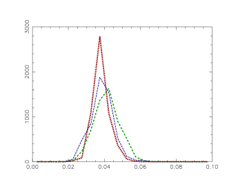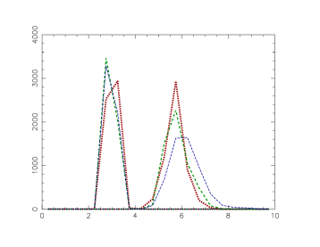
We display the posterior distributions of the temperature and absorption parameters in Figure 14. In all three simulations the posterior distribution is identical. This demonstrates that the various iteration scheme approximately obey detailed balance. This suggests that it is not critically important what scheme we use and works in the limit that the posterior distribution becomes stationary. These simulations also demonstrate that the posterior temperature distribution is smaller when the model is constrained to only consist of two temperatures than the other simulations with smoothed particles because of the simplicity of the model. The posterior distribution is smallest at low temperatures because of the nature of X-ray spectra.

References

- Andersson & Madejski (2004) Andersson, K. & Madejski, G. 2004, ApJ 607, 190.
- Andersson et al. (2006) Andersson, K. et al. 2006, in preparation.
- Arabadjis, Bautz & Garmire (2002) Arabadjis, J. S., Bautz, M. W. & Garmire, G. P. 2002, ApJ, 572, 66
- Arnaud (2001) Arnaud, M. et al. 2001, A&A 365, 80.
- Buote et al. (2003) Buote, D. A., Lewis, A. D., Brighenti, F., & Mathews, W. G. 2003, ApJ 594, 741.
- Bonamente et al. (2004) Bonamente, M., Joy, M. K., Carlstrom, J. E., Reese, E. D., & LaRoque, S. J. 2004, ApJ, 614, 56
- Cowan (1998) Cowan, G. 1998, Statistical Data Analysis, Oxford.
- Fabian, Cowie & Grindlay (1981) Fabian, A. C., Hu, E. M., Cowie, L. L., & Grindlay, J. 1981, ApJ, 248, 47
- Fabian et al. (2003) Fabian, A. C. et al. 2003, MNRAS 344, 43.
- Gilks, Richardson & Spiegelhalter (2003) Gilks, W. R. and Richardson, S. & Spiegelhalter, D. J., 1996, Markov-Chain Monte-Carlo In Practice. Chapman and Hall, Cambridge
- Hastings (1970) Hastings, W. K. 1970, Biometrika, 57, 97
- Jernigan & Vezie (1996) Jernigan, J. G. & Vezie, M. 1996, in ASP Conf. Ser. 101, Astronomical Data Analysis Software and Systems V, ed. G. H. Jacoby & J. Barnes (San Francisco: ASP), 167
- Kaastra et al. (2003) Kaastra, J. S. et al. 2003, A & A 413, 414.
- Kaastra (1992) Kaastra, J. S. 1992, An X-Ray Spectral Code for Optically Thin Plasmas (Internal SRON-Leiden Report, updated version 2.0)
- Lewis & Bridle (2002) Lewis, A. & Bridle S.L., 2002, Phys.Rev. D 66, 103511
- Liedahl, Osterheld, & Goldstein (1995) Liedahl, D. A., Osterheld, A. L., & Goldstein, W. H. 1995, ApJ, 438, L115
- McKay (2003) McKay, D.J.C., 2003, Information Theory, Inference, and Learning Algorithms Cambridge University Press
- Markevitch et al. (2000) Markevitch, M. et al., 2000, ApJ 541, 542
- Marshall et al. (2002) Marshall, P. J., Hobson, M. P., Gull, S. F, Bridle, S. L. 2002, MNRAS 335, 1037.
- Marshall et al. (2003) Marshall, P. J., Hobson, M. P., Slosar, A. 2003, MNRAS 346, 489.
- Metropolis et al. (1953) Metropolis, N., Rosenbluth, A. W., Rosenbluth, M. N., Teller, A. H., & Teller, E. 1953, J. Chem. Phys., 21, 1087
- Mewe, Gronenschild, & van den Oord (1985) Mewe, R., Gronenschild, E. H. B. M., & van den Oord, G. H. J. 1985, A&AS, 62, 197
- Mewe, Lemen, & van den Oord (1986) Mewe, R., Lemen, J. R., & van den Oord, G. H. J. 1986, A&AS, 65, 511
- Morrison & McCammon (1983) Morrison, R. & McCammon, D. 1983, ApJ, 270, 119
- Skilling (1998) Skilling, J., 1998, in Maximum Entropy and Bayesian Methods, G.Erickson, J.T.Rychert & C.Ray.Smith (eds) Kluwer Academic Publishers, Dordtrecht
- Ó’Ruanaidh & Fitzgerald (1996) Ó’Ruanaidh J. J. K., Fitzgerald W. J., 1996, Numerical Bayesian Methods Applied to Signal Processing. Springer-Verlag, New-York
- Peterson et al. (2001) Peterson, J. R. et al. 2001, A & A 365, 104.
- Peterson et al. (2003) Peterson, J. R. et al. 2003, ApJ 590, 207.
- Peterson, Jernigan, & Kahn (2004) Peterson, J. R., Jernigan, J. G., & Kahn, S. M. 2004, ApJ 615, 545.
- Peterson et al. (2006) Peterson, J. R. et al. 2006, in preparation.
- Roberts, Gelman, & Gilks (1997) Roberts, G. O., Gelman, A., & W. R. Gilks, Annals of Applied Probability 7, 110.
- Sanders et al. (2004) Sanders, J. S., Fabian, A. C., Allen, S. W., & Schmidt, R. W. 2004, MNRAS 349, 952.
- Sanderson et al. (2004) Sanderson, A. J., Finoguenov, A., Mohr, J. J. 2004, ApJ Accepted.
- Tegmark et al. (2004) Tegmark, M. et al., 2004, Phys.Rev. D 69, 103501.