First Results On Shear-Selected Clusters From the Deep Lens Survey: Optical Imaging, Spectroscopy, and X-ray Followup

Abstract

We present the first sample of galaxy clusters selected on the basis of their weak gravitational lensing shear. The shear induced by a cluster is a function of its mass profile and its redshift relative to the background galaxies being sheared; in contrast to more traditional methods of selecting clusters, shear selection does not depend on the cluster’s star formation history, baryon content, or dynamical state. Because mass is the property of clusters which provides constraints on cosmological parameters, the dependence on these other parameters could induce potentially important biases in traditionally-selected samples. Comparison of a shear-selected sample with optically and X-ray selected samples is therefore of great importance. Here we present the first step toward a new shear-selected sample: the selection of cluster candidates from the first 8.6 deg² of the 20 deg² Deep Lens Survey (DLS), and tabulation of their basic properties such as redshifts and optical and X-ray counterparts.

1 Introduction

The potential of using galaxy clusters as precision cosmological probes is by now well known (Haiman, Mohr & Holder 2001). Clusters can however be selected by a variety of methods, and the biases of the different methods are poorly understood. Traditional methods use galaxy overdensity or surface brightness enhancements in optical imaging (Postman et al. 1996, Gal et al. 2000, Gonzalez et al. 2001), perhaps including color information (Gladders & Yee 2000 and subsequent work); or X-ray emission (Rosati, Borgani & Norman 2002). Newer methods which have yet to produce sizable samples include the Sunyaev-Zel’dovich effect (SZE; Carlstrom, Holder & Reese 2002) and weak gravitational lensing (Tyson, Valdes & Wenk 1990; Schneider 1996; Wittman et al. 2001, 2003).

The types of biases which could exist are clear, even if their practical impact is not. Most methods, except X-ray, involve an integral of a density along the line of sight, making them susceptible to line-of-sight projections. However, the impact of false positives from projections can be greatly mitigated by spectroscopic followup, which is often required for a redshift in any case. X-ray selection is less sensitive to projections because the emission is proportional to the square of the local density, but that could also lead to biases due to internal substructure or asphericity. Most methods, except lensing, involve trace constituents of the cluster whose connection to the underlying predictable (and cosmologically significant) quantity, mass, is not completely understood. Optical, X-ray, and SZE selection depend on baryon content, which is a minor cluster component compared to dark matter. This alone is probably not a serious bias, because in a bottom-up structure formation scenario, large dark matter concentrations without baryons are very unlikely. However, optical selection additionally depends on star formation history, and X-ray selection depends on the heating of the intracluster medium (ICM). Weinberg & Kamionkowski (2002) predict that up to 20% of weak-lensing clusters have not yet heated their ICM to a level detectable with current X-ray missions. They predict this fraction to be independent of the signal-to-noise of the lensing detection, but increasing with redshift.

The redshift dependences also vary greatly across the methods. Optical and X-ray selection depend on the luminosity distance of the cluster and on k-corrections. SZE has the special property of being redshift-independent. This allows it to reach to very high redshift, where the cluster abundance is very sensitive to the cosmology, but it may increase the opportunities for chance projections. Lensing occupies a middle ground, with a broad sensitivity to mass at redshifts $\sim$ 0.2—0.7 for typical surveys. Clearly, no one method by itself will provide a perfect sample, and we must work to understand the biases through extensive intercomparisons. Some work has been done on optical-X-ray comparison (Donahue et al. 2001, 2002), but the advent of shear and SZE selected samples introduces a new challenge and a new opportunity to deepen our understanding.

Here we present the first shear-selected cluster sample, selected from 8.6 deg² of the Deep Lens Survey (DLS; Wittman et al. 2002). The DLS is a deep ground-based $BVR{z^{\prime}}$ imaging survey of 20 deg² with consistent good ($<0.9$${}^{\prime\prime}\,$) image quality in $R$, where the source galaxy shapes are measured. The rest of the paper is organized as follows: in Section 2, we give a brief history of shear selection; in Section 3, we describe our data and methods; in Section 4, we present the cluster candidates individually; and in Section 5, we offer a summary and discussion. Throughout, we use “cluster” to mean any mass concentration, without implying any properties of member galaxies.

2 History of Shear Selection

Tyson, Valdes & Wenk (1990) first reported the systematic alignments of background galaxies around a foreground cluster, now referred to as weak lensing. At the time, CCD fields of view were small and it was infeasible to search for new clusters with this method, limiting it to followup of already-known clusters. Tyson (1992) was the first to suggest using weak lensing to search for mass concentrations, rather than simply following up known clusters. Early work on cosmology constraints from cluster counts assumed NFW profiles for all clusters (Kruse & Schneider 1999). Bartelmann, King & Schneider (2001) then pointed out that because the profile has a big impact on detectability, cluster counts may reveal as much about dark-matter profiles as about global cosmological parameters.

However, in a larger view of things, cluster profiles are directly related to the cosmology and dark matter model. Shear-selected cluster counts are still straightforwardly derivable given the cosmological model, even if one has to perform an n-body simulation to realistically model the effects of cluster profiles. The first work in this direction was that of White, van Waerbeke & Mackey (2001), followed by Hennawi & Spergel (2004), who performed ray-tracing through a large-scale particle mesh simulation and computed the resulting “observed” mass and redshift distribution of clusters found in a mock survey. Both groups found that shear-selected samples will always have false positives, even for very high shear thresholds. These are caused by large-scale structure noise, which cannot be overcome by improved observations. Neither group addressed the feasibility of deriving constraints on cosmological parameters by including “false positives” in both observations and simulations; that is, simply measuring the abundance of shear peaks, which is easily computed from n-body simulations. Such an approach would preserve the clean comparison with theory which is the virtue of shear selection, but on the other hand, much of a cluster survey’s power to distinguish cosmologies comes from the redshift distribution. How to balance these factors to maximize the information from shear-selected clusters remains an open issue.

Meanwhile, the first claims of clusters discovered via weak lensing were published. In many of them (Erben et al. 2000; Umetsu & Futamase 2000; Clowe, Trentham & Tonry 2001; Miralles et al. 2002), the interpretation of the observations is not clear because the object causing the shear has not been identified with a redshift, without which mass and mass-to-light ratios (M/L) cannot be computed. The first shear-selected mass with a spectroscopic redshift appeared in 2001 ($z=0.27$, Wittman et al. 2001), followed in 2003 by another, an early result from the DLS ($z=0.68$, Wittman et al. 2003). The same year, Dahle et al. (2003) and Schirmer et al. (2003) each identified several shear-selected masses with redshifts roughly determined from two-color photometry ($z\sim 0.5$). Most of these clusters were serendipitous, usually near X-ray selected clusters which were the main target of the observations. A truly representative sample can only be taken from a survey of an unbiased area. The first published survey results were those of Miyazaki et al. (2002), who counted convergence peaks in a 2.1 deg² Subaru field, but attempted no followup in terms of redshifts, member galaxies, or X-ray emission.

Wittman et al. (2001) introduced the idea of tomographic confirmation. That is, the shear around a given lens must grow as a specific function of source redshift. To properly interpret a peak on a convergence map, one must confirm that the redshift dependence is as expected. Otherwise, the “shear” could be due to systematics in the data, such as optical distortion or local variations in the point-spread function. One might expect that this would also serve as a check against false positives from projections, but Hennawi & Spergel (2004) found false shear-selected candidates in their simulations which displayed perfectly sensible shear-redshift curves. It is understandable, given the broadness of the lensing redshift dependence and the imprecision of photometric redshifts, that filaments seen end-on cannot be diagnosed from the lensing information alone. Although it is not clear how often false positives remain with tomography, it is natural to examine other followup possibilities to weed out the false positives.

The use of spectroscopic or X-ray confirmation would reintroduce some of the biases of those methods, but perhaps at a much reduced level. For example, spectroscopic confirmation may be possible even for clusters with high M/L which would have escaped detection in an optical search. This approach would still fail on the extreme scenario of a pure dark matter cluster, but it seems likely that there is a continuum of M/L, and this approach at least allows us to go much further down the continuum than before. X-ray confirmation may not be foolproof, given the prediction that a significant fraction of weak lenses are X-ray dark, regardless of the signal-to-noise of the lensing detection. In fact, Weinberg & Kamionkowski (2003) argue for using the X-ray dark fraction in lensing samples as a constraint on dark energy which, unlike raw counts, is robust against uncertainties in observational thresholds.

These are open issues. In this paper, we try to shed light on the matter by providing critical new data: a shear-selected sample from real observations.

3 Cluster Selection Procedure

3.1 Optical Imaging Data

The DLS consists of five well-separated 2${}^{\circ}\times 2^{\circ}$ fields (see Table 1 for coordinates; all coordinates in this paper are J2000). The northern fields (F1 and F2) were observed using the Kitt Peak Mayall 4-m telescope and Mosaic prime-focus imager (Muller et al. 1998). The southern fields (F3 through F5) were observed with a similar setup at the Cerro Tololo Blanco 4-m telescope. The Mosaic imagers consist of a 4$\times$2 array of three-edge-buttable 2k$\times$4k CCDs, providing a 35${}^{\prime}\,$ field of view with 0.26${}^{\prime\prime}\,$ pixels and minimal gaps between the devices. Each DLS field is divided into a 3$\times$3 grid of 40${}^{\prime}\,$$\times$ 40${}^{\prime}\,$ subfields. These subfields are slightly larger than the Mosaic field of view, but are synthesized with dithers of up to 800 pixels (208${}^{\prime\prime}\,$). The primary motivation for the large dithers is to provide good sky flats.

Field	RA	DEC	l,b	E(B-V)
F1	00:53:25.3	+12:33:55	125,-50	0.06
F2	09:18:00	+30:00:00	197, 44	0.02
F3	05:20:00	-49:00:00	255,-35	0.02
F4	10:52:00	-05:00:00	257,47	0.025
F5	13:55:00	-10:00:00	328,49	0.05

Table 1: DLS field information.

The planned final depth for each subfield is twenty 600-s exposures in $B$, $V$, and ${z^{\prime}}$, and twenty 900-s exposures in $R$. The dithers are large enough to overlap adjacent subfields, providing more uniform depth at the subfield edges and good astrometric and photometric tie-ins which allow construction of a uniform catalog covering the entire 2${}^{\circ}\times 2^{\circ}$ field.

A key observing strategy of the DLS is to observe in $R$ when the seeing FWHM is $<0.9$${}^{\prime\prime}\,$, and in $BV{z^{\prime}}$ otherwise. Thus, at the end of the survey, the $R$ band imaging will have fairly uniform good resolution, as well as greater depth due to longer exposure time and greater system sensitivity in $R$. Shape measurements are thus done only in $R$ band, with $BVz$ used to provide color information for photometric redshifts. See Wittman et al. (2002) for further details regarding the survey design, field selection, etc. Note that photometric redshifts are not generally used in this paper because they were not available at the time the clusters were selected for X-ray followup, and they are not precise enough to rule out some types of projections. However, they will be used in future papers exploring tomography of these clusters, and for measuring the source redshift distribution for mass calibration.

Observing began in November 1999 at Kitt Peak, and in March 2000 at Cerro Tololo. The imaging data used for cluster selection in this paper cover 10.7 deg² in fields F2 through F5, which had reached a cumulative exposure time of at least 9000 s in $R$ as of March 2002, when the cluster sample was selected for X-ray followup. The effective area searched is somewhat less due to exclusion of edge areas (see below). $BV{z^{\prime}}$ data were not used in the selection due to significant gaps in coverage at the time of selection. However, $BV{z^{\prime}}$ data are now available, and we are able to present true-color images of each candidate below.

3.2 Image Processing

We remove instrumental artifacts such as bias, flatfield, etc., and perform astrometric calibration, in a standard way with the IRAF package mscred. See Wittman et al. (2002) for further technical details regarding these steps. We then make a stacked image of each subfield in $R$ as follows.

1. For each device in each contributing exposure, make a quick catalog of the high signal-to-noise objects. The initial step uses SExtractor (Bertin & Arnouts 1996), after which we cut on semiminor axis to eliminate cosmic rays; eliminate saturated objects; convert pixel positions to equatorial coordinates using routines from the wcstools library (Mink 2000), as SExtractor does not read the TNX coordinate system used by Mosaic; and compute the adaptive moments using the ellipto program (Bernstein & Jarvis 2002). The adaptive moments are second central moments weighted by a matched elliptical Gaussian and are equivalent to finding the best-fit elliptical Gaussian for each object. This is not used for shear measurement at this stage, but merely to aid in identification of stars, whose adaptive moments are not magnitude dependent as are the SExtractor intensity-weighted moments computed within a limiting isophote. The initial SExtractor step also produces a sky-subtracted image which will be the real input to the stacking software, dlscombine. This removes any need to match the sky levels when stacking, and also prevents the sky from becoming nonuniform during the non-flux-conserving repixelization step (below).

2. The mscred astrometric calibration is not good enough to stack images directly; we find shifts of typically $\sim$ 0.04${}^{\prime\prime}\,$ between the astrometry of overlapping exposures, which would lead to spurious stretching of galaxy shapes. Therefore we match all the catalogs in equatorial coordinates to produce a master catalog which defines the astrometry of the final stack image. All subsequent coordinate transformations are derived by matching individual exposures against this master, which reduces the offsets to zero within an uncertainty of $\sim$0.004${}^{\prime\prime}\,$. The master position of an object is simply the mean RA and DEC at which it was observed; objects observed only once (within the tolerance of 1.8${}^{\prime\prime}\,$) are dropped as being possibly spurious. The mean magnitude is also recorded.

3. Transform the master catalog positions to desired pixel coordinates in the output stack image. The coordinate system of the stack is a simple tangent plane projection with no optical distortion.

4. For each device in each exposure, determine the transformation from input pixel coordinates to output pixel coordinates. We use a third-order polynomial. Together, this and the previous two steps insure the best possible image registration, robust against small errors in the astrometric calibration of each input image. Precise registration is important, as errors could mimic spurious shear. Typical rms residuals of an input image when matched against the USNO A-1 catalog (Monet et al. 1998) are $\sim$ 0.35${}^{\prime\prime}\,$, whereas the residuals matched against the master catalog or the stacked image are $\sim$0.03${}^{\prime\prime}\,$.

5. For each device in each exposure, identify stars based on their position in the magnitude-size diagram, where size is defined in Bernstein & Jarvis (2002) as the sum of the adaptive moments $I_{xx}+I_{yy}$ times a correction factor for non-Gaussianity. Initial identification is done with an automatic algorithm which identifies the typical stellar size by looking for a peak in the size histogram, then selects the magnitude range for which there is a significant density enhancement at that size, compared to a control region at larger size. We inspect all selections, and manually adjust the selection in $\sim$5% of the exposures, typically because a few unflagged saturated stars caused the algorithm to identify a wider than necessary stellar locus. A typical diagram is shown in Figure 1, with the eight devices shown separately.

   

   Figure 1: Typical star selection scenario in $R$ band. All objects in the image are shown with lighter points, and the selected stars are shown in heavier points.

6. For each device in each exposure, analytically “undistort” the PSF adaptive moment combinations $I_{xx}-I_{yy}$, $I_{xy}$, and $I_{xx}+I_{yy}$ using the above coordinate transformation, then fit a smooth function to their spatial variation. This is mathematically equivalent to, but computationally faster than, repixelizing the image to remove the optical distortion and then measuring the PSF shape in the distortion-free coordinate system. The fitting function used is a third-order polynomial in x and y pixel coordinates. “Stars” which lie outside any of these fits by 3$\sigma$ or more are rejected as likely interloping galaxies. These fits are used to derive a PSF circularization kernel as in Fischer & Tyson (1997), although it is not applied immediately.

7. For each device in each exposure, correct the photometry in its catalog for the following effect. Pixels at the corner of the Mosaic subtend $\sim$5% more area than pixels at the center, due to optical distortion. Therefore, these pixels collect more sky photons, and objects which fall on these pixels are unfairly penalized when sky flats are applied, even though the sky appears to be flat after application. These objects will regain their lost flux when dlscombine remaps the image to the distortion free coordinate system without flux conservation. However, to correctly determine photometric offsets from the catalogs, the correction also has to be applied to any catalogs made before the remapping step.

8. Make a master photometric catalog from all the corrected catalogs, following the same rules as in step 2.

9. For each device in each exposure, derive a relative photometric offset by matching to the master catalog and computing the 3$\sigma$-clipped mean of the magnitude differences of the matching objects. In more recent versions of the pipeline, this and the previous step have been combined into an iterative search for the set of offsets which produce the most uniform master catalog. Also, all devices in a given exposure are now handled together, which provides extra robustness against wrong solutions for devices which have lost a large fraction of area to a bright star or readout problem.

The PSF-related steps are skipped for $BV{z^{\prime}}$, but otherwise the stacking procedure is the same. We do not make a single 2${}^{\circ}\times 2^{\circ}$ image because of its prohibitive file size and increased distortion due to tangent plane projection. Rather, we make 10k$\times$10k (43${}^{\prime}\,$$\times$43${}^{\prime}\,$) stacked images of each subfield/filter combination, providing 6${}^{\prime}\,$ of overlap between adjacent subfields, and combine the subfield catalogs afterward. For stacks with this footprint, many contributing exposures come from adjacent subfields. Thus, the overlap regions of the stacks do not represent independent data, but do represent the effects of differing pixelizations (each stack is a tangent projection about its center) and different large-scale PSF fits.

We then run dlscombine, which iterates over pixels in the output image, applying bad pixel masks, the PSF circularization kernel, coordinate transformations (with sinc interpolation), and photometric offsets to each relevant input image, and computes the mean of the valid contributing pixels, with a 3$\sigma$ clipping. Examination of the sky noise as a function of the number of input images reveals $\sqrt{n}$ improvement, indicating that we are successfully removing instrumental artifacts and reaching the Poisson noise limit.

An example of the performance of the Fischer & Tyson circularization kernel is shown in Figure 2. Typical ellipticity amplitudes before circularization are up to 6% with strong spatial correlations, falling to 1% or less, with very weak spatial correlations, after application of the kernel. Stacking multiple exposures further reduces correlations, as exposures separated by as little as fifteen minutes in time often have different PSF patterns. After stacking, the mean PSF ellipticity, averaged over the 43${}^{\prime}\,$ $\times$ 43${}^{\prime}\,$ area of the stack, is typically $\sim$0.1% in each component. We then apply another round of circularization to the stack, to smooth out any errors introduced by stacking errors, or by the inability of the relatively small (3$\times$3 pixel) kernel to handle large and/or highly elliptical PSFs in one pass. After this stage, the typical mean PSF ellipticity drops to $\sim$0.01% in each component, consistent with zero given the scatter among PSF stars.

Figure 2: PSF circularization of one device from one exposure (9${}^{\prime}\,$$\times$18${}^{\prime}\,$). Typical ellipticity amplitudes before circularization are up to 6% with strong spatial correlations. After circularization, this falls to 1% or less, with very weak spatial correlations, and improves further upon combining multiple exposures.

Stacks were made for all of fields F2 and F4, and contiguous portions of fields F3 (two subfields) and F5 (four subfields). The mean image quality, after all circularizations, was 0.90${}^{\prime\prime}\,$ with an rms subfield-to-subfield variation of 0.03${}^{\prime\prime}\,$. The total area covered by the imaging is 10.7 deg², before excluding edge areas as discussed below.

3.3 Convergence Maps

To make continuous convergence maps larger than the subfield size, we cataloged each subfield’s deep $R$ image separately using SExtractor, and stitched the subfield catalogs together into one supercatalog for each field, as follows. First, exclusion zones along the outer, noisy edges of the stacks were defined based on manual inspection of the image and catalog together. Subfield edges which abutted another subfield were not irregular; only the outer edges of the field required exclusion zones. Then, objects which appeared in only one subfield catalog (based on RA and DEC) were passed directly on to the final catalog. Objects in overlap regions were matched in RA and DEC and their properties subjected to consistency tests. Objects were rejected if the multiple measurements disagreed by 0.2^m or more in aperture magnitude, or by 1.0 pixel² or more in any of the three second central moments $I_{xx},I_{yy}$ or $I_{xy}$. Output statistics of the matching program were monitored to insure that relatively few objects were rejected, and that in a given overlap region, there were very few orphan objects in one subfield’s catalog but not in the others. These conditions were satisfied for all overlaps, indicating that the supercatalogs are free of gaps, duplications, and discontinuities.

At this point the supercatalogs contained $\sim$250,000 sources per square degree, with counts peaking at $R=25.5$. Adding the requirement that the adaptive moments be successfully measured by ellipto decreased the usable source density by $\sim$20%.

The supercatalogs were then filtered to remove low-redshift galaxies as well as possible given the limited information available at the time. We determined magnitude and size cuts by maximizing the detection signal-to-noise of simulated clusters as well as of the already-confirmed clusters in the real data (candidates 1 and 8 in Table 2).

The final cuts were:

• $23<R<25$. This is a typical cut used in lensing, representing a balance between removing obvious low-redshift galaxies, removing the faintest, noisiest galaxies, and retaining a large sample.

• $5.8<size<20$ pix², where size is defined above. With a PSF size of $\sim$6, this included a range of galaxies from barely resolved or even unresolved, to quite well resolved, but excluded very large foreground galaxies. We made no attempt to calibrate the shear by correcting the observed ellipticities to their pre-seeing values, as we were most interested in making a ranked list rather than imposing a physical threshold, and the seeing was considered uniform enough to fairly rank the shear peaks in the different fields against each other. This does have the effect of downweighting high-redshift clusters, whose background galaxy shears are more diluted by seeing. A retrospective seeing correction shows that this is a small effect, and has no consequences in any case because in this paper we do not compare the cluster redshift distribution with expectations from n-body simulations. The final DLS shear-selected cluster sample will be based on a shear threshold which has been corrected for the small field-to-field differences. Another potential problem with including some unresolved sources would be stellar contamination, but the ratio of galaxies to stars at these magnitude ranges and galactic latitudes is so large that in practice stars are not a significant factor.

• isophotal area $<150$ pixels. The intent of the isophotal area cut is to exclude large foreground galaxies. Although degenerate with magnitude and size cuts, the isophotal area cut had some effect in the simulations, and we therefore applied it to the data as well. In practice, this constraint removed about 10% of the galaxies which had survived the other cuts, mostly on the bright end where the limiting isophote of a galaxy could be at a large distance from its center even if the moments $I_{xx}+I_{yy}$ were small. For example, more than half the galaxies with $23<R<23.2$ were rejected by this criterion, compared to 0.5% of galaxies in the range $24.8<R<25$.

This filtering reduced the size of the catalogs by about 70%, to roughly 70,000 sources deg^-2. As a control, we cross-correlated the ellipticities of these sources with those of the stars. The result was consistent with zero at all angular scales. We then convolved the filtered catalogs with a kernel of the form

$$r^{-2}(1-\exp({-r^{2}\over 2r_{i}^{2}}))\exp({-r^{2}\over 2r_{o}^{2}})$$

where $r_{i}$ and $r_{o}$ are inner and outer cutoffs, respectively, to produce unnormalized convergence maps. This kernel is a modified version of the kernel presented in Fischer & Tyson (1997), with a Gaussian outer cutoff added to suppress noise from sources at large projected radius, where other structures are adding noise to the tangential shear field. We used $r_{i}=$4.25${}^{\prime}\,$ and $r_{o}=$50${}^{\prime}\,$. The results were pixelized onto maps with 30${}^{\prime\prime}\,$ pixels. These maps are shown in Figures 3 through 6.

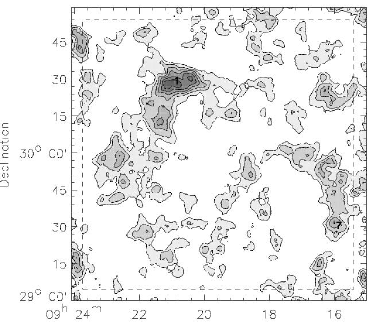
Figure 3: Convergence map for field F2, covering a full 2${}^{\circ}\times 2^{\circ}$ area. For all convergence maps in this paper, white indicates low surface mass density, black indicates highest density; north is up, east is left; dashed lines indicate the 5${}^{\prime}\,$ edge exclusion zone; and labels indicate DLS cluster number.

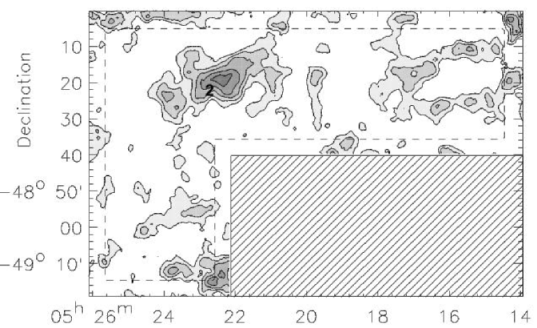
Figure 4: As for Figure 3, but for the portion of field F3 covered by the selection (1.8 deg² before edge exclusion).

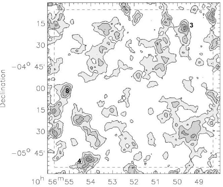
Figure 5: As for Figure 3, but for field F4 (4 deg² before edge exclusion).

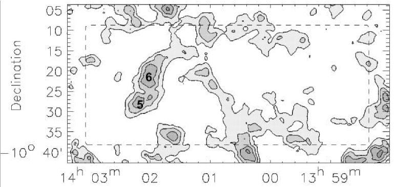
Figure 6: As for Figure 3, but for the portion of field F5 covered by the selection (0.9 deg² before edge exclusion).

3.4 Candidate Identification

We compiled a ranked list of peaks in the convergence maps and then eliminated those within 5’ of an edge, where the convergence map noise increases due to lack of input data over much of the filter footprint. The effective area searched thus decreased to 8.6 deg². This subset of the DLS area has a higher ratio of perimeter to area than does the full survey. The same edge cut applied to the full survey would yield an effective area of 16.8 deg².

We also made maps where the prefactor in Equation 1 was $r^{-1}$ rather than $r^{-2}$, though with smaller cutoff radii (1.25${}^{\prime}\,$ and 34${}^{\prime}\,$) so that the effective amount of smoothing was similar. These are akin to gravitational pseudo-potential maps rather than convergence maps. Although the two sets of maps used the same input data, one might expect shot noise and some systematic errors to propagate somewhat differently through the two algorithms. We found that for the top several candidates, the rankings yielded by the two types of maps were identical. Below that, the rankings tended to disagree by a place or two, as there were several candidates with nearly identical peak values, whose rankings were easily shuffled by a small change in the noise properties. In other words, peaks in the convergence map corresponded to peaks in the pseudo-potential map, and vice versa. We conclude that the candidates were robustly detected (see below for a quantitative estimate). The pseudo-potential maps are not presented here because they appear quite similar to the convergence maps. The final rankings were determined by the sum of the convergence and potential maps (normalized to make roughly equal contributions to the sum), as listed in Table 2.

As a control test, we repeated the entire map-making procedure using the non-tangential component of the shear. Figure 7 shows the histogram of values in the sum map for one field (F2), for the tangential component (solid outline) and the other component (dash outline). As expected, the distribution is wider in the first case, reflecting the presence of real clusters and voids. The values at the locations of the two cluster candidates in the field, candidates 1 and 7, are labeled above the solid line. The shaded area of the control histogram corresponds to a single feature right at the edge of the trimmed field. In other words, a slightly larger edge exclusion would have been better. None of our actual candidates are on the edge, so this had no effect on the sample. In summary, our candidates are above the maximum values in the control maps.

Figure 7: Histogram of values in the sum map for one field (F2), for the tangential component of shear (solid outline) and for the other component as a control (dash outline). The two candidates in this field are labeled at their sum map values, above the solid histogram. The shaded area of the control histogram represents an edge feature which would have been excluded with a slightly larger edge cut, with no effect on the actual sample.

The IAU-approved notation for DLS clusters is DLSCL JHHMM.m+DDMM, where H,D, and M refer to hours, degrees, and minutes respectively, and m refers to tenths of minutes of time. DLS JHHMMSS.ss+DDMMSS.s, where S and s refer to seconds and tenths of seconds respectively, is reserved for individual sources detected in the DLS, which have much higher positional accuracy. The sample was defined by a cutoff in the ranking rather than a cutoff in shear or signal-to-noise because the purpose here is to define a sample small enough to allow comprehensive followup with optical spectroscopy and X-ray spectro-imaging. The cutoff in Table 2 reflects the cutoff in actual X-ray followup. The final DLS shear-selected cluster sample may go further down the rankings, or equivalently to a lower shear level. As a quantitative estimate of the cutoff signal-to-noise ratio (SNR), we note that one of the lowest-ranked candidates presented below has already been published by Wittman et al. (2003) as a 3.7$\sigma$ detection.

Rank	ID	RA(J2000)	Dec(J2000)	Peak value	Field
1	DLSCL J0920.1+3029	09:20:08	+30:29:53	0.0188	2
2	DLSCL J0522.2-4820	05:22:17	-48:20:10	0.0151	3
3	DLSCL J1049.6-0417	10:49:41	-04:17:44	0.0136	4
4	DLSCL J1054.1-0549	10:54:08	-05:49:44	0.0125	4
5	DLSCL J1402.2-1028	14:02:12	-10:28:14	0.0123	5
6	DLSCL J1402.0-1019	14:02:03	-10:19:44	0.0120	5
7	DLSCL J0916.0+2931	09:16:00	+29:31:34	0.0119	2
8	DLSCL J1055.2-0503	10:55:12	-05:03:43	0.0119	4

Table 2: Ranked list of cluster candidates.

Sum of convergence map and pseudo-potential map in arbitrary units.

Note that the clusters cannot be ranked by mass without redshift information. Mass properties will be explored in a future paper; here we wish to describe the optical and X-ray counterparts and spectroscopic followup of the cluster candidates. With spectroscopic redshifts in hand, a future paper will deal with lensing masses, X-ray luminosities, and other redshift-dependent quantities. However, to set a rough mass scale to guide the reader’s expectations, we note that the mass of Candidate 8 has already been given by Wittman et al. (2003) as $8.6\pm 2.3\times 10^{14}\ (r/1\,{\rm Mpc})\ M_{\odot}$ within radius $r$, assuming a singular isothermal sphere profile. This candidate does not show significantly more shear than the lowest-ranked candidate, so it may be taken as an rough guide to the mass threshold at its redshift, $z=0.68$. This threshold changes with redshift in a way that requires knowing the source redshift distribution in detail, but as a rough guide, it is expected to fall by a factor of nearly two by redshift 0.35, and then rise again toward lower redshift. Therefore one would not expect to find a cluster in this sample with mass much less than $\sim 4\times 10^{14}\ (r/1\,{\rm Mpc})\ M_{\odot}$, although we caution that this statement is model-dependent. The same cluster provides a rough guide to the significance threshold in the current sample: roughly 4$\sigma$ based on the errors quoted in that paper.

Finally, we required a splitting criterion before making the final ranking presented in Table 2. That is, at what angular separation would a secondary peak be counted as a candidate in its own right, rather than as part of a higher-ranked candidate? Because redshift information was not available at the time, angular separation was the only criterion available. We based the decision on the practicality of X-ray followup. If several clumps could fit comfortably within the available field (formally, 8${}^{\prime}\,$ separation or less), they were considered a single candidate; otherwise, they were split. This definition of a cluster is rather frugal; the angular resolution of the convergence maps is $\sim$2${}^{\prime}\,$, and a definition based on that angular scale would have yielded more candidates above a given shear threshold. Still, 8${}^{\prime}\,$ corresponds to 3.2 Mpc (comoving) at a typical lens redshift of 0.4, so there is some justification for considering such multiple clumps to be physically associated if they are at the same redshift. When shear-selected samples are compared with n-body simulations to constrain cosmological parameters, the exact splitting criteria will matter less than the fact that the same criteria can be applied to observations and simulations without bias.

Many of the steps in this procedure have adjustable parameters, and they may be far from optimized. We would like to explore different algorithms for making convergence maps, or fitting the shear field directly for cluster models. In additon, photometric redshift information has become available since the initial selection, allowing for the possibility of a tomographic filter for the cluster selection. Future papers will explore these issues, as well as rigorously define a complete sample. The focus of this paper is the sample as defined here, which was frozen rather early in the life of the DLS to accommodate the logistics of the followup.

3.5 Followup Program

We pursued a multiwavelength followup program with these components:

• Literature search for known clusters. We searched the NASA/IPAC Extragalactic Database (NED) for known clusters within 5${}^{\prime}\,$. This generally provided little information, as most of the sky has not been searched deeply for clusters. Any overlap with a deep optical or X-ray survey would be fortuitous, so only bright, low-redshift clusters from all-sky surveys would be expected. There was only one unambiguous identification from NED, of the top-ranked candidate which happens to be Abell 781.

• X-ray spectro-imaging with the Chandra X-ray Observatory, detailed in the next subsection.

• Inspection of multicolor images, to find clustered galaxies (clustered both spatially and in color) and/or lensed arcs. One candidate had an obvious arc and has already been published (Wittman et al. 2003). We did not attempt a quantitative definition of galaxy overdensity, partly because the color information became available only gradually. Now that color information is available for all clusters, an objective optical search is underway. Based on our subjective judgement, all candidates were found to be associated closely enough with clustered galaxies to justify spectroscopic followup.

• Literature (NED) search for any galaxies within 5${}^{\prime}\,$ with spectrocopic redshifts, to make the spectroscopic followup more efficient. Specifically, field F4 overlaps the 2dF Galaxy Redshift Survey (2dFGRS catalog; Colless et al. 2001), and at several points in this paper we will refer to that survey. However, the 2dFGRS generally doesn’t go deep enough to identify redshifts of DLS clusters. With one exception, its role was limited to identifying foreground groups or providing 1—2 extra member redshifts.

• Spectroscopic redshifts. These are necessary because photometric redshifts are not precise enough to conclusively rule out line-of-sight projections. At the same time, lack of a tight cluster red sequence is not strong evidence for a projection, because many real clusters have weak red sequences. We observed with the Low-Resolution Imaging Spectrograph (LRIS, Oke et al. 1995) on the Keck I telescope on several runs: November 2000 (DLSCL J1055-0503), December 2003 (DLSCL J0916.0+2931, DLSCL J0916.0+3025) and April 2005 (DLSCL J1402.2-1028, DLSCL J1402.0-1019, DLSCL J1048.4-0411). We also used the Hydra spectrograph on the CTIO 4-m Blanco telescope in March 2004, obtaining redshifts for DLSCL J1049.6-0417 and DLSCL J0522.2-4820.

3.6 X-ray Data

X-ray imaging surveys, first with the Einstein Observatory and subsequently with ROSAT, have yielded large samples of uniformly selected galaxy clusters out to cosmologically interesting redshifts. Such surveys have provided a wealth of information on the properties of clusters and how those properties evolve with cosmic time (see e.g., Rosati, Borgani & Norman 2002). Because the X-ray emission of clusters depends on the square of the gas density, it is the observable least susceptible to line-of-sight projections, which provides an important motivation for our X-ray follow-up activities. However, another advantage of X-ray follow-up is the potential it offers us to relate the X-ray properties of our shear-selected clusters to the existing large body of knowledge on X-ray–selected clusters. A first step in this direction, presenting the X-ray luminosity–temperature relation of shear-selected clusters, is given in Hughes et al. (2005, in preparation). In the following we describe how we acquired and analyzed our X-ray followup data.

We chose pointed followup of our candidates rather than an X-ray survey of the DLS area based on practical considerations. A survey would require a great deal of telescope time and would generally be shallower than pointed observations. Pointed observations do not reveal how many X-ray–selected clusters might have been missed by shear selection, but that is not our primary interest here and indeed the literature already contains a great deal of lensing followup of X-ray–selected clusters to address that question. We concluded that the most efficient use of expensive satellite time was a pointed followup program.

Note that high angular resolution is necessary for the zero false-positive rate assumed for X-ray selection. Older X-ray facilities such as the Position Sensitive Proportional Counter onboard ROSAT with its on-axis angular resolution of 25${}^{\prime\prime}\,$ resulted in a 10% false positive rate, primarily from blends of point sources (Vikhlinin et al. 1998). Archival X-ray observations, even if deep enough, would not be suitable.

As part of this project, candidates 2–8 were observed with the Advanced CCD Imaging Spectrometer imaging array (ACIS-I) aboard the Chandra X-ray Observatory. The four ACIS-I front-side illuminated chips, as well as chip S2, were active, although for cluster detection only the four ACIS-I chips were used. This corresponds to a 16${}^{\prime}\,$ (square) field of view. As described above, this determined how we split candidates with multiple clumps.

The Chandra data were taken in timed exposure mode and events were telemetered in VFAINT format. Our first ranked candidate had been observed previously for 10 ks and its data were extracted from the archive. The other pointings were all nominally 20 ks long: after all data processing and filtering steps the individual exposure times varied from 18522 s to 20309 s. Identical reduction procedures were applied to all data sets. Background was reduced using VFAINT mode information and light curves were inspected to reject data during times of high rates. The gain map was updated, corrections for charge transfer inefficiency were applied, and events were filtered for status, grade (retaining only grades 02346), and bad pixels.

In at least half of the cases, an X-ray cluster was evident even in the raw data as an extended X-ray source near the position of the mass cluster. For consistency and in order to optimize our search for low level diffuse emission, we applied the following procedure to all observations. The photon energy range was restricted to the 0.5–2 keV band. X-ray point sources were identified and replaced with Possion noise at the level given by the average number of counts per pixel elsewhere in the image. Because of our primary interest in extended X-ray sources, we employed a very loose definition of point source and replaced any source that had even as few as 2 counts per pixel in the unblocked data. The count image was convolved with a gaussian smoothing kernel (with $\sigma=10^{\prime\prime}$), and divided by the exposure map (calculated for a photon energy of 1 keV). In all but one case, one or more extended X-ray sources appeared in the final processed image. The full extent of each source was estimated from the smoothed image and flux determination was done using this size. We present the complete list of extended X-ray sources following the description of each candidate.

4 Cluster Descriptions

In this section we present details on each cluster candidate in the Chandra sample, including redshift and optical and X-ray counterparts. In ranked order:

4.1 DLSCL J0920.1+3029 (Abell 781)

The most prominent shear-selected cluster in the sample is an Abell cluster, Abell 781, listed at $z=0.298$ by Struble & Rood (1999) and at $z=0.295$ by Bohringer et al. (2000). This is a fairly rich cluster (Abell richness class 2). Three separate clumps are resolved in the convergence map, with a maximum separation of 10${}^{\prime}\,$. Because these all fit within the ACIS-I field of view, they were counted as a single candidate. Figure 8 shows the convergence contours (green) overlaid on a BVR color composite image. We propose to name these clumps A, B, and C, from west to east (also in decreasing order of galaxy richness and X-ray flux). The position for Abell 781 given by Abell, Corwin & Olowin (1989; hereafter ACO) coincides most closely to clump A, but differs by $\sim$3${}^{\prime}\,$ in declination (the positional error quoted by ACO is 2.5${}^{\prime}\,$). Clumps A and B are identified separately in the Northern Sky Optical Cluster Survey (Gal et al. 2003) .

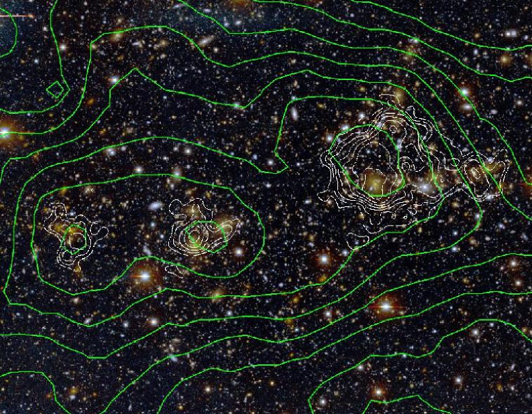
Figure 8: DLSCL J0920.1+3029 (Abell 781): convergence map (green) and X-ray (white) contours overlaid on the multiband optical imaging. North is up, east left, and the field size shown is 17${}^{\prime}\,$ diameter (4.5 Mpc at $z=0.298$). Clumps are referred to in the text as A, B, C, from west to east. For all figures, point sources have been removed from the X-ray data.

Clump A was detected in the X-ray band in the ROSAT All-Sky Survey catalog (Voges et al. 1999). Chandra observed this cluster on 3 October 2000 (Obsid #534) and in Figure 8 we plot the contours of X-ray emission from these data in white. (In all cluster figures, unless otherwise noted, X-ray contours are shown after removing point sources and smoothing). All three lensing peaks appear as extended X-ray sources, with very good positional matches to the shear peaks. In addition, with the good angular resolution of Chandra, clump A can be split into a main clump (to which we continue to refer as A) and a new clump designated D, centered 2${}^{\prime}\,$ to the west of clump A’s center.

The multiband optical imaging shows a cluster of galaxies at each clump, with very good positional and morphological agreement among galaxies, X-ray, and lensing (although in optical and lensing, the split between clumps A and D is not resolved). In addition, the order of galaxy richness closely follow the order of descending X-ray flux from A to C. However, it is clear from the colors of the galaxies that clump C is at a redshift $\sim$0.1 higher than clumps A and B. We are pursuing confirmatory spectroscopy of this clump.

In summary, Abell 781 proper consists of two main clumps separated by 6.5${}^{\prime}\,$, or 1.75 Mpc transverse at $z=0.298$. One of these clumps is resolved into two subclumps in X-ray only. Another cluster at $z\sim 0.4$ appears 4${}^{\prime}\,$ east of the eastern clump of A781 proper. Each of these three clumps is detected in lensing, X-ray, and galaxies.

A detailed paper comparing the lensing and X-ray morphologies of all clumps is in preparation. We defer the question of whether this structure should count as one, two, or three shear-selected clusters to Section 5.

4.2 DLSCL J0522.2-4820

The second-ranked candidate is 5.2${}^{\prime}\,$ from an already-known cluster, Abell 3338, but, based on the evidence we develop below, is probably not the same structure identified by ACO. NED does not contain any other clusters or galaxies with known redshift in the area. Figure 9 shows the convergence contours (green) overlaid on the optical imaging. Also marked is the nominal position of Abell 3338.

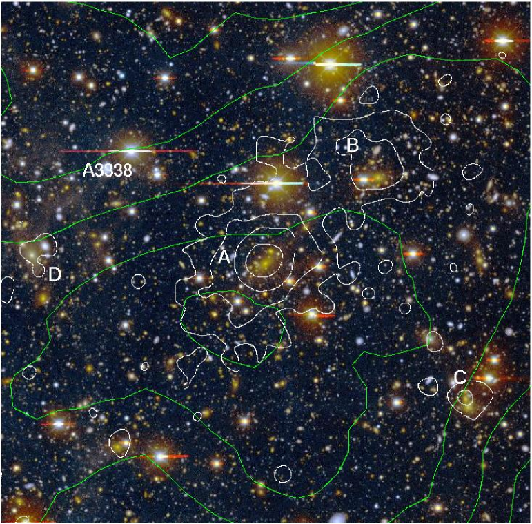
Figure 9: DLSCL J0522.2-4820: convergence map (green) and X-ray (white) contours overlaid on the multiband optical imaging. North is up, east left, and the field size shown is 12${}^{\prime}\,$ diameter (3.2 Mpc transverse at $z=0.296$). Abell 3338 is more likely associated with the lower-redshift group D than with DLSCL J0522.2-4820 (labeled A).

We obtained X-ray spectro-imaging of this cluster with Chandra on 27 June 2003 (Obsid #4208). The X-ray contours are shown in white in Figure 9. A luminous extended X-ray source appears at 05:22:15.6 -48:18:17, $\sim$2${}^{\prime}\,$north of the convergence map peak. A future paper will examine the significance and implications of offsets between positions of X-ray, convergence, and galaxy locations. Here, we are concerned with them only insofar as making a secure cross-identification. As a guide to the uncertainty in the current lensing positions, we note that the position of a different cluster, DLSCL J1054.1-0549, changed by $\sim$1${}^{\prime}\,$ when additional $R$ data became available and we restacked its subfield. Therefore, a 2${}^{\prime}\,$ displacement between the X-ray and lensing positions of this cluster is not large enough to cast significant doubt on the cross-identification.

A second, fainter, extended X-ray source is centered at 05:21:59.6 -48:16:06, 3${}^{\prime}\,$ northwest of the primary source. There is no convergence map peak at this position, but there is a definite extension in this direction from the main cluster. A third extended X-ray source appears at 05:21:47.6 -48:21:24, or 5.5${}^{\prime}\,$ southwest of the main source, and a fourth at 05:22:46.6 -48:18:04, or 5.2${}^{\prime}\,$ east of the main source. There are no convergence map peaks at these positions, nor extensions toward the positions. We label the four X-ray sources A, B, C, and D, in decreasing order of X-ray flux.

All four extended X-ray sources are coincident with clustered galaxies, with the galaxy richness generally tracking the X-ray brightness. There is no measurable positional offset between the X-ray positions and the galaxy clumps.

In March 2004 we obtained redshifts of 28 galaxies in the area around the main cluster with the Hydra instrument on the CTIO 4-m Blanco telescope. Sixteen members of clump A were identified with a mean redshift of $0.296\pm 0.001$. Three members in clump D were identified at $z=0.21$. No spectroscopy is available for clumps B and C, but the photometry suggests that they are at the same redshift as the main cluster, and are clearly at higher redshift than clump D.

Clump D is closer than any of the aforementioned positions to the nominal position of Abell 3338, with an offset of 2.5${}^{\prime}\,$, equal in size to the positional error quoted by ACO. Clump D is also at lower redshift and its galaxies have higher surface brightness than those of the other clumps. Therefore, if only one clump was detected by ACO, it should have been clump D. Furthermore, it seems unlikely that ACO conflated multiple clumps, because their position is not near the mean position of any set of clumps. Thus we suggest that clump D, not the main lensing/X-ray clump A, is Abell 3338. ACO list the redshift as 0.045, but they note that 0.045 is inconsistent with the redshift expected from the magnitudes of the cluster members. Furthermore, the redshift source is given only as a private communication, and there is no indication of how many galaxies it is based on. Therefore we believe the true redshift of Abell 3338 (clump D) is 0.21, not 0.045.

In summary, the lensing peak is coincident with a bright, extended X-ray source and a cluster of galaxies at $z=0.296$. Two secondary X-ray sources and galaxy clumps are possibly at the same redshift and simply subclumps of the main cluster. If so, they are not massive enough to cause a lensing signal, except perhaps for an extension in the direction of clump B. In addition, a cluster at lower redshift ($z=0.21$) and 5.2${}^{\prime}\,$ to the east of the main cluster, appears to be Abell 3338, which is detected in X-ray and galaxies but not on the current convergence map. Note that Abell 3338 is listed as a richness class 0 cluster. According to Briel & Henry (1993), richness class 0 Abell clusters are on the average a factor of two (four) less X-ray luminous than richness class 1 (2) Abell clusters, but with considerable scatter.

4.3 DLSCL J1049.6-0417

The third-ranked candidate has not been previously identified. Figure 10 shows the convergence contours (green) overlaid on the optical imaging.

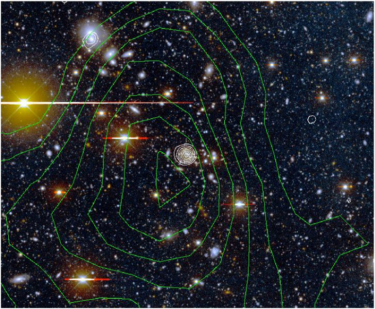
Figure 10: DLSCL J1049.6-0417: convergence map contours (green) and X-ray contours (white) overlaid on the multiband optical imaging. North is up, east left, and the field size shown is 10${}^{\prime}\,$ diameter (2.5 Mpc transverse at $z=0.267$).

The X-ray contours from Chandra spectro-imaging obtained on 2 March 2003 (Obsid #4210) are shown in white in Figure 10. A slightly extended X-ray source is centered at 10:49:37.9 -04:17:28, offset 41${}^{\prime\prime}\,$ from the convergence peak. The X-ray position is coincident with a cluster of galaxies, with no measurable positional offset between the X-ray centroid and the brightest cluster galaxy (BCG). A second, fainter extended X-ray source is visible 5${}^{\prime}\,$ to the northeast of the main cluster (10:49:50.7 -04:13:38), corresponding to a group of very large, bright galaxies.

We obtained spectroscopy of this cluster in the March 2004 Hydra run, obtaining redshifts of 19 galaxies. The mean redshift of the cluster is 0.267 $\pm 0.002$ based on seven members. The redshift of the second group and X-ray source to the northeast is $z=0.068$ based on eight members listed in the 2dFGRS. This is too low to significantly affect the convergence map, and indeed there is no deviation of the convergence contours toward this group.

4.4 DLSCL J1054.1-0549

The fourth-ranked candidate, shown in Figure 11, has not been previously identified in the literature. Chandra imaging from 3 March 2003 (Obsid #4211) reveals a single luminous extended source centered at 10:54:14.8 -05:48:50, offset $\sim$2${}^{\prime}\,$ from the convergence peak. The X-ray position is coincident with what appears to be the BCG of a cluster of galaxies. Several member spectroscopic redshifts are available from the 2dFGRS. That database lists five probable members with a mean redshift of $0.190\pm 0.001$, which we adopt for this paper.

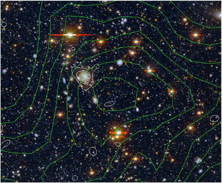
Figure 11: DLSCL J1054.1-0549: convergence map (green) and X-ray contours (white) overlaid on the multiband optical imaging. North is up, east left, and the field size shown is 10${}^{\prime}\,$ diameter (1.9 Mpc transverse at $z=0.190$).

4.5 DLSCL J1402.2-1028

The fifth-ranked candidate (Figure 12) is perhaps the most interesting. There are no previously-known clusters, or even galaxies with known redshifts, in the literature within 5${}^{\prime}\,$ of this location. The Chandra data from 19 March 2003 (ObsId #4213) reveal no significant X-ray source, with a 90% confidence upper limit of 8$\times$10^-15 erg cm^-2 s^-1 in the 0.5–2 keV band. However, the lensing position coincides with a modest group of red galaxies. Lacking a dominant BCG, the group position is not measurable to great accuracy, but its centroid is no more than 30${}^{\prime\prime}\,$ from the lensing position.

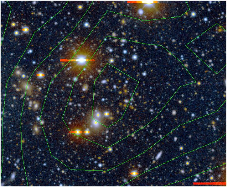
Figure 12: DLSCL J1402.2-1028: convergence map contours (green) overlaid on the multiband optical imaging. X-ray contours are omitted because there is no significant X-ray source. North is up, east left, and the field size shown is now 5${}^{\prime}\,$ diameter to better show the details described in the text.

There is also a group of lower-redshift (based on angular size, magnitude and color) galaxies 2.4${}^{\prime}\,$ to the east of the convergence map peak. At that position, the convergence map value has fallen to less than half its peak value. In contrast, the offsets of the previous clusters, although approaching 2${}^{\prime}\,$, did not involve a large drop in the convergence map value at their position. Based on that, we found the most likely cross-identification of the lensing peak to be with the higher-redshift group.

Still, with no detected X-ray emission, a line-of-sight projection is naturally suspected. Photometric redshifts indicated $z\sim 0.3$ for the low-redshift group, and $z\sim 0.5$ for the high-redshift group, so we designed one LRIS slitmask for low redshifts and another for higher redshifts. The low-redshift slitmask received less exposure time, and was shifted slightly in position, but there was a great deal of overlap in area. This allowed us to observe some galaxies through the “wrong” slitmask if the constraints on slit position in the more appropriate slitmask did not work out. There were 16 slits in the low-redshift slitmask and 19 in the high-redshift one.

We observed on 11 April 2005, and obtained 29 secure redshifts. The redshift distribution, shown in Figure 13, shows no peak. The precision of the redshifts in this dataset, based on the error in the mean of typically $\sim$6 lines, is typically $\sim$0.0005, and the bins plotted are 0.002 wide. Therefore a cluster should occupy $\sim$3 contiguous bins. Instead, pairs and triplets of galaxies are seen at many different redshifts. If this is a projection, it is of numerous nearly unrelated galaxies rather than of two readily identifiable groups.

Figure 13: DLSCL J1402.2-1028: redshift distribution. The lack of a peak, in combination with lack of X-ray emission, points to this candidate being a projection.

The current redshift data do not conclusively prove that there is no cluster. It is possible that there is a cluster at $z=0.66$ (or higher) and the targeting simply did not go deep enough to obtain many members. This seems somewhat unlikely, given that we obtained redshifts of four of the eight red galaxies in the central 50${}^{\prime\prime}\,$ bright enough for spectroscopy, and no two lie at the same redshift. Only one of these is at $z=0.66$. A second possibility is that the lower-redshift group 2.4${}^{\prime}\,$ to the east is responsible for the lensing peak despite its offset. This group has a spectroscopic redshift of 0.28 and does not appear as a large peak in Figure 13 simply because it was not considered an important target. However, on balance the evidence for either of these scenarios is weak.

4.6 DLSCL J1402.0-1019

This sixth-ranked candidate (Figure 14) consists of a prominent ridge in the convergence map with two small summits of nearly equal height on top of the ridge, one at 14:02:01 -10:19:35 and the other at 14:02:02 -10:22:44. Because these peaks are separated by much less than one ACIS-I field size, they were considered one candidate rather than two. At a lower level the ridge in the convergence map extends further south, to DLSCL J1402.2-1028. However, there is a much more clear separation between DLSCL J1402.2-1028 and DLSCL J1402.0-1019 than between the two peaks comprising DLSCL J1402.0-1019. There are no previously-known clusters, or even galaxies with known redshifts, in the literature near this location.

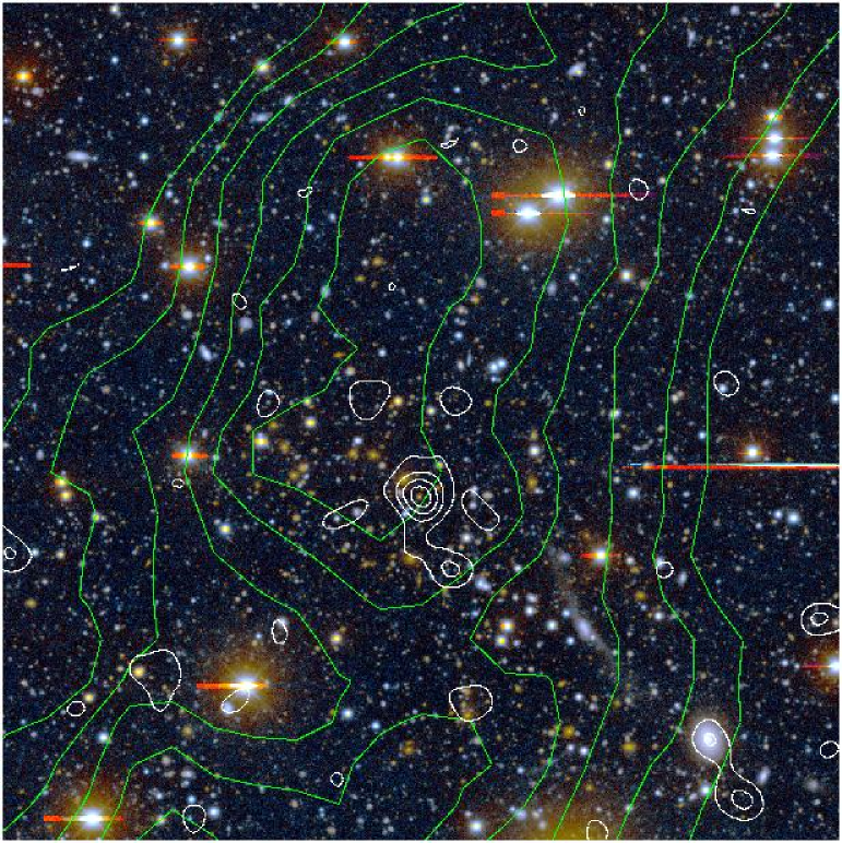
Figure 14: DLSCL J1402.0-1019: convergence map contours (green) and X-ray contours (white) overlaid on the multiband optical imaging. North is up, east left, and the field size shown is 10${}^{\prime}\,$ diameter (3.4 Mpc transverse at $z=0.427$).

The Chandra X-ray data taken 3 Sept 2003 (ObsId #4214) reveal an extended source centered at 14:01:59.7 -10:23:01.5, or 39${}^{\prime\prime}\,$ from the lensing position of the southern peak. There is no detected X-ray flux at the position of the northern peak.

The multiband optical imaging shows a modest cluster of galaxies at the southern position. This cluster lacks a dominant BCG and is fairly amorphous. Of the two brightest galaxies, the one at 14:02:00.54 -10:22:49.20 is somewhat more centrally located, so we take that as equivalent to the BCG position. This is 22${}^{\prime\prime}\,$ from the lensing position and 18${}^{\prime\prime}\,$ from the X-ray position.

We obtained Keck/LRIS redshifts of 18 galaxies in the region on 11 April 2005. We identified ten members with a mean redshift of 0.4269 $\pm$ 0.0005.

4.7 DLSCL J0916.0+2931

This candidate, on the convergence map, consists of a peak on top of a north-south ridge (Figure 15). The ridge extends $\sim$5${}^{\prime}\,$ to the south, and much further north. There is a small local maximum on the ridge $\sim$7${}^{\prime}\,$ to the north, but this bump would not have qualified as a separate candidate even had it been outside the ACIS-I field of view centered on the main peak. The literature contains no cluster or galaxy of known redshift in this region.

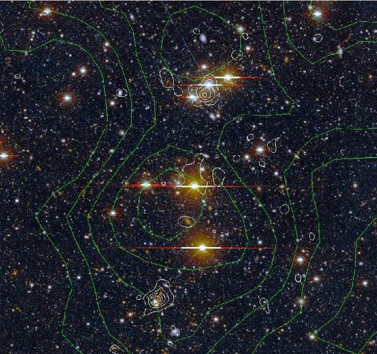
Figure 15: DLSCL J0916.0+2931: convergence map (green) and X-ray (white) contours overlaid on the multiband optical imaging. North is up, east left, and the field size shown is now 15${}^{\prime}\,$ diameter (5.7 Mpc transverse at $z=0.531$).

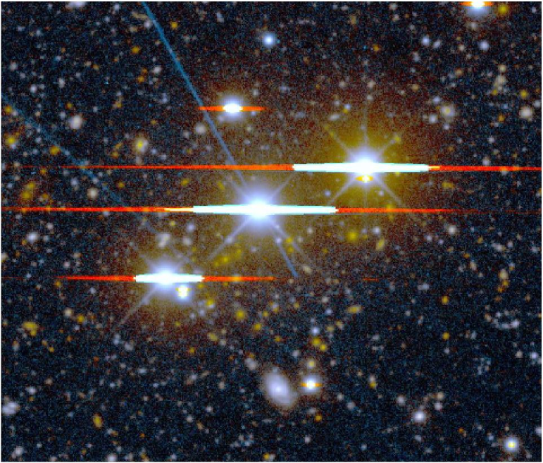
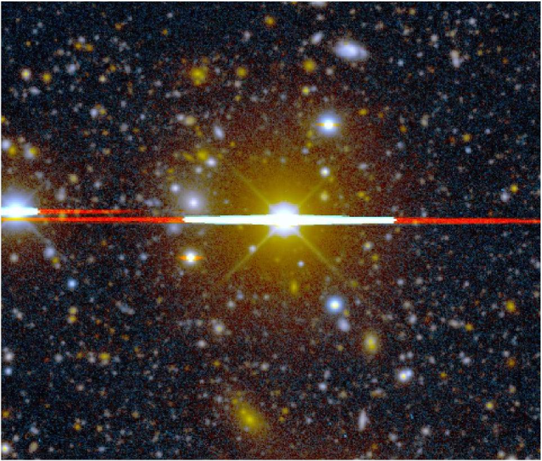
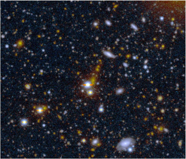
Figure 16: DLSCL J0916.0+2931: details of galaxy clumps corresponding to the northern X-ray source (top), the central X-ray source and convergence peak (middle) and the southern X-ray source (bottom). The field size is 3.5${}^{\prime}\,$ (1.3 Mpc) diameter in each case.

The Chandra data obtained on 16 December 2002 (ObsId #4209) reveal two extended X-ray sources of equal brightness. The northern one, at 09:15:51.8 +29:36:37, is on the ridge in the convergence map between the main and secondary convergence peaks, but much closer (2.4${}^{\prime}\,$) to the latter. The southern X-ray source, at 09:16:01.1 +29:27:50, lies on the southern extension in the convergence map. Fainter, more extended emission is also seen near the central convergence peak (offset 2.1${}^{\prime}\,$), with a centroid at 09:15:54.4 +29:33:16.

Close to this central cluster we detect a relatively bright X-ray point source ($F_{X}\sim 4\times 10^{-13}$ erg cm^-2 s^-1 in the 2–10 keV band), which is positionally coincident with the BL Lac object FBQS J091552.3+293324 (also designated B2 0912+29). We were careful to take account of the full extent of the Chandra point-spread-function when removing the emission from this point source.

Both brighter X-ray sources coincide with galaxy concentrations. In each case the galaxy clumps are amorphous and lacking a dominant BCG (Figure 16, top and bottom), but for the northern clump we must add the caveat that three $R\sim 12$ foreground stars severely hamper our view. In each case there is no measurable offset between the X-ray position and the galaxy clump position. There is a slightly less convincing concentration of red galaxies at the position of the fainter X-ray source, near the main lensing peak. This area, too, is partially hidden by another bright star (Figure 16, middle).

We obtained spectroscopy with Keck/LRIS on 20 December 2003, and in the southern clump found 13 members with a mean redshift of $z=0.5306\pm 0.0008$. For the northern clump, we also have a redshift of 0.53 based on two galaxies in a longslit exposure. There is no spectroscopy of the central clump as yet, but the galaxy colors and angular sizes are consistent with the same redshift.

In summary, there are two clusters of galaxies at $z=0.53$, separated by 9${}^{\prime}\,$, or 3.4 Mpc transverse in our adopted cosmology. In the center of the two is a third clump likely to be at the same redshift. The north-south separation of the three clumps is reflected in the ridge in the convergence map, which is also oriented north-south and is at the same RA. The convergence peak coincides with the central clump, but this does not automatically imply that the central clump is most massive. It may be an effect of the smoothing in the convergence maps.

4.8 DLSCL J1055.2-0503

A description of this cluster (Figure 17) has already been published by the DLS (Wittman et al. 2003), although that paper does not include the X-ray observations presented here. It had not been previously cataloged in the literature.

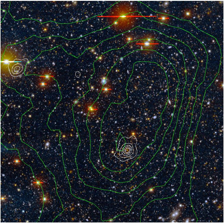
Figure 17: DLSCL J1055.2-0503: convergence map contours overlaid on the multiband optical imaging. North is up, east left, and the field size shown is 13${}^{\prime}\,$ diameter (5.6 Mpc transverse at $z=0.680$).

The Chandra data from 8 March 2003 (ObsId #4212) show an extended source at 10:55:10.1 -05:04:14, or 43${}^{\prime\prime}\,$ from the lensing position. A secondary extended X-ray source appears at 10:55:35.6 -04:59:31, or 7.2${}^{\prime}\,$ northeast of the main cluster. This does not correspond to a lensing peak, although there appears to be some extension of the lensing contours in that direction.

The multiband optical imaging shows a compact red cluster with BCG position coincident with the main X-ray position. There also appear to be strong lensing features: A large blue tangential arc, and an opposing blue radial arc (Figure 18). However, we do not have redshifts of the arcs. At the position of the second X-ray source, the optical imaging shows a concentration of red galaxies, but scattered light from a nearby bright star prevents determination of a BCG or cluster morphology.

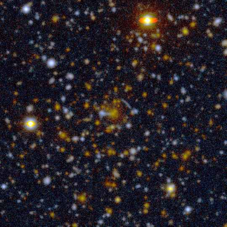
Figure 18: DLSCL J1055.2-0503: detail of the central 2.3${}^{\prime}\,$ by 1.6${}^{\prime}\,$ (1.0 by 0.7 Mpc).

We obtained Keck spectroscopy of the main cluster in November 2000, and found a mean redshift of $z=0.680\pm 0.001$ based on eleven members. We also obtained redshifts of the two galaxies closest to the second extended X-ray source in April 2005, and found both to be at $z=0.609$.

5 Summary and Discussion

5.1 Cross-identification with Previously Known Clusters

Most of these clusters were not previously known. The only unambiguous case exception is the highest-shear cluster in the survey, Abell 781. Even in that case, one of the three shear peaks—the higher-redshift one—did not correspond to a previously known cluster. This shear peak would have qualified as a candidate in its own right had we used a smaller splitting radius.

A more ambiguous case is that of the second-ranked cluster, which is near the listed position of Abell 3338. The balance of evidence is that the shear-selected cluster is not what ACO identifed as Abell 3338, but simply near it and at higher redshift. The final case in which some information existed in current databases is the fourth-ranked cluster, DLSCL J1054.1-0549, which had enough 2dFGRS redshifts to assign a cluster redshift, even though it hadn’t been identified as a group in any published work.

These facts are easily understood. The redshift sensitivity of shear selection is unlike that of any previous cluster selection technique. It is insensitive at low redshift, whereas the vast majority of clusters in current databases are precisely at low redshift because all-sky surveys have been shallow. Had the DLS overlapped with a deep pencil-beam survey, no doubt most of these clusters would have been identified by optical means. For the same reason, a literature search of known clusters inside the sample footprint, but missed by the shear selection, is unlikely to yield interesting results. Those clusters are likely to have escaped shear selection simply by virture of being too low-redshift. Abell 3338 may be a counterexample, being unselected at $z=0.21$, but there is some ambiguity regarding the identification of Abell 3338, and in any case it may have escaped shear selection because of low mass, as inferred from its low richness (class 0). For an adequate comparison of optical selection and shear selection, the optical selection must be done on the DLS data itself, which is the subject of a future paper (Margoniner et al., in preparation).

5.2 Correspondence with Extended X-ray Sources

Seven of the eight candidates exhibit detectable extended X-ray emission. The exception, DLSCL J1402.2-1028, is likely a line-of-sight projection, judging by the spectroscopy. In the other seven cases, there are positional offsets of up to 2${}^{\prime}\,$ between the X-ray sources and the shear-selected candidate positions, which may not be significant in the current set of convergence maps.

In Table 3 we present the candidate number, IAU designation, position in epoch J2000, X-ray flux $F_{X}$, statistical significance of detection (S/N), and redshifts of all the extended X-ray sources in the eight X-ray data sets. Fluxes are in the 0.5–2 keV band and have been corrected for Galactic absorption, which in all cases was modest (in the range $N_{\rm H}\sim 2-4\times 10^{20}$ atoms cm^-2). Where a candidate yielded multiple sources, the sources are ordered by $F_{X}$.

Candidate	IAU Designation	RA(J2000)	Dec(J2000)	$F_{X}$	S/N	z (source)
1	CXOU J092026+302938	9:20:26.4	30:29:39	$6.42\times 10^{-13}$	36.6	0.298 (1)
1	CXOU J092053+302800	9:20:53.0	30:28:00	$1.16\times 10^{-13}$	13.3	0.298 (1)
1	CXOU J092110+302751	9:21:10.3	30:27:52	$9.47\times 10^{-14}$	12.2	$\sim$0.4 (2)
1	CXOU J092011+302954	9:20:11.1	30:29:55	$4.98\times 10^{-14}$	9.1	0.298 (1)
2	CXOU J052215-481816	05:22:15.6	-48:18:17	$2.6\times 10^{-13}$	30.2	0.296 (3)
2	CXOU J052159-481606	05:21:59.6	-48:16:06	$5.9\times 10^{-14}$	10.4	$\sim$0.3 (2)
2	CXOU J052147-482124	05:21:47.6	-48:21:24	$8.3\times 10^{-15}$	4.9	$\sim$0.3 (2)
2	CXOU J052246-481804	05:22:46.6	-48:18:04	$4.7\times 10^{-15}$	3.3	0.21 (5)
3	CXOU J104937-041728	10:49:37.9	-04:17:29	$1.07\times 10^{-14}$	5.3	0.267 (3)
3	CXOU J104950-041338	10:49:50.7	-04:13:38	$5.6\times 10^{-15}$	3.7	0.068 (4)
4	CXOU J105414-054849	10:54:14.8	-05:48:50	$1.32\times 10^{-14}$	6.7	0.190 (4)
5	-	-	-	$<8\times 10^{-15}$	-	-
6	CXOU J140159-102301	14:01:59.7	-10:23:02	$6.6\times 10^{-15}$	4.1	0.427 (5)
7	CXOU J091551+293637	09:15:51.8	29:36:37	$1.8\times 10^{-14}$	7.6	0.53 (5)
7	CXOU J091601+292750	09:16:01.1	29:27:50	$1.8\times 10^{-14}$	7.4	0.531
7	CXOU J091554+293316	09:15:54.4	29:33:16	$7.09\times 10^{-15}$	4.6	$\sim$0.5 (2)
8	CXOU J105510-050414	10:55:10.1	-05:04:14	$2.21\times 10^{-14}$	8.7	0.680 (6)
8	CXOU J105535-045930	10:55:35.6	-04:59:31	$1.58\times 10^{-14}$	7.5	0.609 (5)

Table 3: Extended X-ray sources in Chandra followup.

This is not to imply that each X-ray source listed directly corresponds to the shear-selected candidate in its field. The relationships are not simple enough to encode in a table, so a quick recap of each candidate with multiple X-ray sources is in order:

• Each of the top three X-ray sources corresponds to its own shear peak. The fourth source is a subclump of the top source, clearly split in the X-ray but not in convergence or galaxy distribution.

• The top source corresponds to the shear-selected candidate, and the next two sources are likely to be subclumps of the same cluster, not resolved or detected separately in the current convergence maps. The fourth source (Abell 3338) is unrelated.

• The top source corresponds to the shear-selected candidate, and the second source is an unrelated low-redshift cluster with no visible effect on the convergence map.

• The faintest source listed corresponds best to the position of the convergence peak. However, the morphology of the convergence map indicates that the three subclumps were not well resolved and that the peak position may simply be the center of the smoothed distribution.

• The top source corresponds to the shear-selected candidate. The second source lies at a different redshift, but corresponds to an extension in the convergence map contours.

Extended X-ray sources with no apparent effect on their convergence maps nevertheless correspond to galaxy overdensities in each case. Excepting CXOU J104950-041338, all appear to be in the redshift range appropriate for shear selection. It is likely that they are simply not massive enough to make it into the current sample. This will be verified, assuming some mass-$L_{X}$ relation, after analyzing the full-depth DLS data (to push to a tighter shear threshold) and getting spectroscopic redshifts for all the additional X-ray sources.

There are two trends evident in Table 3. First, there is a clear correlation between X-ray flux and lensing rank. This is not surprising given that we expect each of these attributes to be linked to the more fundamental quantity, mass, but it is nevertheless reassuring that this correlation is evident even before taking the important next step of correcting for redshift effects, that is, translating $F_{X}$ into $L_{X}$ and translating shear into mass. The relation between lensing mass and X-ray luminosity (and temperature) will be extremely interesting, as it addresses the relation between observable and predictable quantities for X-ray cluster surveys. The same is true of optical M/L in the context of optical cluster selection.

Second, each of the three X-ray clusters judged to be unrelated to the main candidate is the lowest-ranked X-ray source in its target area. That is, the shear selection is not missing clusters which would be judged to be massive on the basis of an X-ray survey. Again, this statement hides some complexity, as one must first infer a mass from the X-ray data and then ask whether it should have been detected by lensing given its redshift. Nevertheless, this trend does suggest that the two methods reveal mostly overlapping subsets of the cluster population. The case which comes closest to being an exception to this trend would appear to be candidate 8 (DLSCL J1055.2-0503), where the secondary source is only $\sim 25\%$ X-ray fainter than the primary target and at a similar redshift. But the primary candidate is very near the threshold for lensing selection, so a $\sim 25\%$ less massive neighbor should be below the lensing threshold.

5.3 Correspondence with Optical Galaxy Clusters

The shear-selected clusters in this sample overwhelmingly correspond to clusters of galaxies in the optical imaging; there are no qualitatively “dark” mass concentrations. This will be further explored with quantitative measurements, such as optical mass-to-light ratios, in a future paper. Even in the case of DLSCL J1402.2-1028, which is likely to be a projection based on the X-ray and spectroscopic evidence, there appears to be a galaxy overdensity at the (two-dimensional) position of the shear-selected cluster candidate. This is a consequence of lensing and (two-dimensional) galaxy density having similar properties under line-of-sight projection, in contrast with the other two lines of evidence.

Where X-rays are detected, the position of the extended X-ray emission always matches that of the galaxy overdensity, which in many cases is different from the lensing peak position. The most likely explanation is uncertainty in the lensing position. As a guide to the uncertainty, the lensing position of DLSCL J1054.1-0549 changed by $\sim$1${}^{\prime}\,$ when additional imaging data became available and a new stack was made. Also, simulations show that for data of this depth, while the typical offset between the true and measured lens centers due to statistical noise is 20-30${}^{\prime\prime}\,$, offsets of up to 100${}^{\prime\prime}\,$ can occur. There is an additional digitization noise from the 30${}^{\prime\prime}\,$ pixels in the convergence maps. In short, offsets of up to $\sim$2${}^{\prime}\,$ may not be significant in the current dataset. This low precision will be improved when the full-depth DLS data are analyzed. In addition to the argument from the data, it is difficult to imagine a scenario giving rise to real offsets between the dark matter and the galaxies. Even in a disruptive scenario such as a merger, both dark matter and galaxies are collisionless, so they should remain together while they separate from the collisional X-ray-emitting gas.

5.4 Multiplicity

Now that redshift information is available, we revisit the candidate splitting criterion. Because redshift information provides most of the cosmology-constraining power of a cluster-counting survey, a clump at a different redshift should be counted separately. It need not have been detectable in the absence of its projected neighbor, because the comparison n-body mock survey will have cases of boosting by projected neighbors as well. Abell 781C, which probably would have been detected in the absence of its neighbors anyway, should count as a separate cluster.

Whether one splits clumps at the same redshift, such as Abell 781 A and B, is a matter of taste. Each would likely have been detected in the absence of the other. For purposes of cosmological constraints, the precise definition is not important as long as the same criteria are applied in the real survey and the mock survey from n-body simulations. The same is true for purposes of comparison to optically or X-ray selected samples.

In short, adding redshift information yields an additional candidate split from Abell 781 proper, for a total of nine candidates.

5.5 Redshift Distribution

Table 3 includes the redshifts of the cluster candidates. They cover a broad range from 0.19 to 0.68 with a median of $\sim 0.35$. This is the product of at least three factors: the source redshift distribution, which determines the lensing efficiency and thus the mass threshold as a function of lens redshift; the cluster mass function, which determines how many clusters are above the mass threshold at each redshift; and the volume probed as a function of redshift. For sources at $z=1$, the lensing efficiency peaks for lenses at $z\sim 0.35$, and is a factor of two less for lenses at $z\sim 0.1$ and $z\sim 0.7$. At lens redshifts greater than the efficiency peak, the higher mass threshold may be partially compensated by the larger volume probed, but at low redshifts, the two effects conspire to severely limit the expected number of lenses at $z\sim 0.1$. This is entirely consistent with the range seen here, which (at the risk of over-interpreting small-number statistics) seems to peak at $z\sim 0.3$ and have a long, non-negligible tail out to $z\sim 0.7$, with a sharper cutoff toward low redshifts.

This is a qualitative picture, but details will matter when the sample size grows large enough to fully characterize the observed lens redshift distribution. In particular, the sources cover a large redshift range, rather than lying in a single plane, and this will stretch the redshift range of the shear-selected clusters. Accurate characterization of the source redshift distribution, given all observational effects and cuts, will be critical for doing precision cosmology with large samples. In addition, “mass threshold” is an oversimplification of the true selection, because mass profile plays a large role in determining detectability. If mass profiles change with redshift, this will feed through to the redshift distribution. This latter issue can be addressed by comparing to mock lensing surveys of n-body simulations, so that no profile need be assumed for purposes of comparison.

5.6 Projections

Hennawi & Spergel (2004) have shown through simulations that shear-selected samples will always have false positives, even for very high shear thresholds. These are caused by large-scale structure noise, which cannot be overcome by improved observations. The same authors investigated the possibility of candidate followup with shear tomography, which examines the growth of shear with source redshift. This technique had been applied successfully by Wittman et al. (2001,2003) to constrain lens redshifts (to within $\sim 0.1$) independent of any information about the lensing cluster. Surprisingly, they found examples of false shear-selected candidates which displayed perfectly sensible shear-redshift curves. Although it is not clear how often it fails, tomography is not infallible, and it is natural to examine other followup possibilities to weed out the false positives.

Unfortunately, other forms of followup, such as optical imaging/spectroscopy of cluster member galaxies or X-ray/SZE detection of the hot intracluster medium, bring back into the sample the very biases which shear selection seeks to avoid. If nature is kind, these re-introduced biases will be small. For example, even if optically-selected samples are biased against low M/L systems, the low M/L systems which are selectable by shear only may be confirmable with spectroscopy. A bias against extremely dark systems will remain to some extent, but it will be much reduced.

If only one type of followup is pursued, spectroscopy is the natural choice. A cluster redshift, which neither X-ray nor SZE is likely to provide, is always desirable, and photometric redshifts are not accurate enough to conclusively rule out projections. For the moment, though, it is prudent to pursue as many forms of followup as possible, to confirm the very tentative conclusions here.

If one is using clusters for cosmological constraints rather than as astrophysical laboratories in their own right, there also remains the possibility of simply counting shear peaks without attaching a redshift to each one, or verifying that is a true overdensity in three dimensions. Cosmological constraints could be derived by comparison with similar mock surveys of n-body simulation. However, little work has been done in this area theoretically because most of the constraining power of cluster counts lies in the redshift distribution. Counting shear peaks without attached redshifts is a way of examining the non-Gaussian properties of the cosmic shear field, which in other contexts has been shown to supply cosmolgical constraints independent of and complementary to those provided by the Gaussian properties of the cosmic shear field (Jarvis et al. 2004).

5.7 Extensions of this Work

Many aspects of this investigation will be extended in forthcoming papers: measurement of X-ray temperatures $T_{X}$ and the $T_{X}-L_{X}$ relation; shear calibration and relations between lensing mass and $T_{X}$, $L_{X}$, and optical M/L; extension of the selection to the full area covered by the DLS; investigation of the offsets between lensing peaks and galaxy/X-ray peaks; production of a comparison optically-selected sample from the DLS imaging data; lensing tomography of the clusters, especially of DLSCL J1402.2-1028 to determine if tomography indicates that it is a projection; and shear selection with different filters, such as the tomographic matched filter suggested by Hennawi & Spergel (2004).

In the more distant future, large surveys such as LSST will find on the order of 100,000 shear-selected clusters (Tyson et al. 2003). With such massive statistics, systematics will become extremely important. Comparison to mock surveys of n-body simulations must be done very carefully to avoid introducing systematics. An efficient way of dealing with projections must be in place, as spectroscopy and X-ray followup are likely to be impractical on this scale. The modest samples produced by the DLS and other near-future surveys will provide testbeds for developing these methods.

References

- (1) Abell, G. O., Corwin, H. G., & Olowin, R. P. 1989, ApJS, 70, 1
- BKS (2001) Bartelmann, M., King, L. & Schneider, P. 2001, å378, 361
- (3) Bartelmann, M. & Schneider, P. 2001, Phys. Rep. 340, 291
- (4) Bernstein, G. M. & Jarvis, M. 2002, AJ 123, 583
- (5) Bertin, E. and Arnouts, S. 1996, A&A Supp. 117, 393
- (6) Bohringer, H. et al., 2000, ApJ129, 435
- Briel & Henry (1993) Briel, U. G., & Henry, J. P. 1993, A&A, 278, 379
- Carlstrom et al. (2002) Carlstrom, J. E., Holder, G. P., & Reese, E. D. 2002, ARA&A, 40, 643
- (9) Colless, M. et al. 2001, MNRAS 328, 1039
- Dahle et al. (2003) Dahle, H., Pedersen, K., Lilje, P. B., Maddox, S. J., & Kaiser, N. 2003, ApJ, 591, 662
- Donahue et al. (2001) Donahue, M., et al. 2001, ApJ, 552, L93
- Donahue et al. (2002) Donahue, M., et al. 2002, ApJ, 569, 689
- (13) Erben, T., van Waerbeke, L., Mellier, Y., Schneider, P., Cuillandre, J.-C., Castander, F.J. & Dantel-Fort, M. 2000, A&A 355, 23
- Fahlman, Kaiser, Squires, & Woods (1994) Fahlman, G., Kaiser, N., Squires, G., & Woods, D. 1994, ApJ, 437, 56
- Fischer (1999) Fischer, P. 1999, AJ, 117, 2024
- FT (97) Fischer, P. & Tyson, J. A. 1997, AJ 114, 14
- Gal et al. (2000) Gal, R. R., de Carvalho, R. R., Odewahn, S. C., Djorgovski, S. G., & Margoniner, V. E. 2000, AJ, 119, 12
- Gal et al. (2003) Gal, R. R., de Carvalho, R. R., Lopes, P. A. A., Djorgovski, S. G., Brunner, R. J., Mahabal, A., & Odewahn, S. C. 2003, AJ, 125, 2064
- Gladders & Yee (2000) Gladders, M. D., & Yee, H. K. C. 2000, AJ, 120, 2148
- (20) Haiman, Z., Mohr, J. & Holder, G. 2001, ApJ 553, 545
- (21) Hennawi, J. & Spergel, D. 2004, ApJ, submitted; astro-ph/0404349
- Jarvis et al. (2004) Jarvis, M., Takada, M., Jain, B., & Bernstein, G. 2004, American Astronomical Society Meeting Abstracts, 205,
- KS (99) Kruse, G. & Schneider, P. 1999, MNRAS 302, 821
- Mink (2002) Mink, D. J. 2002, ASP Conf. Ser. 281: Astronomical Data Analysis Software and Systems XI, 281, 169
- Miyazaki et al. (2002) Miyazaki, S., et al. 2002, ApJ, 580, L97
- Monet et al. (1998) Monet, D., Canzian, B., Harris, H., Reid, N., Rhodes, A., & Sell, S. 1998, VizieR Online Data Catalog, 1243, 0
- (27) Muller, G. P., Reed, R., Armandroff, T., Boroson, T. A., & Jacoby, G. H., Proc. SPIE 3355, 577, 1998
- (28) Oke, J. B., Cohen, J. G., Carr, M., Cromer, J., Dingizian, A., Harris, F. H., Labrecque, S., Lucinio, R., Schaal, W., Epps, H., & Miller, J. 1995, PASP 107, 307
- Postman et al. (1996) Postman, M., Lubin, L. M., Gunn, J. E., Oke, J. B., Hoessel, J. G., Schneider, D. P., & Christensen, J. A. 1996, AJ, 111, 615
- Rosati et al. (2002) Rosati, P., Borgani, S., & Norman, C. 2002, ARA&A, 40, 539
- Schlegel et al. (1998) Schlegel, D. J., Finkbeiner, D. P., & Davis, M. 1998, ApJ, 500, 525
- Schneider (1996) Schneider, P. 1996, MNRAS, 283, 837
- Struble & Rood (1999) Struble, M. F., & Rood, H. J. 1999, ApJS, 125, 35
- Tyson et al. (1990) Tyson, J. A., Wenk, R. A., & Valdes, F. 1990, ApJ, 349, L1
- Tyson (1992) Tyson, A. 1992, Physics Today, 45, 24
- Tyson et al. (2003) Tyson, J. A., Wittman, D. M., Hennawi, J. F., & Spergel, D. N. 2003, Nuclear Physics B Proceedings Supplements, 124, 21
- Vikhlinin et al. (1998) Vikhlinin, A., McNamara, B. R., Forman, W., Jones, C., Quintana, H., & Hornstrup, A. 1998, ApJ, 502, 558
- (38) Voges et al. 1999, A&A349, 389
- Weinberg & Kamionkowski (2002) Weinberg, N. N., & Kamionkowski, M. 2002, MNRAS, 337, 1269
- (40) Weinberg, N. & Kamionkowski, M. 2003, MNRAS, 341, 251
- White et al. (2002) White, M., van Waerbeke, L., & Mackey, J. 2002, ApJ, 575, 640
- (42) Wittman, D., et al. 2002, Proc. SPIE 4836, 73
- paper (1) Wittman, D., Margoniner, V. E., Tyson, J. A., Cohen, J. G., Becker, A. C. & Dell’Antonio, I., 2003, ApJ 597, 218 (W2003)