POWER SPECTRUM AND INTERMITTENCY OF Ly${\alpha}$ TRANSMITTED FLUX OF QSO HE2347-4342

Abstract

We have studied the power spectrum and the intermittent behavior of the fluctuations in the transmitted flux of HE2347-4342 ${\rm Ly}{\alpha}$ absorption in order to investigate if there is any discrepancy between the LCDM model with parameters given by the WMAP and observations on small scales. If the non-Gaussianity of cosmic mass field is assumed to come only from halos with an universal mass profile of the LCDM model, the non-Gaussian behavior of mass field would be effectively measured by its intermittency, because intermittency is a basic statistical feature of the cuspy structures. We have shown that the Ly$\alpha$ transmitted flux field of HE2347-4342 is significantly intermittent on small scales. With the hydrodynamic simulation, we demonstrate that the LCDM model is successful in explaining the power spectrum and intermittency of ${\rm Ly}{\alpha}$ transmitted flux. Using statistics ranging from the second to eighth order, we find no discrepancy between the LCDM model and the observed transmitted flux field, and no evidence to support the necessity of reducing the power of density perturbations relative to the standard LCDM model up to comoving scales as small as about $0.08~{}{\rm h}^{-1}~{}{\rm Mpc}$. Moreover, our simulation samples show that the intermittent exponent of the Ly$\alpha$ transmitted flux field is probably scale-dependent. This result is different from the prediction of universal mass profile with a constant index of the central cusp. The scale-dependence of the intermittent exponent indicates that the distribution of baryonic gas is decoupled from the underlying dark matter.

1 INTRODUCTION

The standard LCDM cosmogony is gaining more and more support from observations of cosmic structures, including the temperature fluctuations of cosmic background radiation, the clustering of galaxies and clusters, and the transmission flux fields of QSOs’ Ly$\alpha$ absorption spectrum. In the linear regime, the power spectrum of mass density perturbations predicted by the LCDM model is found to be consistent with observations on scales from few thousand to about 1 h^-1 Mpc (Pope et al. 2004). In the non-linear regime, N-body simulations of the standard LCDM model reveal that the mass density profile of dark matter halos is probably universal, and the cosmic mass field can be modeled as a superposition of the universal halos on various mass scales (e.g. Cooray & Sheth, 2002). This universal halo scenario has been successful in describing the second and higher order correlations of the evolved mass fields. It has also been extensively applied to model the formation and evolution of galaxies using the mass function, the universal density profile, the two-point correlation of the host halos, and the bias model of the relevant objects.

However, whether the LCDM model explains observations on sub-Mpc scales is still unclear. The universal density profile of dark matter halos given by LCDM N-body simulation is cuspy or singular, i.e., with a central density distribution given by $\rho(r)\propto r^{-\alpha}$, where $\alpha=1$ (Hernquist, 1990; Navarro et al. 1996; Jing 2000), or $3/2$ (Moore et al. 1999). However, the mass density profile given by the rotation curves of dwarf and low surface brightness galaxies generally show a soft core in their centers. The best fitted profiles are not in general as dense in the predicted cuspy center (Flores & Primack 1994; Swaters et al 2003; McGaugh et al. 2003; Zentner & Bullock 2003; Simon et al. 2004). Moreover, the observed substructures within halos are lower than predicted. These discrepancies have been used to prove that the power of density perturbations on small scales is less than the LCDM model prediction. This result has already motivated attempts to modify the LCDM model on small scales, such as the warm dark matter model, annihilating cold dark matter model (Kaplinghat et al 2000), and self-interacting dark matter model (Spergel & Steinhardt 2000).

On the other hand, the observed gravitational lensing of galaxy clusters, which yield constraints on small scale behavior of structure clustering, are found in good agreement with the LCDM model prediction (Metcalf 2004, Natarajan & Springel 2004). No reduction of small scale power is needed. Also, the $N$-body simulations show that no more than 70% of halos can be fitted by the standard universal spherical mass profile. There is considerable amount of variation in the density profile even among the halos that can be fitted by the universal mass profile (Jing 2000; Bullock et al. 2001; Ricotti 2003). The variation of the concentration parameter can be as large as a factor of two. Therefore, one needs more tests on the possible discrepancy between observations and prediction on small scales, especially using high quality samples.

In this paper, we study the small scale behavior of the cosmic field using the ${\rm Ly\alpha}$ transmitted flux of the QSO HE2347-4342, and model samples given by the hydrodynamic simulation. Along with the power spectrum, we also focus on the intermittent behavior of the field of QSO’s ${\rm Ly}{\alpha}$ transmitted flux on small scales. Roughly speaking, the intermittency of random field is characterized by strong enhancements (cuspy structures) scattered in a space with a low density background. If the cosmic mass field is given by the superposition of universal halos on various scales, all the non-Gaussian features should be from the halos. Thus, the intermittent features of QSOs’ Ly$\alpha$ transmitted flux on small scales would be effective to detect the cuspy behavior of cosmic mass field. This approach is not new. The intermittency of ${\rm Ly}\alpha$ transmitted flux has been studied using the absorption spectra of QSOs (Jamkhedkar et al. 2000; Jamkhedkar et al. 2003). The results have also been used to compare with simulations of standard LCDM model and warm dark matter model (Pando et al 2002; Feng et al. 2003). However, there are two reasons we want to revisit this topic. First, the data of HE2347-4342 ${\rm Ly}{\alpha}$ transmitted flux have higher resolution and S/N ratio than the Keck data used in previous works (Pando et al 2002; Jamkhedkar et al. 2003). Second, the newly developed hybrid cosmological hydrodynamic based on Weighted Essentially non-Oscillatory scheme (WENO) is especially effective in capturing singular and complex structures with a higher order spatial accuracy (Feng et al 2004). ${\rm Ly}{\alpha}$ transmitted flux has been extensively studied to calculate the power spectrum of mass perturbation on small scales (Croft et al. 2002; Viel et al 2004; McDonald et al. 2004).

The paper is organized as follows. In §2, we address the statistics of intermittency. Section 3 describes the data of HE2347-4342 and §4 presents the samples given by the WIGEON simulation. Sections 5 and §6 show the analysis and comparison of the power spectra and intermittent properties of observed data and simulation samples, respectively. The discussion and conclusion is presented in §7.

2 INTERMITTENT MASS FIELD

2.1 Cuspy halos and intermittency

Cuspiness of the mass density distribution can effectively be described up by density difference $\Delta\rho_{r}({\bf x})\equiv|\rho({\bf x+r})-\rho({\bf x})|$, where $r=|\bf r|$. For a field given by superposition of cuspy halos, the field is regular at most locations x, i.e. $\Delta\rho_{r}({\bf x})\rightarrow 0$, when $r\rightarrow 0$. On the other hand, cusps yield singular behavior,i.e., $\Delta\rho_{r}({\bf x})\rightarrow\infty$, when $r\rightarrow 0$. That is, the mass field consists of high spikes randomly and widely scattered in space, with a low field value between the spikes. Such spiky field is generally intermittent.

For a statistically homogeneous and isotropic random field, the probability distribution function (PDF) of density difference $\Delta\rho_{r}({\bf x})$ for a given scale $r$ has to be independent of ${\bf x}$. The existence of singular density profiles means that events with large density difference $\Delta\rho_{r}$ on small $r$ are more frequent than compared with a Gaussian field. Therefore, the PDF of $\Delta\rho_{r}$ has to be long tailed, given by the events with extremely large density difference $\Delta\rho_{r}$. The long tail would be more prominent for the PDF of smaller scales $r$. Thus, the long tail of $\Delta\rho_{r}$ PDF of the mass field is an alternative tool to probe the cuspiness of the field.

As higher order moments are sensitive to the tail of the PDF, an effective measurement of the PDF long tail is given by the so-called structure function defined as

$$S^{2n}_{r}\equiv\langle|\Delta\rho_{r}({\bf x})|^{2n}\rangle.$$ (1)

where $\langle...\rangle$ is the average over the ensemble of fields. As above mentioned, if the field is statistically homogeneous, $S^{2n}_{r}$ is independent of ${\bf x}$ and depends only on $r$. When $n=1$, we have $S^{2}_{r}=\langle|\Delta\rho_{r}({\bf x)}|^{2}\rangle$, which is the mean of the square of the density fluctuations at $r$, and therefore, $S^{2}_{r}$ actually is the power spectrum of mass density fluctuations of the field.

Intermittency of a random field is defined by the divergence of the following ratio

$$\frac{S^{2n}_{r}}{[S^{2}_{r}]^{n}}\propto\left(\frac{r}{L}\right)^{-\zeta},$$ (2)

where $L$ is the size of the sample, and $\zeta$ is called intermittent exponent. Generally, $\zeta$ is $n$- and $r$-dependent. The ratio in eq. (2) is the ${2n}^{\rm th}$ moment, $S^{2n}_{r}$, normalized by the power $S_{r}^{2}$. As $S^{2}_{r}$ measures the “width” (variance) of the PDF of $\Delta\rho_{r}(x)$, and $S^{2n}_{r}$ is sensitive to the tail of the PDF, the ratio in eq. (2) measures the fraction of events in the long tail on the scale $r$. If the exponent $\zeta$ is zero or negative, the field is regular, i.e. smooth on smaller scales. If $\zeta$ is positive, the ratio diverges as $r\rightarrow 0$, and the field is rough on small scales. In this case, the field is called to be intermittent (Gärtner & Molchanov, 1990; Zel’dovich, Ruzmaikin, & Sokoloff, 1990). Since $\Delta\rho_{r}({\bf x})\rightarrow 0$ for regular field, the $r\rightarrow 0$ asymptotic behavior of $S^{2n}_{r}/[S^{2}_{r}]^{n}$ is dominated by cuspy structures. Intermittent exponent $\zeta$ measures cuspiness of the field. If the cuspy behavior is given by $\rho(r)\propto r^{-\alpha}$ with a constant $\alpha$, the exponent $\zeta$ should also be $r$-independent.

For a Gaussian field $\rho({\bf x})$, the PDF of the density difference $\Delta\rho_{r}$ is also Gaussian. We have then

$$\frac{S^{2n}_{r}}{[S^{2}_{r}]^{n}}=(2n-1)!!.$$ (3)

This ratio is independent of scale $r$, and therefore, the intermittent exponent $\zeta=0$.

2.2 Intermittent statistics with DWT variables

The basic statistical variable in eqs. (2),  (3) is the density difference $\rho({\bf x+r})-\rho({\bf x})$, which contains the information of position ${\bf x}$ and spatial scale $r$. Therefore, it is convenient to use the statistical variables given by the discrete wavelet transform (DWT) decomposition of density field. For an 1-D field, the quantity $\rho(x+r)-\rho(x)$ in terms of DWT variables is given by the wavelet function coefficient (WFC) defined as

$$\tilde{\epsilon}_{j,l}=\int\psi_{j,l}(x)\rho(x)dx,$$ (4)

where $\psi_{j,l}(x)$ is the discrete wavelet basis function, $j$ denotes the scale $L/2^{j}$, and $l$ the spatial range $lL/2^{j}$ to $(l+1)L/2^{j}$ (Daubechies, 1992; Fang & Thews 1998). The WFC, $\tilde{\epsilon}_{j,l}$, is the density fluctuation (or difference) on scale $L/2^{j}$ at position $l$.

The structure functions in eq. (1) can then be re-written via the WFCs as (Farge at al. 1996)

$$S^{n}_{j}=\langle|\tilde{\epsilon}_{j,l}|^{n}\rangle.$$ (5)

The fair sample hypothesis allows one to calculate $S_{j}^{n}$ by using spatial averages, i.e., the average over $l$ so that

$$S^{n}_{j}=\frac{1}{2^{j}}\sum_{l=0}^{2^{j}-1}|\tilde{\epsilon}_{j,l}|^{n}.$$ (6)

For $n=2$, we have

$$S^{2}_{j}=\frac{1}{2^{j}}\sum_{l=0}^{2^{j}-1}|\tilde{\epsilon}_{j,l}|^{2}.$$ (7)

which is actually the power spectrum in the DWT modes $P_{j}\equiv S^{2}_{j}$ (Pando & Fang 1998; Fang & Feng 2000). For a Gaussian field, the Fourier power spectrum $P(n)$ is related to its DWT power spectrum $P_{j}$ by

$$P(n)=\frac{1}{L}\sum_{j=0}^{\infty}P_{j}\left|\hat{\psi}\left(\frac{n}{2^{j}}\right)\right|^{2},$$ (8)

or

$$P_{j}=\frac{1}{2^{j}}\sum_{n=-\infty}^{\infty}|\hat{\psi}(n/2^{j})|^{2}P(n),$$ (9)

where $\hat{\psi}$ is the Fourier transform of the wavelet function. This implies that the DWT power spectrum $P_{j}$ is the banded Fourier power of the flux fluctuations, and the band $j$ corresponds to the wavenumber around $k=2\pi n/L\simeq 2\pi 2^{j}/L$.

Since $r=L/2^{j}$, the intermittent exponent $\zeta$ defined by eq. (2) can be calculated by

$$\frac{S^{2n}_{j}}{[S^{2}_{j}]^{n}}\propto 2^{j\zeta}.$$ (10)

Generally, $\zeta$ depends on $n$ and $j$. The statistics of the power spectrum and intermittency are based entirely on the DWT variables. It would be easy to make a uniform comparison between model predictions and observations with statistics on second and higher orders.

3 DATA OF HE2347-4342

The data used in our analysis is the transmitted flux of the ${\rm Ly}\alpha$ absorption spectrum of QSO HE2347-4342 ($z=2.885$, $V=16.1$). The optical echelle spectra were obtained at the ESO VLT UVES on 2001 November 23-24. The details on HE2347-4342 optical spectra have been described in Zheng et al 2004. The VLT data cover the wavelength range between 3600 and 4800 Å, which corresponds to the entire ${\rm Ly}\alpha$ wavelength range studied with FUSE from $z=2.0$ to $2.9$. Using IRAF tasks designed for echelle data, a normalized spectrum was obtained. The spectrum has $24000$ points with resolution $\delta\lambda\simeq 0.05$ Å. The data are given in the form of pixels with wavelength $\lambda$, flux $F$ and noise $\sigma$. In terms of the local velocity the resolution is $dv\simeq 3.5$ km s^-1. The S/N ratio of the spectrum is about $110$ per 0.1 Å bin at 4700 Å, and about $46$ at 3850 Å. This is respectively $\sim$ $2.5$ and $10$ times of the data of Keck echelle spectrum used in Feng et al 2003.

For our purpose, the useful wavelength region is from ${\rm Ly}\beta$ absorption to the ${\rm Ly}\alpha$ emission, excluding a region close to the quasar to avoid proximity effects. Below 3984 Å ${\rm Ly}\beta$ absorption starts to appear. Therefore, we take the range from $3986.01-4395.600$ Å, corresponding to redshift from $2.278$ to $2.615$. In this wavelength range, the mean transmission $\langle e^{-\tau}\rangle$ is $0.796$. This redshift range contains about 2¹³ pixels. The size of a cell on the DWT scale $j$ corresponds to $N=2^{13-j}$ pixels. The distance between $N$ pixels in the units of the local velocity scale is given by $\delta v=2c[1-\exp(-Ndv/2c)]$ km s^-1, corresponding to comoving scale $D=(\delta v/H_{0})[\Omega_{m}(1+z_{m})^{3}+\Omega_{\Lambda}]^{-1/2}$.

Metal lines are a major cause of contamination in the spectra. But the doppler width of metal lines are generally narrow with $\delta v\leq~{}20~{}{\rm km~{}s^{-1}}$. In this paper, we restrict our analysis only to scales $\delta v\geq 30~{}{\rm km~{}s^{-1}}$ where contamination due to metal lines is low (Hu et al 1995; Boskenberg et al 2003; Kim, et al. 2004).

4 HYDRODYNAMIC SIMULATION

The simulation uses the newly developed hybrid cosmological hydrodynamic codes based on the Weighted Essentially Non-Oscillatory (WENO) scheme (Harten et al. 1987; Liu et al. 1994; Jiang & Shu 1996; Shu 1998; Fedkiw et al. 2003; Shu 2003). We will name this code as WIGEON, Weno for Intergalactic medium and Galaxy Evolution and formatiON. For details of the numerical method and tests, we refer to Feng et al.(2004). The simulation sample we analyze here is actually the same as those used in our previous papers on the statistical study of temperature, entropy, baryonic fraction and velocity fields of intergalactic medium (He et al, 2004; He et al. 2005; Kim et al. 2005). It was performed in a cubic box of side length 12 h^-1 Mpc with a 192³ grid and an equal number of dark matter particles. The cosmogony is the standard LCDM model specified by the density parameter $\Omega_{m}=0.3$, the baryon density $\Omega_{b}=0.047$, the cosmological constant $\Omega_{\Lambda}=0.7$, the Hubble constant $h=0.7$, the shape factor $\Gamma=\Omega_{m}h\exp[-\Omega_{b}(1+\sqrt{2h}/\Omega_{m})]=0.166$, and the rms mass fluctuations in spheres of $8h^{-1}$Mpc, $\sigma_{8}=0.9$. The ratio of specific heats is $\gamma=5/3$. Since the shock heating of cosmic gas is significant (He et al 2004), the resolution of the simulation should be less than the thickness of the shock, which is of the order of the dissipation length, i.e., the Jeans diffusion $\sim 0.1-0.3$ h^-1 Mpc for redshifts $z<4$ (Bi et al. 2003). The size of the grid is $12/192=33/2^{8}=0.063$ h^-1 Mpc. Therefore, the resolution of our simulation is sufficient to capture shocks.

Atomic processes including ionization, radiative cooling and heating are modelled as in Cen (1996) in a primeval plasma of hydrogen and helium of composition ($X=0.76$, $Y=0.24$). The uniform UV-background of ionizing photons is assumed to have a power-law spectrum of the form $J(\nu)=J_{21}\times 10^{-21}(\nu/\nu_{HI})^{-\alpha}$ergs^-1cm^-2sr^-1Hz^-1, with $\alpha=1$, where the photo ionizing flux is normalized by parameter $J_{21}$ at the Lyman limit frequency $\nu_{HI}$, and is suddenly switched on at $z\sim 6$ to heat the gas and re-ionize the universe.

One-dimensional fields are extracted along randomly selecting lines of sight in the simulation box. The density, temperature and velocity of the neutral gas fraction on grids are Gaussian smoothed using FFT techniques which form the fundamental data set. The one-dimensional grid containing the physical quantities is further interpolated by a cubic spline. Using this one-dimensional grid, the optical depth $\tau$ is then obtained by integrating in real space and we include the effect of the peculiar velocity and convolve with Voigt thermal broadening. To have a fair comparison with observed spectra, $\tau$ was Gaussian smoothed to match with the spectral resolutions of observation. The transmitted flux $F=\exp(-\tau)$ is normalized such that the mean flux decrement in the spectra match with observations.

Each mock spectrum is sampled on a $2^{10}$ grid with the same spectral resolution as the observation. As the corresponding comoving scale for $2^{10}$ pixels is larger than the simulation box size, we replicate the sample periodically. To achieve the greatest statistical independence, we randomly change the direction of line of sight while crossing the boundary of the simulation box. By the way, 1000 mock spectra are generated.

5 POWER SPECTRUM OF THE TRANSMITTED FLUX OF HE2347-4342

5.1 Treatment of unwanted modes

In order to calculate the DWT power spectrum [eq. (7)] of the transmitted flux of HE2347-4342, we should properly treat unwanted data, including the pixels without data, contamination of metal lines etc. Although the $S/N$ is high on an average, it is as low as about 1 for some pixels, such as pixels with negative flux. We must reduce the uncertainty given by low S/N pixels. In the DWT analysis, the conventional technique of reducing these uncertainties is given by the algorithm of DWT denoising by thresholding (Donoho 1995) or conditional-counting, (Jamkhedkar et al. 2003) as follows

1. Calculate the SFCs of both transmission $F(x)$ and noise $\sigma(x)$, i.e.

   $$\epsilon^{F}_{jl}=\int F(x)\phi_{jl}(x)dx,\hskip 8.53581pt\epsilon^{N}_{jl}=\int\sigma(x)\phi_{jl}(x)dx.$$ (11)

2. Identify an unwanted mode $(j,l)$ using the threshold condition

   $$\left|\frac{\epsilon^{F}_{jl}}{\epsilon^{N}_{jl}}\right|<f$$ (12)

   where $f$ is a constant. This condition flags all modes with S/N less than $f$. We can also flag modes dominated by metal lines.

3. Since all the statistical quantities in the DWT representation are based on an average over the modes $(j,l)$, we will skip all the flagged modes while computing these averages, i.e. the average is over the un-flagged modes $N(f)$ only.

With this method, no rejoining and smoothing of the data are needed. The condition in eq. (12) is applied on each scale $j$, and therefore the unwanted modes are flagged on a scale-by-scale basis. Generally, for scale $j$, $N(f)\leq 2^{j}$. If the size of an unwanted data segment is $R$, condition in eq. (12) only flags modes $(j,l)$ on scales less than or comparable to $R$. We also flag two modes around each unwanted mode to reduce any boundary effects of the chunks. With the conditional-counting method, we can still calculate the power spectrum by the estimators of eq. (7), but the average is not over all modes $l$, but over the un-flagged modes only.

5.2 Power spectrum of the DWT modes

We calculate the power spectrum of the transmitted flux fluctuations, $\Delta F=F(\lambda)-\langle F(\lambda)\rangle$, of HE2347-4342. To consider the correction of the noise on eq. (7), the power spectrum of transmitted flux is given by (Pando & Fang 1998b; Fang & Feng 2000; Jamkhedkar, Bi, & Fang, 2001)

$$P_{j}=\frac{1}{2^{j}}\sum_{l=0}^{N(f)}(\tilde{\epsilon}^{F}_{jl})^{2}-\frac{1}{2^{j}}\sum_{l=0}^{N(f)}(\tilde{\epsilon}^{n}_{jl})^{2}.$$ (13)

The first term on the r.h.s. of eq. (13) is the same as eq. (7), in which the wavelet coefficients (WFC) $\tilde{\epsilon}^{F}_{jl}$ are given by

$$\tilde{\epsilon}^{F}_{jl}=\int F(x)\psi_{jl}(x)dx.$$ (14)

The second term on the r.h.s. of eq.(13) is due to the noise field $\sigma(\lambda)$ and is calculated by

$$(\tilde{\epsilon}^{n}_{jl})^{2}=\int\sigma^{2}(x)\psi_{jl}^{2}(x)dx.$$ (15)

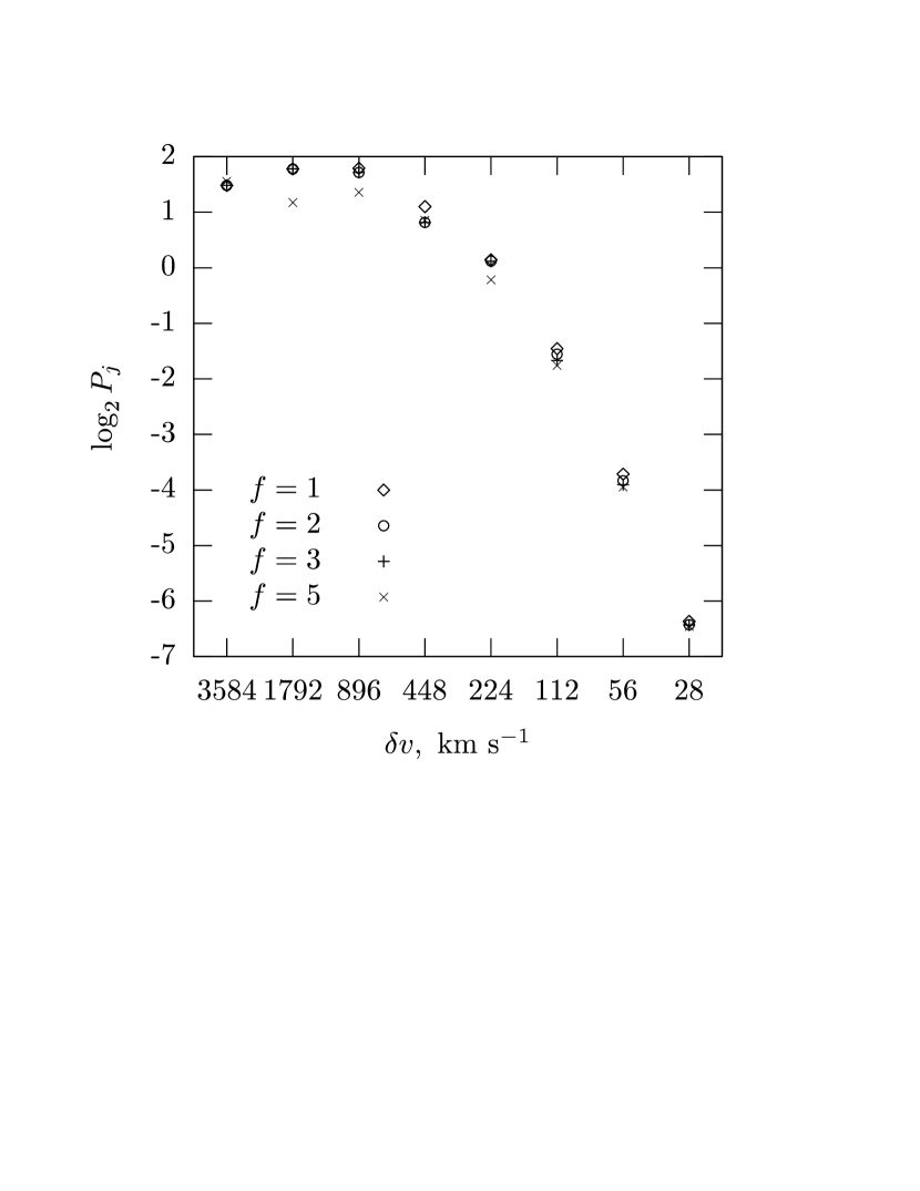
Figure 1 plots the results of the DWT power spectrum, in which the parameter $f$ is taken to be 1, 2, 3 and 5. At the first glance, the conditional-counting of eq. (12) would seem to preferentially drop modes in the low transmission regions, and power spectrum eq. (13) should be $f$-dependent. However, Figure 1 shows that the power spectrum $P_{j}$ is independent of $f$ on entire the scale range considered for $f=1$ to 5. This can be seen from eq. (13), which shows that the contribution to the power $P_{j}$ given by mode $(j,l)$ is $(\tilde{\epsilon}^{F}_{jl})^{2}-(\tilde{\epsilon}^{n}_{jl})^{2}$. The noise substraction term $(\tilde{\epsilon}^{n}_{jl})^{2}$ guarantees that the contribution of modes with small ratio $S/N$ to $P_{j}$ is always small or negligible. For instance, the modes with negative flux, i.e., the modes with flux having the same order of magnitude as noise, the two terms $(\tilde{\epsilon}^{F}_{jl})^{2}$ and $(\tilde{\epsilon}^{n}_{jl})^{2}$ statistically cancel each other. Thus, all the dropped modes have a very small or negligible contribution to $P_{j}$ regardless the parameter $f$. Denoising by thresholding or conditional-counting is reliable.

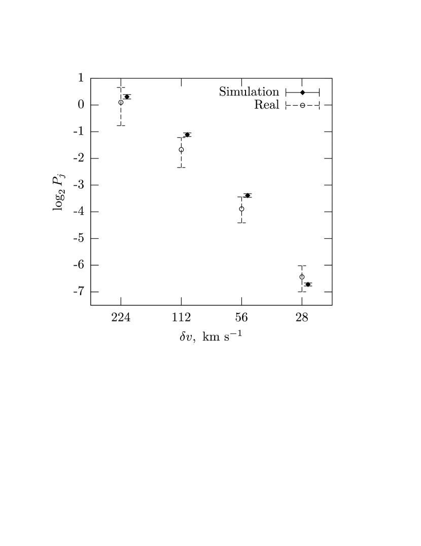
Figure 2 compares the DWT power spectra measured in the mock samples and the observed data. We take the same parameter $f=3$ for both real data and mock samples. The error bars of $P_{j}$ are the maximum and minimum range of $P_{j}$ from bootstrap re-sampling. Since the PDF of $\tilde{\epsilon}^{F}_{jl}$ is highly non-Gaussian (§5.1), a reasonable estimation of the errors for the average over the ensemble of $\tilde{\epsilon}^{F}_{jl}$ is given by bootstrap re-sampling (Jamkhedkar et al 2003). That is, for observed sample, the bootstrap re-sampling is done on the set of $N(f)$ data for each scale $j$, and for the simulation samples the bootstrap re-sampling is on the set of $N_{sim}(f)$ data from the 1000 simulation samples. The error bar is calculated thus. For a data set with $N$ points, $N$ realizations or data sets are created by drawing points from the original set with replacement. The average is calculated over the $N$ realizations. The power spectrum is calculated on the scales from $\delta v=224$ to 28 km s^-1, corresponding to comoving scale $0.63-0.079$ h^-1 Mpc in the LCDM model. The error bars for the real data are given by the maximum and minimum of bootstrap re-sampling. Figure 2 shows that simulation samples basically are in agreement with observations on the scales considered. Particularly, no discrepancy has been found even on the smallest scale $\delta v=28~{}{\rm km~{}s^{-1}}$ or length scale $D=0.079$ h^-1 Mpc.

6 INTERMITTENT BEHAVIOR

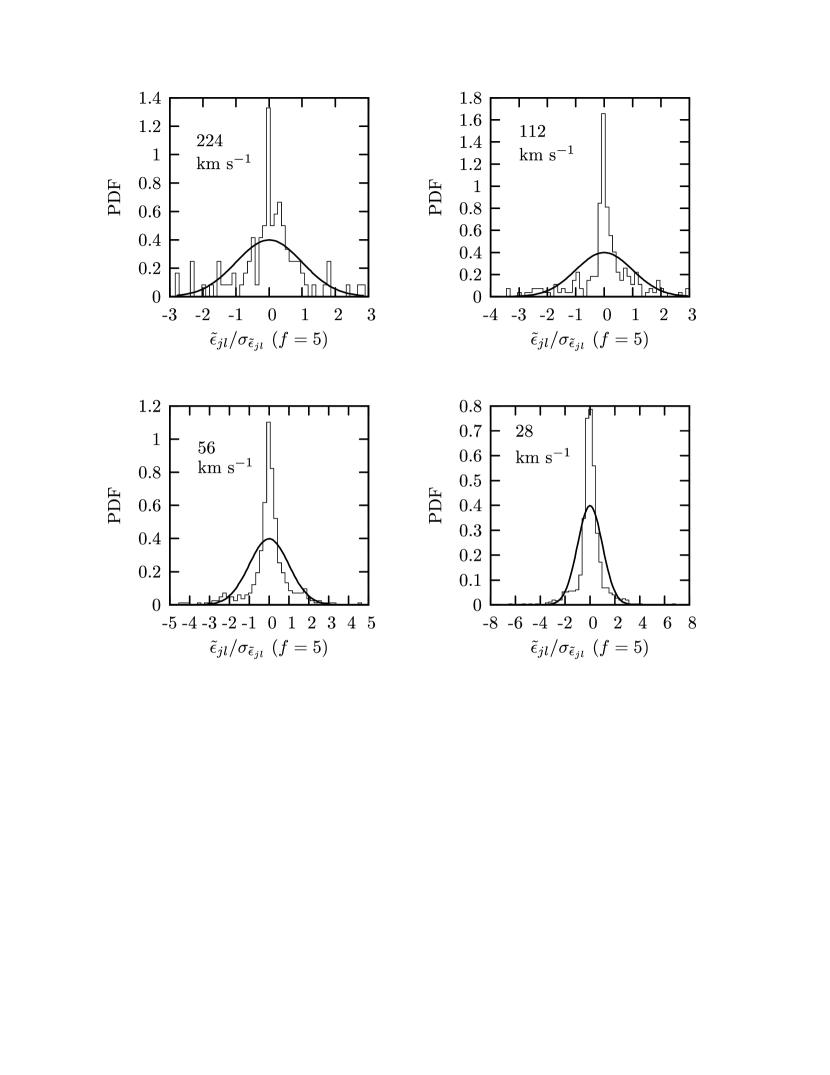
6.1 PDF of $\tilde{\epsilon}^{F}_{jl}$

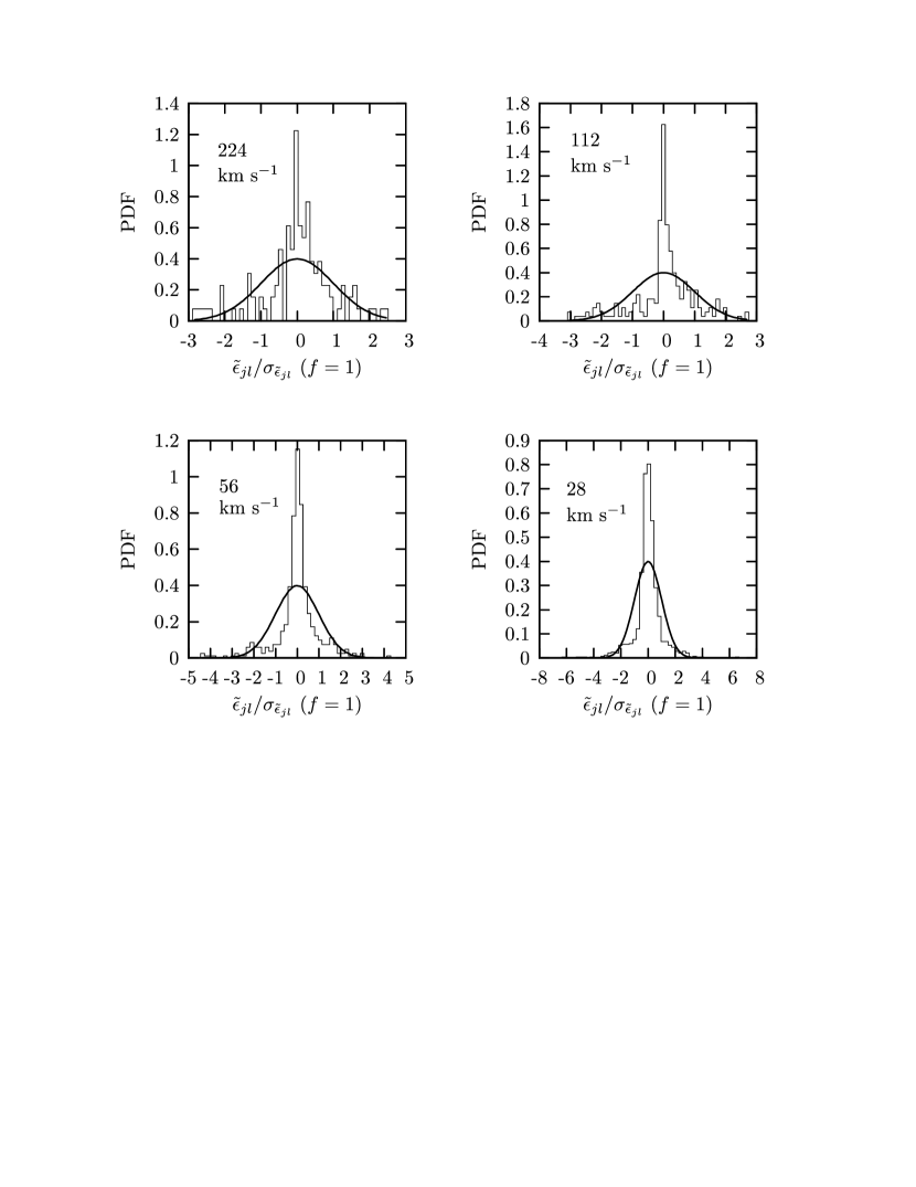
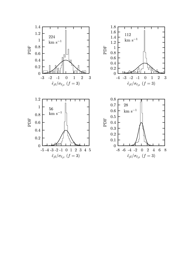
As first step to describe the intermittent behavior of the ${\rm Ly}\alpha$ transmitted flux, we show in Figure 3 the PDFs of the normalized WFCs of flux field $\tilde{\epsilon}^{F}_{jl}/\langle(\tilde{\epsilon}^{F}_{jl})^{2}\rangle^{1/2}$. These distributions are compared with a Gaussian distribution with zero mean and unit standard deviation. On the scales $224$ km s^-1 the PDFs of the normalized WFCs do not strongly deviate from Gaussian fields. But on scales $<$ 224 km s^-1, the central peak and long-tail of the PDFs show that the field is highly non-Gaussian. On the scale 56 km s^-1, the long tail extends to $\tilde{\epsilon}^{F}_{jl}/\langle(\tilde{\epsilon}^{F}_{jl})^{2}\rangle^{1/2}\simeq 5$. That is, the power of some long tail events $(\tilde{\epsilon}^{F}_{jl})^{2}$ can be larger than the mean power $\langle(\tilde{\epsilon}^{F}_{jl})^{2}\rangle$ by a factor of 20-30. This is in agreement with the result based on Keck data (Jamkhedkar et al 2003).

We see that for $f=1,3$ and $5$, the PDFs given by $f=1,3$ and 5 are essentially the same, especially, the central peaks of the PDFs are insensitive to the parameter $f$. This indicates that the statistical result does not depend on data at pixels with low number of $S/N$. This point is important. For instance, a saturated absorption region on scale $j_{s}$ may yield $\tilde{\epsilon}^{F}_{jl}\rightarrow 0$ on smaller scales or $j>j_{s}$, i.e. pixels with a low value of $S/N$. However, we cannot draw information of clustering of cosmic matter from that region. We also can not say whether this region underwent a strong nonlinear evolution. Therefore, the $f$-independence of the PDFs of Figure 3 provides an valuable measurement of the non-Gaussian behavior, irrespective of whether the region is saturated or not.

6.2 Structure functions

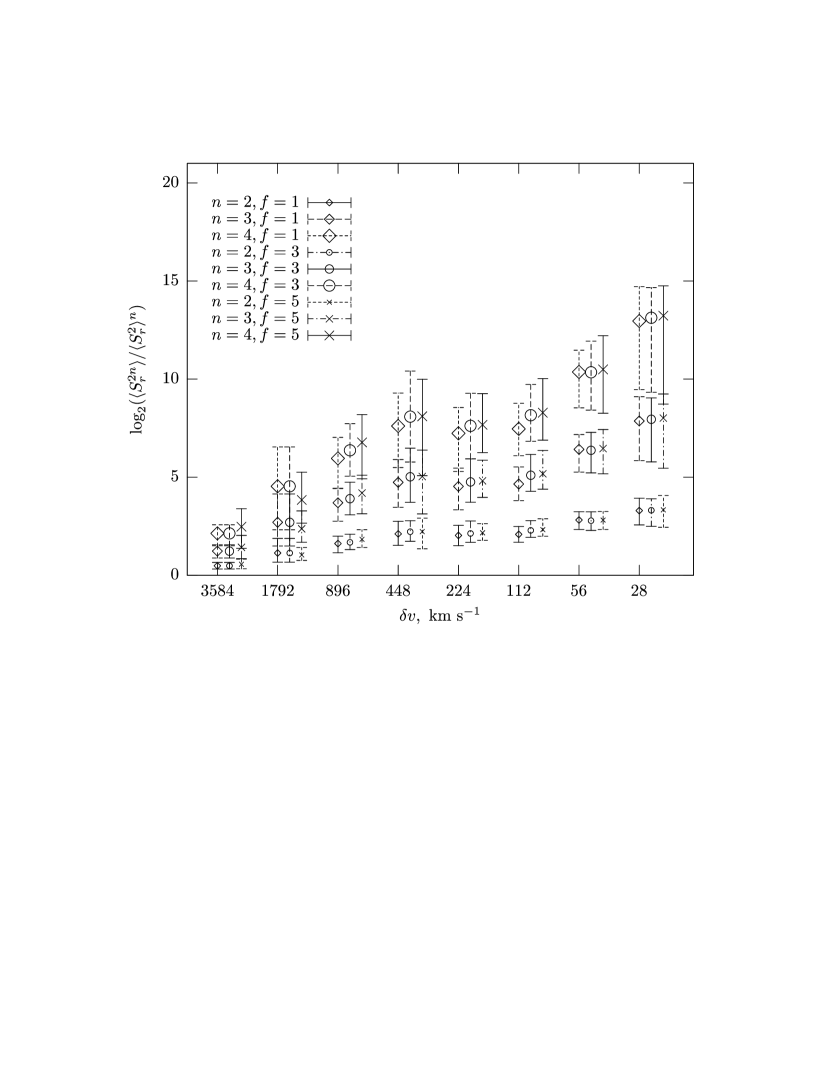
We now calculate the structure functions eqs. (2) or (7) for the transmitted flux fluctuations of HE2347-4342. For real data, the results are illustrated in Figure 4. In calculating the high order moment $S^{2n}_{j}$, we did not subtract the noise term in eq. (14), because as noise is considered Gaussian, its higher order moments are small (see §6.4 below). The error bars are found by bootstrap re-sampling. We see that $\log_{2}[S^{2n}_{j}/(S^{2}_{j})^{n}]$ with $n=2$ has errors even smaller than the power spectrum of Figure 1. This is because the uncertainty in the power spectrum is caused by rare and improbable long tail events in the fluctuations, i.e. the tail of the PDF shown in Figure 3. The large uncertainty of the PDF tail leads to the large uncertainty of the power spectrum. On the other hand, the structure function is the ratio between $S^{2n}_{j}$ and $(S^{2}_{j})^{n}$ and it reduces the effect of individual high spikes (tail events). Therefore, the structure functions are an effective and stable tool for high order statistics. Similar to the power spectra of Figures 1 and 2, and the PDFs of Figure 3, the structure functions of Figure 4 are basically independent of $f$. Therefore, the scale- and $n$-dependencies of the structure function exist regardless of the saturated absorption, and give a measurement of the non-Gaussian clustering of the baryonic gas.

The value of $\log_{2}[S^{2n}_{j}/(S^{2}_{j})^{2}]$ generally is bigger for smaller length scales. For a given $n$, the $j$-dependence of $\log_{2}[S^{2n}_{j}/(S^{2}_{j})^{n}]$ can approximately be fitted by eqs. (2) and (10) with a positive exponent $\zeta$. Therefore, the field of the transmitted flux fluctuations is highly intermittent. This shows again that the cuspy feature of cosmic clustering can be seen in high mass density areas, like massive halos, as well as in low mass density areas, like the clouds of Ly$\alpha$ absorption clouds (He et al. 2004; Pando et al. 2004; He et al. 2005; Kim et al. 2005). Actually the success of the semi-analytical lognormal model (Bi & Davidsen, 1997) in explaining the ${\rm Ly}\alpha$ forest has already indicated that the mass field of the cosmic baryon gas is probably intermittent, because a lognormal field is intermittent.

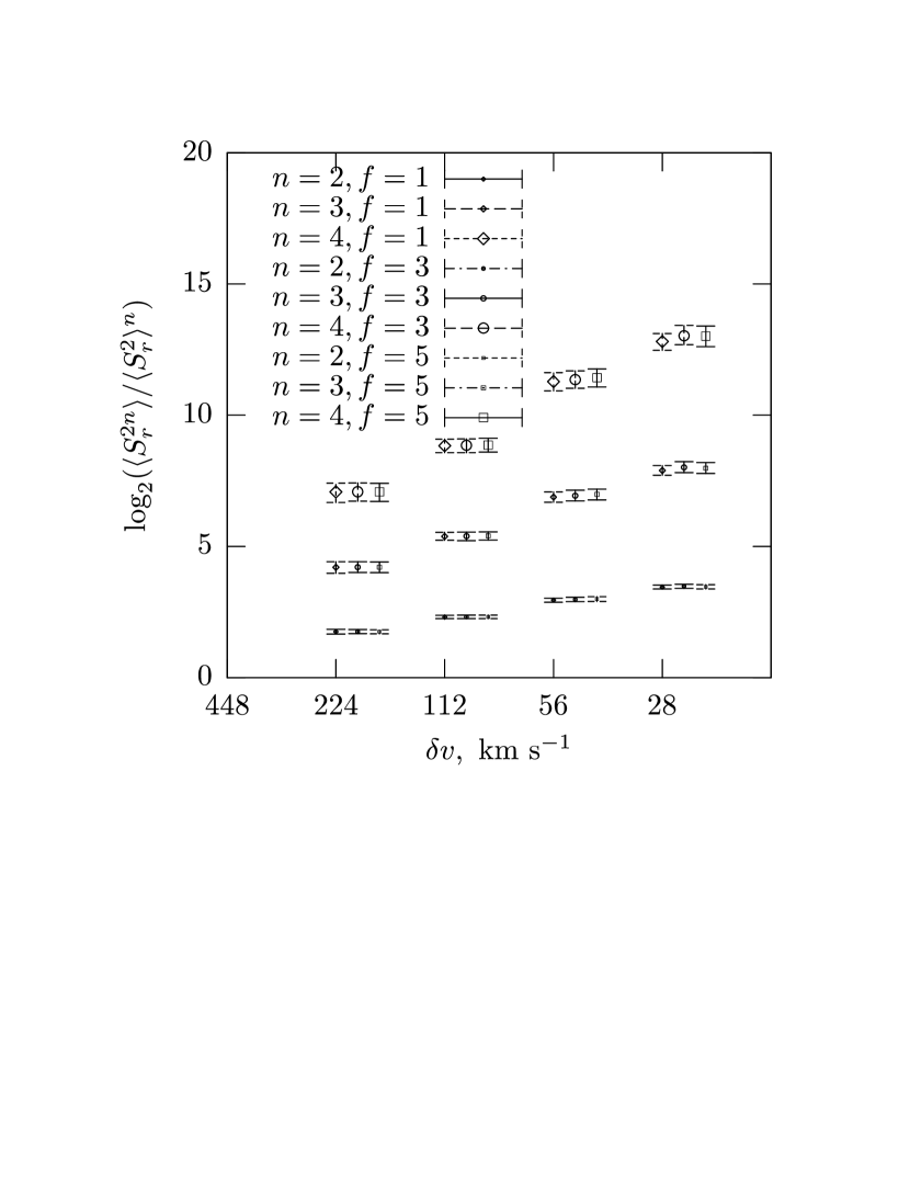
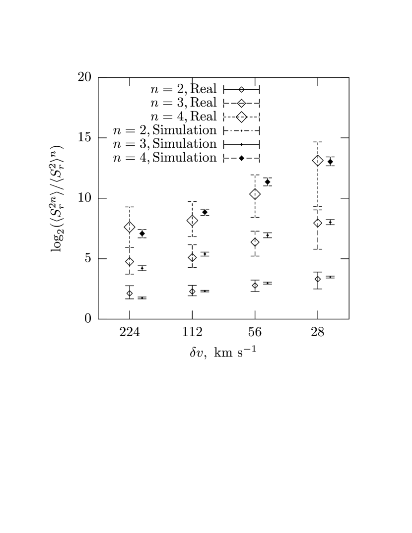
The structure functions measured for the mock samples are shown in Figure 5, in which the error bars are also given by bootstrap re-sampling of the 1000 samples. It shows once again that the statistical uncertainty of the structure function is reliable for a high order statistical test. Figure 5 also shows that the structure function is $f$-independent. Figure 6 gives a comparison between the mock samples and the real data. We see that for all scales from 224 to 28 km s^-1, and all order $n$, the structure functions of the mock samples are consistent with real data within their error bars. The consistence is very good on the smallest scale 28 km s^-1.

6.3 Intermittent exponent

Following the definition of intermittent exponent $\zeta$ eq. (2) or eq. (10), we can calculate $\zeta$ in the scales range $j_{1}$ to $j_{2}$ by

$$\zeta_{n}=-\frac{1}{j_{1}-j_{2}}\log_{2}\left[\frac{S^{2n}_{j_{1}}(S^{2}_{j_{2}})^{n}}{S^{2n}_{j_{2}}(S^{2}_{j_{1}})^{n}}\right].$$ (16)

The result is listed in Table 1. The error of $\zeta_{n}$ is estimated by $\sigma_{\zeta_{n}}=(1/|j_{1}-j_{2}|)\sqrt{{\sigma_{1}^{2}}+{\sigma_{2}^{2}}}$, where $\sigma_{1}$ and $\sigma_{2}$ are the errors of $\log_{2}[{S^{2n}_{j_{1}}}/{(S^{2}_{j_{1}})^{n}}]$, and $\log_{2}[{S^{2n}_{j_{2}}}/{(S^{2}_{j_{2}})^{n}}]$, respectively. The scale $j$ represents a local velocity $\delta v=2^{13-j}\times 3.5~{}$ km s^-1. As expected, Table 1 shows that the values of intermittent exponents of real data and mock samples are consistent with each other on all orders and scales considered.

Table 1: Intermittent exponent

scales $j_{1}$ - $j_{2}$ (${\rm km~{}s^{-1}}$)	$2n$	intermittent exponent $\zeta_{n}$
		real data	mock sample
8 - 9 (112-56)	4	$0.49\pm 0.21$	$0.66\pm 0.03$
8 - 9 (112-56)	6	$1.26\pm 0.48$	$1.54\pm 0.06$
8 - 9 (112-56)	8	$2.18\pm 0.75$	$2.50\pm 0.10$
9 - 10 (56-28)	4	$0.51\pm 0.32$	$0.51\pm 0.03$
9 - 10 (56-28)	6	$1.49\pm 0.76$	$1.08\pm 0.07$
9 - 10 (56-28)	8	$2.6\pm 1.2$	$1.67\pm 0.11$

In Table 2, we list the intermittent exponent of mock samples for different scales ranges. It clearly shows that the intermittent exponent is scale-dependent. We also tried to fit the $j$-dependence of $\log_{2}[S^{2n}_{j}/(S^{2}_{j})^{2}]$ from $j=7$ to 10 by

$$\log_{2}[S^{2n}_{j}/(S^{2}_{j})^{n}]=A+j\zeta_{n}$$ (17)

with assumption of $\zeta_{n}$ to be constant ($j$-independent). We found that the goodness-of-fit, $Q$, (Press et al 1992) of the data to eq.(18) with a constant $\zeta_{n}$ is always $\ll 0.1$. That means that the assumption that $\zeta_{n}$ is independent of scale does not hold. Therefore, $\zeta_{n}$ most likely is scale-dependent. This result is inconsistent with the cuspy center profiles $\rho(r)\propto r^{-\alpha}$ with a constant index $\alpha$, which predicts a constant $\zeta_{n}$ on small scales. Moreover, the $j$-dependence of $\zeta_{n}$ shown in Table 2 is not monotonic. This makes it more difficult to fit with the standard universal profiles. Therefore, the LCDM model seems to predict a different scale-dependence of the intermittent exponent for the Ly$\alpha$ absorption clouds in contrast to the cuspy behavior of the universal profile of dark matter halos.

Table 2: Scale dependence of intermittent exponent

$2n$	$j_{1}-j_{2}$
	7-8	8-9	9-10
4	$0.563\pm 0.028$	$0.66\pm 0.03$	$0.51\pm 0.03$
6	$1.183\pm 0.069$	$1.54\pm 0.06$	$1.08\pm 0.07$
8	$1.77\pm 0.11$	$2.50\pm 0.10$	$1.67\pm 0.11$

6.4 $n$-dependence of structure function

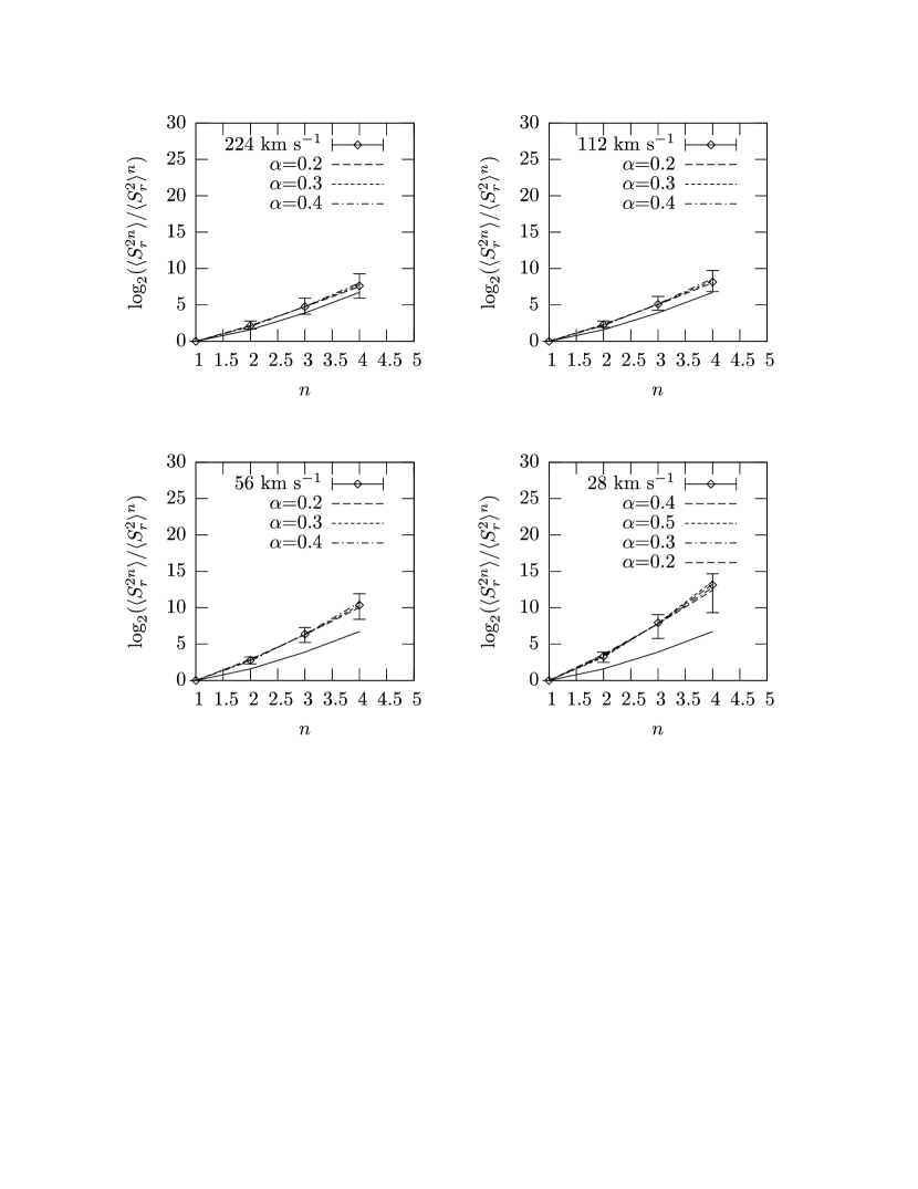
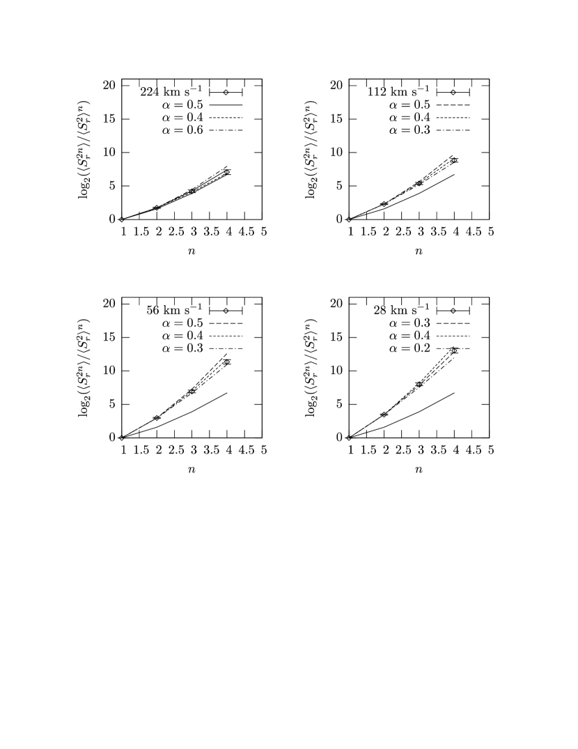
We now turn to the $n$-dependence of the structure functions. Figures 7 and 8 are, respectively, $\log_{2}[S^{2n}_{j}/(S^{2}_{j})^{n}]$ vs. $n$ for the real and mock samples of HE2347-4342 on scales $\delta v=224-28~{}{\rm km~{}s^{-1}}$. For a Gaussian field, the $n$-dependence of $\log_{2}(S^{2n}_{j}/(S^{2}_{j})^{n})$ is given by eq. (3), i.e. $\log_{2}(2n-1)!!$, which is also plotted in Figures 7 and 8. The curves of $\log_{2}[S^{2n}_{j}/(S^{2}_{j})^{n}]$ vs. $n$ for both real and mock samples are much higher than Gaussian field on scales $56~{}{\rm and}~{}28~{}{\rm km~{}s^{-1}}$, but not much different from Gaussian field on scale of 224 km s^-1. Therefore, it is reasonable to ignore the noise term in calculating the high order moment (§6.2).

More interesting is to fit the observed $n$-dependence for $\log_{2}[S^{2n}_{j}/(S^{2}_{j})^{n}]$ with

$$\log_{2}\frac{S^{2n}_{j}}{(S^{2}_{j})^{n}}\propto n^{\alpha}(n-1).$$ (18)

The motivation is to compare the fields with a lognormal field, for which $\alpha=1$. Figure 7 shows that the best fit of $\alpha$ is in the range $\alpha=0.3$ - $0.4$ on scale $56~{}{\rm km~{}s^{-1}}$, and $0.3-0.5$ on $28~{}{\rm km~{}s^{-1}}$. That is, the value of $\alpha$ seems to approach to 1 when scale is small. The transmitted flux field is closer to a lognormal field on small scales. This somewhat supports the lognormal models of ${\rm Ly}\alpha$ forests. Figure 8 shows that values of $\alpha$ given by mock samples always lie in the range from $0.3-0.4$ and are consistent with real data.

7 DISCUSSIONS AND CONCLUSIONS

We have showed that Ly$\alpha$ transmitted flux field of HE2347-4342 is significantly intermittent, especially on small scales. We found that the power spectrum is in good agreement with the data of ${\rm Ly}{\alpha}$ transmitted flux of HE2347-4342. There is no evidence of any discrepancy between the LCDM model from observed intermittent features on scale as small as about $\delta v=28$ km s^-1, and for statistical orders from 2 to 8. Accordingly, there is no need of reducing the power relative to the standard LCDM model up to length scale $0.079$ h^-1 Mpc.

Comparing the current results with our previous studies on the same topic, we found that the intermittency sensitively relies on the quality of both the observed data and simulation sample. In the first stage of our study, we studied the intermittency of Ly${\alpha}$ transmitted flux with Keck data and model samples produced by pseudo-hydro simulations (Pando et al 2002). Although the simulation samples can fit the observed power spectrum, and are also intermittent, the intermittent exponent does not fit the real data. There is a discrepancy between the observed data and simulation sample on small scales. Physically, that is probably because the pseudo-hydro simulations assumed that (1) the baryon distribution is proportional to that of dark matter point-by-point, and (2) the gas temperature is related to the density by a power law equation of state. However, it has been shown that the relation between temperature and IGM density is multi-phased. The relation between temperature and density can approximately be described by a power-law equation. However, for a given density, the temperature actually is not single-valued, but varies from $10^{4}-10^{7}$ K (He et al 2004).

In the second stage, the model samples are produced by full hydro simulations with two assumptions mentioned above (Feng et al 2003). The result was a great improvement with respect to the first round. It shows that the intermittent behavior of the Keck data and simulation is basically consistent with each other, but a discrepancy can still be seen on scale $\delta v=32$ km s^-1. In the current study, the observed data of HE2347-4342 probably is among the best quality for our purpose. Its intermittency is in good agreement with the LCDM model on small scales less than $\delta v=30$ km s^-1.

The star formation and their feedback on the cosmic gas evolution are not considered in our simulation. Generally speaking, there are two types of the feedbacks: (1) photoionization heating by the UV emission of stars and AGNs, and (2) injection of hot gas and energy by stars. The photoionization heating can be properly considered, if the UV background is adjusted by fitting the simulation with the observed mean flux decrement of QSO’s ${\rm Ly}{\alpha}$ absorption spectrum. The effect of injecting hot gas and energy is localized in massive halos, and therefore, its effect is weak when we consider to avoid proximity effects. Therefore, the major conclusions would not be significantly affected even while considering the effect of star formation.

Intermittency is very effective to probe the details of the singular features of a random field. Our simulation samples show that the intermittent exponent of the Ly$\alpha$ transmitted flux field probably is scale-dependent. This result is different from the prediction of universal mass profile with cuspy center $\rho(r)\propto r^{-\alpha}$. If the index $\alpha$ is constant, the intermittent exponent should be scale-independent. Therefore, the scale-dependence of the intermittent exponent indicates that the distribution of baryon gas is decoupled from the underlying dark matter (e.g. He et al 2004, Kim et al 2005). The data of HE2347-4342 only is unable to test the prediction of scale-dependence of the intermittent exponent. More high quality QSO absorption spectra would be very valuable to test the $j$ dependence of $\zeta_{n}$ on small scales.

Figure 1: Power spectrum of the HE2347-4342 transmitted flux for the conditional counting parameter $f=1$ (diamond), 2 (circle), 3. (plus), and 5 (cross).

Figure 2: Power spectra of HE2347-4342 for 1.) real data (circle) and 2.) mock samples (black diamond) by WIGEON simulation with $f=3$. The error bars are the maximum and minimum of bootstrap re-sampling. For clarity, the power spectrum of the simulations is shifted slightly to the right.

Figure 3a: PDFs of $\tilde{\epsilon}^{F}_{jl}/\langle(\tilde{\epsilon}^{F}_{jl})^{2}\rangle^{1/2}$ for the scales $\delta v=224,~{}112,~{}56,~{}28~{}{\rm km~{}s^{-1}}$. Figs. (a),(b) and (c) represent the parameter $f=1,2,~{}{\rm and}~{}3$ respectively. A Gaussian distribution with zero mean and unit standard deviation is also showed in each panel.

Figure 3b:

Figure 3c:

Figure 4: Structure functions $\log_{2}[S^{2n}_{j}/(S^{2}_{j})^{n}]$ vs. scale $\delta v$ (km s^-1) of the data of HE2347-4342. The order $n$ is taken to be $2,3~{}{\rm and}$ 4. The parameter $f$ is taken to be $1,3~{}{\rm and}$ 5. The error bars are given by bootstrap re-sampling. For clarity, the result of $f=$ 3, and 5 are shifted slightly on $X$-axis with respect to $f$=1.

Figure 5: Structure functions $\log_{2}[S^{2n}_{j}/(S^{2}_{j})^{n}]$ vs. scale $\delta v$ (km s^-1) of the mock samples of HE2347-4342. The order $n$ is taken to be 2, 3 and 4. Parameter $f$ is taken to be 1, 3 and 5. The error bars are the maximum and minimum of bootstrap re-sampling. For clarity, the result of $f=3,~{}{\rm and}$ 5 are shifted slightly on $X$-axis with respect to $f=1$.

Figure 6: A comparison between the structure functions of mock samples and real data. The order $n$ is taken to be $2,3~{}{\rm and~{}4}$. The parameter $f$ is equal to 3. The error bars are the maximum and minimum of bootstrap re-sampling for both types of samples.

Figure 7: The $\log_{2}[S^{2n}_{j}/(S^{2}_{j})^{n}]$ vs. $n$ on scales of $\delta v=224,112,56~{}{\rm and}~{}28$ km s^-1 for real data of HE2347-4342. The errors bars are given by the maximum and minimum of bootstrap re-sampling. The fitting curves are $n^{\alpha}(n-1)$. The dotted curves are for Gaussian field, i.e. $\log_{2}[S^{2n}_{j}/(S^{2}_{j})^{n}]=\log_{2}(2n-1)!!$

Figure 8: The same as Figure 8, but for mock samples.