Multi-Dimensional Density Estimation and Phase Space Structure Of Dark Matter Halos

Abstract

We present a method to numerically estimate the densities of a discretely sampled data based on a binary space partitioning tree. We start with a root node containing all the particles and then recursively divide each node into two nodes each containing roughly equal number of particles,until each of the nodes contains only one particle. The volume of such a leaf node provides an estimate of the local density and its shape provides an estimate of the variance. We implement an entropy-based node splitting criterion that results in a significant improvement in the estimation of densities compared to earlier work. The method is completely metric free and can be applied to arbitrary number of dimensions. We use this method to determine the appropriate metric at each point in space and then use kernel based methods for calculating the density. The kernel smoothed estimates were found to be more accurate and have lower dispersion. We apply this method to determine the phase space densities of dark matter halos obtained from cosmological N-body simulations. We find that contrary to earlier studies, the volume distribution function $v(f)$ of phase space density $f$ does not have a constant slope but rather a small hump at high phase space densities. We demonstrate that a model in which a halo is made up by a superposition of Hernquist spheres is not capable in explaining the shape of $v(f)$ vs $f$ relation, whereas a model which takes into account the contribution of the main halo separately roughly reproduces the behavior as seen in simulations. The use of the presented method is not limited to calculation of phase space densities, but can be used as a general-purpose data-mining tool and due to its speed and accuracy it is ideally suited for analysis of large multidimensional data sets.

1 Introduction

One of the basic problems in data mining is to estimate the probability distributions or density distributions based on a discrete set of points (particles) distributed in a multidimensional space. Once the density distribution is known expectation values of other quantities of interest can be derived. Considering the huge amounts of data both astronomy and other fields are facing there is a need for methods that are accurate flexible and fast. However, most of the existing methods encounter problems when applied to higher dimensions. In the particular application of N-body simulations, the estimate of phase space densities is one such problem as it requires an efficient and flexible method for 6 dimensional phase space density estimation for a large variety of equilibrium and non-equilibrium solutions of largely different topology (e.g. highly flattened disks, spheroidal but anisotropic halos, spheroidal nearly isotropic ellipticals).

The simplest method for density estimation is the $k$ nearest neighbor. Consider the radius $r$ enclosing $k$ nearest neighbors then density is given by $k/V_{d}(r)$ where $V_{d}(r)$ is the volume enclosed by a $d$-dimensional sphere of radius $r$ (Loftsgaarden & Quesenberry, 1965). A more accurate method than this is the kernel density estimation (KDE) or popularly known as SPH (Gingold & Monaghan, 1977; Lucy, 1977; Silverman, 1986). The results are sensitive to the choice of kernel function and the bandwidth of the kernel or in other words the number of smoothing neighbors. The later being more important. Variable bandwidth estimators are more superior as compared to the fixed bandwidth estimators. For the multidimensional case simple isotropic bandwidths perform poorly when the data has an anisotropic distribution. In this case one needs to select different bandwidths in different dimensions. In general a co-variance matrix is determined and the bandwidth is selected so as to have constant co-variance in all directions. This leads to anisotropic kernels. The Delaunay tessellation (Okabe et al., 1992; Okabe, 2000; Schaap & van de Weygaert, 2000; Bernardeau & van de Weygaert, 1996) which tessellates space into disjoint regions, performs much better for anisotropic data. Delaunay tessellation is very accurate but also very time consuming.

Most existing methods, including both KDE and Delaunay Tessellation require an a-priori definition of a metric of the n-dimensional space under investigation. A suboptimal choice of metric results in a poor estimate of the density. Metric based density estimators provide optimal approximations, only if co-variance of the data is identical along all dimensions, locally at each point in space. In general, however, data is non-homogeneous and anisotropic. Consequently the above conditions cannot be realized by assuming a global scaling relation among different dimensions. A method is required that is adaptive to the data under investigation. Recently a new method dubbed FiEstAS which is metric free has been proposed by Ascasibar & Binney (2005). FiEstAS is also very fast and efficient. The method relies on a repeated binary decomposition of space (organized by a tree data structure) until each volume element contains exactly one particle. The accuracy of the method depends upon the criteria used for splitting the nodes. In the simplest implementation the dimension to be divided is chosen either randomly or alternately, guaranteeing equal number of divisions for each dimension. The more a particular dimension is tessellated the higher the resolution achieved in that dimension. Ideally we need a scheme which makes more divisions in the dimension along which there is maximum variation and few divisions (or none) along which there is minimum (or no) variation. However, the scheme as described above is data blind and thus fails to optimize the number of divisions to be made in a particular dimension.

In this paper we propose and evaluate a splitting criterion that is based upon the concepts of Information Theory (Shannon, 1948, 1949; MacKay, 2003; Gershenfeld, 1999). Space is tessellated along the dimension having the minimum entropy (Shannon Entropy) or in other words maximum information . Consequently, this scheme optimizes the number of divisions to be made in a particular dimension so as to extract maximum information from the data. This method can also be used to determine the metric that locally gives approximately constant covariance. Kernel based methods can then be used to estimate the densities.

As an application we study the phase space density of dark matter halos obtained from cosmological simulations. The code is available upon request and in future we plan to make it publicly available at the following url
https://sourceforge.net/projects/enbid/

2 Algorithm

The basic problem is to estimate the density function $\rho(\mathbf{x})$ from a finite number $N$ of data points $\mathbf{x^{1},x^{2}..x^{N}}$ drawn from that density function. Here $\mathbf{x^{i}}$ is a vector in a space of $d$ dimensions having components $x^{i}_{1},x^{i}_{2}..x^{i}_{d}$. The overall procedure of our algorithm EnBiD (Entropy Based Binary Decomposition) consists of three steps, which we will describe in detail below. First we tessellate the space into mutually disjoint hypercubes each containing exactly one particle. If $V^{i}$ is the volume of the hypercube containing $i$th particle then its density is $m_{i}/V^{i}$. Second we apply the boundary corrections to take into account the arbitrary shape of the volume containing the data. Third we apply a smoothing technique in order to reduce the noise in the density estimate.

2.1 Tessellation

We start with a root node containing all particles. The node is divided by means of a hyper plane perpendicular to one of the axis into two nodes each containing half the particles. If $j$ is the dimension along which the split is to be performed, the position of the hyper plane is given by the median of $x_{j}$. The process is repeated recursively till each sub-node contains exactly one particle(so-called leaf nodes). Let $V_{i}$ be the volume of the leaf node containing particle $i$, and $m_{i}$ be the particle mass, then the density is given by $\rho_{i}=m_{i}/V_{i}$. An alternative to this, as was originally done in FiEstAS, is to calculate the mean $<x_{j}>$ and then identify two points one on each side which are closest to the mean. The split point is then chosen midway between these two points. $x_{cut}=(x_{left}+x_{right})/2$. This speeds up the tessellation.

In the implementation of FiEstAS the splitting axis alternates between the considered dimensions, which guarantees roughly equal number of divisions per dimension. In the calculation of phase space densities the real and velocity space are known to be Euclidean. Therefore the splitting is done alternately in real and velocity space and in each subspace the axis with highest elongation ($<x_{j}^{2}>-<x_{j}>^{2}$) is chosen to be split. This generates cells that are cubical rather than elongated rectangular in the aforementioned subspace, and also helps alleviate numerical problems that arise when two points have very close values of a particular co-ordinate. We call this decomposition which is implemented in FiEstAS as Cubic Cells while the one free from this as General.

For $N$ particles the binary decomposition results in $2N-1$ nodes out of which there are $N$ leaf nodes each having one particle. The more a particular dimension is tessellated, the more the resolution in that dimension. However, for data that is uniformly distributed in a particular dimension there is actually no need to perform a split in that dimension. This fact can be exploited to increase the accuracy of the results.

For each node we calculate the Shannon entropy $S_{j}$ along each dimension (or subspace) and then select the axis (subspace) with minimum entropy. The dimension having minimum entropy guarantees maximum density variation or clustered structures in that dimension. In other words we split the dimension that has the maximum amount of information. The entropy $S$ along any dimension or subspace is estimated by dividing the dimension or subspace into $N_{b}$ bins of equal size and calculating the number of points $n_{i}$ in each bin (we choose $N_{b}$ to be equal to the number of particles in each node). The probability that a particle is in the $i$th bin is given by $p_{i}=n_{i}/N$ where $N$ is the total number of particles. The entropy is then given by

$$S=-\sum_{i=1}^{n}p_{i}\log(p_{i})$$ (1)

Rather than treating each dimension independently it is also possible to select a subspace (real or velocity space) with minimum entropy and then choose an axis with maximum elongation from this subspace (Cubic Cells). This provides slightly lower dispersion in estimated densities.

2.2 Boundary correction

The data in general might have an irregular shape and may not be distributed throughout the rectangular volume of the root node. Consequently, the densities of particles near the boundary can be underestimated. This is not an issue for systems with periodic boundary conditions but it would be for systems which are for example spherical. In higher dimensions this correction becomes even more important since the fraction of particles that lie near the boundary increases sharply with number of dimensions.

In FiEstAS the following correction is implemented: Suppose a leaf node having a particle at $\mathbf{x^{p}}$ has one of its surfaces in dimension $i$ either $x_{i}=x_{max}$ or $x_{i}=x_{min}$ as a boundary, then the boundary face is redefined such that its distance from the particle is same as the distance of the other face from the particle. For the former the redefinition is $x_{i}=x_{i}^{p}+(x^{p}-x^{min})$ and for the later $x_{i}=x^{p}_{i}-(x^{max}-x^{p}_{i})$. If both the faces lie on the boundary then the scheme fails to apply the correction. Moreover for small sub halos embedded in a bigger halo the sub halos have lower velocity dispersion and occupy a smaller region in velocity space, hence its boundary needs to be corrected even though it is not directly derived from the global boundary. A similar situation also arises near the center of the halos for which the circular velocity $V_{c}(r)\rightarrow 0$ as $r\rightarrow 0$. Moreover in EnBiD we need to calculate the entropy for each node and the boundary effects might decrease the entropy of the system spuriously. Consequently, a boundary correction needs to be applied to each node during the tessellation, and not just to the leaf node at the end of tessellation. In EnBiD for each node having more than a given threshold $n_{b}$ of particles, a node is checked for boundary correction before the calculation of entropy. In a given dimension if $l_{max}$ and $l_{min}$ are the maximum and minimum co-ordinates of a node and $x_{max}$ and $x_{min}$, the corresponding maximum and minimum co-ordinates of the particles inside it, then a boundary correction is applied if simultaneously

$$(l_{max}-x_{max})>f_{b}\frac{x_{max}-x_{min}}{n_{node}-1}$$ (2)

and

$$(x_{min}-l_{min})>f_{b}\frac{x_{max}-x_{min}}{n_{node}-1}$$ (3)

where $f_{b}$ is a constant factor. This is effective in detecting embedded structures. To check for corrections applicable for only one face, the value of $f_{b}$ is chosen to be $5$ times higher. For cubical cells in real and velocity space $f_{b}=0.5N^{1/d}$ was found to give optimal results, where $N$ is the total number of particles in the system. For general decomposition the corresponding value of $f_{b}$ was found to be $2.0N^{1/d}$. The node boundary $l_{max}$ and $l_{min}$ are corrected as

$$l_{max}\rightarrow x_{max}+\frac{x_{max}-x_{min}}{n_{node}-1}$$ (4)

$$l_{min}\rightarrow x_{min}-\frac{x_{max}-x_{min}}{n_{node}-1}$$ (5)

where $(x_{max}-x_{min})/(n_{node}-1)$ is the expected mean inter-particle separation.

The choice of $n_{b}$ is dictated by two factors a) if $d$ is the number of dimensions of the space then a minimum of $d+1$ particles are needed to define a geometry in that space so we set $n_{b}\geq d+1$. If the number of particles in a node are too small this leads to Poisson errors in the calculation of the inter-particle separation so we impose a lower limit of $n_{b}=7$.

2.3 Smoothing

The un-smoothed density estimates have a large dispersion which cannot be reduced even by increasing the number of particles. By smoothing this dispersion can be reduced provided the density does not vary significantly over the smoothing region. We test two different smoothing techniques. The FiEstAS smoothing as proposed by (Ascasibar & Binney, 2005) and the kernel based scheme (KDE).

In FiEstAS smoothing, first the density of each node is calculated assuming that the mass of each particle is distributed uniformly over its leaf node. Next the volume $V_{s}$ centered on that point which encompasses a given smoothing mass $M_{s}$ is calculated. The density estimate is then given by $\rho=M_{s}/V_{s}$. For Cubic tessellation the smoothing cells are also chosen to be exactly cubical in the real and velocity subspaces. To calculate $V_{s}$ an iterative procedure is used. We start with a hyper-box having boundaries in the $i$-th dimension at $x_{i}\pm\Delta_{i}$, $\Delta_{i}$ being the distance to the closest hyper plane along $i$-th axis of the leaf node containing the point $\mathbf{x}$. $\Delta_{i}$ is then doubled until the mass enclosed by smoothing box $M<M_{s}$ and then the interval is halved repeatedly till $|(M-M_{s})/M_{s}|\leq\eta_{tol}$ where $\eta_{tol}$ is a tolerance parameter. Our experiments show that a tolerance parameter of 0.1 gives satisfactory results. Although in FiEstAS the smoothing mass $M_{s}=10m_{p}$ is chosen, we find that choosing $M_{s}=2m_{p}$ gives a higher resolution, while not compromising much on the noise reduction.

In Kernel smoothing a fixed number of nearest neighbors around the point of interest are identified and the density is computed by summing over the contributions of each of the neighbors by using a kernel function. This is known as the adaptive kernel smoothing since the smoothing length is $\propto\rho^{1/d}$, $\rho$ being the density in a $d$ dimensional space. The kernel function can be spherical of the form of $W(u$), $u=\sqrt{\sum_{i=1}^{d}u_{i}^{2}}$ being the distance of the neighbor from the center and $u_{i}$ the corresponding co-ordinates in a $d$ dimensional space, or of the form of $\Pi_{i=1}^{d}W(u_{i})$ known as the product kernel. The standard kernel scheme provides a much poorer estimate of the phase space density, since a global metric is usually unsuitable in accounting for the complex real and velocity structure encountered in many astrophysical systems. However, with a method like EnBiD we can determine the appropriate metric at each point in space and thus force the co-variance to be approximately same along all dimensions. At any given point the correct metric can be calculated by determining the sides of the leaf node which encompasses that point, followed by a coordinate transformation such that the node is transformed into a cube. As we illustrate in the appendix, the kernel density estimator can have a significant bias in the estimated densities. The results we show here are after correcting for this bias. We tested and compared the use of spline and the Epanechnikov kernel function and found the later to be more efficient. For all our analysis we use the Epanechnikov kernel function. Bias correction and other details pertaining to kernel based methods e.g the number of smoothing neighbors are given in the Appendix. The algorithm implemented in EnBiD for nearest neighbor search is based on the algorithm of SMOOTH (Stadel, 1995).

Although the length of the sides of a node provides an accurate estimate of the metric but when trying to smooth over a region, the smoothing region might exceed the boundaries of the actual particle distribution. The smoothing lengths in such case needs to be appropriately redefined. This situation arises in cases where a dimension has very less entropy and has been split many times or near the boundaries of the system where the metric has not been accurately determined. In a given dimension let $l_{max}$ and $l_{min}$ be the maximum and minimum co-ordinates of a smoothing box or a sphere encompassing a fixed number of neighbors $N_{ngb}$ and $x_{max}$ and $x_{min}$ the maximum and minimum co-ordinates of the particles inside it. A smoothing length correction is applied to the box, if simultaneously the distance to both the right and left boundaries given by

$$(l_{max}-x_{max})>25(x_{max}-x_{min})/N_{ngb}$$ (6)

$$(x_{min}-l_{min})>25(x_{max}-x_{min})/N_{ngb}$$ (7)

where $N_{ngb}$ is the number of smoothing neighbors. The metric is redefined with $l_{max}$ and $l_{min}$ set to $x_{max}$ and $x_{min}$. For FiEstAS smoothing also we implement a similar smoothing volume correction. For a given smoothing box of volume $V_{s}$, if $m_{i}$ is the mass contributed by a leaf node to the smoothing box and $v_{i}$ its corresponding volume that falls within the box, then instead of calculating the density as $\rho=\sum m_{i}/V_{s}$, we calculate it as $\rho=(\sum m_{i})/(\sum v_{i})$. This correction is only applied if $(\sum v_{i})/V_{s}<0.5$.

3 Tests

To test the accuracy of the results we generate test data with a given density distribution in a $d$ dimensional space and then perform a comparison with the density estimates given by the code. We employ systems which have an analytical expression of $6$ dimensional phase space density $f$, namely an isotropic Hernquist sphere (c.f. Ascasibar & Binney (2005)) and an isotropic halo with a Maxwellian velocity distribution (c.f. Arad et al. (2004) ). The test cases are generated by discrete random sampling of this density function $f$ using a fixed number of particles $N$. We show here results of tests done in 6 dimensions only and with boundary correction and smoothing. Results pertaining to $3$ dimensions and effects of boundary correction and smoothing are discussed in detail in Ascasibar & Binney (2005).

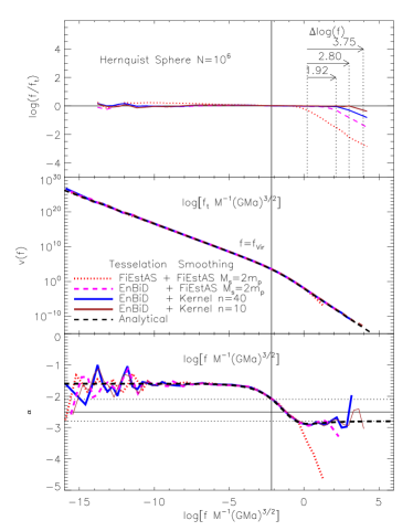
Figure 1: Dependence of fraction $f/f_{t}$ on $f_{t}$ and $v(f)$ and $\alpha(f)$ on $f$ for a Hernquist sphere with $N=10^{6}$ particles obtained by different algorithms for density estimation. Vertical dotted lines mark the position where $f/f_{t}=0.5$. EnBiD resolves the high-density regions better by about $2$ decades in density. Kernel Smoothing using the metric as determined by EnBiD performs even better (a gain in resolution of about 3-4 decades). Using a smaller number of smoothing neighbors results in higher resolution.

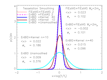
Figure 2: Probability distribution$P(\log(f/f_{t}))$ for a Hernquist sphere with $N=10^{6}$ particles obtained by different algorithms for density estimation.

3.1 Hernquist Sphere

For a Hernquist (1990) sphere of total mass $M$ and scale length $a$ the real space density is given by

$$\rho(r) = \frac{M/(2\pi a^{3})}{(r/a)(1+r/a)^{3}}$$

and gravitational potential is given by

$$\phi(r)=-\frac{GM}{a}\frac{1}{1+r/a}.$$

The phase space density as a function of energy $E=v^{2}/2+\phi(r)$ is

$$f(E) = \frac{M/a^{3}}{4\pi^{3}(2GM/a)^{3/2}}\times$$ (9)

$$\frac{3\sin^{-1}q+q\sqrt{1-q^{2}}(1-2q^{2})(8q^{4}-8q^{2}-3)}{(1-q^{2})^{5/2}}\ \ \ \ \ \ \ \$$

where

$$q=\sqrt{-\frac{E}{GM/a}}.$$

First we generate a random realization in real space corresponding to density given by Eq. (3.1). Then we use von Neumann rejection technique to generate the velocities that sample the distribution Press et al. (1992).

$$p(v)dv=\frac{4\pi}{\rho(r)}f(v^{2}/2+\Phi(r))v^{2}dv$$

Further details can be found in Ascasibar & Binney (2005). For calculating the virial quantities of a Hernquist sphere we use $c=R_{Vir}/a=4.0$ which roughly corresponds to an $NFW$ halo with $c=8.0$.

In top panel of Fig. 1 we plot the ratio of numerically estimated phase density $f$ evaluated by the respective method to the analytical phase space density $f_{t}$ , as a function of $f_{t}$ for a Hernquist sphere sampled with $10^{6}$ particles. $f$ is calculated by binning the particles in $80$ logarithmically spaced bins in $f_{t}$ with at least $5$ particles per bin and then evaluating the mean value of the estimated density of all the particles in the bin.

Ideally one expects the plot to be a straight line with $f/f_{t}=1$. It can be seen from the figure that the density is well reproduced for most of the halo for about $18$ decades in density except near the very center where the density is very high. Both FiEstAS and EnBiD tessellation, followed by FiEstAS smoothing with $M_{s}=2m_{p}$, underestimate the density in the region of very high density, however when compared to FiEstAS tessellation the high density cusp is resolved better by EnBiD by about 2 decades in density. In real space there is more variation of density as compared to velocity space. EnBiD accounts for this by allocating more divisions in real space thereby achieving higher spatial resolution, whereas FiEstAS gives equal weight to both spaces and ends up thus compromising the spatial resolution. When kernel smoothing is employed along with metric as determined by EnBiD tessellation (EnBiD+Kernel Smooth), there is a further gain in resolution by about $3$ and $4$ decades for smoothing neighbors $n=40$ and $n=10$ respectively. Lowering the number of smoothing neighbors results in higher resolution.

Next we compare the volume distribution function $v(f)$ as reproduced by the code. Numerically $v(f)$ is evaluated by binning the particles as before in logarithmically spaced bins of $f$. If $m_{bin}$ is the mass of all the particles in the $i$ th bin, the density of the bin being $f_{bin}=(f_{i+1}+f_{i})/2$ then $v(f_{bin})=(m_{bin}/f_{bin})/(f_{i+1}-f_{i})$. Statistical error in each bin is given by $\Delta f=f_{bin}-<f_{bin}>$ (where $<f_{bin}>$ is the mean value of density of all the particles in the bin). Analytically the volume distribution function is given by

$$v[f(E)]=\frac{g(E)}{f^{\prime}(E)}$$ (10)

where $g(E)$ is the density of states. For a Hernquist sphere

$$g(E) = \frac{2\pi^{2}a^{3}(2GM/a)^{1/2}}{3q^{5}}[3(8q^{4}-4q^{2}+1)cos^{-1}q$$

$$-q(1-q^{2})^{1/2}(4q^{2}-1)(2q^{2}+3)]$$

It can be seen from middle panel of Fig. 1 that $v(f)$ is well reproduced by both FiEstAS and EnBiD. However, in the high density region FiEstAS underestimates $v(f)$ which results in steepening of the volume distribution function at the high $f$ end, while EnBiD estimates the $v(f)$ accurately to much higher densities.

This can be seen more clearly in lower panel of Fig. 1 where we plot the logarithmic slope denoted by $\alpha$ of the volume distribution function as function of density $f$.

$$\alpha=\frac{d\log(v(f))}{d\log(f)}$$

FiEstAS can reproduce the slope parameter $\alpha$ only till $f/f_{Vir}=10^{2}$ whereas EnBiD can reproduce it till $f/f_{Vir}=10^{4}$ and EnBiD+Kernel Smooth can reproduce it till $f/f_{Vir}=10^{5}$ and $f/f_{Vir}=10^{6}$, for smoothing neighbors $n=40$ and $10$ respectively.

In order to get an estimate of the dispersion in the reproduced values of $f$ and in order to check the effectiveness of smoothing we plot in Fig. 2 the probability distribution of $f/f_{t}$. The distribution can be fitted with a log-normal distribution and the fit parameters are also shown in the figure. The bias is less than $0.03$ dex for all the methods.The un-smoothed estimates have a dispersion of $0.37$ dex. FiEstAS smoothing with $M_{s}=2$ is equivalent to Kernel smoothing with smoothing neighbors $n=40$. Both of them have a dispersion of about $0.1$ dex. For kernel smoothing lowering the smoothing neighbors to $n=10$ results in an increase in dispersion to $0.18$ dex.

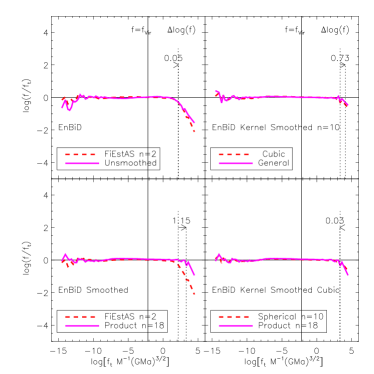
Figure 3: Dependence of fraction $f/f_{t}$ on $f_{t}$ for a Hernquist sphere with $N=10^{6}$ particles obtained by different algorithms for density estimation.

The EnBiD tessellation in the results as analyzed above was done with Cubic Cells in real and velocity space. In top right panel of Fig. 3 we compare the results as obtained with General decomposition where each dimension is treated independently. Kernel smoothing with smoothing neighbors $n=10$ was employed for both of them. The estimates are nearly identical. There is a slight gain in resolution but the estimates with General decomposition were also found to have a slightly higher dispersion in the estimates. In bottom right panel we compare the result of smoothing between a product kernel and a spherical kernel. There is very little difference between the estimates. The number of neighbors were chosen so as to have identical dispersions in both the estimates. When using the kernel in product form about double the number of neighbors are needed to obtain identical dispersion.

In top left panel we compare the un-smoothed densities with FiEstAS smoothed densities. For both of them EnBiD scheme is used for tessellation. The un-smoothed estimates are the densities as determined from the volume of the leaf nodes generated by the tessellation procedure. The FiEstAS smoothing only reduces the dispersion the resolution remains nearly unaltered. The resolution and accuracy is essentially determined by the density of the leaf nodes. Next we compare the FiEstAS smoothing with cloud in cell scheme (Hockney & Eastwood, 1981) of density estimation. The cloud in cell (CIC) method of density estimation is a special case of smoothing with a product kernel along with a linear kernel function $W(u)\propto(1-u)$. Although the FiEstAS smoothing is similar to the cloud in a cell scheme of density estimation but is still unique in its own respect. The main difference being that the clouds which are the leaf nodes in case of FiEstAS smoothing are disjoint whereas in cloud in cell scheme or in general for Kernel based schemes they are overlapping. They can smooth over much smaller regions and hence achieve higher resolution as compared to FiEstAS smoothing. In bottom left panel we plot the estimates of FiEstAS smoothing alongside the estimates as obtained with product kernel with smoothing neighbors n=18. Instead of a linear kernel function we use the Epanechnikov kernel. It can be seen from the figure that the resolution achieved with product kernel is higher as compared to that of FiEstAS smoothing.

When decomposition was done alternately in each dimension the median criterion gave more accurate results. However for EnBiD decomposition choosing the splitting point at either the mean or the median both gave similar results for density estimation of a hernquist sphere, but for a system having substructures the mean criterion gave better results. For all our analysis unless otherwise mentioned, for evaluating phase space densities we use EnBiD decomposition with Cubic Cells to determine the metric and then use the method of spherical kernel smoothing for calculating densities. The mean criterion is used for choosing the splitting point. The number of smoothing neighbors $n$ is chosen to be $40$, although choosing $n=10$ gives higher resolution but it also has higher dispersion which means that the volume distribution function will be smoothed out below the scale set by the dispersion (see §3.2 for more explanation).

Table 1: Comparison of time needed to calculate densities by various methods: This is the time taken to calculate the six dimensional phase space density of a Hernquist sphere with $10^{6}$ particles on an AMD XP2000+ processor having a clock speed of 1666.67 MHz

Method		Tree	Smooth	Total
Tessellation	Smoothing	Building
AD Delaunay				$1week$
AB FiEstAS	FiEstAS $M_{s}=10m_{p}$	$4$s	$730$s	$724$s
FiEstAS	FiEstAS $M_{s}=10m_{p}$	$8$s	$522$s	$532$s
FiEstAS	FiEstAS $M_{s}=2m_{p}$	$8$s	$306$s	$317$s
EnBiD	FiEstAS $M_{s}=2m_{p}$	$19$s	$336$s	$356$s
EnBiD	Kernel $N_{sm}=40$	$19$s	$843$s	$863$s
EnBiD	Kernel $N_{sm}=10$	$19$s	$405$s	$426$s

In Table. 1 we compare the CPU time needed to estimate the phase space density of $10^{6}$ particles in a Hernquist sphere by various methods and techniques. The time as reported by Ascasibar & Binney (2005) for FiEstAS is labeled as AB FiEstAS and the time as reported by Arad et al. (2004) for Delaunay Tessellation method as AD Delaunay. It can be seen that most of the time is needed for smoothing. For both FiEstAS and Kernel smoothing, increasing the smoothing mass or the number of smoothing neighbors, increases the time. Our implementation of FiEstAS smoothing is slightly faster as compared to that of Ascasibar & Binney (2005) due to better cache utilization. This is achieved by ordering the particles just as they are arranged in the binary tree. The kernel smoothing which gives more accurate results requires a modest $20\%$ more time as compared to the time reported in Ascasibar & Binney (2005) for FiEstAS. For median splitting it is possible to speed up the neighbor search by about $10\%$.

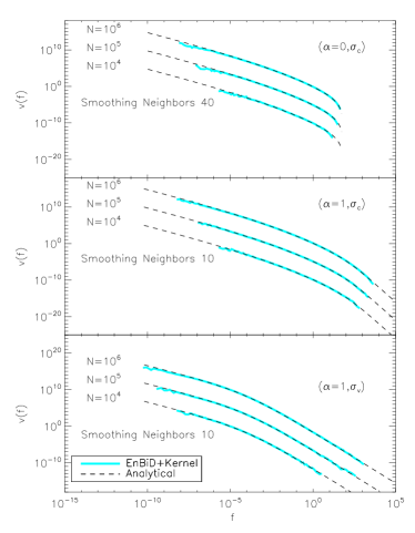
Figure 4: The cumulative distribution of $f/f_{t}$ as measured in different bins of $f_{t}$ for three different mock systems. The density is progressively overestimated in low density regions.

3.2 Maxwellian Velocity Distribution Models

For these models the phase space density is given by

$$f(r,v) = \rho(r)[2\pi\sigma(r)^{2}]^{-3/2}e^{v^{2}/2\sigma(r)^{2}}$$ (11)

where $\rho(r)$ is the real space density given by

$$\rho(r) = \frac{e^{-r/(5r_{s})}}{(r/r_{s})^{\alpha}(1+r/r_{s})^{3-\alpha}}$$

The velocity dispersion is assumed to be either constant with $\sigma_{c}(r)=0.1$ or variable with $\sigma_{v}(r)=\sqrt{M(r)/r}$. We generate models with $\alpha=0$ and $\alpha=1$.

The volume distribution function $v(f)$ for such systems is given by

$$v(f) = \frac{(4\pi)^{2}}{f}\int_{0}^{r(f)}r^{2}\sigma(r)^{3}\sqrt{2\log\frac{f(r)}{f}}dr$$ (12)

where

$$f(r)=\frac{\rho(r)}{[2\pi\sigma(r)^{2}]^{3/2}}$$ (13)

In Fig. 4 we show the volume distribution function as recovered by EnBiD along with kernel smoothing for three different models 1) $\alpha=0,\sigma_{c}$ 2) $\alpha=1,\sigma_{c}$ and 3) $\alpha=1,\sigma_{v}$ and with three different particle resolutions $N=10^{4}$ , $N=10^{5}$ and $N=10^{6}$. For the highest resolution the volume distribution can be recovered for about $9$ to $13$ decades in $f$. The range of densities over which the $v(f)$ is reliably recovered increases with increasing particle number. For systems with a sharp transition in slope of $v(f)$ for example $\alpha=0,\sigma_{c}$ system, Delaunay Tessellation was found to significantly over-estimate $v(f)$ (Fig-A2 Arad et al. (2004)), because the measured $v(f)$ can be thought of as a convolution of the exact $v_{t}(f)$ with a fixed window function $p(f/f_{t})$. The narrower the $p(f/f_{t})$ the closer is $v(f)$ to $v_{t}(f)$. If $v_{t}(f)$ varies significantly over scales smaller than the width of $p(f/f_{t})$ the shape of recovered $v(f)$ will be affected. The $v(f)$ will be over-estimated for a system with a sharp change in the slope of $v(f)$. Moreover due to the width of $p(f/f_{t})$ the effective cut-off value of $f$ is also higher as compared to the theoretically expected upper bound. A bias in $p(f/f_{t})$ will also affect the results. Delaunay Tessellation estimates have a width of about one decade in the distribution of $p(f/f_{t})$. With EnBiD (using smoothing neighbors $n=40$) for $\alpha=0,\sigma_{c}$ system at the high $f$ end there is very little width in the recovered values of $f$, this is the reason that $v(f)$ is recovered better by EnBiD as compared to Delaunay Tessellation (Fig. 4). For other systems the range of $f$ over which $v(f)$ is recovered is slightly higher for EnBiD (using smoothing neighbors $n=10$) as compared to Delaunay Tessellation (Fig-A2 and A3 Arad et al. (2004)).

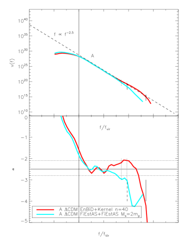
Figure 5: Comparison between density estimators EnBiD and FiEstAS in extracting the volume distribution function and the slope parameter $\alpha$ of a $\Lambda$CDM halo. The vertical dotted lines mark the position of $f=f_{discr}$ and $f=f_{relax}$ ($f_{discr}$ being less than $f_{relax}$). The solid vertical line marks the point where statistical errors ( $\Delta f/f>0.1$ in a bin) in calculation of $v(f)$ become important (dashed one for FiEstAS) . The estimator FiEstAS fails to resolve the high density regions accurately and this results in steepening of the $v(f)$ profile.

4 Phase Space Structure of Dark Matter Halos

We are now applying our tools to the phase space structure of virialized dark matter halos in a concordance $\Lambda$CDM universe (Spergel et al., 2003; Melchiorri, Bode, Bahcall, & Silk, 2003). The structure of these halos in real space has been studied in great detail over the past decade and the radial density profile is known to follow an almost universal form known as the NFW (Navarro, Frenk, & White, 1996, 1997) profile (see however Navarro et al. (2004) for a new $\alpha$ profile).

$$\rho(r)=\frac{\rho_{s}}{(r/r_{s})(1+r/r_{s})^{2}}$$ (14)

The dark matter particles are collisionless and obey the collisionless Boltzmann equations. For a collisionless spherical system in equilibrium with a given density profile $\rho(r)$ the phase space density $f(r,v)$ can be calculated using the Eddington equation (Binney & Tremaine, 1987).

$$f(\varepsilon) = \frac{1}{\sqrt{8}\pi^{2}}\left[\int_{0}^{\varepsilon}\frac{d^{2}\rho}{d\psi^{2}}\frac{d\psi}{\sqrt{\varepsilon-\psi}}-\frac{1}{\varepsilon}\left(\frac{d\rho}{d\psi}\right)_{\psi=0}\right]$$

Since $f$ is a function of six variables it is hard to study except in cases where there are isolated integrals of motion which reduce the number of independent variables. To study the structure of phase space density, the function $v(f)$ is introduced which is the volume distribution function of $f$. $v(f)df$ is the volume of phase space occupied by phase space elements having density between $f$ to $f+df$. Arad et al. (2004) calculated the phase space density using Delaunay Tessellation in 6 dimensions and studied the volume distribution function of halos obtained from simulations. They found that $v(f)$ follows an almost universal form which is a power law with slope $-2.5\pm 0.05$ which is valid for about four decades from $f_{Vir}$ to $f_{Vir}10^{4}$. $f_{Vir}$ is an estimate of the phase space density in the outer parts of the halo.

$$f_{Vir} = \frac{\bar{\rho_{Vir}}}{\pi^{3/2}V_{Vir}^{3}}$$

$$= \left[\frac{3\Delta\rho_{c}}{4\pi^{4}G^{3}}\right]^{1/2}\frac{1}{M_{Vir}}$$

$$= \frac{1.64\times 10^{9}h^{2}\>{\rm M_{\odot}}\>{\rm kpc}^{-3}(\>{\rm km}\,{\rm s}^{-1})^{-3}}{(M_{Vir}/\>{\rm M_{\odot}}h^{-1})}\ \ \ \ \ \textrm{ Using $\Delta=101$}$$

This behavior was also found to be independent of redshift and the mass of the halo. Ascasibar & Binney (2005) used the FiEstAS algorithm to calculate the phase space densities and confirmed the above result and in addition found slight deviations both at low and high $f$ end. At the low $f$ end (near $f_{Vir}$) the slope was found to be flatter than $-2.5$ and at the high $f$ end it was found to be significantly steeper. At the high $f$ end there are two relevant numerical phase space densities, above which two-body relaxation and discreteness effects in simulations start dominating. The phase space density above which the two body relaxation is shorter than the age of the universe is given by (Diemand et al., 2004)

$$f_{relax} = \frac{0.34}{(2\pi)^{3/2}G^{2}\ln\Lambda}\frac{1}{m_{p}t_{0}}$$ (15)

$$= \frac{1.94\times 10^{7}h^{2}\>{\rm M_{\odot}}\>{\rm kpc}^{-3}(\>{\rm km}\,{\rm s}^{-1})^{-3}}{(m_{p}/\>{\rm M_{\odot}}h^{-1})}$$ (16)

The above value is obtained by assuming a Coulomb logarithm of $\ln\Lambda=6$ and using $t_{0}=14.5Gyr$ as the age of the Universe. The phase space density, above which the discreteness effects discussed by Binney (2004) become important, is

$$f_{discr} = \frac{(\Omega_{m}\rho_{c})^{2}}{H_{0}^{3}m_{p}}$$ (17)

$$= \frac{6.93\times 10^{6}h^{2}\>{\rm M_{\odot}}\>{\rm kpc}^{-3}(\>{\rm km}\,{\rm s}^{-1})^{-3}}{(m_{p}/\>{\rm M_{\odot}}h^{-1})}$$ (18)

Since the steepening was found to roughly coincide with these densities, this effect was attributed by Ascasibar & Binney (2005) to the numerical effects of the simulations.

We analyze $5$ halos at $z=0$ simulated in a $\Lambda$CDM cosmology with $\Omega_{\lambda}=0.7$, $\Omega_{m}=0.3$. To evaluate the phase space densities we use the EnBiD scheme along with kernel smoothing employing $n=40$ neighbors. Halos A, B, and C were isolated from a cosmological simulation of $128^{3}$ dark matter particles in a $32.5h^{-1}\>{\rm Mpc}$ cube performed by $AP^{3}M$ code (Couchman, 1991) and were then re-simulated at higher resolution from $z=50$ to $z=0$ using the code GADGET (Springel, Yoshida, & White, 2001). Halo A’ is a warm dark matter (WDM) realization of halo A which was generated by suppressing power on scales smaller than the size of the halo. Halo D is from a simulation done with an ART code (Kravtsov et al., 1997) with a box size of $80h^{-1}\>{\rm Mpc}$. Further details are given in Table. 2. For calculating phase space densities we use the EnBiD tessellation scheme and smoothing is done with a spherical kernel employing $n=40$ neighbors.

Table 2: Properties of halos whose phase space structure is analyzed here: $N_{cut}$ is the number of particles that lie within a cutoff radius $R_{cut}$. These are the particles that are used for calculating the volume distribution function $v(f)$ of the halo.

Halo	$N_{\mathrm{cut}}$	$R_{\mathrm{cut}}$	$R_{Vir}$	$M_{Vir}$	Hubble $h$	Softening	Code	Power
					Parameter			Spectrum
		$\>{\rm kpc}$	$\>{\rm kpc}$	$\>{\rm M_{\odot}}$		$\>{\rm kpc}$
$A$	$6.2\times 10^{5}$	$348.9$	$348.9$	$2.11\times 10^{12}$	$0.65$	$0.30$	GADGET	$\Lambda$CDM
$B$	$6.1\times 10^{5}$	$692.6$	$692.6$	$1.65\times 10^{13}$	$0.65$	$1.53$	GADGET	$\Lambda$CDM
$C$	$3.2\times 10^{5}$	$463.2$	$463.2$	$4.93\times 10^{12}$	$0.65$	$1.53$	GADGET	$\Lambda$CDM
$D$	$6.5\times 10^{6}$	$1854.0$	$1854.0$	$3.2\times 10^{14}$	$0.70$		ART	$\Lambda$CDM
$A^{\prime}$	$4.5\times 10^{5}$	$312.1$	$312.1$	$1.51\times 10^{12}$	$0.65$	$0.30$	GADGET	$WDM$

It can be seen from Fig. 5 that at the high $f$ end there are differences between the phase space properties of halos as reproduced by EnBiD (kernel smoothing using $40$ neighbors) and FiEstAS (FiEstAS smoothing using smoothing mass $M_{s}=2m_{p}$). We argue that the steepening of the volume distribution function as found by Ascasibar & Binney (2005) is probably an artifact of the FiEstAS algorithm since such a steepening also appears in tests done with a pure Hernquist sphere (§3.1). For EnBiD we do not see such steepening; on the contrary, we see a slight hump. This however does not preclude the association of discreteness and relaxation effects with the phase space structure of halos. Since we do not know the real phase space density of the halo it is difficult to disentangle any such effect from the effect of the estimator. For a WDM halo whose profile we expect to be the same as that of a Hernquist sphere we do see a sudden change in slope at around $f_{relax}$ (Fig. 10). Also the slope parameter of $\Lambda$CDM halos have a maximum which is around $f_{discr}$ and beyond this it starts to fall off Fig. 8. At the low $f$ end the flatness in $v(f)$ profile is partly due to the truncation of the halo at a finite radius $r=R_{Vir}$. This is demonstrated in Fig. 6 where for a synthetic Hernquist sphere with $R_{cut}=R_{Vir}$ the $v(f)$ profile is found to flatten out beyond $f=f_{Vir}$ and $\alpha(f)$ rises sharply. The cosmological halos exhibit a flattening that is more pronounced than the synthetic halos. This suggests that their structure is slightly different from that of an equilibrium spherical model corresponding to a given density profile. Models with anisotropy in the velocity dispersion also do not seem to suggest any extra flattening of the $v(f)$ profile. One possibility which was suggested earlier (Ascasibar & Binney, 2005) was that this could be due to depletion of low density phase space by the presence of high density sub halos co-occupying the same space. This can be ruled out as the low $f$ behavior of a WDM halo that does not exhibit significant substructure is identical to that of a $\Lambda$CDM halo.

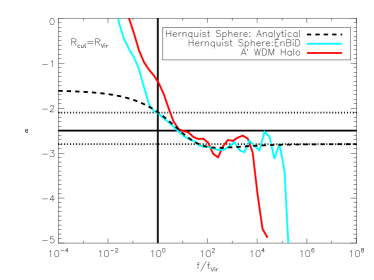
Figure 6: Effect of truncation on the slope parameter $\alpha$ as extracted from a mock Hernquist sphere. The dotted line is the true analytical profile of a Hernquist sphere. For a halo whose $R_{cut}=R_{Vir}$ and $c=4.0$ the $\alpha$ profile can only be extracted till $f=f_{Vir}$. The rise in value of $\alpha$ beyond this is due to truncation of the halo. The thin dark line is for a WDM halo obtained from simulations.

Next we analyze the phase space structure of halos simulated in a $\Lambda$CDM cosmology. We see the existence of a slight departure from the constant power law behavior at the high $f$ end (Fig. 7). The slope parameter $\alpha$ (Fig. 8) has a minimum at around $f/f_{Vir}=10$ and then it rises reaching a peak at around $f/f_{Vir}=10^{4}$. Beyond this it starts to falls off.

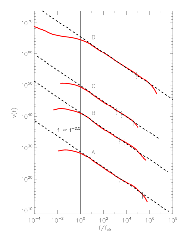
Figure 7: Volume distribution function of phase space density, $v(f)$ for four halos obtained from $\Lambda$CDM simulations. The values of $v(f)$ for halos B,C and D have been shifted by 10,20 and 30 decades respectively for the sake of clarity. For reference $v(f)\propto f^{-2.5}$ curve (matched at $f/f_{Vir}=10$ )is plotted by a dotted line. An explanation of vertical lines is given in Fig. 5.

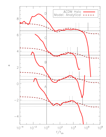
Figure 8: The dependence of slope parameter $\alpha$ on $f$ for four halos obtained from $\Lambda$CDM simulations. The values of $\alpha$ for halos B,C and D have been shifted by 3,6 and 9 respectively for the sake of clarity. An explanation of vertical lines is given in Fig. 5. The dashed line represents the analytical profile of the parent $+$ substructure model. The dotted line is the profile as estimated by EnBiD for the synthetic realization of the corresponding model. The parameter $\alpha$ does not have a constant value of $-2.5$ but has a dip and rise and is bounded between $-2.8$ (the asymptotic value of a Hernquist sphere) and $-2.1$ (the value predicted by the AD Toy model) which are indicated by horizontal dotted lines.

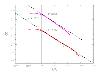
Figure 9: The volume distribution function of phase space density $v(f)$ for a $\Lambda$CDM and a WDM halo. The WDM profile has been shifted vertically by 10 decades. An explanation of vertical lines is given in Fig. 5. The WDM profile is significantly steeper in high density regions as compared to $v(f)\propto f^{-2.5}$ behavior which is indicated by a dashed line.

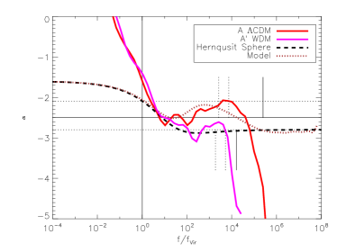
Figure 10: The dependence of slope parameter $\alpha$ on $f$ for a $\Lambda$CDM and a WDM halo. The behavior of WDM halo profile is in agreement with that of a Hernquist Sphere while that of $\Lambda$CDM halo is close to that of a parent $+$ substructure model. The vertical lines mark the position of $f_{stat},f_{relax}$ and $f_{discr}$ for the $\Lambda$CDM halo.

In order to check whether the power law type behavior of the volume distribution function is due to the substructure or whether it is associated with the virialization process we simulated a WDM halo whose power on small scales has been suppressed and we find that it has a steeper slope at the high $f$ end (Fig. 9). Its slope parameter $\alpha$ as a function of $f$ is roughly consistent with that of a Hernquist sphere (Fig. 10). This suggests that the shape of the volume distribution function is governed by the amount of substructure and its mass function.

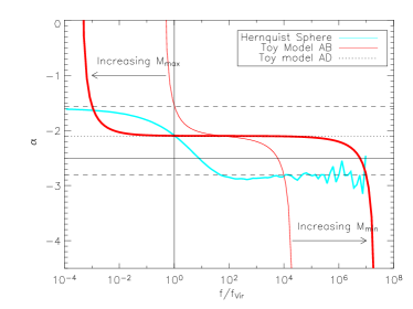
Figure 11: Dependence of slope parameter $\alpha$ on $f$ as predicted by the toy model proposed in Arad et al. (2004) (AD) and the subsequent modification suggested by Ascasibar & Binney (2005) (AB). In the limit the parameter $m_{min}\rightarrow 0$ and parameter $m_{max}\rightarrow\infty$ the AB model goes over to AD model.

4.1 A Toy Model:Superposition of Sub Halos

An elegant toy model to explain the near power law behavior of the volume distribution function of simulated $\Lambda$CDM halos was proposed by Arad et al. (2004) (model AD) In this model the halo is assumed to be made up of a superposition of sub halos with a given mass function of $dn/dm\propto m^{-\gamma}$ each obeying a universal functional form for $f$. The volume distribution function can then be written as

$$v(f)=\int_{0}^{\mu M}\frac{dn}{dm}v_{m}(f)dm\propto f^{-(4-\gamma)}$$ (19)

where $\mu M$ is the mass of the largest sub halo. However, for $\gamma=1.9$, as derived by (De Lucia et al., 2004), this model predicts $v(f)\propto f^{-2.1}$, rather than $v(f)\propto f^{-2.5}$ as found in Arad et al. (2004). Ascasibar & Binney (2005) modified this model by pointing out that the lower limit of the integral in Eq. (19) cannot be zero (model AB) since the resolution of the simulation imposes a limit on the minimum mass that a sub halo can have. For a halo sampled with a finite number of particles each of mass $m_{p}$ the minimum mass of a sub halo is $m_{min}\sim 100m_{p}$. The analysis as done in Ascasibar & Binney (2005) assumes the sub halos to be Hernquist spheres and approximates its distribution function by a double power law

$$v_{m}(f)=\left\{\begin{array}[]{ll}5.46\times 10^{-38}m^{3}(\frac{f}{k/m})^{-1.56}\ \ f\leq k/m\\ 5.46\times 10^{-38}m^{3}(\frac{f}{k/m})^{-2.80}\ \ f\geq k/m\end{array}\right.$$ (22)

where $k=3.25\times 10^{18}\>{\rm M_{\odot}}^{2}\>{\rm Mpc}^{-3}(\>{\rm km}\,{\rm s}^{-1})^{-3}$. The distribution function can then be written as

$$v(f) = 3.18(\frac{f}{k})^{-2.1}-\frac{m_{min}^{0.54}}{0.54}(\frac{f}{k})^{-1.56}-\frac{m_{min}^{-0.7}}{0.7}(\frac{f}{k})^{-2.8}\ \ \ \ \$$ (23)

for $k/m_{max}\leq f\leq k/m_{min}$ and

$$v(f)\propto\left\{\begin{array}[]{ll}f^{-1.56}\ \ f\leq k/m_{max}\\ f^{-2.80}\ \ f\geq k/m_{min}\end{array}\right.$$ (26)

In Fig. 11 we plot the slope parameter $\alpha$ as function of $f$ as predicted by the AD and AB Toy models (Eq. (23)). It can be seen that in the limit the parameter $m_{min}\rightarrow 0$ and parameter $m_{max}\rightarrow\infty$ the AB model approaches the AD model. We can see that either model fails to reproduce the behavior seen in simulations.

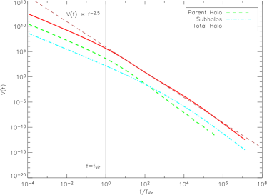
Figure 12: Volume distribution function of phase space density, $v(f)$ as predicted by the parent $+$ substructure model proposed here. Curves for the parent halo and the sub halos were shifted vertically by two decades for clarity. The model $v(f)$ shows a slight hump beyond $f/f_{Vir}=10^{2}$ as compared to the constant slope $v(f)\propto f^{-2.5}$ behavior. This is the point where the subhalo’s contribution to $v(f)$ starts to dominate over the parent halo’s contribution.

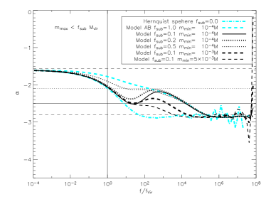
Figure 13: Dependence of slope parameter $\alpha$ on $f$ as predicted by the parent $+$ substructure model proposed here for different values of the parameters, sub halo mass fraction $f_{sub}$ and minimum mass of sub halo $m_{min}$. The profile has a minimum at $\log(f/f_{Vir})\sim 1.5$ and maximum at $\log(f/f_{Vir})\sim 3$. As $f_{sub}$ increases (keeping $m_{min}=10^{-4}M$ constant) the minimum point of $\alpha$ moves up till it matches with with the $f_{sub}=1$ AB Toy model. On the other hand as $m_{min}$ is increased (keeping $f_{sub}=0.1$ constant) the maximum point of $\alpha$ drops down and ultimately it merges with the substructure-less Hernquist profile $f_{sub}=0$.

In both the models it was assumed that the entire halo is made up by superposition of sub halos with a mass function given by $dn/dm\propto m^{-\gamma}$. In the analysis done by De Lucia et al. (2004), where this mass function was determined, the background parent halo which, which accounts about $90\%$ of the total mass, is excluded from the calculation. The parent halo here is not a part of the substructure population. We take this fact into account and develop a model in which we account separately for the contribution of the parent halo. The halo consists of 1) the parent halo with mass $(1-f_{sub})M$ modeled as a Hernquist sphere and 2) the substructure of total mass $f_{sub}M$ which is modeled as a superposition of Hernquist spheres with a mass function of $dn/dm\propto m^{-\gamma}$. To calculate the scale radius $a$ of a sub halo of mass $m$ we use the virial scaling relation $M_{Vir}\propto R_{Vir}^{3}$ which gives $m\propto a^{3}$ (assuming concentration parameter to be same for all sub halos). In Fig. 12 we plot the volume distribution function as predicted by this model for $f_{sub}=0.1,m_{min}=10^{-4}M$. In order to calculate $v(f)$ we employ a semi-analytic technique. We generate a sub halo population corresponding to the given mass function and mass fraction $f_{sub}$ and then for a given value of $f$ we sum the volume contribution of each sub halo along with the parent halo to give the total $v(f)$. The $v(f)$ for each sub halo is determined using Eq. (9) and Eq. (10). The total $v(f)$ as predicted by this model is close to the expected $v(f)\propto f^{-2.5}$ behavior but there is a presence of a slight hump in the high $f$ part. This is similar to what we saw for $\Lambda$CDM halos Fig. 7. In the high $f$ part $v(f)$ is dominated by the substructure component the transition being at around $f/f_{Vir}=10^{2}$. In Fig. 13 we plot the slope parameter $\alpha$ as predicted by the model for various values of $f_{sub}$ and $m_{min}$.

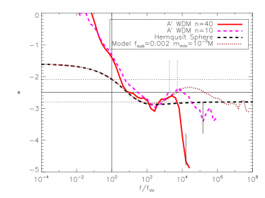
Figure 14: Effect of changing the number of smoothing neighbors on the slope parameter $\alpha$ for a WDM halo. Results are shown for kernel smoothing with smoothing neighbors $n=40$ and $n=10$. The slope parameter $\alpha$ for a Hernquist sphere and a model with $m_{min}=10^{-5}$ and $f_{sub}=0.002$ is also plotted alongside.

Figure 15: The x Vs y and $V_{x}$ Vs $V_{y}$ scatter plot of particles having phase space density above $10^{3}f_{Vir}$ for a warm dark matter halo. In top panels the density is evaluated by using kernel smoothing with 40 smoothing neighbors while in lower panels the density is evaluated using 10 smoothing neighbors.

In Fig. 8 $\alpha(f)$ corresponding to model with parameters $f_{sub}=0.05,m_{min}=10^{-5}M$ is compared against $\alpha(f)$ for simulated halos. It can be seen that the model (analytical profile) is successful in qualitatively explaining the behavior of the simulated halos (namely the dip and the peak) but there is still some difference at the low $f$ end. At the low $f$ end near $f_{Vir}$, parameter $\alpha$ rises much more sharply as compared to the model, even after taking the truncation effect into account.

In (Fig. 14) we show the effect of varying the number of smoothing neighbors on the $\alpha$ profile of a WDM halo. Lowering the number of smoothing neighbors to $10$ makes the slope parameter rise to a peak at the high $f$ end. Since with $n=10$ dispersion in density estimates is high, this also results in a slight flattening of the $\alpha$ profile around $f=f_{Vir}$, where $\alpha$ is found to rise steeply. Plotted alongside is the $\alpha$ profile of the best fit parent $+$ sub halo model. The $\alpha$ profile of the WDM halo is consistent with a model having substructure mass fraction $f_{sub}=0.002$. In Fig. 15 we plot the particles having $f/f_{Vir}>10^{3}$ in both real and velocity space. In top panels the density was estimated using $n=40$ neighbors, while for lower panels the density was estimated using $n=10$ neighbors. It can be seen from the figure that warm dark matter halo is not completely free from substructure. More substructure is resolved using smaller number of smoothing neighbors. The fact that even such a small amount of substructure can be detected demonstrates the superior ability of the estimator in resolving the high density regions. It also suggests that the slope parameter $\alpha$ plotted as a function of $f$ can be used as a sensitive tool to estimate the amount of substructure and and the mass function of sub halos.

To further check the efficiency of the code in reproducing the phase space density of a system with substructure we generated a mock system with $f_{sub}=0.1$ and $m_{min}=10^{-4}$, and calculated its phase space density using EnBiD. The results are shown in Fig. 16 . The sub halos where distributed uniformly inside the virial radius of the parent halo and their center of mass velocity was also chosen so as to have a uniform random distribution within a sphere of radius $V_{Vir}$ in velocity space. For a system modeled with $10^{6}$ particles, the phase space structure till $f=10^{4}f_{Vir}$ is successfully reproduced by using kernel smoothing with $10$ smoothing neighbors. If $40$ smoothing neighbors are used the high density regions are poorly resolved. Lowering the total number of particles in the system also leads to poor resolution at the high $f$ end.

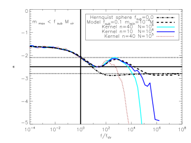
Figure 16: Dependence of slope parameter $\alpha$ on $f$ as recovered by EnBiD from a parent $+$ substructure model. The fraction of mass in the form of substructure is $f_{sub}=0.1$, and the minimum mass of the substructure is $m_{min}=10^{-4}M$, $M$ being the total mass of the system. The theoretically expected slope parameter for the above model and for a Hernquist sphere without any substructure is also plotted alongside. For a system sampled with $10^{6}$ particles, the parameter $\alpha$ can be accurately predicted till $f/f_{Vir}=10^{4}$ using kernel smoothing with $10$ smoothing neighbors.

5 Discussion & Conclusions

We have presented a method for estimation of densities in a multi-dimensional space based on binary space partitioning trees (Ascasibar & Binney, 2005). We implement a node splitting criterion that uses Shannon Entropy as a measure of information available in a particular dimension. The new algorithm makes the scheme metric free and recovers maximum information available from the data with a minimum loss of resolution. In our tests on systems whose density distribution is known analytically, we find significant improvement in estimated densities as compared to earlier algorithms.

We suggest how kernel-based schemes (SPH) or in general any metric based scheme can be implemented within the framework of the new algorithm: the algorithm EnBiD is used to determine the metric at any given point, which has the property that locally the co-variance of the data points has a similar value along all dimensions. Next we incorporate this metric into kernel-based schemes and use them for density estimation. We also show that SPH schemes suffer from a bias in their density estimates. We suggest a prescription that can successfully correct the bias.

As an immediate application, we employ this method to analyze the phase space structure of dark matter halos obtained from N-Body simulation with a $\Lambda$CDM cosmology. We find evidence for slight deviations from the near power law behavior of the volume distribution function $v(f)$ of halos in such simulations. At the high $f$ end there is slight hump and the low $f$ end there is significant flattening. We also analyzed a $WDM$ halo and found that its slope parameter profile $\alpha(f)$ at the high $f$ end is consistent with that of an equilibrium Hernquist sphere having a very small amount of mass ($0.2\%$) in the form of substructure.

In $\Lambda$CDM halos the contribution to the volume distribution function at the high $f$ end is dominated by the presence of significant amount of substructure. We devise a toy model in which the halo is modeled as a Hernquist sphere and the substructure is modeled as a superposition of Hernquist spheres with a fixed mass fraction $f_{sub}$ and a mass function $dn/dm\propto m^{-1.9}$. We demonstrate that this reproduces the behavior of $v(f)$ as seen in simulations.

The behavior of $v(f)$ and $\alpha(f)$ depends upon the parameters $f_{sub}$,mass function $dn/dm$ of sub halos, and $m_{min}$ the minimum mass of the sub halo. Since the mass function of sub halos and their fraction $f_{sub}$ depends upon the power spectrum of initial conditions and on the cosmology adopted, the phase space structure of the halos might have an imprint of cosmology and initial conditions which might be visible in the profile $\alpha(f)$.

Although the simple toy model that we propose here can explain the basic properties of the volume distribution function there is still some difference at the low $f$ end. The flattening at low $f$ end is more pronounced in simulated halos as compared to those of model halos, even after taking the truncation effect into account. Further improvements on the model described include: The toy model assumes that all sub halos obey the same virial scaling relation while in simulation there should be slight dependence on the time of formation of the sub halo. Moreover the sub halos may be tidally truncated and stripped and so their density profile may be different from that of a pure Hernquist sphere (Hayashi et al., 2003; Kazantzidis et al., 2004). Furthermore, there might be a radial dependence on the properties of sub halos. A detailed model which takes into account these effects might help explaining the phase space properties more accurately.

The issue of universality in the behavior of the volume distribution function still deserves further investigation. For the four halos that we have analyzed one of them had a nearly flat $\alpha(f)$ profile and the others showed a characteristic dip at $f\sim 10f_{Vir}$ and a corresponding rise which peaks at around $f\sim 10^{3}f_{Vir}$. Larger samples of halos need to be investigated in order to put these results on a sound statistical basis. The differences that are seen in the properties of halos might be due to varying degree of virialization. The second concern is regarding the role of numerical resolution on the behavior of the volume distribution function. In the model the shape of the $\alpha(f)$ profile depends upon the minimum mass $m_{min}$ of the sub halo used to model the sub halo population. According to the model $\alpha(f)$ has a minimum at around $f/f_{Vir}\sim 10$ and then it rises to a peak at around $f/f_{Vir}\sim 10^{3}$ whose maximum value is determined by the logarithmic slope of the mass function and is given be $-(4-\gamma)$. Beyond this point increasing the resolution should make the $\alpha(f)$ reach a plateau and then fall off once it reaches the resolution limit of the simulation which occurs approximately at $f_{relax}/f_{Vir}\sim 10^{-2}M_{Vir}/m_{p}$. This suggests that a proper convergence study needs to be done to establish the universality in the phase space behavior of the halos. At higher resolution existence of a behavior different from the toy model suggested here would imply that there are some physical processes at work which significantly alter the properties of low mass sub halos and drive the system towards a universal behavior e.g. the one with a constant slope.

Our analysis here shows that the phase space properties of the halos that are roughly consistent with equilibrium spherical models with a given density profile in real space. A question of fundamental importance is regarding the origin of the universal behavior of these density profiles as seen in simulations. A clue to which might be found by studying as to how the system approaches equilibrium. The evolution of the distribution function of collisionless particles is governed by the collisionless Boltzmann equation. Since the coarsely-grained distribution function of collisionless particles can be measured directly with EnBiD, this offers interesting opportunities to study the processes of phase mixing and violent relaxation, which help the system to reach equilibrium. It might be interesting in this context to study the evolution of the volume distribution function of the halos with time.

Another interesting application of this method is to study the distribution function of equilibrium systems e.g. a disk that hierarchically grows inside a halo. One can study the distribution function of these systems and this can in turn be used to construct equilibrium models.

Finally we would like to point out a potential improvement in the code. If the density distribution in any dimension is linearly independent of the other dimensions then this offers an opportunity to further improve the density estimates by measuring the density distributions in different dimensions separately. The concept of mutual information offers one such way to quantify this linear dependence or independence. An algorithm can be developed which can exploit this feature and improve the density estimates in situations where the data offers such an opportunity.

Appendix A Kernel Density Estimate

For the so called kernel density estimate (KDE) a kernel $W$ is defined such that

$$\int W({\bf x,h})d^{d}{\bf x}=1$$ (27)

The density estimate of a discretely set of N particles at a point ${\bf x}$ is given by

$$\rho({\bf x})=\sum_{i}m_{i}W({\bf x_{i}-x,h})$$ (28)

while the probability density $\hat{f}({\bf x})$ is given by

$$\hat{f}({\bf x})=\frac{1}{N}\sum_{i}W({\bf x_{i}-x},{\bf h})$$ (29)

The smoothing parameter ${\bf h}$ is chosen such that it encloses a fixed number of neighbors $N_{smooth}$. Assuming spherical symmetry the kernel can be written in terms of a radial co-ordinate $u$ only. Some of the popular choices are Gaussian function and the B-splines (Monaghan & Lattanzio, 1985). The later is preferred due to its compact support. A $d$ dimensional multivariate bandwidth spherical kernel can be written as

$$W({\bf x},{\bf h})=\frac{f_{d}W_{d}(u)}{\Pi_{i=1}^{d}h_{i}}$$ (30)

where

$$u=\sqrt{\sum_{i=1}^{d}\left(\frac{x_{i}}{h_{i}}\right)^{2}}$$ (31)

and the normalization $f_{d}$ is given by

$$f_{d}=\frac{1}{\int_{0}^{1}W(u)S_{d}u^{d-1}du}$$ (32)

$S_{d}$ being the surface of a unit hyper-sphere in $d$ dimensions $V_{d}$ its volume.

$$S_{d} = 2\pi^{d/2}/\Gamma(d/2)\textrm{\ \ ;\ \ $V_{d}=S_{d}/d$ }$$ (33)

Some popular kernels are given below and their normalizations constants $f_{d}$ are listed in Table. 3

$$W_{Gaussian}(u)=\exp(-u^{2})\textrm{\ \ ;\ }f_{d}=\frac{1}{\pi^{d/2}}$$ (34)

$$W_{Top-Hat}(u)=\left\{\begin{array}[]{ll}1&\ \ 0\leq u\leq 1\\ 0&\ \ \rm{otherwise}\end{array}\right.\textrm{\ \ ;\ }f_{d}=\frac{1}{V_{d}}$$ (37)

$$W_{Spline}(u)=\left\{\begin{array}[]{ll}1-6u^{2}+6u^{3}&\ \ 0\leq u\leq 0.5\\ 2(1-u)^{3}&\ \ 0.5\leq u\leq 1\\ 0&\ \ \rm{otherwise}\end{array}\right.$$ (41)

$$W_{Epanechikov}(u)=\left\{\begin{array}[]{ll}(1-u^{2})&\ \ 0\leq u\leq 1\\ 0&\ \ \rm{otherwise}\end{array}\right.$$ (44)

$$W_{Bi-Weight}(u)=\left\{\begin{array}[]{ll}(1-u^{2})^{2}&\ \ 0\leq u\leq 1\\ 0&\ \ \rm{otherwise}\end{array}\right.$$ (47)

For kernels in product form

$$W({\bf x},{\bf h})=\frac{\Pi_{i=1}^{d}f_{1}W(u_{i})}{\Pi_{i=1}^{d}h_{i}}$$ (48)

where $u_{i}=x_{i}/h_{i}$ and $f_{1}$ is the corresponding one dimensional normalization factor as given by Eq. (32).

Table 3: Normalization constants for various dimensions

Dimension	Normalization $f_{d}$
d	Spline	Epanechnikov	Bi-Weight
1	1.3333369	0.75000113	0.93750176
2	1.8189136	0.63661975	0.95492964
3	2.5464790	0.59683102	1.0444543
4	3.6606359	0.60792705	1.2158542
5	5.4037953	0.66492015	1.4960706
6	8.1913803	0.77403670	1.9350925
7	12.748839	0.95242788	2.6191784
8	20.366416	1.2319173	3.6957561
9	33.380983	1.6674189	5.4191207
10	56.102186	2.3527875	8.2347774

A.1 Optimum Choice of Smoothing Neighbors

If $\hat{f(x)}$ is the estimated probability density of a field $f(x)$ then its mean square error (MSE) can be written in terms of its bias $\beta(x)$ and variance $\sigma(x)$. Bias of an estimate is given by

$$\beta(x) = \langle\hat{f}(x)\rangle-f(x)$$ (49)

while its variance is

$$\sigma^{2}(x) = \langle\left[\hat{f}(x)-\langle\hat{f}(x)\rangle\right]^{2}\rangle$$ (50)

Hence mean square error is given by

$$MSE[\hat{f}(x)] = \langle\left[\hat{f}(x)-f(x)\right]^{2}\rangle$$ (51)

$$= \langle\left[\hat{f}(x)-\langle\hat{f}(x)\rangle+\langle\hat{f}(x)\rangle-f(x)\right]^{2}\rangle$$ (52)

$$= \sigma^{2}(x)+\beta^{2}(x)$$ (53)

To get accurate estimates both bias and variance should be small. Using the fact that

$$\langle\sum_{i=1}^{N}A(x-x_{i})\rangle=N\int A(x-x^{\prime})f(x^{\prime})dx^{\prime}$$ (54)

the bias and variance of an estimator can be calculated by using Eq. (29) and expanding $f(x^{\prime})$ as a Taylor series about $x$. For a $d$ dimensional multivariate kernel density estimate,the bias and variance are given by

$$\beta(x) \approx \frac{h^{2}}{2}Tr[H_{f}(x)]\int u^{2}W_{d}(u)S_{d}u^{d-1}du$$ (55)

where $H_{f}(x)=\frac{\partial^{2}f}{\partial x_{i}\partial x_{j}}$ is the Hessian matrix of function $f(x)$.

$$\sigma^{2}(x) \approx \frac{1}{nh^{d}}f(x)\int W_{d}^{2}(u)S_{d}u^{d-1}du$$ (56)

$$\approx f^{2}(x)\frac{V_{d}}{N_{smooth}}\int W_{d}^{2}(u)S_{d}u^{d-1}du$$ (57)

$$\approx f^{2}(x)\frac{V_{d}}{N_{smooth}}||W_{d}||^{2}_{2}$$ (58)

$||W_{d}||^{2}_{2}$ being the $d$ dimensional $L^{2}$ norm of kernel function $W_{d}(u)$.

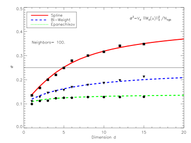
Figure 17: The variance of density estimates, as obtained by kernel smoothing using 100 smoothing neighbors, as a function of number of dimensions. The solid lines are calculated using Eq. (LABEL:eq:sigma) while the points are the $\sigma$ extracted from a Poisson sampled data by applying kernel smoothing.

Lowering $h$ or equivalently lowering $N_{smooth}$ lowers $\beta(x)$ but increases $\sigma(x)$. Ideally the optimum choice of $N_{smooth}$ is given by minimizing the MSE. The bias $\beta$, which depends on the second order derivative of the field, is small for slowly varying fields, hence can be ignored. Since $\sigma(x)\propto 1/\sqrt{N_{smooth}}$, the variance increases as $N_{smooth}$ is decreased. The minimum value of $N_{smooth}$ that is needed to attain a given value of $\sigma(x)$ is the optimum choice of number of neighbors. We define this lower limit on $\sigma$ as $0.25f(x)$. In Fig. 17 $\sigma$ is plotted as a function of number of dimensions $d$ for $N_{smooth}=100$ (assuming $f(x)=1$). The variance as obtained by applying kernel smoothing on a Poisson sampled data with $N_{smooth}=100$ is also shown alongside. They are in agreement. The variance $\sigma$ does not increase exponentially with number of dimensions. Hence the optimum number of neighbors also do not have to grow exponentially with the number of dimensions. This means that even in higher dimensions kernel smoothing can be efficiently done employing a small number of neighbors. In higher dimensions the efficiency of the nearest neighbor search algorithm is the main factor which determines the time required for kernel density estimation. It can also be seen from Fig. 17 that for a fixed number of neighbors the spline kernel gives maximum variance while the Epanechnikov kernel gives the lowest variance. Eq. (LABEL:eq:sigma) can be used to calculate the number smoothing neighbors $N_{smooth}$ required to achieve a given $\sigma$, for any given kernel in any arbitrary dimension. For density estimation with an Epanechnikov kernel in $6$ dimensions, $N_{smooth}=32$ gives a variance of $\sigma=0.22$ which is equivalent to a variance of $0.1$ dex.

A.2 Fraction of Boundary Particles

For a system of $N$ particles uniformly distributed in a spherical region in a $d$ dimensional space the fraction of particles $f_{b}$ that lie on the boundary increases sharply with the number of dimensions $d$. If $l$ is the mean inter-particle separation then $l=(V_{d}r^{d}/N)^{1/d}$ and the fraction $f_{b}$ is given by

$$f_{b} = (S_{d}r^{2}/l^{2})/(V_{d}r^{3}/l^{3})=dl/r=d(V_{d}/N)^{1/d}$$

For $N=10^{6}$, the fraction $f_{b}$ is $0.05$ and $0.79$ for $d=3$ and $d=6$ respectively.

A.3 Anisotropic Kernels

For planar structures which are not parallel to one of the co-ordinate axis one needs to adopt an anisotropic kernel to get accurate results. This is equivalent to a transformation with a rotation and a shear which diagonalizes the covariance matrix and then normalizes the eigenvalues (Shapiro et al., 1996). Let $H$ be a diagonal matrix such that $H_{ii}=h_{i}$ and ${\bf x^{\prime}}=H^{-1}{\bf x}$. If $C({\bf x^{\prime}})$ is the covariance matrix locally at point ${\bf x^{\prime}}$ then the kernel is given by

$$W({\bf x,h}) = \frac{f_{d}}{|D|^{1/2}|H|}W_{d}\left(|D^{-1/2}EH^{-1}{\bf x}|\right)$$ (60)

where $E$ is the eigenvalue matrix that diagonalizes $C$ and $D$ is the corresponding diagonal eigenvalue matrix. To keep the number of smoothing neighbors roughly constant we normalize the eigenvalue matrix, $\mathbf{D}\rightarrow\mathbf{D}/|\mathbf{D}|^{1/d}$, this preserves the smoothing volume. To identify the neighbors that contribute to the density at $\mathbf{x}$ one now needs to select a spherical region with radius ${\bf h^{\prime}}={\bf h}\ \rm{max}(\mathbf{D^{1/2}})$.

A.4 Bias in Spline Kernels

Spline kernels have a bias in their estimated densities i.e. they systematically overestimate the density. This is not present for a regularly distributed data like a lattice or a glass like configuration where the inter-particle separation is constant . This only occurs for a data which has Poisson noise and whose density is measured at the location of the data points. In some sense the bias is due to evaluation of the density at the location of Poisson peaks in the density distribution. The smaller the distance from the center the greater the weight of the kernel. When the density is estimated at the location of the particle the kernel assigns a very high weight to this particle since its distance is zero. Below is shown a simple calculation which demonstrates the bias in a spline kernel as compared to a top hat kernel which is free from such bias.

$$\frac{f}{f_{t}} = \frac{\sum_{i=0}^{i=k}mW_{i}}{\rho_{t}}$$ (61)

$$= \frac{mW_{r=0}+\sum_{i=1}^{i=k}mW_{i}}{\rho_{t}}$$ (62)

Assuming that the top hat kernel gives the correct density $f_{t}=k/(V_{d}h^{d})$. Taking one particle out from the smoothing region should roughly give a density of $\sum_{i=1}^{i=k}mW_{i}=m(k-1)/V_{d}h^{d}$.

$$= \frac{mW_{r=0}+(k-1)m/(V_{d}h^{d})}{km/(V_{d}h^{d})}$$ (64)

$$= 1+\frac{f_{d}V_{d}-1}{k}$$ (65)

It can be seen from Eq. (LABEL:eq:bias) that the bias decreases when the number of smoothing neighbors $k$ is increased. This bias can be removed by displacing the central particle having $r=0$ to $r=hd/(1+d)$, $h$ being the radius of the smoothing sphere, and $d$ the dimensionality of the space. This corresponds to the mean value of radius $r$ of a homogeneous sphere in a $d$ dimensional space . This correction should only be applied if the distribution of data is known to be irregular.

In Fig. 18 kernel density estimates with and without bias correction are shown for a system of $N=10^{5}$ particles distributed uniformly in a 6 dimensional space with periodic boundaries. In left panel the probability distribution $P(\log(f/f_{t}))$ is plotted with and without bias correction, for kernel density estimate obtained using a spline function and smoothing neighbors $n=64$. In right panel the probability distributions are plotted for kernel density estimates obtained using an Epanechnikov function and smoothing neighbors $n=32$. The bias given by mean $<x>$ of the best fit Gaussian distribution is also plotted alongside. According to Eq. (LABEL:eq:bias), in a $6$ dimensional space for spline kernels with neighbors $k=64$ the bias is $<\log(f_{sp}/f_{t})>=0.21$ and for Epanechnikov kernel with $k=32$ the bias is $<\log(f_{Ep}/f_{t})>=0.04$. These values are close to those shown in Fig. 18 for uncorrected estimates. The Epanechnikov kernel function has less bias than the spline kernel function. After correction, for both the kernels, the bias is considerably reduced.

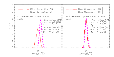
Figure 18: Kernel density estimates with and without bias correction. are shown for a system of $N=10^{5}$ particles distributed uniformly in a 6 dimensional space with periodic boundaries. Probability distribution $P(\log(f/f_{t}))$ is plotted for spline kernel with smoothing neighbors $n=64$ (left panel ) and Epanechnikov kernel with $n=32$ (right panel). The mean $<x>$ and dispersion $\sigma_{x}$ of the best fit Gaussian distribution to $x=\log(f/f_{t})$, is also shown alongside.

References

- Arad et al. (2004) Arad, I., Dekel, A., Klypin, A. 2004, MNRAS, 353, 15
- Ascasibar & Binney (2005) Ascasibar, Y., Binney, J. 2005, MNRAS, 356, 872
- Bernardeau & van de Weygaert (1996) Bernardeau, F., & van de Weygaert, R. 1996, MNRAS, 279, 693
- Binney & Tremaine (1987) Binney, J., Tremaine S., 1987, Galactic Dynamics (Princeton Univ Press)
- Binney (2004) Binney, J. 2004, MNRAS, 350, 939
- Couchman (1991) Couchman, H. M. P. 1991, ApJ, 368, L23
- De Lucia et al. (2004) De Lucia, G., Kauffmann, G., Springel, V., White, S. D. M., Lanzoni, B., Stoehr, F., Tormen, G., & Yoshida, N. 2004, MNRAS, 348, 333
- Diemand et al. (2004) Diemand, J., Moore, B., Stadel, J., & Kazantzidis, S. 2004, MNRAS, 348, 977
- Gershenfeld (1999) Gershenfeld N., 1999, The Nature of Mathematical Modeling. Cambridge University Press
- Gingold & Monaghan (1977) Gingold, R. A., & Monaghan, J. J. 1977, MNRAS, 181, 375
- Hayashi et al. (2003) Hayashi, E., Navarro, J. F., Taylor, J. E., Stadel, J., & Quinn, T. 2003, ApJ, 584, 541
- Hernquist (1990) Hernquist, L. 1990, ApJ, 356, 359
- Hockney & Eastwood (1981) Hockney, R. W., & Eastwood,J. W. 1981,Computer simulations using particles, (New York: McGraw-Hill)
- Kazantzidis et al. (2004) Kazantzidis, S., Mayer, L., Mastropietro, C., Diemand, J., Stadel, J., & Moore, B. 2004, ApJ, 608, 663
- Kravtsov et al. (1997) Kravtsov, A. V., Klypin, A. A., & Khokhlov, A. M. 1997, ApJS, 111, 73
- Loftsgaarden & Quesenberry (1965) Loftsgaarden D. O., and Quesenberry, C. P., 1948 ,A non parametric estimate of a multivariate density function. Annal. Math. Statist., 36:1049-1051.
- Lucy (1977) Lucy, L. B. 1977, AJ, 82, 1013
- MacKay (2003) MacKay D. J. C., 2003, Information Theory,Inference, and Learning Algorithms. Cambridge University Press
- Melchiorri, Bode, Bahcall, & Silk (2003) Melchiorri, A., Bode, P., Bahcall, N. A., & Silk, J. 2003, ApJ, 586, L1
- Monaghan & Lattanzio (1985) Monaghan, J. J., & Lattanzio, J. C. 1985, A&A, 149, 135
- Monaghan (1992) Monaghan, J. J. 1992, ARA&A, 30, 543
- Navarro et al. (2004) Navarro, J. F., et al. 2004, MNRAS, 349, 1039
- Navarro, Frenk, & White (1996) Navarro, J. F., Frenk, C. S., & White, S. D. M. 1996, ApJ, 462, 563
- Navarro, Frenk, & White (1997) Navarro, J. F., Frenk, C. S., & White, S. D. M. 1997, ApJ, 490, 493
- Okabe et al. (1992) Okabe, A., Boots, B., & Sugihara, K. 1992, Wiley Series in Probability and Mathematical Statistics, Chichester, New York: Wiley, 1992,
- Okabe (2000) Okabe, A. 2000, Spatial tessellations : concepts and applications of voronoi diagrams. 2nd ed. By Atsuyuki Okabe …[et al] Chichester ; Toronto : John Wiley & Sons, 2000.,
- Press et al. (1992) Press, W. H., Teukolsky, S. A., Vetterling, W. T., & Flannery, B. P. 1992, Cambridge: University Press, —c1992, 2nd ed.,
- Schaap & van de Weygaert (2000) Schaap, W. E., & van de Weygaert, R. 2000, A&A, 363, L29
- Shannon (1948) Shannon, C. E., 1948 ,A mathematical theory of communication. Bell System Tech. J., 27:379–423.
- Shannon (1949) Shannon C. E., & Weaver W., 1949, The Mathematical Theory of Communication. University of Illinois Press.
- Shapiro et al. (1996) Shapiro, P. R., Martel, H., Villumsen, J. V., & Owen, J. M. 1996, ApJS, 103, 269
- Silverman (1986) Silverman, B. W. 1986, Monographs on Statistics and Applied Probability, London: Chapman and Hall, 1986,
- Spergel et al. (2003) Spergel, D. N. et al. 2003, ApJS, 148, 175
- Springel, Yoshida, & White (2001) Springel, V., Yoshida, N., & White, S. D. M. 2001, New Astronomy, 6, 79
-
Stadel (1995)
Stadel, J. 1995,
http://www-hpcc.astro.washington.edu/tools/smooth.html