Inhomogeneous systematic signals in cosmic shear observations

Abstract

We calculate the systematic errors in the weak gravitational lensing power spectrum which would be caused by spatially varying calibration (i.e., multiplicative) errors, such as might arise from uncorrected seeing or extinction variations. The systematic error is fully described by the angular two-point correlation function of the systematic in the case of the 2D lensing that we consider here. We investigate three specific cases: Gaussian, “patchy” and exponential correlation functions. In order to keep systematic errors below statistical errors in future LSST-like surveys, the spatial variation of calibration should not exceed $3\%$ rms. This conclusion is independently true for all forms of correlation function we consider. The relative size the E- and B-mode power spectrum errors does, however, depend upon the form of the correlation function, indicating that one cannot repair the E-mode power spectrum systematics by means of the B-mode measurements.

I Motivation

The power spectrum of the weak gravitational lensing distortions of background galaxies is quite directly related to the power spectrum of intervening matter (Miralda-Escude, 1991; Kaiser, 1992). The weak lensing (WL) power spectrum depends upon the linear and non-linear rates of growth of structure since recombination, and upon the redshift-distance relation produced by the expansion. These dependences, plus the straightforward theoretical framework, make WL a very attractive tool for the constraint of the post-recombination Universe, e.g. dark energy. Current 5–10% measurements of the WL power spectrum have already begun to place interesting constraints (Jarvis et al., 2005), and very much larger-scale projects are planned to reduce the statistical errors on the WL signal to 1 part in $10^{3}$ or lower.

To reap the benefits of these large surveys, systematic errors must be well below the small expected statistical errors. WL measurements are subtle and difficult compared to most astronomical data analyses. There are no “standard lenses” on the sky, so calibration of the WL shear data is a significant worry. The finite point spread function (PSF) width tends to circularize the appearance of background galaxies, squelching the WL shear signal. This must be corrected analytically, and any errors in this process, or inaccuracies in the estimate of the PSF size, will lead to calibration errors. Huterer et al. (2005) investigate the effect of overall mean shear calibration errors on cosmological parameter estimation. It is also likely, however, that there will be spatially varying calibration errors that are larger than the error in the mean calibration. For example, as the PSF size $\sigma_{\star}$ varies during a ground-based survey, the resolution parameter $R\equiv 1-\frac{\sigma^{2}_{\star}}{\sigma^{2}_{g}}$ of the galaxies will vary (here $\sigma_{g}$ is the angular size of a target galaxy). If we fail to track this variation properly, the inferred shear will be modulated by a factor $(1-\delta R(\bm{\theta})/R(\bm{\theta}))$ (Bernstein and Jarvis, 2002). In this paper we calculate the effect of spatially varying calibration errors upon the measured power spectrum, and determine criteria on these systematic errors which will have to be met if they are to be made negligible in future surveys.

Other spatially varying errors could arise from photometric errors or Galactic extinction which will modulate the effective depth of the survey. Both effects may lead to errors in the (photometric) redshift estimation and source galaxy distribution, see e.g. (Jarvis et al., 2003), which would in turn lead to local modulation of the observed shear. While a modulation of redshift depth is not strictly equivalent to a multiplicative modulation of shear, our calculations will still permit an estimate of the level at which depth modulations become significant.

The lensing shear of sources at some redshift $z_{s}$ is a 2-component tensor function of the angular variable $\bm{\theta}$. As reviewed briefly below, the shear field can be divided into “E” and “B” modes corresponding to curl-free and divergence-free deflections, with corresponding power spectra $P_{E}(l)$ and $P_{B}(l)$ for stationary isotropic fields. Gravitational deflections, being derived from the scalar potential, will produce only E-mode power in the weak limit. It is therefore $P_{E}(l)$ that will be used for cosmological constraints, with the B mode serving as the “canary in the coal mine” to alert us to potential non-gravitational sources of systematic error. A spatially varying scalar calibration factor will alter the amplitude of the E-mode power and convert some into B-mode power. In §III we quantify this effect in terms of the 2-point statistics of the calibration systematic. In §IV we present solutions using several models for the systematic error, and show how the deleterious effects are in general determined just by the rms amplitude and characteristic angular scale of the calibration errors. §V summarizes the results and the requirements upon future surveys that can be derived from these results.

Some related calculations exist in the literature. Schneider et al. (2002) investigate the B-mode signal that is created by inhomogeneous source distributions, using a formalism similar to that employed here. We note that the inhomogeneous-source effect can be avoided by considering only cross-correlations between source bins that are disjoint in redshift. The calibration inhomogeneity that we analyze here will likely not be so easily avoided. Vale et al. (2004) conduct a numerical test of calibration inhomogeneity by modulating the shear seen in a ray-tracing simulation, and then calculating the resultant power spectra. We will test our analytic results against their simulated data.

A rough target for calibration systematics is that their effect on $P_{E}(l)$ be smaller than the expected statistical errors. For a single-screen lens analysis, the uncertainty in $P_{E}(l)$ averaged over an interval $\Delta\ln l=1$ is $l^{-1}f_{\rm sky}^{-1/2}P_{E}(l)$ in the sample-variance limit. So for ambitious surveys with $f_{\rm sky}\gtrsim 0.5$, the power spectrum statistical errors are $\approx 1$ part in $10^{3}$ at $l=1000$. At higher $l$, the uncertainties due to shape noise and inaccuracies in the non-linear clustering theory will become important. The tolerances may be tighter when one examines the impact of power-spectrum tomography rather than just a single power spectrum. So a good goal is to have the calibration-induced error $\Delta P_{E}(l)$ be $\leq 10^{-4}P_{E}(l)$.

II Shear field decomposition into E and B modes

Decomposition of a spin-2 field, such as shear or the Stokes parameters, into curl-free and divergence-free part was suggested to be useful for weak gravitational lensing studies by Stebbins (1996), and for cosmic microwave background (CMB) polarization by Kamionkowski et al. (1997) and Zaldarriaga and Seljak (1997). Crittenden et al. (2002) and Schneider et al. (2002) study its use in revealing non-gravitational signals in weak lensing surveys. We briefly review the decomposition of the shear field into independent E and B modes, following the notation of Schneider et al. (2002).

The gravitational lens equation in the one-screen approximation relates the detected direction $\bm{\theta}$ of photons on the sky to the (unobservable) direction $\bm{\beta}$ of photons emitted by a source: $\bm{\Delta}=\bm{\theta}-\bm{\beta}$, where $\bm{\Delta}$ is the deflection angle scaled by a factor depending on the angular diameter distances in the observer-lens-source system (Bartelmann and Schneider, 2001). The gradient of the deflection field, being a tensor of rank two, is usually decomposed locally into the trace, symmetric traceless part, and antisymmetric part as follows $\Delta_{i,j}=\kappa\,\delta_{ij}+\gamma_{ij}+\omega\,\epsilon_{ij}$, where the shear tensor $\gamma_{ij}$ is symmetric and $\epsilon_{ij}$ is the Levi-Civita symbol in two dimensions. We denote partial derivatives with respect to directions in the tangent plane on the sky in a standard fashion by a comma. Thus we may express the convergence $\kappa$ and the rotation $\omega$ as linear combinations of derivatives of the deflection angle: $2\kappa=\Delta_{1,1}+\Delta_{2,2}$, $2\omega=\Delta_{1,2}-\Delta_{2,1}$. Also, the shear components $(\gamma_{1},\gamma_{2})$, defined as $\gamma_{1}\equiv\gamma_{11}=-\gamma_{22}$, $\gamma_{2}\equiv\gamma_{12}=\gamma_{21}$, may be written as $2\gamma_{1}=\Delta_{1,1}-\Delta_{2,2}$, $2\gamma_{2}=\Delta_{1,2}+\Delta_{2,1}$. Moreover, we can write the deflection field as a sum of curl free and divergence free parts $\bm{\Delta}=\bm{\Delta}_{+}+\bm{\Delta}_{\times}$ which can be expressed as the gradient of a scalar potential $\phi_{+}$ and the curl of a pseudoscalar potential $\phi_{\times}$ respectively (Stebbins, 1996). We designate as “E-mode” the curl-free deflection $\bm{\Delta}_{+}$, which resembles an electric field pattern, and can be due to the mass distribution. It produces the tangential shear pattern $\gamma_{+}$ (Stebbins, 1996). On the other hand, the divergence-free “B-mode” deflection $\bm{\Delta}_{\times}$ resembles a magnetic field pattern. This mode reveals in measurements as a “radial” shear $\gamma_{\times}$ (i.e., $\gamma_{+}$ rotated by $45^{\circ}$) and it cannot be generated by lensing in the single-screen approximation. The potentials $\phi_{+}$ and $\phi_{\times}$ are closely related to the convergence $\kappa$ and rotation $\omega$ via the Poisson equation, $\nabla^{2}\phi_{+}=2\,\kappa$ and $\nabla^{2}\phi_{\times}=2\,\omega$. Since the single-screen approximation is thought to be valid in cosmological situations (Van Waerbeke and Mellier, 2003), gravitational lensing information is confined to the E mode while the B mode should be zero. Thus the presence of non-zero B mode would be due to breaking of the single-screen approximation or, more importantly, to a variety of processes not related directly to lensing, such as measurement calibration errors (Hirata and Seljak, 2003; Van Waerbeke et al., 2005; Jarvis and Jain, 2004), clustering of source galaxies (Schneider et al., 2002), or their intrinsic alignments (Heymans and Heavens, 2003). For a more thorough discussion of E/B-mode decomposition see Crittenden et al. (2002).

In order to quantify the contribution of systematic uncertainties to the E and B mode power spectra we introduce a pair of two-point correlation functions $\xi^{\gamma}_{+}(\theta)$ and $\xi^{\gamma}_{-}(\theta)$, following Schneider et al. (2002). They are linear combinations of correlation functions of E and B components of the shear, defined for each pair of galaxies with respect to the preferred coordinate system in which their positions are $\bm{\theta}_{1}=(0,0)$ and $\bm{\theta}_{2}=(\theta,0)$:

$$\xi^{\gamma}_{\pm}(\theta)=\left<\gamma_{1}(\bm{\theta}_{1})\,\gamma_{1}(\bm{\theta}_{2})\right>\pm\left<\gamma_{2}(\bm{\theta}_{1})\,\gamma_{2}(\bm{\theta}_{2})\right>.\\$$ (1)

Moreover, the correlation functions (1) can be expressed as follows in terms of E and B-mode power spectra, $P_{E}(l)$ and $P_{B}(l)$, defined as $\left<\kappa(\bm{l})\kappa(\bm{l^{\prime}})\right>\equiv\left(2\pi\right)^{2}\delta_{\rm D}(\bm{l}+\bm{l^{\prime}})\,P_{E}(l)$ and $\left<\omega(\bm{l})\omega(\bm{l^{\prime}})\right>\equiv\left(2\pi\right)^{2}\delta_{\rm D}(\bm{l}+\bm{l^{\prime}})\,P_{B}(l)$:

$$\xi^{\gamma}_{\pm}(\theta)=\frac{1}{2\pi}\int_{0}^{\infty}dl\,l\,\left(P_{E}(l)\pm P_{B}(l)\right)\,J_{0,4}(l\theta).$$ (2)

We can invert those relations and obtain power spectra expressed in terms of the correlation functions [in what follows we use a convention that upper sign in the sum on the right hand side refers to E-mode power spectrum, lower to B-mode]:

$$P^{\gamma}_{E,B}(l)=\pi\int_{0}^{\infty}d\theta\,\theta\,\left[\xi^{\gamma}_{+}(\theta)\,J_{0}(l\theta)\pm\xi^{\gamma}_{-}(\theta)\,J_{4}(l\theta)\right].$$ (3)

We do not consider cross-power spectrum of E and B modes as it will vanish due to parity conservation (Schneider et al., 2002).

III Effect of systematics on E/B power spectra

Ideally, we would like to measure the shear field $\bm{\gamma}(\bm{\theta})$ directly. What we observe, however, is the coherent ellipticity induced on an ensemble of galaxies, which (a) is defined by the distortion $\bm{g}=\bm{\gamma}/(1-\kappa)$; (b) is imparted on galaxies that are not intrinsically circular, and (c) are viewed through a finite point-spread function (PSF). The measured shear field $\bm{d}(\bm{\theta})$ will in practice be modulated or contaminated by various observational effects (Van Waerbeke and Mellier, 2003). Although techniques for shear extraction from galaxy images have been extensively developed and tested (Kaiser et al., 1995; Bernstein and Jarvis, 2002; Hirata and Seljak, 2003), there remain imperfections which can be detrimental to precision cosmology.

Throughout the paper we assume that the observed field is related to the true shear field by a position-dependent multiplicative scalar factor $1+\epsilon(\bm{\theta})$ such as will result from a misestimation of the “resolution” (Bernstein and Jarvis, 2002) or “shear polarizability” (Kaiser et al., 1995). The systematic field $\epsilon(\bm{\theta})$ is a random field assumed to have zero mean and described to the lowest interesting order by the two-point correlation function. Thus we express the observed field in terms of the shear and the systematics fields as

$$\bm{d}(\bm{\theta})=(1+\epsilon(\bm{\theta}))\,\bm{\gamma}(\bm{\theta}).$$ (4)

This relation is local in real space, so it is going to couple modes of the shear field in the Fourier space, i.e. have some non-local effect on the relevant power spectra. We assume that the shear field $\bm{\gamma}$ due to massive structures in the Universe is uncorrelated with systematics field $\epsilon(\bm{\theta})$, which is a Galactic or instrumental foreground. The observed two-point correlation function $\xi^{d}(\theta)$ can in this case be written as

$$\xi^{d}(\theta) \equiv \left<{\bm{d}}(\bm{\phi})\,{\bm{d}}(\bm{\phi}+{\bm{\theta}})\right>$$ (5)

$$= (1+\left<\epsilon(\bm{\phi})\,\epsilon(\bm{\phi}+{\bm{\theta}})\right>)\,\left<{\bm{\gamma}}(\bm{\phi})\,{\bm{\gamma}}(\bm{\phi}+{\bm{\theta}})\right>$$ (6)

$$= \left(1+\xi^{\epsilon}(\theta)\right)\,\xi^{\gamma}(\theta).$$ (7)

We have introduced two-point correlation functions $\xi^{\gamma}(\theta)$ for the shear field and $\xi^{\epsilon}(\theta)$ for the systematics field. For simplicity we will assume that the systematics field $\epsilon({\bm{\theta}})$ is homogeneous and isotropic. In practice the assumption of isoptropy is not restrictive, as the effects of an anisotropic systematic could be approximated to first order by considering the azimuthally averaged correlation function.

Correlation functions for the distortion field, $\xi^{d}_{+}(\theta)$ and $\xi^{d}_{-}(\theta)$, may be expressed as products of the correlation functions for the shear and systematics $\xi^{d}_{\pm}(\theta)=\left(1+\xi^{\epsilon}(\theta)\right)\xi^{\gamma}_{\pm}(\theta)$ which follow from eqs. (1) and (7). We can rewrite eq. (3) in terms of the distortion instead of the shear and then account for systematic signals $\epsilon({\bm{\theta}})$. We split the observed E and B mode power spectra $P^{d}_{E,B}(l)$ into two contributions as follows

$$P^{d}_{E,B}(l)=P^{\gamma}_{E,B}(l)+\Delta P^{\epsilon}_{E,B}(l),$$ (8)

where the term $P^{\gamma}_{E,B}(l)$ is E mode (B mode) power spectrum of the shear and $\Delta P^{\epsilon}_{E,B}(l)$ represents the contributions to the E mode (B mode) power due to systematic signals. We focus on these error terms in the remainder of the paper. Using eqs. (3) and (8) they can be written as

$$\Delta P^{\epsilon}_{E,B}(l)=\pi\int_{0}^{\infty}d\theta\theta\xi^{\epsilon}(\theta)\left[\xi^{\gamma}_{+}(\theta)J_{0}(l\theta)\pm\xi^{\gamma}_{-}(\theta)J_{4}(l\theta)\right].$$ (9)

We assume that the shear correlation functions $\xi^{\gamma}_{\pm}$ receive contribution from E mode only, i.e. $P^{\gamma}_{E}(l)=P_{\kappa}(l)$, $P^{\gamma}_{B}(l)\equiv 0$, since B-mode cosmological contributions are expected to be a few orders of magnitude smaller on scales $>1^{\prime}$ (Schneider et al., 2002). The systematic errors $\Delta P_{E,B}(l)$ to E and B mode power spectra can be written as integrals over the convergence power spectrum $P_{\kappa}(l)$ with a window function $W_{E,B}(l,q)$:

$$\Delta P_{E,B}(l)=\int_{0}^{\infty}dq\,q\,P_{\kappa}(q)\,W_{E,B}(l,q),$$ (10)

where the window function depends solely on the correlation function $\xi^{\epsilon}$ of the systematic modulation, and is given by

$$W_{E,B}=\frac{1}{2}\int_{0}^{\infty}d\theta\theta\xi^{\epsilon}(\theta)\left[J_{0}(l\theta)J_{0}(q\theta)\pm J_{4}(l\theta)J_{4}(q\theta)\right].$$ (11)

In the limit of a systematic that is completely correlated across the entire observation, i.e. a constant calibration error, we have $\xi^{\epsilon}(\theta)=\Sigma^{2}$, where $\Sigma^{2}$ is the variance of the calibration error. In this limit we obtain $W_{E}(l,q)=\Sigma^{2}\,q^{-1}\delta_{\rm D}(l-q)$ and $W_{B}(l,q)\equiv 0$, where we have used an integral relation for the Bessel functions $\int_{0}^{\infty}d\theta\,\theta\,J_{n}(l\,\theta)\,J_{n}(q\,\theta)=q^{-1}\,\delta_{\rm D}(q-l)$ (Abramowitz and Stegun, 1965). Thus the error contributions to E/B power spectra are $\Delta P_{E}(l)=\Sigma^{2}P_{\kappa}(l)$ and $\Delta P_{B}(l)=0$ in this case, and there is no conversion of E power to B power, as expected.

Numerical simulations of calibration inhomogeneity in (Vale et al., 2004) are presented in terms of the aperture mass statistics $M_{\rm ap}(R)$ and $M_{\times}(R)$ with compensated filter defined in (Schneider et al., 1998; Bartelmann and Schneider, 1999). We produce analytic predictions for inhomogeneous calibration errors for comparison with the numerical results of (Vale et al., 2004) using the same filter as they did.

IV Modeling of systematics

We consider several potentially useful models of the correlation function of the systematic signal $\xi^{\epsilon}(\theta)$ and we examine the dependence of E and B mode power spectra (10) on the characteristics of $\xi^{\epsilon}(\theta)$. The correlation functions considered here are analytically tractable and able to describe a wide variety of random processes leading to systematic signals. Each correlation function considered here is assumed to describe a stationary, isotropic random field. We assume that the systematic field has a finite variance $\Sigma^{2}$. Equation (11) shows that $\Delta P_{E,B}(l)\propto\Sigma^{2}$ if $\Sigma^{2}$ is a prefactor to some otherwise fixed functional form for $\xi^{\epsilon}$. Moreover, a correlation function in 2-D has to be bounded from below by a global minimum value of the Bessel function $J_{0}(x)$. This condition is met by our models because they are assumed to be non-negative (Ripley, 1981).

We also introduce for each correlation function a characteristic scale $R_{1/2}$ where the correlation function drops to 50% of its zero-lag value $\Sigma^{2}$.

IV.1 Gaussian family

As a first model let us consider correlation function having a Gaussian shape with characteristic scale $\theta_{0}$

$$\xi^{\epsilon}(\theta)=\Sigma^{2}\,e^{-\frac{\theta^{2}}{2\theta_{0}^{2}}}.$$ (12)

We have $R_{1/2}^{2}=2\,\theta_{0}^{2}\,\ln 2$ for the Gaussian. The Gaussian is chosen because they are usually easy to handle analytically. In this case an integral over scale $\theta$ in eq. (11) can be done analytically (Gradshteyn and Ryzhik, 2000) and we obtain the following window function

$$W_{E,B}(l,q)=\frac{\Sigma^{2}\,\theta_{0}^{2}}{2}\,e^{-\frac{1}{2}\theta_{0}^{2}(l^{2}+q^{2})}\left[I_{0}(\theta_{0}^{2}\,l\,q)\pm I_{4}(\theta_{0}^{2}\,l\,q)\right],$$ (13)

where $I_{0}(x)$ and $I_{4}(x)$ are the modified Bessel functions of the first kind of zeroth and fourth order respectively (Abramowitz and Stegun, 1965). Because of the exponential growth of $I_{0}(x)$ and $I_{4}(x)$ with $x$ it is useful to rearrage terms in (13) and rewrite this equation as

$$W_{E,B}(l,q)=\frac{\Sigma^{2}\,\theta_{0}^{2}}{2}\,e^{-\frac{1}{2}\theta_{0}^{2}(l-q)^{2}}\left[{\hat{I}}_{0}(\theta_{0}^{2}\,l\,q)\pm{\hat{I}}_{4}(\theta_{0}^{2}\,l\,q)\right],$$ (14)

where we have introduced functions ${\hat{I}}_{n}(x)=e^{-x}I_{n}(x)$.

The large-scale amplitude of $W_{E,B}(l,q)$ can be derived by noting the asymptotic behavior of the modified Bessel function for small arguments: $I_{0}(x)\sim 1$ and $I_{4}(x)\sim x^{4}/384$ if $x\ll 1$. Thus for scales large compared to $R_{1/2}$ when $\theta_{0}\,l\ll 1$, we obtain $W_{E,B}(l,q)\sim\frac{1}{2}\Sigma^{2}\,\theta_{0}^{2}\,e^{-\frac{1}{2}\theta_{0}^{2}\,l^{2}}$. When we consider power spectra $\Delta P_{E,B}(l)$ in this regime we get the following expression

$$\Delta P_{E,B}(l) \approx \frac{1}{2}\Sigma^{2}\theta_{0}\int_{0}^{\infty}dq\,q\,P_{\kappa}(q)\,e^{-\frac{1}{2}\theta_{0}^{2}\,q^{2}}$$ (15)

$$\approx \frac{1}{2}\Sigma^{2}P_{\kappa}\left(l=\frac{1}{\theta_{0}}\right).$$ (16)

In the above we used the fact that the function $q\,\theta_{0}\,e^{-1/2\theta_{0}^{2}\,q^{2}}$ has a maximum at $q=1/\theta_{0}$ and can be regarded narrow around its maximum. The error we make using this approximation is less than $10\%$ for $R_{1/2}=1^{\circ}$ and $40\%$ for $R_{1/2}=1^{\prime}$.

For small scales where $\theta_{0}\,l\gg 1$ and $\theta_{0}\,q\gg 1$, we may use another asymptotic formula for modified Bessel functions which leads to ${\hat{I}}_{n}(x)\sim\sqrt{2\pi}\,x^{-1/2}$ (Abramowitz and Stegun, 1965). This limit is safely taken when the argument of ${\hat{I}}_{0}$ or ${\hat{I}}_{4}$ is greater than $1$ or $100$, respectively. Thus we obtain from (14) for small scales the following

$$\left.\begin{array}[]{l}W_{E}(l,q)\\ W_{B}(l,q)\end{array}\right\}\sim\frac{\Sigma^{2}\theta_{0}^{2}}{\sqrt{2\pi\theta_{0}^{2}lq}}e^{-\frac{1}{2}\theta_{0}^{2}(l-q)^{2}}\left\{\begin{array}[]{l}1-\frac{4}{\theta_{0}^{2}lq},\\ \frac{31}{8\theta_{0}^{2}lq}.\end{array}\right.$$ (17)

The asymptotic expression (17) is useful when computing the small-scale systematics contribution to E and B-mode power spectra (10). Due to the exponential term in the window function (17) it is effectively a Dirac delta function $\delta_{\rm D}(l-q)$. Thus we can write eq. (10) as

$$\left.\begin{array}[]{l}\Delta P_{E}(l)\\ \Delta P_{B}(l)\end{array}\right\}\sim\Sigma^{2}\,P_{\kappa}(l)\left\{\begin{array}[]{l}1,\\ \frac{31}{8}\theta_{0}^{-2}l^{-2}.\end{array}\right.$$ (18)

if we consider small scales compared to $R_{1/2}$. The asymptotic behavior of E and B-mode systematics power spectra is seen in fig. 1. It is notable that, for sufficiently large $l$, the systematic E-mode contribution $\Delta P_{E}$ is simply a factor $\Sigma^{2}$ of the convergence power spectrum $P_{\kappa}(l)$. Moreover, $\Delta P_{E}$ follows the shape of $P_{\kappa}(l)$, whereas the B-mode contribution $\Delta P_{B}$ drops rapidly.

IV.2 Patchy

Let us consider a systematic signal $\epsilon(\bm{\theta})$ which is perfectly correlated within circular patches of diameter $\theta_{0}$ on the sky. This kind of systematics could arise if the survey is a mosaic of (circular) telescope pointings, and each pointing has a constant calibration error that is statistically independent of all other pointings. For example, the impact of time-variable atmospheric seeing on galaxy shape measurements could produce such a pattern. Assuming such a model, we can compute the correlation function $\xi^{\epsilon}(\theta)$ (independent of the specific distribution (pdf) of $\epsilon(\bm{\theta})$ amplitude)

$$\xi^{\epsilon}\left(\theta\right)=\Sigma^{2}\left[1-\frac{2}{\pi}\left(\arcsin\frac{\theta}{\theta_{0}}+\frac{\theta}{\theta_{0}}\sqrt{1-\frac{\theta^{2}}{\theta_{0}^{2}}}\right)\right]{\mathrm{H}}(\theta_{0}-\theta)$$ (19)

where ${\mathrm{H}}$ is the Heaviside step function and $R_{1/2}\approx 0.404\theta_{0}$. This type of correlation and its effect on E mode signal degradation and B mode generation were studied by Vale et al. (2004) using ray-tracing simulations (their “sharp modulation” model). Although they assumed square areas of correlation (the shape of CCD detectors), our analytic model should match this well if we perform angular averaging over the square pattern to get an isotropic correlation function.

In this case a closed form for the window function is not attained, so we have to rely on numerical integration. We can deal analytically with the window function (11) in the limit of small scales $l\theta_{0}\gg 1$ and $q\theta_{0}\gg 1$. For this purpose we can approximate (19) by $\xi^{\epsilon}\left(\theta\right)\approx\Sigma^{2}\left[1-\theta/\theta_{0}\right]$ where $\theta_{0}=2R_{1/2}$. Let us use asymptotic formulae for the Bessel functions for large arguments (Abramowitz and Stegun, 1965) and write the E mode window function as follows:

$$W_{E}(l,q) \approx \frac{\Sigma^{2}}{\pi\sqrt{lq}}$$ (20)

$$\!\!\!\!\!\!\!\!\!\!\!\!\!\!\!\!\!\!\!\!\!\!\!\!\!\!\!\!\!\!\!\!\!\times\int_{0}^{\infty}d\theta\left(1-\frac{\theta}{\theta_{0}}\right)\cos\left(l\theta-\frac{\pi}{4}\right)\cos\left(q\theta-\frac{\pi}{4}\right).$$

Using the formulae for addition of cosines and subsequently perform elementary integration leads us to

$$W_{E}(l,q) \approx \frac{\Sigma^{2}\theta_{0}}{\pi\sqrt{lq}}$$ (21)

$$\!\!\!\!\!\!\!\!\!\!\!\!\!\!\!\!\!\!\!\!\!\!\!\!\!\!\!\!\times\left[\frac{1-\cos\theta_{0}\left(l-q\right)}{\theta_{0}^{2}(l-q)^{2}}+\frac{1-\sin\theta_{0}\left(l+q\right)}{\theta_{0}^{2}(l+q)^{2}}\right].$$

Thus in the interesting case of small scales main contribution to the window function comes from $l\approx q$ which leads to

$$W_{E}(l,q)\sim\frac{\Sigma^{2}\theta_{0}}{2\pi l}\frac{\sin^{2}\frac{\theta_{0}\left(l-q\right)}{2}}{\frac{\theta_{0}^{2}\left(l-q\right)^{2}}{4}}\sim\Sigma^{2}l^{-1}\delta_{\rm D}(l-q).$$ (22)

The B-mode window tends to zero because of the identical asymptotic behavior of $J_{0}$ and $J_{4}$. Thus in the small scales limit we have $\Delta P_{E}(l)\sim\Sigma^{2}\,P_{\kappa}(l)$, $\Delta P_{B}(l)\rightarrow 0$ which was the case for a Gaussian correlations as well.

IV.3 Generalized exponential family

A broad class of correlation functions can be described by a generalized exponential family (Ripley, 1981) as follows

$$\xi^{\epsilon}(\theta)=\frac{\Sigma^{2}}{2^{\nu-1}\Gamma(\nu)}\left(\frac{\theta}{\theta_{0}}\right)^{\nu}K_{\nu}\left(\frac{\theta}{\theta_{0}}\right),$$ (23)

where $K_{\nu}(x)$ is the modified Bessel function of the second kind, $\theta_{0}$ is a characteristic scale and $0<\nu<1$. For $\nu=1/2$ we obtain an exponential correlation function $\xi^{\epsilon}(\theta)=\Sigma^{2}e^{-\theta/\theta_{0}}$ with $R_{1/2}=\theta_{0}\ln 2$. When $\nu<1/2$ the correlation function depends on $\theta$ sub-exponentially on small scales and super-exponentially on large scales. For $\nu>1/2$ the above behavior is reversed. Exponential-type correlations decay more slowly than do Gaussians with the same $R_{1/2}$, so offer a test of the generality of the behavior of $\Delta P_{E,B}(l)$ for a given characteristic scale $R_{1/2}$. The window functions $W_{E,B}$ also decay slowly compared to the Gaussian case (§IV.1).

For a generalized exponential family (23) we can compute analytically the respective power spectra (Gradshteyn and Ryzhik, 2000)

$$P^{\epsilon}(l)=\frac{4\pi\Sigma^{2}\nu}{\theta_{0}^{2}}\left(1+\left(l\theta_{0}\right)^{2}\right)^{-(\nu+1)}.$$ (24)

The power spectrum has power-law scaling at small scales: $P(l)\propto l^{n}$ with $n=-2(\nu+1)$ for $l\theta_{0}\gg 1$. The allowed range of spectral indices is $-4<n<-2$ (a power-law correlation function must have $n>-2$). An example of a systematic signal of this type could be dust extinction in our Galaxy. Schlegel et al. (1998) show that the extinction pattern on the sky can roughly be described by the power-law power spectrum $P(l)\propto l^{-5/2}$ for scales larger than $\sim 15^{\prime}$, corresponding to $\nu=1/4$.

V Results

The cosmological background model we assume is $\Lambda$CDM with $\Omega_{m}=0.3$, $\Omega_{\Lambda}=1-\Omega_{m}$, $H_{0}=70\,{\rm km}\,{\rm s}^{-1}\,{\rm Mpc}^{-1}$, $\sigma_{8}=0.93$. The distribution of source galaxies in redshift is assumed to be $dN/dz\propto z^{2}\exp\left[-\left(z/z_{0}\right)^{3/2}\right]$ with $z_{0}=2/3$ and mean redshift $1$. These are as assumed by Vale et al. (2004), so that we may test our results against their ray-tracing simulation results. We compute the convergence power spectrum $P_{\kappa}(l)$ using fitting formula for 3-D dark matter power spectrum given by Smith et al. (2003).

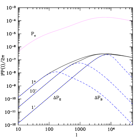
Figure 1: Statistical signal due to multiplicative shear errors. Shown are systematic-error contributions to the power spectra in E mode, $\Delta P_{E}(l)$, (solid) and B mode, $\Delta P_{B}(l)$, (dashed). The correlation function $\xi^{\epsilon}$ of the multiplicative calibration field is assumed to be gaussian with $4\%$ rms. The three plotted power spectra assume different characteristic scales $R_{1/2}$: $1^{\circ}$, $10^{\prime}$ and $1^{\prime}$. At large scales, E mode and B mode contributions are equal to each other for a given characteristic scale. Also shown is the convergence power spectrum $P_{\kappa}(l)$ (dotted).

In fig. 1 we show the power spectrum contributions due to an inhomogeneous calibration field described by the Gaussian correlation function (12) for three characteristic scales $R_{1/2}$: 1^∘, 10^′, and 1^′. We take the rms of the systematics field to be $\Sigma=4\%$. Recall that $\Delta P_{E,B}(l)\propto\Sigma^{2}$. We notice that $\Delta P_{E}$ spectra are featureless and have maxima near the maximum $P_{\kappa}(l)$ (except for very small $R_{1/2}$). On the other hand, the B-mode power spectra $\Delta P_{B}$ have maxima near the characteristic scale of the correlation function.

In order to assess whether the signal due to systematics can be potentially harmful for weak lensing results, let us compare the contaminating power spectra $\Delta P_{E,B}(l)$ to the statistical errors on the convergence power spectrum $\delta P_{\kappa}(l)$ (Kaiser, 1998). Assuming gaussianity of the convergence field we have with sufficient accuracy for our purpose that

$$\delta P_{\kappa}(l)=\frac{1}{\left({l\,\Delta lf_{\mathrm{sky}}}\right)^{1/2}}\,P_{\kappa}(l)\left(1+\frac{\sigma^{2}_{\gamma}}{n_{g}P_{\kappa}(l)}\right),$$ (25)

where $f_{\mathrm{sky}}$ is the fraction of the sky covered by a survey, $n_{g}$ is the density of source galaxies with measured shapes, and $\sigma_{\gamma}\approx 0.3$ is galaxy shape noise. The $P_{\kappa}(l)$ data will have to be binned over some interval $\Delta l$ for a meaningful comparison with the systematic error $\Delta P_{E,B}(l)$. Because $P_{\kappa}(l)$ is virtually featureless and there is no cosmological information in its detailed structure, we choose broad bins of width $\Delta l=l$. An even broader binning scheme would lower the $\delta P_{\kappa}(l)$ line in Figure 2 and our derived requirements on $\Sigma$ would scale as $(\Delta l)^{-1/2}$. Future, ground based, wide-field surveys like LSST are expected to cover $f_{\mathrm{sky}}\sim 50\%$ of the sky and obtain good shape measurements for about $30$ galaxies per $\mathrm{arcmin}^{2}$. Figure 2 shows the convergence power spectrum $P_{\kappa}(l)$ and its statistical errors (25) for these values of $f_{\mathrm{sky}}$ and $n_{g}$. The encouraging implication of fig. 2 is that keeping systematics (e.g, shear calibration errors) below $3\%$ rms ($\Sigma\lesssim 3\%$) should avoid significant contamination of the observed $P_{\kappa}(l)$, even for future surveys.

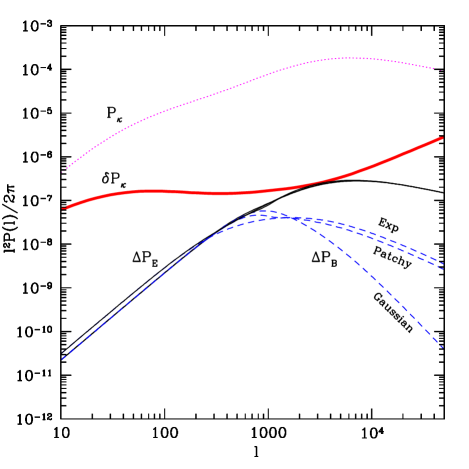
Figure 2: Statistical and systematic errors in the convergence power spectrum $P_{\kappa}(l)$ (dotted): the statistical uncertainties $\delta P_{\kappa}(l)$ are due to sample variance and source galaxy shape noise (thick solid). The systematic uncertainties in E mode, $\Delta P_{E}(l)$, (thin solid) and B mode, $\Delta P_{B}(l)$, (dashed) are shown for different calibration correlation models: Gaussian, “patchy” and exponential. They all share a characteristic scale $R_{1/2}=10^{\prime}$ and $\Sigma=4\%$ rms amplitude. Note that the E-mode systematic errors are essentially independent of the functional form, and are at worst equal to the statistical errors.

Figure 2 plots systematic-error power spectra $\Delta P_{E,B}(l)$ for a gaussian (12), “patchy” (19), and exponential (23) correlation functions, each with $R_{1/2}=10^{\prime}$ and $\Sigma=4\%$. We notice that the shape of $\Delta P_{E,B}(l)$ is nearly independent of the specific shape of the correlation function $\epsilon(\bm{\theta})$ of the systematic field. Thus from a practical point of view the important features of the systematic field are the characteristic scale of correlations and the rms of the field. The latter affects the overall amplitude of the systematic errors as $\Delta P_{E,B}(l)\propto\Sigma^{2}$. The former fixes the amplitude of the $\Delta P_{E}(l)=\Delta P_{B}(l)$ at large scales, and gives the scale where the B mode starts decaying.

We can compare our analytic results for the “patchy” correlation function to the numerical tests of Vale et al. (2004). We set $\theta_{0}=25^{\prime}$ and $\Sigma=10\%$ to match the calibration-error pattern they superpose on their ray-tracing data. Our analytic estimates of the errors induced in the aperture mass variances $\left<M_{{\rm ap},\times}^{2}\right>(R)$ are shown in fig. 3. These errors can be directly compared to those shown in Figure 2 of Vale et al. (2004), which we reproduce in our Figure. Our estimates closely reproduce the results of the numerical simulation, except that we do not produce trough of $\Delta\left<M_{{\rm ap}}^{2}\right>$ at the characteristic scale around $25\,\mathrm{arcmin}$. The trough might be attributable to sample variance from the finite number (64) of patches used in the simulated images.

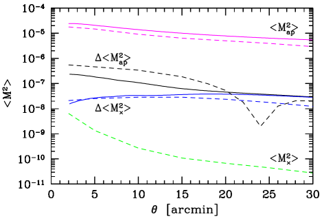
Figure 3: Aperture mass variances as computed analytically in this work (solid) and obtained from ray tracing simulations (Vale et al., 2004) (dashed): there is a good agreement between these two approaches. The two upper curves, denoted by $\left<M_{{\rm ap}}^{2}\right>$ represent the signal from the cosmological E mode (without systematics) and the lowest curve, $\left<M_{{\times}}^{2}\right>$, shows the cosmological contribution to B mode from simulations (in our case this contribution is zero). The two pairs of curves denoted $\Delta\left<M_{{\rm ap}}^{2}\right>$ and $\Delta\left<M_{{\times}}^{2}\right>$ show the systematic signal contribution to the aperture mass variance in E mode and B mode, respectively. The underlying modulation is of “patchy” type with $\theta_{0}=25^{\prime}$ and $10\%$ rms (sec. IV.2).

VI Conclusions

We consider the effect of spatially varying multiplicative systematic errors (assumed uncorrelated with the cosmological signal) on the measured power spectra $P_{E}(l)$ and $P_{B}(l)$ in the case of the 2D lensing. The prime example of this type of systematic would be shear calibration errors which vary across the survey area due to changing observing conditions. As shown by Hirata and Seljak (2003) overall shear calibration errors of existing methods of shear measurement can reach $10\%$ for galaxies of size comparable to the PSF. Such errors grow larger if one uses more poorly-resolved galaxies, as would be the case for deep ground-based surveys like LSST. Uncorrected Galactic extinction could also introduce spatially correlated systematics in survey depth, altering the observed shear correlation functions. When we examine a variety of functional forms for the correlation function $\xi^{\epsilon}$ of the inhomogeneous systematic, we find that all salient effects on the measured power spectrum can be characterized by the variance $\Sigma^{2}$ of the correlation and its characteristic scale $R_{1/2}$. A wide variety of functional forms for $\xi^{\epsilon}$ induced very similar effects on measurements of the convergence power spectrum. Only the small-scale B-mode spectrum is sensitive to the detailed shape of $\xi^{\epsilon}$.

Comparison of the systematics errors $\Delta P_{E}(l)$ on the power spectrum to the statistical errors expected for future weak lensing surveys indicates that we should not be afraid of systematic contamination if we keep calibration errors below $\Sigma\approx 3\%$.

The absence of B-mode contamination in the most recent cosmic-shear measurements (Van Waerbeke et al., 2005; Jarvis and Jain, 2004; Mandelbaum et al., 2005) suggests that systematic errors of the type considered here are below current statistical errors (5–10%) and hence do not bias the conclusions. Note, however, that B-mode power $\Delta P_{B}(l)$ consistent with zero on scales $l\gg 1/\theta_{0}$ does not necessarily imply the absence of significant calibration error $\Delta P_{E}(l)$ (see Figure  1). Hence the present cosmic shear results could be significantly affected by calibration errors, if they have a correlation length $\theta_{0}$ that is larger than scales considered in the B-mode measurement ($\theta_{0}\gg 1/l$). Future surveys will beat down statistical errors, so we will have to understand and beat down systematic errors as well. This work suggests that spatially-varying calibration errors will have to be reduced to 3%. This is well below the levels that have been demonstrated to date, but is probably achievable for well-behaved data with careful shape-measurement techniques (Heymans et al., 2005; Nakajima and Bernstein, 2005).