An Active Instance-based Machine Learning method for Stellar Population Studies

Abstract

We have developed a method for fast and accurate stellar population parameters determination in order to apply it to high resolution galaxy spectra. The method is based on an optimization technique that combines active learning with an instance-based machine learning algorithm.

We tested the method with the retrieval of the star-formation history and dust content in “synthetic” galaxies with a wide range of S/N ratios. The “synthetic” galaxies where constructed using two different grids of high resolution theoretical population synthesis models.

The results of our controlled experiment shows that our method can estimate with good speed and accuracy the parameters of the stellar populations that make up the galaxy even for very low S/N input. For a spectrum with S/N$=5$ the typical average deviation between the input and fitted spectrum is less than $10^{-5}$. Additional improvements are achieved using prior knowledge.

1 Introduction

The availability of large astronomical spectroscopic surveys with moderate spectral resolution such as the 2dF (Colless et al.  2001) or the Sloan Digital Sky Survey (SDSS, York et al. 2000; Stoughton et al. 2002), has prompted the computation of new grids of high resolution spectral synthesis models creating the need of highly efficient methods for the determination of intrinsic physical parameters of a large number of galaxies. There are three intrinsic galactic parameters that are particularly important for studies of cosmological evolution: The star formation and chemical composition histories and the mass distribution of their stellar populations. The importance of the accurate knowledge of these parameters for cosmological studies and for the understanding of galaxy formation and evolution cannot be overestimated. Template fitting has been widely used to carry out estimates of the distribution of age and metallicity from spectral data. Although this technique achieves good results, it is expensive in terms of computing time (therefore is best applied to relatively small samples e.g. Mayya et al. 2004) and the results are in general compromised by the low signal-to-noise data (Kauffmann et al. 2003; Tremonti et al. 2004; Cid fernandes et al. 2005).

Until recently, synthesis models provided either low resolution and a range of metallicities using theoretical atmospheres, or medium resolution at basically solar abundance with the use of empirical stellar spectra. A major problem with theoretical atmospheres used to be that the sampling was coarser than the line broadening observed even in the most massive galaxies. For massive ellipticals with velocity dispersion of up to 400 km s^-1sampling about or better than 7 Å px^-1 in the optical region is needed for representing their spectra with minimum loss of information. For dwarf galaxies or globular clusters with velocity dispersion all the way down to 5-10 km s^-1the optimum sampling is around 0.1 Å px^-1.

Clearly comparing data obtained with sampling of 70 km s^-1 like the SDSS with models with sampling of 1200 km s^-1 at 5000Å  is not satisfactory in the sense that much information associated with atomic lines and even relatively narrow molecular bands will be washed out by the large under sampling. On the other hand, by smoothing or filtering the high frequencies in the data, a more compact and easier/faster to process data set is created (Heavens, Jiménez and Lahav 2000, Heavens et al. 2004).

To overcome these problems we have explored new methods that, while exploiting the high resolution achieved by recent synthesis models, maximize both speed and accuracy in the determination of stellar population parameters.

Minimum distance methods and the closely related chi-square minimization present two significant drawbacks as classification tools. Firstly, they depend crucially on the choice of standard objects to be used; in many problems, it is impossible to select a representative member for each class or each combination of parameters. Secondly, it is difficult to include information regarding intra-class variability, as the only information provided is a typical representative member of the class. Machine learning approaches, on the other hand, use training data that include many representative examples for each class, which makes the selection of standards unnecessary and provides information to determine the features that discriminate members of different classes.

Machine learning algorithms have been shown to significantly outperform minimum distance methods and chi-square minimization in a number of astronomical applications, including stellar classification and determination of stellar atmospheric parameters. For instance, Bailer-Jones (1996) showed that a committee of simple feedforward neural networks yields an error reduction of about 50 percent compared with minimum distance when applied to the task of stellar classification; similar results were reported in Gulati and Gupta (1997). Bailer-Jones (1996) also mentions the fact that, for regions where training data are sparse, the performance advantage of neural network decreases. Thus, methods that automatically add training data to undersampled regions, as the one we present in this paper, are highly desirable.

In this, the first paper of a series, we test a technique that approximates non-linear multidimensional functions using a small initial training set, and by using active learning it increases this training set as needed according to the elements of the test set. This method has shown to outperform traditional instance-base learning algorithms on the problem of interferogram analysis (Fuentes and Solorio, 2004).

Here we present the results of a series of controlled experiments showing that this method can quickly and accurately retrieve the physical parameters of “simulated” galaxies, even at a very low S/N level. Our method takes also advantage of prior domain knowledge which is used to further increase the accuracy of the results obtained. In a forthcoming paper (Solorio et al., in preparation) we apply this methodology to large data sets of galaxy spectra to characterize their stellar population fabric.

2 Testing the method with Synthetic galaxies

Before blindly applying a new method to real data it is reasonable to critically test the procedure in a controlled environment. A crucial aspect is that the validity of the test increases as the test conditions approach the real case. For this reason we have created synthetic galaxies as realistic as possible and necessary in this first step in our research. We thus have applied our methods to a reference set of “synthetic” high resolution spectra of galaxies. To minimize systematics associated with the use of a particular model we have used two different sets of new high resolution spectral synthesis models (for this test only solar metallicity ones) to generate the reference synthetic galaxy spectra set (Bertone et al. 2004: Padova models; González-Delgado et al. 2005: Granada models). The high spectral resolution of the models, allows to use them in the study of narrow absorption lines and for the spectral evolution of the intense line profiles over a wide range of ages. It should be emphasized that our goal is to test the effectiveness of the method in two different sets of models, in order to assess its robustness. We are not trying to determine the respective merits of the models, thus our experiments do not give evidence of any of this. We will address this point in a forthcoming paper.

The Granada models are Single Stellar Population (SSP) synthesis calculated for ages ranging from 1 Myr to 17 Gyr using the Padova and Geneva stellar evolutionary tracks, and their own stellar atmospheres library with spectral sampling of 0.3 Å, and a wavelength coverage of 3000-7000 Å (Martins et al. 2005) . Of the various models available regarding metallicities, we only use for this first work the solar metallicity ones. The synthetic stellar library has been computed with the latest stellar atmospheres, non-LTE for the hot and LTE line-blanketed models for the cold stars. A full description of the models is given by González-Delgado et al. 2005.

A second set of integrated high resolution spectra that we will call the Padova set, was kindly computed for us by A. Bressan (private communication) according to the prescriptions outlined in Bressan, Chiosi and Fagotto (1994). Spectral fluxes along the Bertelli et al. (1994) isochrones were integrated adopting a Salpeter initial mass function (IMF) between 0.15 and 120 $M_{\odot}$. Kurucz high resolution (R=50000) synthetic stellar spectra from 3500Å to 4500Å, were kindly provided by L. Rodríguez, M. Chávez and E. Bertone before publication (Rodríguez-Merino et al. 2005). The red end of the spectra was completed using their 20 Å resolution models from 4500 to 7000 Å (Bressan et al. 1994). The spectral resolution of the SSPs where finally degraded to R=10000.

2.1 Synthetic galaxies

To construct the spectrum of the synthetic galaxies we combined three different populations corresponding to young, intermediate age and old single-age stellar populations (SSP) in varying proportions. To each population we added independent dust attenuation (extinction). The effects of adding noise are discussed in the next section.

Let $f(\lambda)$ be the energy flux emitted by a star or group of stars at wavelength $\lambda$. The flux detected by a measuring device is then $d(\lambda)=f(\lambda)(1-e^{-r\lambda})$, where $r$ is a constant that defines the amount of reddening in the observed spectrum and depends on the size and density of the dust particles in the interstellar medium.

A synthetic galactic spectrum, $g(\lambda)$, can be built given $c_{1},c_{2},c_{3}$, the relative contributions of young, intermediate age and old stellar populations, respectively, their reddening parameters $r_{1},r_{2},r_{3}$, and the ages of the populations $a_{1},a_{2},a_{3}$.

$$g(\lambda)=\sum_{i=1}^{3}c_{i}s(a_{i},\lambda)(1-e^{-r_{i}\lambda})$$ (1)

where $g(\lambda)$ is the energy flux detected at wavelength $\lambda$ and $s(a_{i},\lambda)$ is the flux emitted by a stellar population of age $a_{i}$ at wavelength $\lambda$.

The task of analyzing an observed galaxy spectrum $t$ consists of finding the parameter vector $q=[c_{1},c_{2},c_{3},r_{1},r_{2},r_{3},a_{1},a_{2},a_{3}]$ that minimizeS:

$${\it error}(q)=\sum_{\lambda}(t(\lambda)-g(\lambda))^{2}$$ (2)

Clearly, $c_{1},...,c_{3}$ have to be non-negative, and sum up to 1, also, realistic values of $r_{1},...,r_{3}$ are in the narrow range $[1\times 10^{-5},6\times 10^{-4}]$, and using only a few discrete values for $a_{1},a_{2}$ and $a_{3}$ normally suffices for a reasonable approximation. In particular, for our experiments we consider stellar population ages $a_{1}\in\{3\times 10^{6}\}$, $a_{2}\in\{10^{8},3\times 10^{8},5\times 10^{8},8\times 10^{8}\}$, and $a_{3}\in\{10^{9},2\times 10^{9},3\times 10^{9},5\times 10^{9},10^{10}\}$.

3 The Method

 

0. Let $T$ be the test spectra
1. $S=\{\}$
2. For $i=1$ to n
	2.1. Generate random parameter vector $p=[c_{1},c_{2},c_{3},r_{1},r_{2},r_{3},$
$a_{1},a_{2},a_{3}]$
	2.2. Generate spectra $s$ according to $p$
	2.3. $S=S\cup\{\langle\langle s\rangle,\langle r_{1},r_{2},r_{3}\rangle\rangle$}
3. While $T\neq\{\}$ do:
	3.1. Build $C$, an ensemble of approximators using learning
		algorithm LWLR and training data $S$
	3.2. For every test spectra $t\in T$
		3.2.1. Use $C$ to predict the reddening parameters $r_{1},r_{2},r_{3}$ of $t$
		3.2.2. error($q^{*}$) = $\infty$
		3.2.3. For every triple $\langle a_{1},a_{2},a_{3}\rangle\in\{3\times 10^{6}\}\times\{10^{8},3\times 10^{8},$
$5\times 10^{8},8\times 10^{8}\}\times$ $\{10^{9},2\times 10^{9},3\times 10^{9},5\times 10^{9},10^{10}\}$
			$R=\left[\begin{array}[]{c}s(a_{1},\lambda_{1})(1-e^{-r_{1}\lambda_{1}}),...,s(a_{1},\lambda_{m})(1-e^{-r_{1}\lambda_{m}})\\ s(a_{2},\lambda_{1})(1-e^{-r_{2}\lambda_{1}}),...,s(a_{2},\lambda_{m})(1-e^{-r_{2}\lambda_{m}})\\ s(a_{3},\lambda_{1})(1-e^{-r_{3}\lambda_{1}}),...,s(a_{3},\lambda_{m})(1-e^{-r_{3}\lambda_{m}})\\ \end{array}\right]$
			$[c_{1},c_{2},c_{3}]=t(R^{T}R)^{-1}R^{T}$
			Generate spectra $g$ according to $q=[c_{1},c_{2},c_{3},r_{1},r_{2},r_{3},$
$a_{1},a_{2},a_{3}]$
			error($q$) = $\sum_{\lambda}(g(\lambda)-t(\lambda))^{2}$
			If error($q)<$ error $(q^{*})$
				$q^{*}=q$
				$g^{*}=g$
		3.2.4. If error$(q^{*})<$threshold
			output $\langle t,q^{*}\rangle$
			$T=T-\{t\}$
			Else $S=S\cup\{\langle\langle g^{*}\rangle,\langle r_{1},r_{2},r_{3}\rangle\rangle$}

 

Table 1: Pseudo-code of our Active Learning Algorithm (described in Section 3).

In the application proposed here, galactic spectral analysis, the algorithm estimates the ages of three SSP, their individual contribution to the total light plus the reddening from a high resolution or equivalently high dimensionality input spectrum. In general, all learning algorithms, such as neural networks, C4.5 (Quinlan 1993), and locally weighted regression, face the well known curse of dimensionality (Bellman 1957), which essentially states that the number of training examples needed to approximate a function accurately grows exponentially with the dimensionality of the task. To circumvent the curse of dimensionality, we partition the problem into three subproblems, each of which is amenable to be solved by a different method. The key point is that the dust extinction is a non-linear effect that takes long to estimate, thus if the values of the reddening parameters were known, it would be possible to just perform a search over the possible combinations of values for the ages of stellar populations (a total of $1\times 4\times 5$ = 20 for the Granada models, and a total of 16 for the Padova models), and for each combination of ages find the contributions that best fit the observation using least squares. Then the best overall fit would be the combination of ages and contributions that resulted in the best match to the test spectrum. Thus, the crucial sub-problem to be solved is that of determining the reddening parameters.

Predicting the reddening parameters from spectra is a difficult non-linear optimization problem, specially for the case of noisy spectra. We propose to solve it using an iterative active learning algorithm that learns the function from spectra to reddening parameters. In each iteration, the algorithm uses its training set to build an approximator to predict the reddening parameters of the spectra in the test set. Once the algorithm has predicted these parameters, it uses them to find the combination of ages and contributions that yield the best match to the observed spectra. ¿From these parameters we can generate the corresponding spectrum, and compare it with the spectrum under analysis, if they are a close match, then the parameters found by the algorithm are correct, if not, we can add the newly generated training example (the predicted parameters and their corresponding spectrum) to the training set and proceed to a new iteration. Since this type of active learning adds to the training set examples that are progressively closer to the points of interest, the errors are guaranteed to decrease in every iteration until convergence is attained. In this algorithm the criteria to halt the iterative process can be an error threshold, or a maximum number of iterative steps.

An outline, in the form of pseudocode, of the algorithm is given in table 1. In steps 1 and 2 we build an initial training set $S$ containing $N$ spectra (the attributes), generated for randomly chosen parameter vectors (the target function), applying equation 1. Step 3 forms the main loop, in which we will attempt to obtain the parameters that best match the spectra under analysis (set $T$), this step is repeated until a satisfactory fit has been found for every spectrum in the test set. First, in step 3.1, an approximator $C$ is built using $S$ and an ensemble and locally weighted linear regression (LWLR), a well-known instance-based learning algorithm (Atkeson et al. 1997). Using $C$, we obtain candidate reddening parameters $[r_{1},r_{2},r_{3}]$ for each spectrum in the test set $T$, this is the non-linear part of the problem (step 3.2.1). Given the candidate reddening parameters, in step 3.2.3 we find the ages of the stellar populations $[a_{1},a_{2},a_{3}]$ and their relative contributions $[c_{1},c_{2},c_{3}]$ using a combination of exhaustive search and least squares fitting. For each of the possible 20 combinations of ages we find the relative contributions that best match the spectrum under analysis using a pseudo-inverse computation and then choose among the 20 combination of ages and corresponding contributions the one that minimizes the residuals (equation 2). In step 3.2.4 we simply test if the parameter vector results in a satisfactory fit, if the error for the best approximation, computed as depicted in equation 2, is smaller than a set threshold, it outputs the set of parameters found for that spectrum and removes it from the test set, if the error is not small enough, it adds the new training example to the training set and continues the process.

It should be pointed out that the active learning algorithm is independent of the choice of base learning algorithm used to predict the reddening parameters. Any algorithm that is suitable to predict real-valued target functions from real-valued attributes could be used. In this work we use an ensemble of locally-weighted linear regression (LWLR), but others such as K-nearest-neighbours could have been applied. In the following two sections we briefly present the ideas behind our chosen base learning algorithm.

3.1 Ensembles

An ensemble of classifiers is a set of classifiers whose individual decisions are combined in some way, normally by voting. In order for an ensemble to work properly, individual members of the ensemble need to have uncorrelated errors and an accuracy higher than random guessing. There are several methods for building ensembles. One of them, which is called bagging (Breiman 1996), consists of manipulating the training set. In this technique, each member of the ensemble has a training set consisting of m examples selected randomly with replacement from the original training set of m examples (Dietterich 2000). Another technique similar to bagging manipulates the attribute set. Here, each member of the ensemble uses a different subset randomly chosen from the attribute set. More information concerning ensemble methods, such as boosting and error-correcting output coding, can be found in (Dietterich 2000). The technique used for building an ensemble is chosen according to the learning algorithm used, which in turn is determined by the learning task. In the work presented here, we use the technique that randomly selects subsets of attributes.

3.2 Locally-Weighted Regression

Locally-Weighted Regression (LWR) belongs to the family of instance-based learning algorithms, which includes algorithms as the basic K-nearest neighbour and radial basis functions (Powell 1987). In contrast to most other learning algorithms, which use their training examples to construct explicit global representations of the target function, instance-based learning algorithms simply store some or all of the training examples and postpone any generalization effort until a new instance must be classified. They can thus build query-specific local models, which attempt to fit the training examples only in a region around the query point. In this work we use a linear model around the query point to approximate the target function.

Given a query point ${\bf x_{q}}$, to predict its output parameters ${\bf y_{q}}$, we find the $k$ examples in the training set that are closest to it, and assign to each of them a weight given by the inverse of its distance to the query point: $w_{i}=\frac{1}{|{\bf x_{q}}-{\bf x_{i}}|}$. Let $W$, the weight matrix, be a diagonal matrix with entries $w_{1},\dots,w_{n}$. Let $X$ be a matrix whose rows are the vectors ${\bf x_{1}},\dots,{\bf x_{k}}$, the input parameters of the examples in the training set that are closest to ${\bf x_{q}}$, with the addition of a “1” in the last column. Let $Y$ be a matrix whose rows are the vectors ${\bf y_{1}},\dots,{\bf y_{k}}$, the output parameters of these examples. Then the weighted training data are given by $Z=WX$ and the weighted target function is $V=WY$. Then we use the estimator for the target function ${\bf y_{q}}={\bf x_{q}}^{T}(Z^{T}Z)^{-1}Z^{T}V.$

Thus, locally weighted linear regression is very similar to least-squares linear regression, except that the error terms used to derive the best linear approximation are weighted by the inverse of their distance to the query point. Intuitively, this yields much more accurate results than standard linear regression because the assumption that the target function is linear does not hold in general, but is a good approximation when only a small size neighborhood is considered.

4 Discussion

In all the experiments reported here we used the following procedure: firstly we generated a random set of 200 galactic spectra with their corresponding parameters. This set was then randomly divided into two disjoint subsets, one subset consisting of 50 galactic spectra was used for training and the remaining 150 was considered the test set. This procedure was repeated 10 times, and we report here the overall mean results.

In the first set of experiments our objective was to determine empirically the differences between the active learning procedure versus a traditional ensemble of LWLR. As mentioned previously, the ensembles were constructed selecting randomly a subset of the attributes. To make the comparison objective, both methods used the same attribute subset and an ensemble of size 5. In Figure 1 we show the distribution for prediction errors in intermediate and old ages using the Granada models. This error is measured as the distance in logarithmic steps between the real age and the predicted one. We can see that even though the traditional ensemble of LWLR performs well, our active algorithm achieves higher accuracy. Figure 2 shows error distributions corresponding to the prediction of relative contributions: $c_{1}$,$c_{2}$ and $c_{3}$, of each age population for the Granada models also. We can see that for the active algorithm the central bars are higher than those of an ensemble of LWLR. Error distributions for prediction of reddening parameters are shown in Figure 3. Comparable results in all the experiments were obtained using the Padova models, in Tables 3, 4 and 5 we present the more discrepant results.

Figures 4 and 5 show graphical comparisons between a test spectrum, a reconstructed spectrum using traditional LWLR and our active learning technique for both models. The residuals are always smaller than 3 percent for the LWLR method and clearly much smaller for the active learning technique. The fact that the active learning technique outperformed the traditional ensemble of LWLR was not surprising. Although both are based on the same learning algorithm, LWLR, the training sets from which the predictions are computed are different. The main difference between these two techniques lies on the iterative process of the active learning algorithm. In each iteration, the active learning algorithm augments its training set with new examples that will allow it to better approximate the observed spectra. And this iterative process continues until a suitable solution is found for each spectrum in the test set. As the traditional ensemble of LWLR lacks this iterative process, it will output the best predictions it can reach using only the original training set.

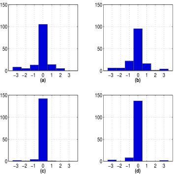
Figure 1: Distribution of errors in the age prediction of intermediate and old populations using the Granada models. Error in age prediction is measured as the distance in logarithmic steps between the age of the test spectrum and the predicted age. Figure (a), intermediate age, and (b), old, are the predictions of a traditional LWLR ensemble. Figures (c) and (d) are the predictions of our algorithm for the same ages and test spectra.

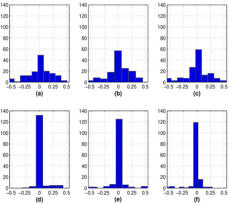
Figure 2: Distribution of prediction errors in the relative contribution parameters $c_{1}$,$c_{2}$, and $c_{3}$ (see section 2.1), using the Granada models. Figures (a) to (c) are the predictions using an ensemble of LWLR for young, intermediate and old populations; figures (d) to (f) are predictions using our active learning algorithm.

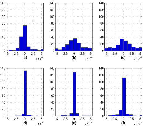
Figure 3: Distribution of prediction errors in the reddening parameters $r_{1}$, $r_{2}$ and $r_{3}$, (see section 2.1), using the Granada models. Figures (a) to (c) are the predictions for young, intermediate and old populations using an ensemble of LWLR, figures (d) to (f) are predictions using our active learning algorithm.

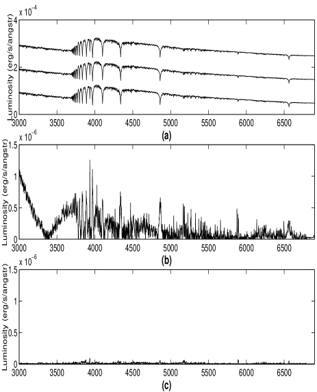
Figure 4: Graphical comparison of results using the Granada models. Figure (a) from top to bottom and shifted by a constant to aid visualization: original test spectrum, spectrum recovered using ensemble of LWLR and spectrum recovered using active learning. Figures (b) and (c) show, in the same scale, the residuals between test and predicted spectra in the same listed order.

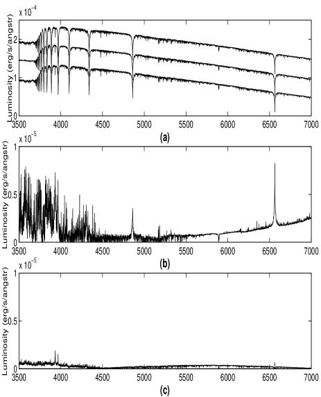
Figure 5: Same as Figure 4 but using the Padova models. Figure (a) from top to bottom and shifted by a constant to aid visualization: original test spectrum, spectrum recovered using ensemble of LWLR and spectrum recovered using active learning. Figures (b) and (c) show, in the same scale, the residuals between test spectrum and predicted spectra in the same listed order. The red end of the spectra was completed using Padova 20 Å resolution models from 4500 to 7000 Å (Bressan et al. 1994).

4.1 The effect of noise

The results presented above are very encouraging. However, the data used in those experiments were noise free. We are aware that noisy data pose a more realistic evaluation of our algorithm, given that in real data analysis noise is always present. Astronomical spectral analysis is no exception to this rule. For this reason, we have performed a set of experiments aimed at exploring the noise-sensitivity of our active learning algorithm. We performed the same procedure described previously, except that this time we added to the test data a Gaussian noise with zero mean and standard deviation of one. We experimented with three different signal to noise (S/N) ratios: 5, 30 and 100 corresponding to bad, normal and good data respectively. Here we present only results for the lower S/N level, given that as the noise level decreases error predictions are more similar to noiseless data experiments.

As a first stage in the treatment of noisy data we used a procedure involving standard principal component analysis (PCA). PCA seeks a set of $M$ orthogonal vectors $v$ and their associated eigenvalues $k$ which best describe the distribution of the data. This module takes as input the training set, and finds its principal components (PC). The noisy test data are projected onto the space defined by the first 20 PC, which were found to account for about 99% of the variance in the set, and the magnitudes of these projections are used as attributes for the algorithm. Experiments with larger number of PC (up to 150) showed no significant improvement in the results.

Figure 6 shows the error distribution in the age prediction using noisy data ($S/N=30$) with an ensemble of LWLR and active learning using the Granada models. In the case of intermediate age prediction, both algorithms achieve almost identical errors. In contrast, for prediction of old populations the active learning algorithm slightly outperforms the ensemble of LWLR. It is important to note that the central peak contains more than 60% of the results, while the +1, -1 bins include about 20% of the cases. For our method, about 85% shows an error in the age determination that is equal or smaller than one age step. Prediction of the relative contributions, presented in Figure 7, is not as peaked as the age prediction but still a substantial fraction is inside a small error. Our method in this case shows a moderate improvement with respect to the LWLR. This same behavior can be observed in Figure 8 where error distribution in the prediction of reddening parameters $r_{1}$,$r_{2}$ and $r_{3}$ are presented. Results for the Padova theoretical models are similar to those for the Granada models, although the improvement achieved by our active learning technique is much higher in the case of the Padova models, specially for the parameters of the old populations. Another set of figures presents results of experiments with very noisy data, using an S/N=5. For the Granada models distribution of errors in predictions are shown in Figures 9, 10 and 11. It is remarkable that even with low quality (S/N=5) data the algorithm does such a good estimate of the population ages. For our method in about 80% of the cases the error in the age determination is equal or less than one age step. However, it is evident that the active technique was unable to improve accuracy due to high levels of noise in some particular cases. For instance, for the Granada models prediction of reddening parameter for young populations, $r_{1}$, presented higher error rates using our algorithm than using a traditional LWLR ensemble. However, in the estimation of reddening for intermediate and old populations the inverse of this occurred, the traditional approach was outperformed by our algorithm. Our algorithm also achieved higher accuracy for the estimation of relative contribution parameters. For the Padova models, in the majority of the cases better results were achieved by the active algorithm; only in one case, the age prediction of old populations, the active algorithm had slightly higher errors. In Figures 12 and 13 we show graphical comparisons between test spectra and reconstructed ones using an LWLR ensemble and our active learning algorithm with an S/N=5. Comparing these figures with the results obtained for noiseless data we can say that the improvement in the fitting of the active technique is lower with very noisy data, although the advantage of the technique is still significant at the lowest S/N ratio.

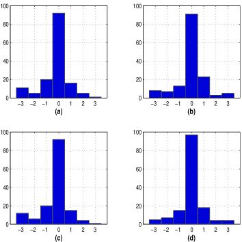
Figure 6: Distribution of errors in the age prediction of intermediate and old populations using the Granada models and an S/N=30. Error in age prediction is measured as the distance in logarithmic steps between the age of the test spectrum and the predicted age. Figure (a), intermediate age, and (b), old, are the predictions of a traditional LWLR ensemble. Figures (c) and (d) are the predictions of our algorithm for the same ages and test spectra.

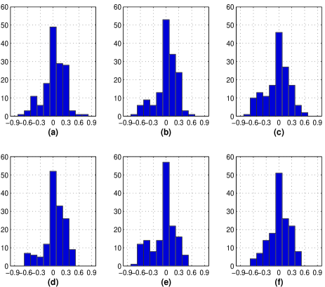
Figure 7: Distribution of prediction errors in the relative contribution parameters $c_{1}$, $c_{2}$ and $c_{3}$ (see section 2.1) using the Granada models and an S/N=30. Figures (a) to (c) are the predictions using an ensemble of LWLR for young, intermediate and old populations; figures (d) to (f) are predictions using our active learning algorithm.

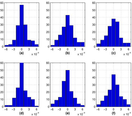
Figure 8: Distribution of prediction errors in the reddening parameters $r_{1}$, $r_{2}$ and $r_{3}$ (see section 2.1) using the Granada models and an S/N=30. Figures (a) to (c) are the predictions using an ensemble of LWLR for young, intermediate and old populations; figures (d) to (f) are predictions using our active learning algorithm.

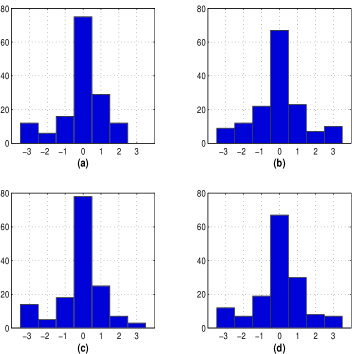
Figure 9: Distribution of errors in the age prediction of intermediate and old populations using the Granada models and an S/N=5. Figure (a), intermediate age, and (b), old, are the predictions of a traditional LWLR ensemble. Figures (c) and (d) are the predictions of our algorithm for the same ages and test spectra.

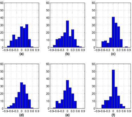
Figure 10: Distribution of errors in the prediction of the relative contribution parameters $c_{1}$, $c_{2}$ and $c_{3}$ (see section 2.1) using the Granada models and an S/N=5. Figures (a) to (c) are the predictions using an ensemble of LWLR for young, intermediate and old populations; figures (d) to (f) are predictions using our active learning algorithm.

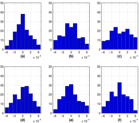
Figure 11: Distribution of prediction errors in the reddening parameters $r_{1}$, $r_{2}$ and $r_{3}$ (see section 2.1) using the Granada models and an S/N=5. Figures (a) to (c) are the predictions using an ensemble of LWLR for young, intermediate and old populations; figures (d) to (f) are predictions using our active learning algorithm.

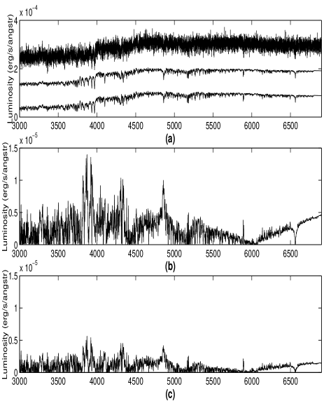
Figure 12: Graphical comparison of results using the Granada models and noisy data, ration S/N=5. Figure (a) from top to bottom and shifted by a constant to aid visualization: noisy test spectrum, spectrum recovered using ensemble of LWLR and spectrum recovered using active learning. Figure (b) show the residuals of the reconstructed spectrum using ensemble of LWLR and figure (c) is the corresponding residuals of using the active learning technique.

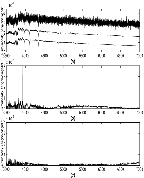
Figure 13: Same as Figure 12 but using the Padova models and noisy data, ratio S/N=5. Figure (a) from top to bottom and shifted by a constant to aid visualization: noisy test spectrum, spectrum recovered using ensemble of LWLR and spectrum recovered using active learning. Figure (b) show the residuals of the reconstructed spectrum using ensemble of LWLR and figure (c) is the corresponding residuals of using the active learning technique.

4.2 Lick Indices

Figure 14: Residuals between a test and a predicted spectrum, the horizontal bands above the residuals show the Lick Indices. We split the spectrum to aid visualization, the top of the figure shows residuals in the blue part while the bottom shows the red part residuals.

One remarkable aspect found in the experiments with noise included is that even when using a large number of PC the residuals showed relatively high peaks in some specific narrow spectral regions. Surprisingly several of these high residual regions coincide with the central band of the Lick indices (listed in Table 2), see Figure 14 where the Lick indices are superimposed on the residuals of the reconstructed spectrum. In other words, giving equal weights to all pixels (or fluxes) produced larger residuals located in these narrow regions.

We opted to explore whether prior knowledge about the Lick indices can help machine learning algorithms to provide a more accurate prediction. Thus, we experimented using two different approaches aimed at giving more influence to the central bands of the Lick indices. In the first approach we discarded all information about most of the spectra, keeping only the flux information corresponding to the central bands of the Lick indices. The learning algorithm thus predicts the reddening parameters using only this reduced subset of fluxes. In a similar way, the contribution of ages is estimated using the same subset of fluxes. Figures 15, 16 and 17 show a comparison of error distributions between active learning when using the original data and active learning when using the Lick indices for the Granada models. We present here only the results using very noisy data (S/N =5) given that previous experiments showed higher error rates for this scenario. For the Padova models using this prior knowledge did not yield higher accuracy in the case of an LWLR ensemble; predictions from active learning using the original data are more accurate. However, when using the Lick indices and active learning reddening parameters are estimated better, as well as the relative contribution of ages. In the case of the Granada models the best results were achieved by active learning using the original data.

Name Index Begin Index End B&H_CNB 3810.0 3910.0 HKratioK 3920.0 3945.0 HKratioH 3955.0 3980.0 Hd 4080.0 4120.0 Lick_CN1 4143.375 4178.375 B&H_CaI 4215.0 4245.0 Lick_Ca4227 4223.500 4236.000 Lick_G4300 4282.625 4317.625 B&H_G 4285.0 4315.0 Hg 4320.0 4360.0 Lick_Fe4383 4370.375 4421.625 Lick_Ca4455 4453.375 4475.875 Lick_Fe4531 4515.500 4560.500 Lick_C4668 4635.250 4721.500 B&H_Hb 4830.0 4890.0 Lick_Hb 4848.875 4877.625 Lick_Fe5015 4979.000 5055.250 Lick_Mg2 5155.375 5197.875 Lick_Fe527 5247.375 5287.375 Lick_Fe5335 5314.125 5354.125 Lick_Fe5406 5390.250 5417.750 Lick_Fe5709 5698.375 5722.125 Lick_Fe5782 5778.375 5798.375 Lick_NaD 5878.625 5911.125 Lick_TiO1 5938.875 5995.875 Lick_TiO2 6191.375 6273.875 Ha 6540.0 6585.0

Table 2: The table was constructed based in the SLOANE index list. We remove the duplicate indices leaving where possible the Lick indices. We also added indices for the Balmer lines, the H$\alpha$, H$\gamma$  and H$\delta$. The HK ratio index was decomposed into two bands. By Index here we mean only the central band and not the continuum side bands.

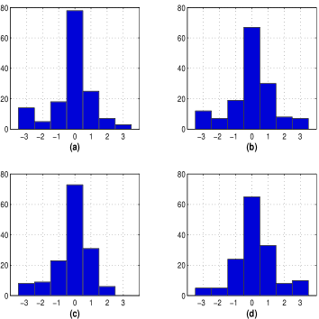
Figure 15: Distribution of errors in the age prediction of intermediate and old populations for the Granada models using an S/N=5. Figure (a), intermediate age, and (b), old, are the predictions of active learning and the original data. Figures (c) and (d) are the predictions of active learning using only the fluxes of the central lines of the Lick indices.

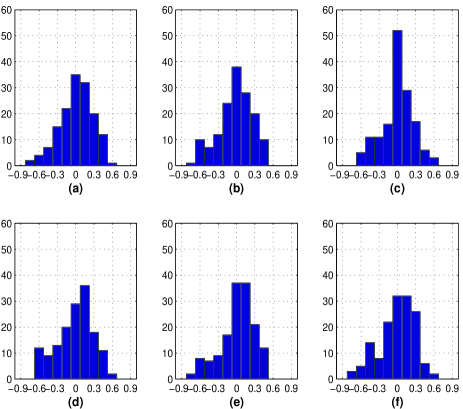
Figure 16: Distribution of prediction errors in the relative contribution parameters $c_{1}$, $c_{2}$ and $c_{3}$ (see section 2.1) for the Granada models using an S/N=5. Figures (a) to (c) are the predictions of active learning and the original data for young, intermediate and old populations respectively. Figures (d) and (f) are the predictions of active learning using only the fluxes of the central lines of the Lick indices.

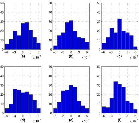
Figure 17: Distribution of prediction errors in the reddening parameters $r_{1}$, $r_{2}$ and $r_{3}$ (see section 2.1) for the Granada models using an S/N=5. Figures (a) to (c) are the predictions of active learning and the original data for young, intermediate and old populations respectively. Figures (d) and (f) are the predictions of active learning using only the fluxes of the central lines of the Lick indices.

The other approach for incorporating prior knowledge consists of increasing the relevance of the Lick indices. By doing so, differences in the Lick indices of the data will have more weight than the differences through the rest of the spectrum; this will be reflected when LWLR selects the closest examples to the test spectrum (see Subsection 3.2). To do this we multiplied the energy fluxes in the wavelengths corresponding to the Lick indices by a constant $k$. That is, fluxes in regions defined by Lick indices where deemed to be $k$ times more important than pixels in other regions. This value of $k=4$ was set experimentally with a 10-fold cross-validation procedure. We present results using very noisy data (S/N=5). These results are similar to results previously discussed. We find that while for the Padova models the best results come from active learning with prior knowledge, for the Granada models this is not the case and the best results come from active learning and the original data. Figures 18 to 20 present error distribution of these experiments. This whole topic will be further investigated in a forthcoming paper, where the method is applied to real data.

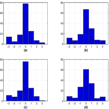
Figure 18: Distribution of prediction errors in the age prediction of intermediate and old populations for the Granada models using an S/N=5. Figure (a), intermediate age, and (b), old, are the predictions of active learning and the original data. Figures (c) and (d) are the predictions of active learning with the fluxes of the central lines of the Lick indices magnified by a constant $k=4$.

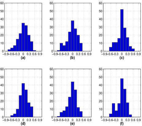
Figure 19: Distribution of prediction errors in the relative contribution parameters $c_{1}$, $c_{2}$ and $c_{3}$ (see section 2.1) for the Granada models using an S/N=5. Figures (a) to (c) are the predictions of active learning and the original data for young, intermediate and old populations respectively. Figures (d) and (f) are the predictions of active learning with the fluxes of the central lines of the Lick indices magnified by a constant $k=4$.

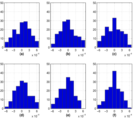
Figure 20: Distribution of prediction errors in the reddening parameters $r_{1}$, $r_{2}$ and $r_{3}$ (see section 2.1) for the Granada models using an S/N=5. Figures (a) to (c) are the predictions of active learning and the original data for young, intermediate and old populations respectively. Figures (d) and (f) are the predictions of active learning with the fluxes of the central lines of the Lick indices magnified by a constant $k=4$.

Using prior knowledge did not yield meaningful improvements, moreover, for some parameters the error increased when incorporating prior knowledge. In another attempt to improve results with very noisy data we carried out another set of experiments. This time we build an ensemble using the predictions from the three approaches: active learning using the original data, active learning using the fluxes corresponding to the Lick indices and active learning with more weight given to fluxes around the central bands of the Lick indices. All the ensemble predictions are then computed as the average of the predictions from each approach.

These results were the most accurate ones, even with high levels of noise, they are presented in Figures 21 to 23. These figures show a marginal improvement with respect to those of Figures 9 to 11. A graphical comparison is presented in Figures 24 and 25. It may be argued that the inclusion of constant Gaussian noise to the synthetic spectrum will produce a low S/N in those regions with lower signal and this will preferentially affect the Lick indices. While some of this is present for the deepest features, it cannot be a major effect for the large majority of the Lick indices where the flux in the control band only changes by less than 20 percent in average with respect to the side bands. The improvement in the concentration of results is clearly illustrated in Table 4 where the central bin frequency increases substantially by the inclusion of prior knowledge. In general, the results obtained from both, the Padova and the Granada models, support the conclusion that the best method when dealing with low S/N data seems to be the combination of ensemble and Prior knowledge.

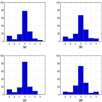
Figure 21: Distribution of prediction errors in the age prediction of intermediate and old populations for the Granada models using an S/N=5. Figure (a), intermediate age, and (b), old, are the predictions of the active learning algorithm. Figures (c) and (d) are the predictions of the ensemble combining prior knowledge.

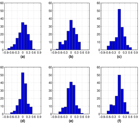
Figure 22: Distribution of prediction errors in the relative contribution parameters $c_{1}$, $c_{2}$ and $c_{3}$ (see section 2.1) for the Granada models using an S/N=5. Figures (a) to (c) are the predictions of active learning and the original data for young, intermediate and old populations respectively. Figures (d) and (f) are the predictions of the active learning ensemble combining prior knowledge.

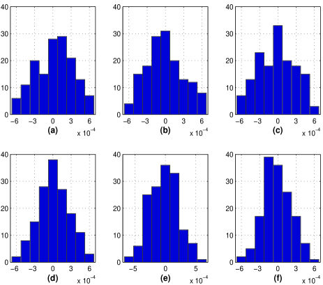
Figure 23: Distribution of prediction errors in the reddening parameters $r_{1}$, $r_{2}$ and $r_{3}$ (see section 2.1) for the Granada models using an S/N=5. Figures (a) to (c) are the predictions of active learning and the original data for young, intermediate and old populations respectively, figures (d) to (f) are predictions of the ensemble combining prior knowledge.

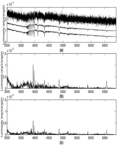
Figure 24: Graphical comparison of results using the Granada models and noisy data, ratio S/N=5. Figure (a) from top to bottom and shifted by a constant to aid visualization: noisy test spectrum, spectrum recovered using active learning and the original data and spectrum recovered using active learning combining predictions. Figures (b) and (c) show the relative difference between test spectrum and predicted spectra in the same listed order.

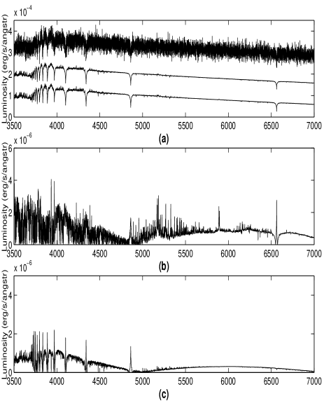
Figure 25: Graphical comparison of results using the Padova models and noisy data, ratio S/N=5. Figure (a) from top to bottom and shifted by a constant to aid visualization: noisy test spectrum, spectrum recovered using active learning and the original data and spectrum recovered using active learning combining predictions. Figures (b) and (c) show the relative difference between test spectrum and predicted spectra in the same listed order.

Results are similar for both sets of theoretical models. However, we can point some interesting differences in the experimental results. For instance, when using noiseless data the method achieves slightly higher prediction accuracies for the Granada models. Another difference mentioned previously is that for the Granada models prior knowledge does not seem to be very useful by itself. Although, the only method that for this models yields better results than active learning with original data, is the combination of the three predictions: original data plus the two methods for using prior knowledge. In contrast, for the Padova models both methods for using prior knowledge improved prediction accuracy. It should be emphasized that these differences between the models are not significative, and we do not consider they can be thought of as evidence of the correctness of the models, but as the relation the spectrum has to the set of parameters on each model. Results on both models show that the ensemble of classifiers combining different forms of incorporating prior knowledge is the best alternative, specially when the data have high levels of noise.

		Bin Centres/Frequencies
Algorithm	Age	-3	-2	-1	0	1	2	3
LWLR ensamble	Intermediate Population	0	15	28	88	15	4	0
	Old Population	8	10	15	46	31	24	16
Active Learning	Intermediate Population	7	13	22	95	11	2	0
	Old Population	7	6	18	42	27	26	24
Ensemble & Prior knowledge	Intermediate Population	4	15	18	99	10	4	0
	Old Populations	4	7	18	55	26	26	14

Table 3: Frequency Table for prediction of ages using the Padova models and an S/N=5.

		Bin Centres/Frequencies
Algorithm	Age	-0.9	-0.75	-0.6	-0.45	-0.3	-0.15	0	0.15	0.3	0.45	0.6	0.75	0.9
LWLR ensamble	Young Population	1	4	10	13	10	13	27	23	30	15	3	0	1
	Intermediate Population	1	1	4	7	16	23	27	34	27	9	1	0	0
	Old Population	0	0	7	13	13	31	31	22	22	9	2	0	0
Active Learning	Young Population	0	3	6	7	11	18	35	36	22	10	2	0	0
	Intermediate Population	1	0	8	8	11	21	36	36	22	7	0	0	0
	Old Population	0	0	5	12	11	22	45	27	19	8	1	0	0
Ensemble & Prior knowledge	Young Population	0	0	3	6	19	28	49	28	14	2	1	0	0
	Intermediate Populations	1	0	2	6	7	33	51	30	15	5	0	0	0
	Old Populations	0	0	1	4	6	23	63	33	17	3	0	0	0

Table 4: Frequency Table for prediction of relative contributions using the Padova models and an S/N=5.

		Bin Centres/Frequencies
Algorithm	Age	-0.0006	-0.00045	-0.0003	-0.00015	0	0.00015	0.0003	0.00045	0.0006
LWLR ensamble	Young Population	12	8	22	24	23	20	16	16	9
	Intermediate Population	11	19	12	28	21	19	18	13	9
	Old Population	14	19	19	19	16	18	14	22	9
Active Learning	Young Population	3	9	21	23	24	23	28	15	4
	Intermediate Population	7	14	21	27	27	21	17	11	5
	Old Population	6	11	19	28	37	23	12	9	5
Ensemble & Prior knowledge	Young Population	1	10	14	23	47	29	19	6	1
	Intermediate Populations	0	5	29	19	43	29	16	6	3
	Old Populations	2	7	16	30	39	26	24	5	1

Table 5: Frequency Table for prediction of reddening parameters using the Padova models and an S/N=5.

5 Conclusions

We presented in this work an optimization algorithm that can estimate with high accuracy: age distributions and mixtures plus the reddening of stellar population in galaxies. The algorithm achieves convergence by iteratively creating new data points that lie in the vicinity of the query point.

Our experimental results using two sets of theoretical models and different levels of noise, show that even with low quality (S/N=5) data the algorithm does a good estimate of the population ages, proportions and reddening. For our method in about 80% of the cases the error in the age determination is equal or less than one age step. In general, the results obtained from both the Padova and the Granada models support the conclusion that the best method when dealing with low S/N data seems to be the combination of an ensemble and prior knowledge. Another important feature of this method is its high speed, it takes $\sim$10 seconds in a normal PC to estimate the parameters of a single 20,000 pixel spectrum. This represents a great advantage over other more conventional methods proposed for this problem, which may take up to a couple of hours to find the solution for such a spectrum.

We will continue our efforts to improve parameter estimation of stellar populations. In forthcoming papers we experiment with models of different metallicities, by adapting this method successfully to this problem. Also, we explore different methods for exploiting prior knowledge and apply them to large spectral databases (e.g. SDSS).

Based on this experimental evaluation we conclude that this method can be applied with similar success to “real” galaxies, reducing the computational cost and thus providing the capability of analyzing large quantities of astronomical spectroscopic data.

References

- Atkeson (1997) Atkeson C.G., Moore A.W., Schaal S., 1997, Artificial Intelligence Review, 11, 11-73
- Bailer-Jones (1996) Bailer-Jones C., 1996, PhD thesis, University of Cambridge
- Bellman (1957) Bellman R. E.,1957, Princeton University Press
- Bertelli (1994) Bertelli, G., Bressan, A., Chiosi, C., Fagotto, F., Nasi, E., 1994, AAS, 106, 275
- Bertone (2004) Bertone, E., Buzzoni, A., Chávez, M., Rodríguez-Merino, L.H., 2004, A.J., 128, 829
- Breiman (1996) Breiman L., 1996, Machine Learning, 24(2):123–140
- Bressan (1994) Bressan A., Chiosi C., Fagotto F., 1994, ApJS, 94, 63
- Cid (2005) Cid Fernandes R., Mateus A., Sodré L., Stasińska G., Gomes J. M., 2005, MNRAS, 358, 363
- Colless (2001) Colless M.M., Dalton G.B., Maddox S.J., Sutherland W.J., Norberg P., Cole S.M., Bland-Hawthorn J., Bridges T.J., Cannon R.D., Collins C.A., Couch W.J., Cross N., Deeley K., De Propris R., Driver S.P., Efstathiou G., Ellis R.S., Frenk C.S., Glazebrook K., Jackson C.A., Lahav O., Lewis I.J., Lumsden S., Madgwick D.S., Peacock J.A., Peterson B.A., Price I.A., Seaborne M., Taylor K., 2001, MNRAS, 328, 1039
- Dietterich (2000) Dietterich T., 2000, In J. Kittler and F. Roli (Ed.), Springer Verlag, 1–15
- Fuentes (2004) Fuentes O., Solorio T., 2004, MICAI 2004, 242–251
- Gonzalez-Delgado (2005) González-Delgado, R.M., Cerviño, M., Martins, L.P., Leitherer, C., Hauschildt, P.H., 2005, MNRAS, 357, 945
- Gulati (1997) Gulati R.K., Gupta R., 1997, Publications of the Astronomical Society of the Pacific, 109, 737, 843–847
- Heavens (2000) Heavens A.F., Jiménez, R., Lahav, O., 2000, MNRAS, 317, 965
- Heavens (2004) Heavens A.F., Panter, B., Jiménez, R., Dunlop, J., 2004, Nature, 428, 625
- Kauffmann (2003) Kauffmann G. et al., 2003, MNRAS, 346, 1055
- Kurucz (1993) Kurucz R. L., 1993, CD-ROM13: Atlas9, SAO,Harvard, Cambridge
- Martins (2005) Martins L.P., González-Delgado R.M., Leitherer C., Cerviño M., Hauschildt P., 2005, MNRAS, 358, 49
- Mayya (2004) Mayya, Y.D., Bressan, A., Rodríguez, M., Valdés, J.R., Chávez, M., 2004, ApJ., 600, 188
- Powell (1987) Powell, M.J.D., 1987, Algorithms for approximation, Oxford: Clarendon Press, 143–167
- Quinlan (1993) Quinlan, J.R., 1993, C4.5 Programs for Machine Learning
- Rodriguez (2005) Rodríguez-Merino L.H., Chavez M., Bertone E., Buzzoni A., 2005, astro-ph/0504307, ApJ, in press
- Stoughton (2002) Stoughton C., Lupton R., Bernardi M., Blanton M., Burles S., Castander F., Connolly A., Eisenstein D., et al., 2002, AJ, 123, 485
- Tremonti (2004) Tremonti C.A., et al. 2004, ApJ, 613, 898
- York (2000) York D.G., et al. 2000, AJ, 120, 1579