A Measurement of the CMB $\left<EE\right>$ Spectrum from the 2003 Flight of Boomerang

Abstract

We report measurements of the CMB polarization power spectra from the January 2003 Antarctic flight of Boomerang. The primary results come from six days of observation of a patch covering 0.22% of the sky centered near $R.A.=82.5^{\circ}$, $Dec=-45^{\circ}$. The observations were made using four pairs of polarization sensitive bolometers operating in bands centered at 145 GHz. Using two independent analysis pipelines, we measure a non-zero $\left<EE\right>$ signal in the range $100<\ell<1000$ with a significance $4.8\sigma$, a $2\sigma$ upper limit of $8.6~{}\mu K^{2}$ for any $\left<BB\right>$ contribution, and a $2\sigma$ upper limit of $7.0~{}\mu K^{2}$ for the $\left<EB\right>$ spectrum. Estimates of foreground intensity fluctuations and the non-detection of $\left<BB\right>$ and $\left<EB\right>$ signals rule out any significant contribution from galactic foregrounds. The results are consistent with a $\Lambda$CDM cosmology seeded by adiabatic perturbations. We note that this is the first detection of CMB polarization with bolometric detectors.

1 Introduction

Measurements of the polarization of the Cosmic Microwave Background (CMB) are a powerful cosmological probe. The CMB is polarized by Thomson scattering (Rees, 1968) during recombination and reionization. Polarization anisotropies have an amplitude which is $\sim 10\%$ of the temperature anisotropies (Bond & Efstathiou, 1984). Similar to CMB temperature anisotropies, the angular power spectra of CMB polarization encode cosmological information. In recent years, CMB temperature anisotropy measurements have provided strong constraints on fundamental cosmological parameters (see e.g. Bond et al. (2003)). The strength of these constraints relies on the assumption that initial perturbations are adiabatic in origin. If an admixture of isocurvature perturbations is allowed, then these constraints are somewhat weakened (Enqvist & Kurki-Suonio, 2000; Bucher et al., 2001). The addition of polarization information can constrain such isocurvature contributions and tighten current constraints derived from temperature anisotropies.

With increased sensitivity, future measurements of CMB polarization will provide new independent constraints on the cosmological model. A measurement of the gravitational lensing of CMB polarization could provide independent constraints on the neutrino mass, the dark energy equation of state and the nature of reionization (Kaplinghat et al., 2003; Hu, 2002). It may also be possible to obtain direct evidence of inflation through its effect on the pattern on CMB polarization (Polnarev, 1985; Crittenden et al., 1993).

Any electromagnetic wave can be described by the Stokes parameters: $I$ is the intensity, $Q$ and $U$ parameterize linear polarization, and $V$ describes the circular polarization. Thomson scattering does not produce circular polarization, so we expect $V=0$ for the CMB. $Q$ and $U$ are not rotationally invariant quantities. Consequently, it is customary to characterize CMB polarization as the sum of curl-free and divergence-free components (Zaldarriaga & Seljak, 1997; Kamionkowski et al., 1997). Using an analogy to electromagnetism, the curl-free components are called E-modes and the divergence free components are called B-modes. E-modes and B-modes are related to $Q$ and $U$ by a non-local linear transformation. There are five observables for CMB polarization: the E-mode correlation function , $\left<EE\right>$, the B-mode correlation function, $\left<BB\right>$, the cross-correlation between E-mode and B-mode polarization, $\left<EB\right>$ and the cross-correlations between temperature anisotropies and polarization, $\left<TE\right>$ and $\left<TB\right>$. All of these correlations are parameterized by multipole moments $C_{\ell}^{XY}$ where $X$ and $Y$ can represent E-modes, B-modes or temperature anistropies.

E-mode polarization of the CMB is primarily produced by scalar fluctuations on the last scattering surface, due to motion of the photon-baryon fluid which is induced by density fluctuations. However, these scalar fluctuations do not produce B-mode polarization on the last scattering surface. Tensor perturbations induced by gravity waves can create CMB polarization as well. Inflationary models generically predict a spectrum of primordial gravity waves which have an amplitude proportional to the fourth power of the energy scale at the time of Inflation (Turner & White, 1996). Gravity waves produce E-mode and B-mode polarization in roughly equal quantities (Seljak & Zaldarriaga, 1997). Given current constraints on tensor perturbations (Seljak et al., 2005), scalar perturbations are expected to dominate the E-mode power spectrum by a factor of at least ten. If parity is preserved in the early universe, then we expect there to be no correlation between E-mode and B-mode polarization (i.e. $\left<EB\right>$ $=0$) or between temperature anisotropies and B-mode polarization ($\left<TB\right>$ $=0$). However, it is possible to construct models where parity is violated and these correlations are non-zero (Pogosian et al., 2002).

In models seeded by purely adiabatic perturbations, acoustic peaks in the E-mode angular power spectrum should be $\sim 180^{\circ}$ out of phase with the acoustic peaks in the temperature anisotropy angular power spectrum, $\left<TT\right>$. Peaks in the E-mode spectrum should line up with troughs in the temperature spectrum, because the scalar component of E-mode polarization is related to velocities and not densities on the last scattering surface. The angular spectrum of the cross-correlation between temperature anisotropies and E-mode polarization ($\left<TE\right>$) will show a series of acoustic peaks which occur between the peaks of the $\left<TT\right>$ and $\left<EE\right>$ power spectra. Measurements of the $\left<EE\right>$ power spectrum by DASI (Kovac et al., 2002; Leitch et al., 2004), CBI (Readhead et al., 2004) and CAPMAP (Barkats et al., 2005) along with $\left<TE\right>$ measurements by DASI, WMAP (Kogut et al., 2003), and CBI provide evidence that the assumption of adiabatic perturbations is valid.

In this paper, we report a measurement of the E-mode polarization power spectrum from the second Antarctic flight of Boomerang which took place in January 2003 (hereafter B03). The telescope and instrument configuration from the 1997 test flight and the first Antarctic flight are discussed in Piacentini et al. (2002) and Crill et al. (2003) respectively. The instrument configuration for the 2003 flight is described in Masi et al. (2005) along with the data processing and the CMB maps. Results for the temperature anisotropy spectrum and the temperature-polarization cross-correlation are reported in Jones et al. (2005a) and Piacentini et al. (2005) respectively. Cosmological parameter constraints are reported in MacTavish et al. (2005). In this paper, we briefly review the instrument and observations in §2. In §3, we discuss the analysis methods used to estimate the polarization power spectra, and in §2 we present the power spectrum results. §5 provides a discussion of systematic errors, and §6 describes tests for foreground contamination.

2 Instrument and Observations

Boomerang is a balloon-borne telescope designed for long duration flights around Antarctica. In its first Antarctic flight (December 1998), Boomerang measured CMB temperature anisotropies using bolometers operating with bands centered at 90, 150, 220 and 410 GHz (Crill et al., 2003; Ruhl et al., 2003). For the 2003 flight, the receiver was re-designed to measure CMB temperature and polarization anisotropies with bands centered at 145, 245 and 345 GHz (Masi et al., 2005). The results reported here come from four pairs of polarization sensitive bolometers (PSB’s) operating at 145 GHz (Jones et al., 2003, 2005b).

Figure 1: Sky coverage from the 2003 Boomerang flight. The top panel shows the large region covered during the first part of the flight (the shallow region) and the bottom panel is the smaller region covered during the second half of the flight (the deep region). In the top panel, the outer set of black lines shows the sky cut used in the shallow mask. The inner outline shows the outline of the deep region sky cut. The shallow scans covered 3.0% of the sky, and sky cut used for the CMB analysis covers 1.8%. The deep region observations covered 0.28% of the sky and the outlined region covering 0.22% of the sky was used for the CMB analysis. The integration time per pixel for the deep observations is roughly 20 times longer than integration time per pixel during shallow observations. In both panels, the small circles represent regions of map which are excised due to the presence of known point sources.

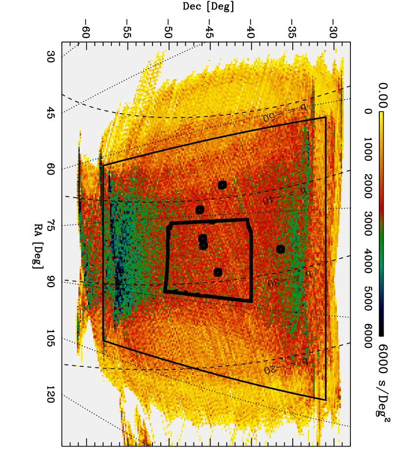
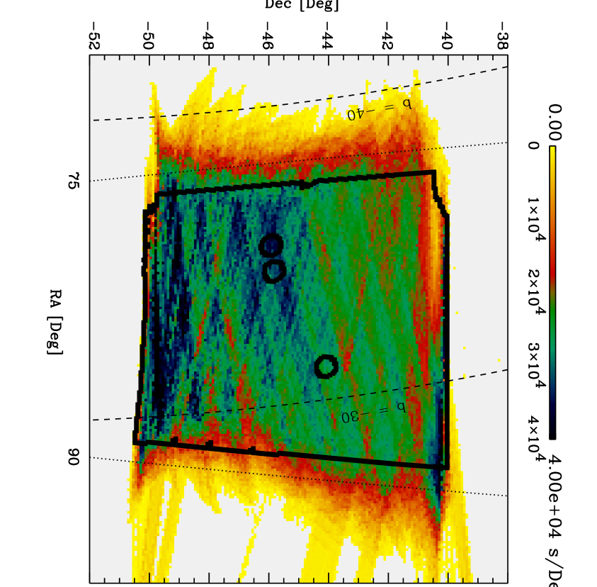
The 2003 flight of Boomerang was launched on January 6, 2003 from McMurdo Station, Antarctica and lasted 14 days. In this paper, we report on the analysis of 205 hours of CMB observations during the first 11 days. During this period 75 hours were spent scanning a large region (called the shallow region) comprising 3.0% of the sky and 125 hours on a small region (called the deep region) comprising 0.28% of the sky. The shallow region was designed to optimally measure the degree scale signals in $\left<TT\right>$ and $\left<TE\right>$, while deep region was designed to optimize the signal-to-noise ratio on the $\left<EE\right>$ and $\left<BB\right>$ and $\left<EB\right>$ power spectra. For these spectra almost all the statistical weight comes from the deep region.

Figure 1 shows the distribution of integration time over the observation region and the sky cuts used in the analysis. The time per pixel in the deep region is a factor of $\sim 20$ longer than in the shallow region. For the spectral analysis, we use 1.8% of the sky for the shallow region and 0.22% of the sky for the deep region. These choices were made so that the coverage was roughly uniform in time per sky pixel and for the different channels in the focal plane. Another consideration was that the deep and shallow observations could each be split in half (in time) and still cover their respective sky cuts (which is useful for systematic tests).

3 Data Analysis Methods

We used two independent pipelines for the map-making and polarization power spectrum estimation. Masi et al. (2005) describes the bulk of the data analysis from raw data to CMB maps including: raw data cleaning, detector characterization, pointing reconstruction, calibration, beam measurement, noise estimation and making polarized maps. In this paper, we limit the discussion to aspects of power spectrum estimation for polarized datasets.

The two pipelines are independent to a high degree. In the following, “NA pipeline” refers to the pipeline primarily based in North America and “IT pipeline” refers to the pipeline developed in Italy. Each team had many choices to make about instrument characteristics and data analysis techniques. The boundaries of the shallow and deep region sky cuts used by both teams are identical, but differences in the data cleaning causes slight differences in integration time. As we will show in the §2, the two pipelines yield compatible answers; this is a testament to the robustness of the data set.

3.1 Power Spectrum Estimation

Both pipelines are polarized extensions of the Monte Carlo based MASTER method (Hivon et al., 2002) first used on B98 (Netterfield et al., 2002). These techniques rely on spherical harmonic transformations done on a partial map of the sky. For polarization data, the Q and U maps are expanded as a function of spin-2 spherical harmonics

$$(Q\pm iU)(\hat{n})=\sum_{lm}(a^{E}_{lm}\pm ia^{B}_{lm})_{\pm 2}Y_{lm}(\hat{n}),$$ (1)

where $a^{E}_{lm}$ and $a^{B}_{lm}$ are the coefficients for E-mode and B-mode polarization respectively. These coefficients can be calculated in a manner similar to Legendre transformations,

$$a^{E}_{lm} =\frac{1}{2}\int d\Omega W(\hat{n})\Big{[}(Q+iU)(\hat{n})_{+2}Y_{lm}(\hat{n})$$

$$+(Q-iU)(\hat{n})_{-2}Y_{lm}(\hat{n})\Big{]},$$ (2)

$$a^{B}_{lm} =\frac{1}{2i}\int d\Omega W(\hat{n})\Big{[}(Q+iU)(\hat{n})_{+2}Y_{lm}(\hat{n})$$

$$-(Q-iU)(\hat{n})_{-2}Y_{lm}(\hat{n})\Big{]},$$ (3)

where $W(\hat{n})$ is an arbitrary weighting function and the integral extends only over the observed portion of the sky. From these transforms, we can build three observables:

$$C_{\ell}^{EE} = \frac{1}{2\ell+1}\sum_{\ell}|a^{E}_{lm}|^{2},$$ (4)

$$C_{\ell}^{BB} = \frac{1}{2\ell+1}\sum_{\ell}|a^{B}_{lm}|^{2},$$ (5)

$$C_{\ell}^{EB} = \frac{1}{2\ell+1}\sum_{\ell}a^{E}_{lm}a^{B*}_{lm},$$ (6)

where $C_{\ell}^{\mathrm{EE}}$ the E-mode power spectrum, $C_{\ell}^{\mathrm{BB}}$ the B-mode power spectrum, and $C_{\ell}^{\mathrm{EB}}$ the cross-correlation between E-mode and B-mode polarization. $C_{\ell}^{\mathrm{EB}}$ is expected to be zero if parity is preserved in the early universe. Our estimates of the cross-correlations between temperature and polarization ($C_{\ell}^{\mathrm{TE}}$ and $C_{\ell}^{\mathrm{TB}}$) are discussed in Piacentini et al. (2005).

For spherical harmonic transforms done on the cut sky the measure of $C_{\ell}$ is biased; we describe them as pseudo-$C_{\ell}$’s ($\widetilde{C}_{\ell}$). For the polarization power spectra, the relationships between full-sky $C_{\ell}$ and $\widetilde{C}_{\ell}$ are expressed as

$$\widetilde{C}_{\ell}^{\mathrm{EE}} =\sum_{\ell^{\prime}}\Big{[}{\vphantom{Y}}_{+}K_{\ell\ell^{\prime}}F_{\ell^{\prime}}^{EE}B_{\ell^{\prime}}^{2}C_{\ell^{\prime}}^{\mathrm{EE}}$$

$$+{\vphantom{Y}}_{-}K_{\ell\ell^{\prime}}F_{\ell^{\prime}}^{BB}B_{\ell^{\prime}}^{2}C_{\ell^{\prime}}^{\mathrm{BB}}\Big{]}+\widetilde{N}_{\ell}^{\mathrm{EE}},$$ (7)

$$\widetilde{C}_{\ell}^{\mathrm{BB}} =\sum_{\ell^{\prime}}\Big{[}{\vphantom{Y}}_{+}K_{\ell\ell^{\prime}}F_{\ell^{\prime}}^{BB}B_{\ell^{\prime}}^{2}C_{\ell^{\prime}}^{\mathrm{BB}}$$

$$+{\vphantom{Y}}_{-}K_{\ell\ell^{\prime}}F_{\ell^{\prime}}^{EE}B_{\ell^{\prime}}^{2}C_{\ell^{\prime}}^{\mathrm{EE}}\Big{]}+\widetilde{N}_{\ell}^{\mathrm{BB}},$$ (8)

$$\widetilde{C}_{\ell}^{\mathrm{EB}} =\sum_{\ell^{\prime}}\Big{[}{\vphantom{Y}}_{+}K_{\ell\ell^{\prime}}-{\vphantom{Y}}_{-}K_{\ell\ell^{\prime}}\Big{]}F_{\ell^{\prime}}^{EB}B_{\ell^{\prime}}^{2}C_{\ell^{\prime}}^{\mathrm{EB}}$$

$$+\widetilde{N}_{\ell}^{\mathrm{EB}},$$ (9)

where $C_{\ell}^{\mathrm{XY}}$ represents the full-sky power spectrum, $B_{\ell}$ is the beam window function, $F_{\ell}^{XY}$ is the transfer function measured by signal-only Monte Carlo simulations, $\widetilde{N}_{\ell}^{\mathrm{XY}}$ is the noise bias measured by noise-only Monte Carlo simulations, ${}_{+}K_{\ell\ell^{\prime}}$ is the primary coupling kernel and ${}_{-}K_{\ell\ell^{\prime}}$ describes the geometric leakage between E-modes and B-modes (Chon et al., 2004). Both pipelines use roughly 500 Monte Carlo simulations of signal-only and noise-only data streams to estimate the signal transfer function and noise bias respectively. A similar number of signal+noise simulations can be used to estimate the uncertainty on the spectral estimate and check for bias in the pipeline.

Since we observe a small portion of the sky, we are not able to measure individual multipole moments. Instead, we parameterize the power spectrum as a piecewise continuous function

$$C_{\ell}^{\mathrm{XY}}=q^{XY}_{b}C_{\ell}^{(S)\mathrm{XY}},$$ (10)

where $q^{XY}_{b}$ is the bandpower deviation over a range $(\Delta\ell)_{b}$ and $C_{\ell}^{(S)\mathrm{XY}}$ is a shape parameter. Common choices for the shape parameter are those that keep $C_{\ell}^{(S)}$ constant over the band, those that keep $\ell(\ell+1)C_{\ell}^{(S)}/(2\pi)$ constant over the band (i.e. the flattened spectrum) or those that represent a theoretically motivated power spectrum (e.g. $\Lambda$CDM concordance model). The choice of parameterization depends in part on the nature of the expected signal and the noise in the maps.

The output bandpower ${\cal C}_{b}^{XY}$ (${\cal C}_{\ell}=\ell(\ell+1)C_{\ell}/2\pi$) is then a function of $q^{XY}_{b}$ and $C_{\ell}^{(S)\mathrm{XY}}$

$${\cal C}_{b}^{XY}=q^{XY}_{b}\frac{\sum_{\ell\in b}\frac{2\ell+1}{4\pi}C_{\ell}^{(S)\mathrm{XY}}}{\sum_{\ell\in b}\frac{\ell+\frac{1}{2}}{\ell(\ell+1)}}$$ (11)

When comparing to a model, the expected bandpower deviation can be written as

$$\left<q_{b}\right>=\frac{{\cal I}[W^{b}_{\ell}{\cal C}_{\ell}]}{{\cal I}[W^{b}_{\ell}{\cal C}_{\ell}^{(S)}]},$$ (12)

where $W^{b}_{\ell}$ is the bandpower window function, ${\cal C}_{\ell}^{(S)}=\ell(\ell+1)C_{\ell}^{(S)}/2\pi$ and ${\cal I}[f_{\ell}]$ is the logarithmic integral (Bond et al., 2000)

$${\cal I}[f_{\ell}]=\sum_{\ell}\frac{\ell+\frac{1}{2}}{\ell(\ell+1)}f_{\ell}.$$ (13)

For general shape functions, we get

$$\left<q_{b}\right>=\frac{{\cal I}[W^{b}_{\ell}{\cal C}_{\ell}]}{{\cal I}[W^{b}_{\ell}{\cal C}_{\ell}^{(S)}]},$$ (14)

and we can recover $\left<{\cal C}_{b}\right>$ using equation 11. If ${\cal C}_{\ell}^{(S)}=$ constant, then we have

$$\left<{\cal C}_{b}\right>=\frac{{\cal I}[{\cal C}_{\ell}W^{b}_{\ell}]}{{\cal I}[W^{b}_{\ell}]}.$$ (15)

3.2 NA Pipeline

For the NA pipeline, a quadratic estimator (Bond et al., 1998) is used to iteratively solve for the bandpowers and their uncertainty. This estimator (called Xfaster) is capable of solving for the power spectra of a single map or any combination of two or more maps (which can be overlapping) while accounting for all correlations between those maps (Contaldi et al., 2005).

For B03, Xfaster is used to solve for the combined power spectrum of the shallow and deep region data (the combined power spectra are called the 2Mask spectra). Separate maps are made from the shallow and deep region observations; this insures that the only correlations between the maps are due to sky signal. When we perform the spherical harmonic transformations, we use a uniform pixel weighting for the shallow map, and pixels in the deep region are weighted by the inverse square root of noise in that pixel ($\sigma_{pix}^{-1/2}$). An effective noise weighting is also applied in the spectrum estimation process due to noise bias of each map ($\widetilde{N}_{\ell}^{\mathrm{XY}}$). This is an efficient way to account for the imbalance of integration time per pixel between the shallow and deep maps.

Although the shallow region does not contribute much statistical weight to the polarization spectra, it does significantly reduce the sample variance in the $\left<TT\right>$ and $\left<TE\right>$ spectra. The Xfaster method is used for the polarization spectra so that we can derive consistent correlation matrices between all spectra for use in parameter estimation (MacTavish et al., 2005).

3.3 IT Pipeline

To solve for the power spectrum, the IT pipeline uses a method similar to that described in Hivon et al. (2002) but adapted for polarization spectra (see e.g. Kogut et al. (2003) and Challinor & Chon (2005)). Errors bars and correlation matrices are calculated using bandpowers resulting from signal+noise Monte Carlo simulations. The IT pipeline performs the $\left<EE\right>$, $\left<BB\right>$ and $\left<EB\right>$ analysis on the deep region maps with the pixels weighted by the inverse square root of the noise ($\sigma_{pix}^{-1/2}$). The IT maps also include data from shallow observations which fall inside the deep region.

3.4 Testing Goodness-of-Fit

To test how well particular models fit our data, we use the standard likelihood ratio technique in a manner similar to recent work done by DASI (Kovac et al., 2002; Leitch et al., 2004) and CBI (Readhead et al., 2004). Specifically, we calculate the logarithm of the ratio of the peak of the likelihood to the likelihood of a model ${\mathcal{M}}$ parametrized by bandpowers ${\cal C}_{b}$:

$$\Lambda({\cal C}_{b})=\ln\left(\frac{L(\overline{{\cal C}}_{b})}{L({\cal C}_{b})}\right),$$ (16)

where $\overline{{\cal C}}_{b}$ are the maximum likelihood bandpowers. The larger this ratio is, the worse the model ${\mathcal{M}}$ fits the data. In this paper, we are primarily concerned with comparisons to the null hypothesis (${\cal C}_{b}=0$ for all $b$) and our fiducial $\Lambda$CDM model (the best fit to the WMAP $\left<TT\right>$ spectra from Spergel et al. (2003)).

In the approximation that the likelihood function $L({\cal C}_{b})$ is a multivariate Gaussian near its peak (which is generally a good approximation when the signal to noise ratio in a band is $\gg 1$), we have $\Lambda=\Delta\chi^{2}/2$. If we assume that a given model ${\mathcal{M}}$ is true, the probability of observing $\Lambda$ exceeding a particular value of is given by the “probability to exceed” ($PTE$)

$$PTE(\Lambda)=\frac{1}{\Gamma(N/2)}\int_{\Lambda}^{\infty}e^{-x}x^{\frac{N}{2}-1}dx,$$ (17)

where $N$ is the number of parameters and $\Gamma(x)$ is the complete gamma function. For example, if $PTE$=5%, then we can reject the hypothesis that the model ${\mathcal{M}}$ is true with 95% confidence.

Since our power spectrum estimators do not calculate full likelihood values, we use the offset log-normal function, $Z_{b}=\ln({\cal C}_{b}+x_{b})$, to approximate the likelihood function (Bond et al., 2000) where ${\cal C}_{b}$ is the bandpower and $x_{b}$ is the offset parameter. The likelihood is calculated by

$$\sigma_{b}= \Delta\overline{{\cal C}}_{b}/(\overline{{\cal C}}_{b}+x_{b})$$ (18)

$$\Delta Z_{b}= \ln({\cal C}_{b}+x_{b})-\ln(\overline{{\cal C}}_{b}+x_{b})$$ (19)

$$-2\ln L({\cal C}_{b})= \sum_{bb^{\prime}}\Delta Z_{b}\sigma_{b}^{-1}G_{bb^{\prime}}\sigma_{b^{\prime}}^{-1}\Delta Z_{b^{\prime}}^{-1}$$ (20)

where $\overline{{\cal C}}_{b}$ is the maximum likelihood bandpower and $G_{bb^{\prime}}$ is the bandpower correlation matrix which is normalized to unity on the diagonals. In this parameterization, the likelihood is normalized to the peak value (i.e. $\ln L(\overline{{\cal C}}_{b})=0$).

In the results to follow, we compute $\Lambda$ and PTE separately for the $\left<EE\right>$, $\left<BB\right>$ and $\left<EB\right>$ spectra. In other words, when performing this test on one spectrum, we marginalize over the other spectra by excising the correlations between spectra from the inverse Fisher matrix.

4 Results

Figure 2: Angular Power Spectra Results. From top to bottom the panels show the $\left<EE\right>$, $\left<BB\right>$ and $\left<EB\right>$ power spectrum results from the NA (blue circles) and IT (red squares) pipelines. The solid line in the $\left<EE\right>$ plot is the best fit $\Lambda$CDM model to the WMAP $\left<TT\right>$ results (Spergel et al., 2003) and the dashed line in all plots represent zero-signal. From these plots and the statistical tests in Table 2, it is clear the $\left<BB\right>$ and $\left<EB\right>$ are consistent with zero signal while $\left<EE\right>$ is consistent with $\Lambda$CDM, but inconsistent with zero signal. The $\Lambda$CDM $\left<EE\right>$ model predicted by the WMAP $\left<TT\right>$ results is nearly identical the best fit $\left<EE\right>$ model predicted from recent $\left<TT\right>$ results including B03 (MacTavish et al., 2005).

4.1 Narrow Band Analysis

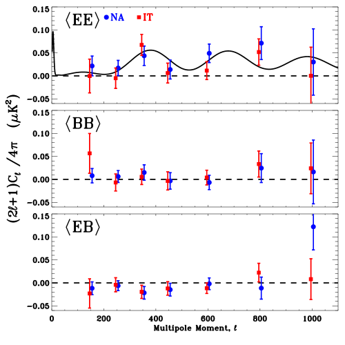
The $\left<EE\right>$, $\left<BB\right>$ and $\left<EB\right>$ power spectra results from both pipelines are shown in Figure 2 and listed in Table 1. The multipole range shown is from $101\leq\ell\leq 1100$; information on scales $2\leq\ell\leq 100$ and $\ell\geq 1101$ is discarded. These data, $x_{b}$’s, window functions and correlation matrices are available at http://cmb.case.edu/boomerang and http://oberon.roma1.infn.it/boomerang.

Although we use a shape function which is constant in $\ell(\ell+1)C_{\ell}/(2\pi)$, we choose to plot the results in terms of $(2\ell+1)C_{\ell}/(4\pi)$ to emphasize our sensitivity in the range $100<\ell<1100$ and relate the power spectrum directly to the r.m.s. CMB signal

$$\sigma_{CMB}^{2}=\sum_{\ell}\frac{2\ell+1}{4\pi}C_{\ell}.$$ (21)

The results from the two pipelines show a high degree of consistency. Additionally, the NA deep-only power spectra are nearly identical to the 2Mask spectra plotted here. Different choices in the data processing (e.g. time domain filtering, the number of map iterations, detector relative calibrations) could lead to the small discrepancy between the NA and IT results.

				NA		IT
	$\ell_{min}$	$\ell_{max}$	$\ell_{center}$	$\overline{{\cal C}}_{b}$	$\Delta\overline{{\cal C}}_{b}$	$\overline{{\cal C}}_{b}$	$\Delta\overline{{\cal C}}_{b}$
$\left<EE\right>$	101	200	150	3.3	3.2	-0.04	5.5
	201	300	250	4.3	4.2	-1.24	5.6
	301	400	350	15.3	7.40	23.7	8.0
	401	500	450	6.3	9.3	2.8	9.7
	501	700	600	29.5	12.1	6.94	11.7
	701	900	800	57.0	28.6	41.6	23.0
	901	1100	1000	30.2	72.1	0.3	62.2
$\left<BB\right>$	101	200	150	1.2	2.4	8.5	6.5
	201	300	250	1.6	3.2	-1.7	4.7
	301	400	350	5.3	5.8	2.0	5.9
	401	500	450	-1.5	8.1	-1.4	8.9
	501	700	600	-4.0	9.3	2.4	9.6
	701	900	800	19.7	25.2	26.7	22.7
	901	1100	1000	16.3	69.4	24.1	55.2
$\left<EB\right>$	101	200	150	-1.8	2.1	-3.5	4.8
	201	300	250	-1.5	2.7	-1.0	3.8
	301	400	350	-7.6	4.8	-6.8	5.0
	401	500	450	-6.6	6.3	-5.4	6.6
	501	700	600	-1.1	7.6	-6.9	6.9
	701	900	800	-9.1	19.1	17.9	16.2
	901	1000	1000	122.1	50.4	8.2	44.3

Table 1: Power spectra results for $\left<EE\right>$, $\left<BB\right>$ and $\left<EB\right>$ from the NA and IT analysis pipelines. The first three columns define the $\ell$-bins used and the next four columns state the bandpowers and errors from both pipelines. $\overline{{\cal C}}_{b}$ and $\Delta\overline{{\cal C}}_{b}$ (${\cal C}_{\ell}=\ell(\ell+1)C_{\ell}/2\pi$) have units $\mu K^{2}$. Power spectra, $x_{b}$’s, window functions and correlation matrices are available at http://cmb.case.edu/boomerang and http://oberon.roma1.infn.it/boomerang.

	Fiducial Model				No Polarization
	NA		IT		NA		IT
	$\Lambda$	PTE	$\Lambda$	PTE	$\Lambda$	PTE	$\Lambda$	PTE
$\left<EE\right>$	2.6	0.63	3.2	0.49	11.8	$1.3\times 10^{-3}$	7.2	0.05
$\left<BB\right>$	6.6	0.07	9.2	0.01	1.3	0.92	2.0	0.78
$\left<EB\right>$	-	-	-	-	5.8	0.11	2.6	0.64

Table 2: Table of values for the $\Lambda$ statistic and “probability to exceed” (PTE) calculated from the narrow band results in Figure 2 and Table 1. We compare $\left<EE\right>$ and $\left<BB\right>$ to the fiducial $\Lambda$CDM model (the best fit to the WMAP $\left<TT\right>$ from Spergel et al. (2003)) and we test the null hypothesis (no polarization signal) on all three spectra. Both data sets are assumed to have 7 degrees of freedom. For both data sets $\left<EE\right>$ is a good fit to fiducial model and inconsistent with the null hypothesis. $\left<BB\right>$ is not a good fit to fiducial model, but is consistent with no signal. $\left<EB\right>$ is consistent with zero signal.

In Figure 2, only the $\left<EE\right>$ spectrum appears to be significantly different from zero. To quantify this, we calculate the $\Lambda$ statistic for the assumption of zero polarized signal. The results in Table 2 show that the $\left<EE\right>$ result is inconsistent with zero signal and that $\left<BB\right>$ and $\left<EB\right>$ are both consistent with zero. Similarly, we compare $\left<EE\right>$ and $\left<BB\right>$ to the E-mode power spectrum from the fiducial $\Lambda$CDM model. In this case, the $\left<EE\right>$ result is in good agreement with the fiducial E-mode spectrum while $\left<BB\right>$ is not. For these calculations, the IT data and the NA $\left<EB\right>$ data are taken to have $x_{b}=0$.

4.2 Wide Band Analysis

To assess the raw significance of our $\left<EE\right>$ result and to set an upper limit for $\left<BB\right>$ and $\left<EB\right>$ spectra, we perform a wide band analysis over a range $201\leq\ell\leq 1000$ (the actual analysis uses three bins with bins defined by $2\leq\ell\leq 200$ and $1001\leq\ell\leq 1999$ used as “junk” bins). We used four different shape functions for the bandpowers: constant in $C_{\ell}$, constant in $(2\ell+1)C_{\ell}/4\pi$, constant in $\ell(\ell+1)C_{\ell}/2\pi$ and the fiducial $\Lambda$CDM model. Sky cuts and spectrum estimation are the same as those used in the narrow band analysis.

			$\left<EE\right>$		$\left<BB\right>$		$\left<EB\right>$
Shape	Pipeline	$\left<{\cal C}_{b}^{EE}\right>$	${\cal C}_{b}$	$\Delta{\cal C}_{b}$	${\cal C}_{b}$	$\Delta{\cal C}_{b}$	${\cal C}_{b}$	$\Delta{\cal C}_{b}$
$\ell(\ell+1)C_{\ell}/(2\pi)$	NA 2mask	9.94	11.5	3.0	2.0	2.2	-4.00	1.9
	IT deep	15.5	14.2	6.3	8.0	5.7	-0.2	3.9
$C_{\ell}$	NA 2mask	19.4	23.4	5.2	3.3	4.3	-4.7	3.5
$(2\ell+1)C_{\ell}/4\pi$	NA 2mask	14.9	17.5	4.0	2.5	3.15	-5.1	2.6
$\Lambda$CDM	NA 2mask	15.4	16.4	3.8	3.3	3.0	-	-

Table 3: Wide band analysis results for $200\leq\ell\leq 1000$. The $Shape$ column refers to the band power parameterization: flat in $\ell(\ell+1)C_{\ell}/(2\pi)$, flat in $C_{\ell}$ and $\Lambda$CDM. The column labeled $\left<{\cal C}_{b}^{EE}\right>$ is the $\left<EE\right>$ expectation value for an ensemble of Monte Carlo simulations using the B03 instrument noise and the fiducial $\Lambda$CDM model as the CMB input. $\left<{\cal C}_{b}^{EE}\right>$, ${\cal C}_{b}$ and $\Delta{\cal C}_{b}$ have units $\mu K^{2}$ and are quoted in terms of $\ell(\ell+1)C_{\ell}/(2\pi)$. $\left<EB\right>$ is not calculated for the $\Lambda$CDM shape, since it can go positive and negative.

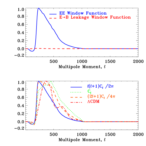
Table 3 shows the bandpower results for all cases of the wide band analysis and Table 4 shows the $\Lambda$ statistic and PTE for each case. In all cases, the $\left<BB\right>$ and $\left<EB\right>$ results are consistent with zero signal while the $\left<EE\right>$ signal is significantly non-zero. The choice of shape function and the fine details of the bandpower estimator have an effect on the output bandpowers. The NA and IT bandpowers agree closely with the results from Monte Carlo simulations of each method using the fiducial $\Lambda$CDM model as the input. When we parameterize the spectra as flat in $\ell(\ell+1)C_{\ell}/(2\pi)$, the simulations also show that the difference in error bars is consistent with the differences between the NA and IT estimators. This difference is illustrated by the top panel of Figure 3 which shows the wide-band window function used by the NA Xfaster estimator. Xfaster performs an effective Wiener filter where most of the statistical weight comes from the lower edge of the band. The IT estimator uses a flat window function which leads to a less optimal result. The bottom panel of Figure 3 shows how the NA window functions varies with the choice of shape function.

For each parameterization, the $\Lambda$ statistic and $PTE$ results from the wide band analysis are reported in Table 4. For a single bandpower, the significance of the detection can be calculated by

$$S=\sqrt{2\Lambda},$$ (22)

where $S$ is the detection significance quoted in units of $\sigma$. With the NA results, we find that the shape function which is constant in $C_{\ell}/2\pi$ produces the highest significance, but its significance is only slightly higher than what we find when using $(2\ell+1)C_{\ell}/4\pi$ or $\Lambda$CDM as the shape function. For the case parametrized as constant in $C_{\ell}$, we find that the $\left<EE\right>$ bandpower is consistent with a $4.8\sigma$ detection. For this same case, we quote $2\sigma$ upper limits of $8.6~{}\mu K^{2}$ for $\left<BB\right>$ and $7.0~{}\mu K^{2}$ for $\left<EB\right>$.

Figure 3: Window functions from the NA wide band results in Tables 3 and 4. In the top panel the solid blue line is the $\left<EE\right>$ window function for the band $201\geq\ell\leq 1000$. The dashed red line characterizes the leakage of E-modes into B-modes ($E\rightarrow B$) which has a maximum value of $\sim 0.01$. The $\left<BB\right>$ window function and $B\rightarrow E$ leakage window function are similar to those plotted here. The low amplitude of the $E\rightarrow B$ and $B\rightarrow E$ shows that B03 is able to separate E-mode and B-mode polarization. In the bottom panel, the window functions are shown for the different power spectrum parameterizations (i.e. $C_{\ell}^{(S)}$) used in the bandpower estimation. The shape of the $\left<EE\right>$ window function indicates the effective weight applied to each multipole moment. For all cases used in the NA analysis, the window function is significantly different than the flat band used in the IT wide band analysis. This is due to an effective Wiener filter which weights each multipole by $C_{\ell}^{(S)}/(C_{\ell}+N_{\ell})^{2}$ where $N_{\ell}$ is the noise at a given multipole, $C_{\ell}^{(S)}$ is the shape function and $C_{\ell}$ is the expected signal. In a given band the expected signal depends on the form of $C_{\ell}^{(S)}$.

		$\left<EE\right>$		$\left<BB\right>$		$\left<EB\right>$
Shape	Mask	$\Lambda$	PTE	$\Lambda$	PTE	$\Lambda$	PTE
$\ell(\ell+1)C_{\ell}/(2\pi)$	NA 2mask	8.6	$3.4\times 10^{-5}$	0.42	0.36	2.2	0.04
	IT deep	2.5	0.02	1.0	0.16	$1.0\times 10^{-3}$	0.97
$C_{\ell}$	NA 2mask	11.4	$1.9\times 10^{-6}$	0.30	0.44	0.94	0.17
$(2\ell+1)C_{\ell}/4\pi$	NA 2mask	10.7	$3.7\times 10^{-6}$	0.32	0.42	1.9	0.05
$\Lambda$CDM	NA 2mask	10.4	$5.3\times 10^{-6}$	0.61	0.27	-	-

Table 4: Values of the $\Lambda$ statistic and the PTE from the comparison of the wide band the bandpowers in Table 3 to a model with zero polarization signal. The $\left<EE\right>$ data is inconsistent with zero, while $\left<BB\right>$ and $\left<EB\right>$ are consistent with no polarization signal.

5 Systematic Errors

Given the small amplitude of the polarization signal, we need tight control on systematic errors. For most systematic errors, we would expect them to contribute equally to $\left<EE\right>$ and $\left<BB\right>$ which could also lead to a non-zero $\left<EB\right>$. The fact that $\left<BB\right>$ and $\left<EB\right>$ are consistent with zero gives credibility to the $\left<EE\right>$ result. To further establish the robustness of our result, we performed two types of internal consistency checks and a suite of Monte Carlo simulations to determine limits on systematic errors due to instrument mis-characterization.

5.1 Internal Consistency Tests

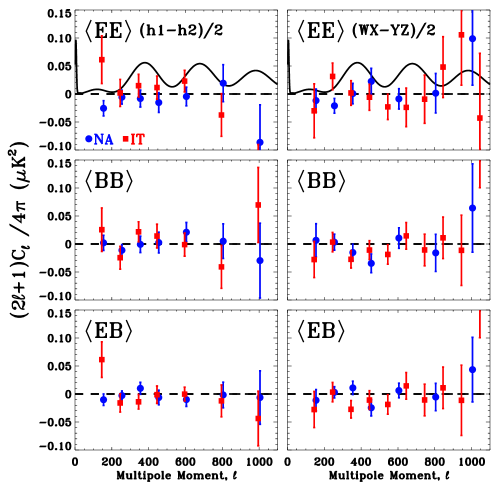
To check the consistency of our result, we performed jackknife tests which are done by splitting the data in half, making maps $\Delta_{1}$ and $\Delta_{2}$ from each half and measuring the power spectrum of $(\Delta_{1}-\Delta_{2})/2$. If this power spectrum is consistent with zero then the dataset is considered to be internally consistent. We performed two sets of jackknife tests. The first test involves splitting the data in time (called the $(h1-h2)/2$ test). The second test is done by comparing detectors on the left and right side of the focal plane (called the (WX-YZ)/2 test). The $(h1-h2)/2$ is sensitive to time-varying systematic problems while the (WX-YZ)/2 is sensitive to problems affecting individual channels.

The mapmaking process for the $(h1-h2)/2$ test is different in the NA and IT pipelines. With the NA pipeline, we make maps from the first and second half of the shallow observations ($\Delta_{h1}^{S}$ and $\Delta_{h2}^{S}$), and first and second half of the deep observations ($\Delta_{h1}^{D}$ and $\Delta_{h2}^{D}$). We then use Xfaster to estimate the combined power spectrum of $(\Delta_{h1}^{S}-\Delta_{h2}^{S})/2$ and $(\Delta_{h1}^{D}-\Delta_{h2}^{D})/2$. With the IT pipeline, we make a combined map from the first half of the shallow observations and the first half of deep observations $\Delta_{h1}^{SD}$. Similarly, $\Delta_{h2}^{SD}$ is made from second halves of the shallow and deep observations. The IT esimator is then used to estimate the power spectrum of $(\Delta_{h1}^{SD}-\Delta_{h2}^{SD})/2$ on the deep region mask.

As discussed in Masi et al. (2005), each side of the focal plane has two PSB pairs at 145 GHz which were oriented so that the left and right sides of the focal plane could measure Stokes $Q$ and $U$ independently. The (WX-YZ)/2 is done by taking the difference of maps made from from the left (WX) and right (YZ) sides of the focal plane. In the same manner used for the $(h1-h2)/2$ test, the NA pipeline makes separate (WX-YZ)/2 maps from the shallow and deep observations while the IT pipeline makes a combined (WX-YZ)/2 map from the deep and shallow data. For each pipeline, the power spectra are estimated in the same way as in the $(h1-h2)/2$ test.

Figure 4 shows the results for the $(h1-h2)/2$ and the (WX-YZ)/2 tests, and Table 5 shows $\chi^{2}$ and PTE’s calculated from those results . For each pipeline, both jackknife tests are consistent with zero for all three spectra. These tests put strong limits on systematic problems.

Figure 4: Results of Jackknife Tests. The left side shows the results for the $(h1-h2)/2$ test and the right side shows the results for the (WX-YZ)/2 test. The blue circles are results from the NA pipeline and the red squares are results from the IT pipeline. Table 5 shows the $\chi^{2}$ and $PTE$ calculated from these results. For both tests, all three spectra are consistent with zero signal.

	NA		IT
Spectrum	$\chi^{2}$	PTE	$\chi^{2}$	PTE
$\left<EE\right>$ $(h1-h2)/2$	6.9	0.44	10.6	0.16
$\left<BB\right>$ $(h1-h2)/2$	3.0	0.89	6.0	0.54
$\left<EB\right>$ $(h1-h2)/2$	3.0	0.89	6.9	0.44
$\left<EE\right>$ (WX-YZ)/2	5.5	0.60	5.9	0.75
$\left<BB\right>$ (WX-YZ)/2	6.7	0.46	1.5	0.997
$\left<EB\right>$ (WX-YZ)/2	5.1	0.65	6.0	0.74

Table 5: Reduced $\chi^{2}$ and “probabilty to exceed” calculated from the jackknife results (Figure 4). Both pipelines have 7 degrees of freedom.

5.2 Simulation of Instrument Characterization Errors

Mis-characterization of instrumental parameters is a potential source of systematic error in the power spectra. The primary parameters of concern are: beam size, calibration, polarization efficiency, detector time constant and polarization angle. An error in beam size leads to a bin-dependent scaling factor. Errors in the absolute calibration and polarization efficiency lead to an overall scaling factor. Errors in relative calibrations or detector time constants lead to leakage of CMB temperature anisotropies into the polarization signal. An error in the polarization angle mixes the $Q$ and $U$ Stokes parameters.

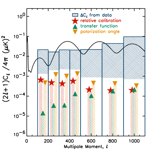
The measurement of B03 instrument parameters is described in Masi et al. (2005) and the uncertainties on those parameters are shown here in Table 6. To estimate the error induced by potential errors in relative calibration, time constant, polarization efficiency and polarization angle, we performed a suite of signal-only Monte Carlo simulations. For each parameter, we performed 145 simulations starting with the same simulated sky map (a realization of the fiducial $\Lambda$CDM model). We then create a time-ordered datastream where the value of the parameter is randomly varied for each detector. The values are drawn from a distribution representing our uncertainty on that parameter. We then analyze this data stream using the measured parameter values. For each Monte Carlo, we estimate the power spectrum using a technique similar to that used by the IT pipeline. We then compute the systematic error bar by taking the standard deviation of Monte Carlo results. Figure 5 shows the results of the simulations. The induced systematic error bars are less than 10% of the bandpower uncertainty. On most scales, the polarization angle is the dominant source of error.

Parameter	Uncertainty	Induced Error on Spectrum
beam FWHM	$0.23^{\prime}$	2.5% at $\ell=500$, 10% at $\ell=1000$
absolute calibration	1.8%	3.6%
polarization efficiency	3%	4%
relative calibration	0.8%	See Figure 5
polarization angle	$2^{\circ}$	See Figure 5
time constant	10%	See Figure 5

Table 6: Instrument parameters, the uncertainty on their characterization and the induced error on the $\left<EE\right>$ power spectrum. Errors in beam size, absolute calibration and polarization efficiency result in a re-scaling of the power spectrum. Errors in relative calibration, polarization angle and time constant are more complicated; see Figure 5 for the induced error bars.

Although uncertainty in the beam size is a relatively benign problem, beam differences between elements in a PSB pair and structure in the cross-polar beam pattern of a given detector could lead to irreducible leakage of temperature anisotropies into the polarization maps. Given the off-axis structure of the Boomerang optics (where the axis of symmetry is vertical), the beam mismatch between elements in a PSB pair depends on the polarization angles of each element. For example, detectors oriented at $45^{\circ}$ and $-45^{\circ}$ with respect to horizon have well matched beams while detectors oriented at $0^{\circ}$ and $90^{\circ}$ will have slightly different beams. A physical optics simulation confirmed that the latter case has the worst mismatch among all four PSB pairs. For this worst case, we calculate the differential beam window function and estimate the leakage of temperature anisotropy into polarization using the fiducial $\Lambda$CDM model. We find this signal to be smaller than our measured $\left<EE\right>$ signal by a factor of $10^{3}$ (or more) on the angular scales that we are sensitive to. This calculation represents the worst case scenario because sky rotation should reduce this contamination somewhat.

Differences between the cross-polar beams in a PSB pair could also lead to temperature anisotropy leakage. The integrated cross-polar beam for a given detector is a factor of $\sim 200$ smaller than the integrated co-polar beam. Here if we take the worst case scenario (i.e. that the throughput of cross-polar beam difference is twice the throughput of the cross-polar beam of one detector), a naive estimate of the $\left<TT\right>$ leakage into $\left<EE\right>$ gives $\left<EE\right>_{leak}\lesssim 10^{-4}$$\left<TT\right>$ which is $\lesssim$ 1% of the observed $\left<EE\right>$.

Figure 5: Propagation of measurement errors in instrumental parameters to $\left<EE\right>$ error. The hatched bands show the upper edges of the $\left<EE\right>$ error (due to noise) for the bands in the multi-bin NA results (Figure 2). The other symbols show errors in relative calibration (stars), bolometer time constant (upward triangles) and polarization angle (downward triangles). Because errors in absolute calibration and polarization efficiency are multiplicative factors which act identically on each bin, their effect is left off this plot and reported instead in Table 6.

6 Foregrounds

Polarized emission from galactic and extra-galactic sources are another potential source of contamination (de Oliveira-Costa, 2004; Tucci et al., 2005). Currently, not much is known about diffuse polarized emission in the frequency range $30<\nu<400$ GHz. Synchrotron emission is expected to be highly polarized, but the power steeply decreases with increasing frequency ($\alpha\sim-3$). Recent observations with the ACTA telescope have detected polarized synchrotron emission in a small patch near the edge of our deep region at frequencies of 1.4 GHz (Bernardi et al., 2003) and 2.3 GHz (Carretti et al., 2005). A naive extrapolation of these synchrotron results to 145 GHz predicts a signal of $0.2~{}\mu K$ r.m.s. compared to a $\sim 3~{}\mu K$ r.m.s. expected from the fiducial $\Lambda$CDM model given our beam.

From starlight polarization measurements (Fosalba et al., 2002), dust is expected to be less than 10% polarized, with a spectral index $\alpha\sim 1.7$, but it could be higher depending on the nature of the galactic magnetic field (Wright, 1987). Results from Archeops (Benoît et al., 2004; Ponthieu et al., 2005) measure a polarization fraction of $5-10\%$ for dust clouds near the galactic plane, but the results are not sensitive enough to place strong limits on degree scale dust polarization away from the galactic plane.

From the 145 GHz data alone, we are highly confident that our E-mode polarization signal is dominated by the CMB and not foreground emission. Foreground emission should produce nearly equal parts E-mode and B-mode polarization. Non-detection of any B-mode signal (Figure 2 and Tables 1-4) strongly implies a lack of foreground polarization. In Piacentini et al. (2005), the B03 $\left<TB\right>$ signal is consistent with zero while $\left<TE\right>$ is consistent with $\Lambda$CDM. Further evidence is obtained by cross-correlating an IRAS dust intensity map with the 145 GHz polarization data. Both the $\left<T_{IRAS}B_{B03}\right>$ and $\left<T_{IRAS}E_{B03}\right>$ are consistent with zero. We find that the consistency of the deep-only and combined shallow+deep power spectra rule out large dust polarization signals in regions nearer to the galactic plane.

In Masi et al. (2005), we characterize the dust emission by comparing the three B03 intensity maps to dust templates from Schlegel et al. (1998). In the deep region, we detect a dust intensity correlation at $2.5\sigma$ with our 345 GHz channels, but find an upper limit of $4~{}\mu K_{CMB}$ r.m.s. for dust intensity at 145 GHz. If we assume that dust is 10% polarized, we get an upper limit of $0.4~{}\mu K_{CMB}$ r.m.s. for the dust polarization signal at 145 GHz. A polarized analysis of 245 and 345 GHz data will be discussed in a future work.

Lastly, the difference of the intensity maps at 145 and 345 GHz shows what appears to be three small regions of diffuse dust emission which appear to be correlated with IRAS emission (see Figure 27 of Masi et al. (2005)). As one final test, we perform a spectrum analysis on a sky cut where we excised square blocks centered on these clouds. The boundaries of the blocks are reported in Table 7. The resulting polarized power spectra are identical to the ones reported here.

R.A. limits		Dec. limits
84∘	85∘	-48.5∘	-47.25∘
87.5∘	88.75∘	-48.5∘	-47.25∘
87.5∘	88.5∘	-49.5∘	-50.5∘

Table 7: Regions of potential dust contamination where found by taking the difference between the B03 145 and 345 GHz intensity maps. The polarization spectra were re-calculated with the data in these regions excised. The resulting spectra are identical to those in Figure 2 and Table 1.

7 Conclusions

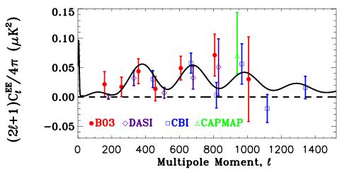
In this paper, we report the measurement of the $\left<EE\right>$  $\left<BB\right>$ and $\left<EB\right>$ polarization power spectra from the 2003 flight of Boomerang. Consistent results have been obtained from two different data analysis pipelines. These results have passed a wide variety of systematic tests and the induced error from instrumental uncertainties is negligible. The $\left<BB\right>$ and $\left<EB\right>$ results are consistent with zero signal, as expected in $\Lambda$CDM models dominated by scalar adiabatic perturbations. The $\left<EE\right>$ results are consistent with existing measurements (Figure 6) and a good fit to the $\left<EE\right>$ signal expected from the $\Lambda$CDM model which is the best fit to the WMAP $\left<TT\right>$ results. Several tests using higher frequency channels and dust maps, in addition to the fact that $\left<BB\right>$ and $\left<EB\right>$ are consistent with zero, argue that it is very unlikely that the $\left<EE\right>$ result is contaminated by galactic emission. This detection of $\left<EE\right>$ is the first by a bolometric polarimeter, and thus bodes well for the future of CMB polarimetry using bolometric detectors.

Figure 6: Comparison of B03 $\left<EE\right>$ results with existing results from DASI Leitch et al. (2004), CBI Readhead et al. (2004) and CAPMAP Barkats et al. (2005). The model is the fiducial $\Lambda$CDM model.

References

- Barkats et al. (2005) Barkats, D. et al. 2005, ApJ, 619, L127
- Benoît et al. (2004) Benoît, A. et al. 2004, A&A, 424, 571
- Bernardi et al. (2003) Bernardi, G., Carretti, E., Cortiglioni, S., Sault, R. J., Kesteven, M. J., & Poppi, S. 2003, ApJ, 594, L5
- Bond et al. (2003) Bond, J. R., Contaldi, C. R., & Pogosyan, D. 2003, Philosophical Transactions Royal Society of London A, 361, 2435
- Bond & Efstathiou (1984) Bond, J. R. & Efstathiou, G. 1984, ApJ, 285, L45
- Bond et al. (1998) Bond, J. R., Jaffe, A. H., & Knox, L. 1998, Phys. Rev. D, 57, 2117
- Bond et al. (2000) —. 2000, ApJ, 533, 19
- Bucher et al. (2001) Bucher, M., Moodley, K., & Turok, N. 2001, Physical Review Letters, 87, 191301
- Carretti et al. (2005) Carretti, E. et al. 2005, submitted to MNRAS, astro-ph/0503043
- Challinor & Chon (2005) Challinor, A. & Chon, G. 2005, MNRAS, 360, 509
- Chon et al. (2004) Chon, G., Challinor, A., Hivon, E., Prunet, S., & Szapudi, I. 2004, MNRAS, 350, 914
- Contaldi et al. (2005) Contaldi, C. R. et al. 2005, in preparation
- Crill et al. (2003) Crill, B. P. et al. 2003, ApJS, 148, 527
- Crittenden et al. (1993) Crittenden, R., Davis, R. L., & Steinhardt, P. J. 1993, ApJ, 417, L13
- de Oliveira-Costa (2004) de Oliveira-Costa, A. 2004, in proceedings of ”Astronomical Polarimetry - Current Status and Future Directions”, Hawaii, USA, March 15-19 2004
- Enqvist & Kurki-Suonio (2000) Enqvist, K. & Kurki-Suonio, H. 2000, Phys. Rev. D, 61, 043002
- Frigo & Johnson (2005) Frigo, M. & Johnson, S. G. 2005, Proceedings of IEEE, 93, 216
- Fosalba et al. (2002) Fosalba, P., Lazarian, A., Prunet, S., & Tauber, J. A. 2002, in AIP Conf. Proc. 609: Astrophysical Polarized Backgrounds, 44–50
- Górski et al. (2005) Górski, K. M., Hivon, E., Banday, A. J., Wandelt, B. D., Hansen, F. K., Reinecke, M., & Bartelmann, M. 2005, ApJ, 622, 759
- Hivon et al. (2002) Hivon, E., Górski, K. M., Netterfield, C. B., Crill, B. P., Prunet, S., & Hansen, F. 2002, ApJ, 567, 2
- Hu (2002) Hu, W. 2002, Phys. Rev. D, 65, 023003
- Jones et al. (2003) Jones, W. C., Bhatia, R. S., Bock, J. J., & Lange, A. E. 2003, in Proceedings of SPIE Vol. 4855 Millimeter and Submillimeter Detectors for Astronomy, edited by T.G. Phillips, J. Zmuidzinas, (SPIE, Bellingham, WA)
- Jones et al. (2005a) Jones, W. C. et al. 2005a, submitted to ApJ
- Jones et al. (2005b) —. 2005b, in preparation
- Kamionkowski et al. (1997) Kamionkowski, M., Kosowsky, A., & Stebbins, A. 1997, Phys. Rev. D, 55, 7368
- Kaplinghat et al. (2003) Kaplinghat, M., Knox, L., & Song, Y.-S. 2003, Phys. Rev. Lett., 91, 241301
- Kogut et al. (2003) Kogut, A. et al. 2003, ApJS, 148, 161
- Kovac et al. (2002) Kovac, J. M., Leitch, E. M., Pryke, C., Carlstrom, J. E., Halverson, N. W., & Holzapfel, W. L. 2002, Nature, 420, 772
- Leitch et al. (2004) Leitch, E. et al. 2004, submitted to ApJ
- MacTavish et al. (2005) MacTavish, C. et al. 2005, submitted to ApJ
- Masi et al. (2005) Masi, S. et al. 2005, submitted to A&A
- Netterfield et al. (2002) Netterfield, C. B. et al. 2002, ApJ, 571, 604
- Piacentini et al. (2002) Piacentini, F. et al. 2002, ApJS, 138, 315
- Piacentini et al. (2005) Piacentini, F. et al. 2005, submitted to ApJ
- Pogosian et al. (2002) Pogosian, L., Vachaspati, T., & Winitzki, S. 2002, Phys. Rev. D, 65, 083502
- Polnarev (1985) Polnarev, A. G. 1985, Soviet Ast., 29, 607
- Ponthieu et al. (2005) Ponthieu, N. et al. 2005, submitted to A&A, astro-ph/0501427
- Readhead et al. (2004) Readhead, A. C. S et al. 2004, Science, 306, 836
- Rees (1968) Rees, M. J. 1968, ApJ, 153, L1
- Ruhl et al. (2003) Ruhl, J. E. et al. 2003, ApJ, 599, 786
- Schlegel et al. (1998) Schlegel, D. J., Finkbeiner, D. P., & Davis, M. 1998, ApJ, 500, 525
- Seljak et al. (2005) Seljak, U. et al. 2005, Phys. Rev. D, 71, 103515
- Seljak & Zaldarriaga (1997) Seljak, U. & Zaldarriaga, M. 1997, Physical Review Letters, 78, 2054
- Spergel et al. (2003) Spergel, D. N. et al. 2003, ApJS, 148, 175
- Tucci et al. (2005) Tucci, M., Martinez-Gonzalez, E., Vielva, P., & Delabrouille, J. 2005, submitted to A&A, astro-ph/0411567
- Turner & White (1996) Turner, M. S. & White, M. 1996, Phys. Rev. D, 53, 6822
- Wright (1987) Wright, E. L. 1987, ApJ, 320, 818
- Zaldarriaga & Seljak (1997) Zaldarriaga, M. & Seljak, U. 1997, Phys. Rev. D, 55, 1830