Measuring the geometry of the Universe in the presence of isocurvature modes

Abstract

The Cosmic Microwave Background (CMB) anisotropy constrains the geometry of the Universe because the positions of the acoustic peaks of the angular power spectrum depend strongly on the curvature of underlying three-dimensional space. In this Letter we exploit current observations to determine the spatial geometry of the Universe in the presence of isocurvature modes. Previous analyses have always assumed that the cosmological perturbations were initially adiabatic. A priori one might expect that allowing additional isocurvature modes would substantially degrade the constraints on the curvature of the Universe. We find, however, that if one considers additional data sets, the geometry remains well constrained. When the most general isocurvature perturbation is allowed, the CMB alone can only poorly constrain the geometry to $\Omega_{0}=1.6\pm 0.3$. Including large-scale structure (LSS) data one obtains $\Omega_{0}=1.07\pm 0.03,$ and $\Omega_{0}=1.06\pm 0.02$ when supplemented by the Hubble Space Telescope (HST) Key Project determination of $H_{0}$ and SNIa data.

One of the most striking successes of observational cosmology over the past few years has been the constraint of possible departures of the geometry of our universe from a spatially flat (Euclidean) geometry. Such a departure from spatial flatness may be characterized by the dimensionless quantity $\Omega_{K},$ related by the Friedmann-Robertson-Walker equations to the fractional energy density (with respect to the critical density) $\Omega_{0}$ of the Universe by the relation $\Omega_{K}=1-\Omega_{0}$. If $\Omega_{K}<0,$ the Universe has a three-dimensional spherical geometry, if $\Omega_{K}>0,$ a hyperbolic geometry, and if $\Omega_{K}=0,$ a Euclidean (flat) geometry. When a structure of a given physical size is viewed from a cosmological distance, its angular size depends sensitively on the spatial geometry. Different spatial geometries yield different laws of perspective. Such differences may be exploited to obtain a measurement of $\Omega_{K}$ using the angular power spectrum of the CMB anisotropy omega_theory . In the standard Big Bang thermal history, the Universe, previously ionized, recombined into neutral atoms at a redshift $z_{rec}\approx 1080.$ At this moment the photon mean free path increased precipitously, and since then the CMB photons have travelled freely toward us with virtually no rescattering. Prior to recombination the previously tightly coupled plasma had undergone acoustic oscillations, manifested in the CMB spectrum today by the so-called Doppler peaks. At recombination these oscillations were characterized by a physical scale $d^{*}_{rec},$ the size of the sound horizon at recombination. In order to convert $d^{*}_{rec}$ into an angular scale $\theta^{*},$ another length scale $d_{AD}$ is required. Let $d_{LS}$ eqn be the diameter of the last scattering surface expressed in terms of present day co-moving units. In a flat geometry, it follows that $\theta^{*}=(z_{rec}+1)d^{*}_{rec}/d_{LS}.$ However, in a curved geometry, $d_{LS}$ must be replaced with the apparent angular diameter distance $d_{AD},$ defined as

$$d_{AD} = {\Omega_{K}}^{-1/2}{H_{0}}^{-1}\sinh[{\Omega_{K}}^{1/2}H_{0}d_{LS}]$$ (1)

$$= d_{LS}\cdot[1+(1/6){\Omega_{K}}(H_{0}d_{LS})^{2}+\ldots]$$ (2)

to account for the (de)focusing of rays by the nonzero spatial curvature eqn .
The detection of the acoustic peak in the CMB by a number of experiments cmb_1stpeak and more recently with the Wilkinson Microwave Anisotropy Probe (WMAP) wmapdata has been used to constrain the spatial curvature of the Universe. These analyses, however, assumed that the primordial perturbations were adiabatic—that is, at very early times the universe was governed by a common, spatially uniform equation of state and all the components contributing to the stress-energy shared a common peculiar velocity field. When this assumption is relaxed other modes, the so-called isocurvature modes, arise, and their presence generically alters the positions of the Doppler peaks used to determine the spatial curvature. It is of interest to learn whether the constraints on $\Omega_{K}$ weaken significantly when the assumption of adiabaticity is relaxed. Previous studies have projected that without assuming adiabaticity the ability to determine $\Omega_{K}$ with the WMAP data would be severely compromised bmt_2002 . In this Letter we examine this question and find that $\Omega_{K}$ is poorly constrained by the CMB data alone; however, when LSS structure data is included, one is able to impose stringent constraints on $\Omega_{K}.$
The data sets considered here include the CMB anisotropy data and the SDSS determination of the galaxy power spectrum, as well as the determination of the Hubble constant and the luminosity-redshift relation for Type Ia Supernovae. The fluctuations of the CMB are characterized by the angular power spectrum $C_{\ell}$ where $\langle|\Delta T_{lm}|^{2}\rangle=\ell(\ell+1)C_{\ell}/2\pi,$ which may be transformed into an angle using $\ell\approx\pi/\theta$. For a cosmology with adiabatic initial cosmological perturbations (and other initial conditions as well), the angular CMB power spectrum $C_{l}$ exhibits a series of peaks and troughs whose positions scale according to the above determination of $\theta^{*}.$ For a Euclidean universe of an age consistent with current measurements of the Hubble constant HST and adiabatic initial conditions, the first so-called Doppler peak is situated at $\ell\approx 220,$ as observed by WMAP wmapdata , leading to constraints, assuming adiabatic initial conditions of $\Omega_{0}=1.09\pm^{0.06}_{0.13}$ sloan_param , or $0.98<\Omega_{0}<1.08$ at 95% confidence, assuming a Hubble constant of $h>0.5$ wmap_param . The geometry was further constrained to $\Omega_{0}=1.02\pm 0.02$ wmap_param ; sloan_param by including data from the 2dFGRS or SDSS galaxy surveys 2df ; sloan , supernovae redshift-luminosity relation SN and the HST key project determination of $h$ HST .
We now consider more general initial conditions where isocurvature modes and possible correlations among themselves and with the adiabatic mode are also allowed. Under this framework four additional perturbation modes are possible: the CDM (CI), baryon (BI), neutrino density (NID) and neutrino velocity (NIV) isocurvature modes, discussed in detail in iso_theory ; bdfms . Constraints on these modes have been presented in lit_iso_postWMAP ; bdfms for flat cosmologies. Each of these modes predicts distinguishable CMB power spectra templates shown in Fig. 1, except for the BI and CI modes which have almost identical spectra. An admixture of new modes can shift the peak positions and weaken the curvature constraint.

Figure 1: The CMB temperature spectra for the adiabatic and isocurvature modes ad, ci, nid, niv for $\Omega_{0}=0.8,1.0,1.2,$ where $\omega_{b}=0.022$, $\omega_{d}=0.12$, $\tau=0.1$, $n_{s}=1$, $h=0.7.$

We consider a family of cosmological models characterized by five free parameters, the curvature $\Omega_{k}$, the baryon density parameter $\omega_{b}=\Omega_{b}h^{2}$, the cold dark matter density $\omega_{d}=\Omega_{d}h^{2}$, a cosmological constant $\Omega_{\Lambda}$ and the optical depth to recombination $\tau$ subject to the constraint $\tau<0.3$, all which are assigned uniform priors. We impose the weak priors $0<\Omega_{b}<1$ and $0<\Omega_{d}<3$ and consider neither a varying dark energy equation of state nor neutrino masses. With four distinguishable scalar perturbation modes, labelled by $i,j={\mbox{\small{AD}}},{\mbox{\small{CI}}},{\mbox{\small{NID}}},{\mbox{\small{NIV}}}$, the initial perturbation power spectrum consists of ten symmetric matrix elements $\Delta^{ij}(k)$, parametrized as $\Delta^{ij}(k)\propto(k/k_{0})^{\frac{(n_{i}+n_{j})}{2}-1}$, introducing a scalar spectral index $n_{i}$ for each mode and a pivot scale taken as $k_{0}=0.05h/{\mbox{Mpc}}$. The angular power spectrum of temperature and polarization anisotropies corresponds to the quadratic observable

$$C_{\ell AB}^{ij}=\int_{0}^{\infty}\frac{dk}{k}\Delta^{ij}(k)\Theta_{\ell A}^{i}(k)\Theta_{\ell B}^{j}(k)$$ (3)

where $\Theta_{\ell A}^{i}(k)$ is the radiation transfer function for the mode $i$ and observable $A=T$ or $E$, $T$ indicating the temperature anisotropy and $E$ the electric polarization. We compute the ten components of the theoretical CMB temperature and polarization spectra $C_{\ell}^{ij}$ and matter power spectra $P^{ij}_{m}(k)$ for each correlation using the publicly available camb package camb . To generate all ten sets of spectra for $l<1600$ and $P_{m}(k)$ up to $k=0.7h/{\mbox{MPc}}$ takes about 20 sec for a flat model and 70–100 sec for curved models using two 3GHz processors. We modified the code to sum the spectra with varying amplitudes using the methods described in bdfms , including nine relative amplitudes and one overall amplitude (or one amplitude for adiabatic models). The ten $z_{ij}$ coefficients quantify the relative contribution to the power in the CMB by each correlation, with $\sum_{i,j=1}^{4}z_{ij}^{2}=1$. $z_{ad}$ has $i,j={\mbox{\small{AD}}}$.

Figure 2: Marginalized 68% (pale grey) and 95% (dark grey) constraints on $\Omega_{m}$ and $\Omega_{\Lambda}$ for adiabatic (left, AD) and mixed initial condition models (right, AD+ISO). The top two rows use CMB data, the bottom row includes LSS data ($h>0.5$) and shows constraints from SN Ia data alone (dotted).

We compare models to the WMAP temperature and temperature-polarization CMB data covering $2<\ell<800$ wmapdata using the likelihood function in verde , together with small-scale CMB data covering $800<\ell<1600$ tegmarkcomp ; acbar . To increase computational speed we do not use $\ell>1600$ data. We also add the SDSS galaxy power spectrum data $P_{g}(k)$ in the linear regime $k<0.2h/{\mbox{Mpc}}$ sloan . We include a bias parameter $b$ such that $P_{g}(k)=b^{2}P_{m}(k)$ and use the non-linear approximation for $P_{m}(k)$ in halofit implemented in camb. Finally, the analysis is repeated including the likelihood as a function of $\Omega_{m}$ and $\Omega_{\Lambda}$ inferred from SN Ia redshift-luminosity measurements SN , and also the Gaussian prior on $h$ of $0.72\pm 0.08$ obtained by HST HST . The posterior distributions are sampled using the Markov Chain Monte Carlo methods described in dunkley . We derive $\Omega_{0}=1-\Omega_{k}$ and the isocurvature fraction $f_{iso}=z_{iso}/(z_{iso}+z_{ad})$, where $z_{iso}^{2}=1-z_{ad}^{2}$, quoting marginalized median and 68% confidence intervals. We test the software by reproducing results for flat models obtained with the DASh code dash ; bdfms .

Figure 3: Constraints on the Hubble constant $h$ and the fractional energy density $\Omega_{0}$, with panels as in Fig. 2.

Dataset	$h$	$\Omega_{0}$
cmb	$>0.2$	$1.2\pm_{0.1}^{0.2}$
cmb	$>0.5$	$1.03\pm 0.03$
cmb + lss	$>0.2$	$1.04\pm 0.03$
cmb + lss	$>0.5$	$1.04\pm 0.02$
cmb + lss + snia	$0.72\pm 0.08$	$1.01\pm^{0.02}_{0.01}$

Table 1: Median and $68\%$ confidence intervals for the fractional energy density $\Omega_{0}$ for adiabatic models with minimum Hubble constant $h$ or Gaussian HST prior $0.72\pm 0.08$.

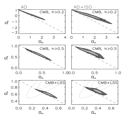
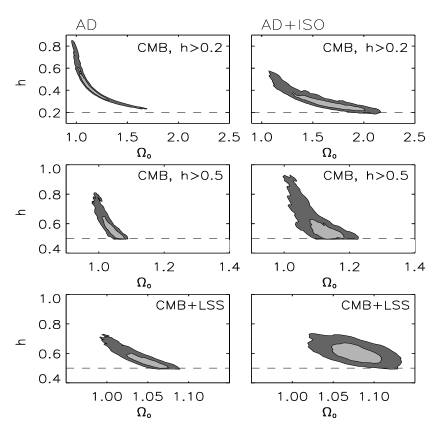
We first explored the determination of the spatial curvature allowing only the adiabatic models, characterised by seven parameters (eight with LSS), and including various combinations of data sets. With only the CMB data and the weak prior $0.2<h<1$, the curvature is poorly constrained as shown in Table 1. The CMB provides a good measure of the angular diameter distance $d_{AD}=(z_{rec}+1)d^{*}_{rec}/\theta^{*}$, but a degeneracy exists between the curvature and the conformal distance to last-scattering $d_{LS}$geom , as illustrated in the top-left panels of Figs. 2 and 3. $d_{LS}$ increases with decreasing $h$ or $\Omega_{\Lambda}$ and with increasing $\Omega_{m}.$ The constraint on the geometry is considerably tightened when $h>0.5$ is imposed. The degeneracy is also broken by the LSS data. The shape of the power spectrum constrains $\Omega_{m}h,$ ruling out the closed models with high $\Omega_{m}$ allowed by the CMB data, which instead constrains $\Omega_{m}h^{2}$. Similarly supernova luminosity-redshift measurements exclude models with high $\Omega_{m}$ and low $\Omega_{\Lambda}$, as shown in Fig. 2. By including CMB, LSS, SNIa and HST data combined, the geometry is strongly constrained to $\Omega_{0}=1.01\pm^{0.02}_{0.01}$, in agreement with wmap_param ; sloan_param .

Figure 4: CMB temperature (top) and galaxy power spectra (bottom) for a curved cosmological model dominated by isocurvature with $f_{iso}=90\%$, $\Omega_{0}=1.9$. It fits current CMB data well (TT and TE), but does not fit LSS data and is inconsistent with BBN and HST observations ($\omega_{b}=0.08$, $h=0.3$).

Dataset	$h$	$\Omega_{0}$	$\langle f_{iso}\rangle$
cmb	$>0.2$	$1.6\pm 0.3$	$0.6$
cmb	$>0.5$	$1.10\pm 0.05$	$0.6$
cmb + lss	$>0.2$	$1.07\pm 0.03$	$0.5$
cmb + lss	$>0.5$	$1.07\pm 0.03$	$0.5$
cmb + lss +snia	$0.72\pm 0.08$	$1.06\pm 0.02$	$0.54$
cmb + lss +bbn	$>0.5$	$1.06\pm 0.03$	$0.31$

Table 2: Median and $68\%$ confidence intervals for $\Omega_{0}$ and median isocurvature fraction $f_{iso}$ for models with mixed initial conditions.

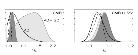
We now consider how the measurements are affected when the full range of correlated isocurvature and adiabatic initial conditions are admitted. Initially the spectral indices of the modes are fixed as a single parameter, giving rise to a family of models described by sixteen parameters (seventeen with LSS). Figs. 2, 3 and 5 and Table 2 demonstrate that the determination of the geometry of the Universe is significantly degraded by the inclusion of these additional degrees of freedom. As in the adiabatic cases, where $\Omega_{0}=1.2\pm^{0.2}_{0.1}$ results from the CMB data alone, the data favor a closed Universe with $\Omega_{0}=1.6\pm 0.3$ when isocurvature is allowed, with the priors $h>0.2$ and $\Omega_{d}<3$ constraints cutting off larger curvatures. The extremely closed models, such as the one in Fig 4, are dominated by up to 90% isocurvature (at 2$\sigma$), and exhibit low $h$, high $\Omega_{m}$ and low $\Omega_{\Lambda}$, extending the degenerate direction observed for the adiabatic models. Many models dominated by the NIV mode require a high baryon content ($\omega_{b}\approx 0.06$), so the acoustic peak positions are shifted to smaller scales by lowering the sound speed at recombination. This effect contributes to the exclusion of isocurvature-dominated extreme open models. Closed models dominated by the NID or CI modes do not fit the CMB data, particularly at large scales.

Additional data constraining $d_{LS}$ improve the curvature constraints. The prior $h>0.5$ alone suffices to exclude highly closed models. Alternatively, the LSS data constrains the allowed range to $\Omega_{0}=1.07\pm 0.04$ in two ways. Firstly, its shape constrains $\Omega_{m}h$ and rules out high $\Omega_{m}$ models, since in most models the matter power spectrum is dominated by the adiabatic mode. Secondly, the LSS data rules out models dominated by NIV, which predict significant baryon oscillations. The supernova and HST data further constrain $d_{LS}$. The combination of all datasets gives $\Omega_{0}=1.06\pm 0.02$, with $\langle f_{iso}\rangle=0.54$. The distribution for $f_{iso},$ however, is very broad and does not appear to disfavor the adiabatic models. Within this class of models the data prefer higher baryonic densities ($\omega_{b}=0.04\pm 0.02$ for CMB+LSS data) than consistent with nucleosynthesis measurements. We find that adding the Gaussian prior $\omega_{b}=0.022\pm 0.002$ from recent BBN measurements bbn to the CMB+LSS analysis with the prior $h>0.5$ reduces the isocurvature contribution by just under a half and yields $\Omega_{0}=1.06\pm 0.03.$

Figure 5: Marginalized posterior distributions for $\Omega_{0}$ for adiabatic models (ad,unshaded) and mixed initial conditions with common spectral indices (ad+iso, shaded). The dark shaded and dashed curves show results for $h>0.5$, otherwise $h>0.2$.

We also repeated the analysis for an enlarged space of models where each of the isocurvature modes is given an independent tilt within the range $0<n_{i}<2$. The resulting twenty-dimensional model constrained by CMB+LSS with the $h>0.5$ prior gives $\Omega_{0}=1.08\pm 0.03$ and the following constraints on the spectral indices: $n_{\mbox{\tiny{AD}}}=1.1\pm 0.2$, $n_{\mbox{\tiny{CI}}}=1.1\pm 0.5$, $n_{\mbox{\tiny{NID}}}=1.4\pm 0.3$, $n_{\mbox{\tiny{NIV}}}=1.1\pm 0.3$, with isocurvature fraction $\langle f_{iso}\rangle=0.5$. The region of high probability density, however, includes models with virtually no isocurvature. We do not find that the models with isocurvature modes offer a better fit than the adiabatic models, beyond what may generically be expected as a result of enlarging the number of degrees of freedom of the theoretical model. This result is analogous to the flat case considered in bdfms .
In this letter, we have substantially strengthened the evidence for an almost flat Universe, with the data suggesting a slight preference for a mildly closed Universe. In considering a very general class of initial conditions, we have removed the assumption of adiabaticity and hence on specific models of the early universe such as inflation. In principle this could have completely removed the ability to constrain the geometry of the Universe with current data sets, as was shown in bmt_2002 . Indeed we find with this wider range of parameters a behavior similar to what has already been noted for purely adiabatic initial conditions: that the CMB alone does not suffice to constrain the geometry of the Universe. Once one includes additional information (constraining $h$ or $\Omega_{m}h$), it is possible to pin down the geometry with appreciable precision. Consequently, for very general initial conditions where perturbations are imprinted at early times and subsequently evolved through gravitational collapse, we conclude that the Universe is very nearly flat.
Acknowledgements: We thank O. Lahav and R. Trotta for discussions. J.D. and C.S are supported by PPARC.

References

- (1) A. G. Doroskevich, Y. Zeldovich & R. Sunyaev, Sov. Astron. 22, 523 (1978).
- (2) .
- (3) A. D. Miller et al., Astrophys. J. 524., 1 (1999); P. D. Mauskopf et al., Astrophys. J. 536, 59 (2000); S. Hanany et al., Astrophys. J. 545, 5 (2000).
- (4) G. Hinshaw et al., Astrophys. J. 148, 135 (2003); A. Kogut et al., Astrophys. J. 148, 161 (2003).
- (5) M. Bucher, K. Moodley and N. Turok, Phys. Rev. D 66, 023528 (2002).
- (6) W. L. Freedman et al., Astrophys. J. 553, 47 (2001).
- (7) M. Tegmark et al., Phys. Rev. D 69, 103501 (2004).
- (8) D. N. Spergel et al., Astrophys. J. 148, 213 (2003).
- (9) W. J. Percival et al., Mon, Not. R. Astron. Soc, 327, 1297 (2001).
- (10) M. Tegmark et al., Astrophys. J. 606, 702-740 (2004).
- (11) J. L. Tonry et al., Astrophys. J. 594, 1 (2003).
- (12) J. R Bond and G. Efstathiou, Mon. Not. R. Astron. Soc. 22, 33 (1987); P. J. E. Peebles, Nature 327, 210 (1987); A. Rebhan and D. Schwarz, Phys. Rev. D 50, 2541 (1994); A. Challinor and A. Lasenby, Astrophys. J. 513, 1 (1999), 531 (1999); M. Bucher, K. Moodley and N. Turok, Phys. Rev. D. 62, 083508 (2000).
- (13) H. V. Peiris et al., Astrophys. J. Suppl. Ser. 148, 213 (2003); P. Crotty et al., Phys. Rev. Lett. 91, 171301 (2003); C. Gordon and K. A. Malik, astro-ph/0311102 (2003); H. Kurki-Suonio, V. Muhonen and J. Valiviita, Phys. Rev. D 71, 063005 (2005).
- (14) M. Bucher et al., Phys. Rev. Lett. 93, 081301 (2004); K. Moodley et al., Phys. Rev. D 70, 103520 (2004).
- (15) http://camb.info; A. Lewis, A. Challinor and A. Lasenby, Astrophys. J. 538, 473 (2000).
- (16) L. Verde et al., Astrophys. J. Suppl. Ser. 148, 195 (2003).
- (17) X. Wang et al., Phys. Rev. D 68, 123001 (2003).
- (18) C. L. Kuo, et al., Astrophys. J. 600, 32 (2004); J. Ruhl et al., Astrophys. J, 599, 786 (2003); T. J Pearson et al., Astrophys. J. 591, 556 (2003); P. F. Scott et al., Mon. Not. R. Astron. Soc. 341 1076 (2003).
- (19) R. E. Smith et al., Mon, Not. R. Astron. Soc, 341, 1311 (2003).
- (20) J. Dunkley et al., Mon, Not. R. Astron. Soc, 356, 925 (2005).
- (21) M. Kaplinghat, L. Knox and C. Skordis, Astrophys. J. 578, 665 (2002).
- (22) J. R. Bond, G. Efstathiou & M Tegmark, Mon, Not. R. Astron. Soc 291, 33 (1997).
- (23) B. D. Fields & S. Sarkar, Phys. Rev. D 66 010001 (2002).