A New Technique for Probing Convection in Pulsating White Dwarf Stars

Abstract

In this paper we demonstrate how pulsating white dwarfs can be used as an astrophysical laboratory for empirically constraining convection in these stars. We do this using a technique for fitting observed non-sinusoidal light curves, which allows us to recover the thermal response timescale of the convection zone (its “depth”) as well as how this timescale changes as a function of effective temperature. We also obtain constraints on mode identifications for the pulsation modes, allowing us to use asteroseismology to study the interior structure of these stars. Aspects of this approach may have relevance for other classes of pulsators, including the Cepheids and RR Lyrae stars.

1. Astrophysical Context

The physics of convection represents one of the largest sources of uncertainty in modeling stars. In main sequence objects, convection is believed to occur in the cores of stars more massive than the Sun (e.g., Woo & Demarque, 2001) as well as in the envelopes of stars having masses less than about $2.0\,M_{\odot}$. Red Giant stars should have fully convective envelopes (e.g., Salaris, Cassisi, & Weiss, 2002), making convection common throughout the H-R diagram. Along the white dwarf cooling track we expect white dwarfs with helium spectra (DBs) and temperatures less than $\sim\,$35,000 K to have surface convection zones, while those with hydrogen spectra (DAs) and temperatures less than $\sim\,15,000$ K should also have convective surface layers.

The fact that there are major uncertainties in our ability to model the physics of convection has significant astrophysical consequences. For instance, whether or not convective overshoot occurs in the cores of massive stars affects the amount of material which is available for nuclear burning, leading to an uncertainty of $\sim\,20\,$% in stellar ages (Di Mauro et al., 2003; Bitzaraki et al., 2001). For pulsating white dwarfs, uncertainty regarding convection in their atmospheres is the largest single source of error in their derived effective temperatures (e.g., Bergeron et al., 1995). This is significant since we use what we learn about the interior structure of the pulsators to calibrate white dwarf cooling sequences, which in turn can be used to determine the ages of individual white dwarfs (Ruiz & Bergeron, 2001) or the age of the Galactic disc (Wood & Oswalt, 1998; Wood, 1992; Winget et al., 1987).

The very low-amplitude oscillations which have been observed in the Sun and recently in other Solar-like stars (e.g., Bedding & Kjeldsen, 2003) have traditionally been explained through stochastic driving due to the outer convection zones found in these stars (e.g., Kumar, Franklin, & Goldreich, 1988; Houdek et al., 1999). However, one of the first results from the Canadian space mission MOST (Microvariability and Oscillations of STars) has been that the oscillations expected in the star Procyon are not present, at least not at detectable levels (Matthews et al., 2004), implying that our understanding of convection in stars even slightly more massive than the Sun may still be incomplete.

In the sections which follow we describe a new technique for fitting observed non-sinusoidal light curves in white dwarfs. With this technique we can recover the thermal response timescale of the convection zone (or its depth) and how this timescale changes as a function of effective temperature. We also obtain mode identifications for the pulsation modes, which helps us to use asteroseismology to study the interior structure of these stars.

Our approach for deriving information on the depth of the convection zone and its temperature sensitivity is based on the seminal numerical work of Brickhill (1992) and on the complementary analytical treatment of Goldreich & Wu (1999) and Wu (2001). Essentially, we take a hybrid of these two approaches, and it is this model which we describe below.

2. The Model

2.1. Assumptions

The fundamental assumptions of our hybrid model are that:

1. The flux perturbations beneath the convection zone are sinusoidal in time and have the angular dependence of a spherical harmonic.

2. The convection zone is so thin that we may locally ignore the angular variation of the nonradial pulsations, i.e., we treat the pulsations locally as if they were radial.

3. The convective turnover timescale is so short compared to the pulsation periods that the convection zone can be taken to respond “instantaneously”.

4. Due to the extreme sensitivity of the convection zone to changes in temperature, we consider only flux and temperature variations, i.e., the large-scale fluid motions associated with the pulsations are ignored.

The third assumption is given weight by appeal to standard convection models of these stars, which indicate that the time taken for a convective fluid element to circulate from top to bottom of the convection zone should be less than a second. Since the pulsation periods of these stars are much longer than this, i.e., hundreds of seconds, this appears to be a safe assumption. While plausibility arguments for the other assumptions may similarly be made, it is perhaps better to see how well they allow us to model the observed light curves before deciding on their viability (“the proof is in the pudding”).

2.2. Energetics

We assume energy conservation in that the flux emitted at the photosphere, $F_{\rm phot}$, is equal to the flux incident at the base of the convection zone, $F_{\rm base}$, minus the energy per unit time which is absorbed by the convection zone, $d\tilde{Q}/dt$, i.e.,

$$F_{\rm phot}=F_{\rm base}-\frac{d\tilde{Q}}{dt}.$$ (1)

Physically, this can be thought of as the convection zone having a specific heat; it must absorb some amount of energy for its photospheric temperature to be raised by a given amount.

Due to the assumption that the convection zone is instantaneously in quasi-static equilibrium, we can compute the term $d\tilde{Q}/dt$ purely in terms of static envelope models having different values of $T_{\rm eff}$ (see Wu, 2001, eq. 4). This energy absorption rate depends only on the photospheric flux (or $T_{\rm eff}$), leading to the following equation:

$$F_{\rm phot}=F_{\rm base}+\tau_{C}\frac{dF_{\rm phot}}{dt},$$ (2)

where the new timescale $\tau_{C}\equiv\tau_{C}\mbox{\scriptsize$(F_{\rm phot})$}$ describes the changing heat capacity of the convection zone as a function of the local photospheric flux. Thus, we have reduced the problem to a first-order, ordinary differential equation in time. Since the perturbations at the base of the convection zone are assumed to be linear, $F_{\rm base}$ is taken to have the usual time and angular dependence of a nonradial oscillation mode, i.e.,

$$F_{\rm base}={\rm Re}\,[\,A\,e^{i(\omega t+\delta)}Y_{\ell m}(\theta,\phi)],$$ (3)

so equation 2 must be solved on a grid of points across the visible surface of the star having different values of $\theta$ and $\phi$, and the resulting fluxes need to be added together to calculate the observed light curve (note: $A$ and $\delta$ in equation 3 are the amplitude and phase associated with the pulsation mode, respectively). Fortunately, because of the simplifications we have introduced, this problem is still computationally tractable.

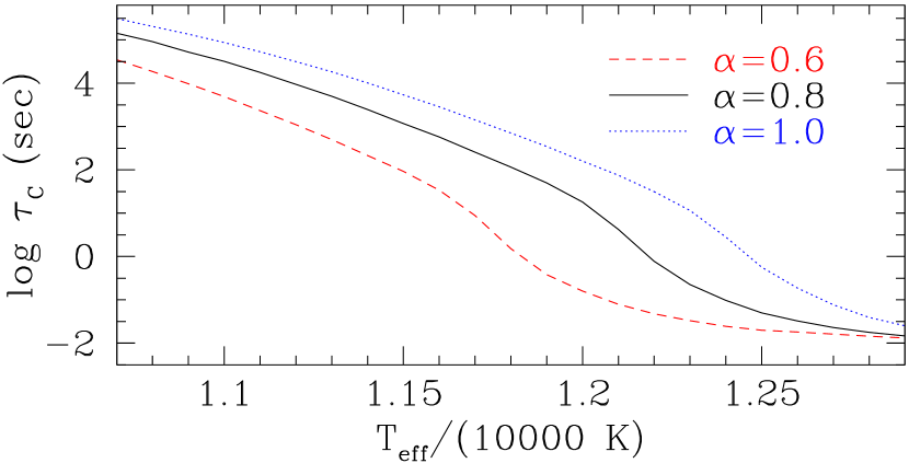
In Figure 1, we show a theoretical calculation of how this timescale $\tau_{C}$ is expected to vary as a function of $T_{\rm eff}$. For a given value of $\alpha$ (the mixing length to pressure scale height ratio), we see that $\tau_{C}$ changes by approximately a factor of 1000 as the temperature goes from 12000 K (the observed onset of pulsations in DAVs) to 11000 K (the observed disappearance of pulsations in DAVs). If we parameterize this as a power law in $T_{\rm eff}$, i.e.,

$$\tau_{C}\approx\tau_{0}T_{\rm eff}^{-N},$$ (4)

we find that $N\approx$ 90–95 and $\tau_{0}$ is a function of $\alpha$, demonstrating a very strong temperature dependence (the curves in Fig. 1 were computed using the standard mixing length theory of Böhm & Cassinelli, 1971). We note that although the value of $\tau_{0}$ is affected by the version of mixing length theory employed and the choice of $\alpha$, e.g., Böhm-Vitense (1958) versus Böhm & Cassinelli (1971), the value of $N$ inferred from these standard models is relatively constant, having values in the range 90–95 in the DAV instability strip; for the DBVs, we find $N\approx$ 20–23. The simplified convection model used by Wu (1997), while still quite temperature sensitive, has a value of $N\approx 55$ for DAV models. As we will see, the observations can be used to constrain the value of $N$. For comparison with previous work by Wu, we note that in terms of her variables that $N\approx 2\beta+\gamma$.

Figure 1.— Theoretical calculations of the thermal response timescale of the convection zone, $\tau_{C}$, as a function of $T_{\rm eff}$. The local mixing-length theory of Böhm & Cassinelli (1971) has been used (ML2), for the given values of $\alpha$.

Since a typical pulsator may have excursions in temperature of several hundreds of degrees, we expect $\tau_{C}$ to vary greatly during the pulsations, leading to nonlinear light curves. Indeed, nonlinearities beyond second order can become important, making it possible to constrain not only $\tau_{0}$ but also the other parameters of the fit, such as $N$, the inclination angle $\theta_{\rm i}$, as well as the $\ell$ and $m$ values of the pulsation mode.

Since the fluxes in equations (1)–(3) refer to the total energy being gained and lost by the convection zone, they represent bolometric fluxes. By using sequences of static, numerically computed envelopes to connect conditions at the base of the convection zone with those at the photosphere, we implicitly have taken into account the $T^{4}$ nonlinearities associated with variations in the photospheric temperature. However, since the observations that are typically made are in a finite wavelength range which is well-separated from the peak wavelength flux, we must apply a correction factor for the computed fluxes when comparing with the observations.

For data taken with phototubes, we assume that the observations are taken in a narrow bandpass centered on 4300 Å, and for CCD data taken with the ARGOS photometer we assume a central wavelength of 5000 Å (Nather & Mukadam, 2004). The simplified model for the correction factor which we employ here assumes a blackbody distribution for the radiative flux, which we then linearize about the effective temperature; we apply this correction individually to each element of surface area at each time step. In practice, this bolometric correction leads to a reduction in the observed pulsation amplitudes of $\sim 1.5$ for the DAVs and $\sim 2.4$ for the DBVs. Finally, we note that we have used the same simplified limb-darkening law as Wu for both the DAVs and DBVs, namely the Eddington limb-darkening law:

$$h(\mu)=1+\frac{3}{2}\,\mu,$$ (5)

where $\mu$ is the cosine of the angle between a surface normal vector and the line-of-sight.

3. Lightcurve fitting

In this section we examine how the hybrid model represented by equations (2)–(4) compares with the model of Wu (1997, 2001), both for synthetic data and for actual observations of stars.

Figure 2.— Test fits of synthetic light curves having no angular dependence. In the lower panel of (a) we show the synthetic data (crosses) and our fit (solid curve), and in the upper panel we show the thermal response timescale used to generate the synthetic light curve (solid curve) compared with that which we derive from our fit (dashed curve). The vertical dotted lines indicate the maximum and minimum temperature excursions which the photosphere undergoes during a pulsation cycle. (b) The same as (a) but using Wu’s second-order expression for the light curve fits.

Wu’s model uses the harmonics and combination frequencies that arise from the second-order solution of equations (2)–(4). For a single mode with harmonics, Wu’s model constrains $\tau_{0}$, but the quantities $N$, $\theta_{\rm i}$, and the amplitude are degenerate with respect to each other. This is a result of using only the lowest-order nonlinear terms.

Our approach is to numerically solve equations (2)–(4), so we implicitly include the contributions of all the nonlinear terms, including those of higher order. Thus, by using more of the information present in the light curves we hope to remove the degeneracies in the fits.

The technique developed by Wu was designed to be used for the amplitudes and phases as derived from a Fourier transform of the data. For consistency, we prefer to make comparisons directly with the light curves, so we use her formulae to generate trial light curves which are then fitted to the data.

3.1. Tests omitting angular structure

In this section we omit the angular structure and study fits to the emergent flux from a fixed surface element using synthetic data; this is formally equivalent to examining pulsations having $\ell=0=m$. In addition to the convective parameters $\tau_{0}$ and $N$, we fit the amplitude $A$ and phase $\delta$ in equation 3; the frequency is assumed known from the observations. Since there is no ambiguity associated with the choice of an inclination angle, we expect that the method of Wu, along with our method, will lead to non-degenerate best fit solutions.

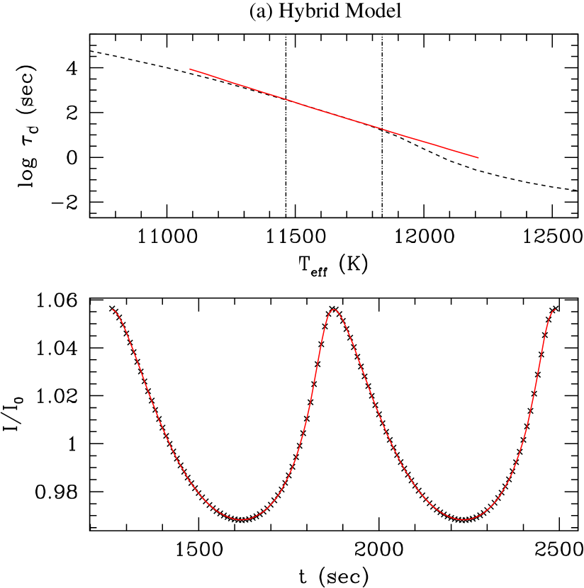
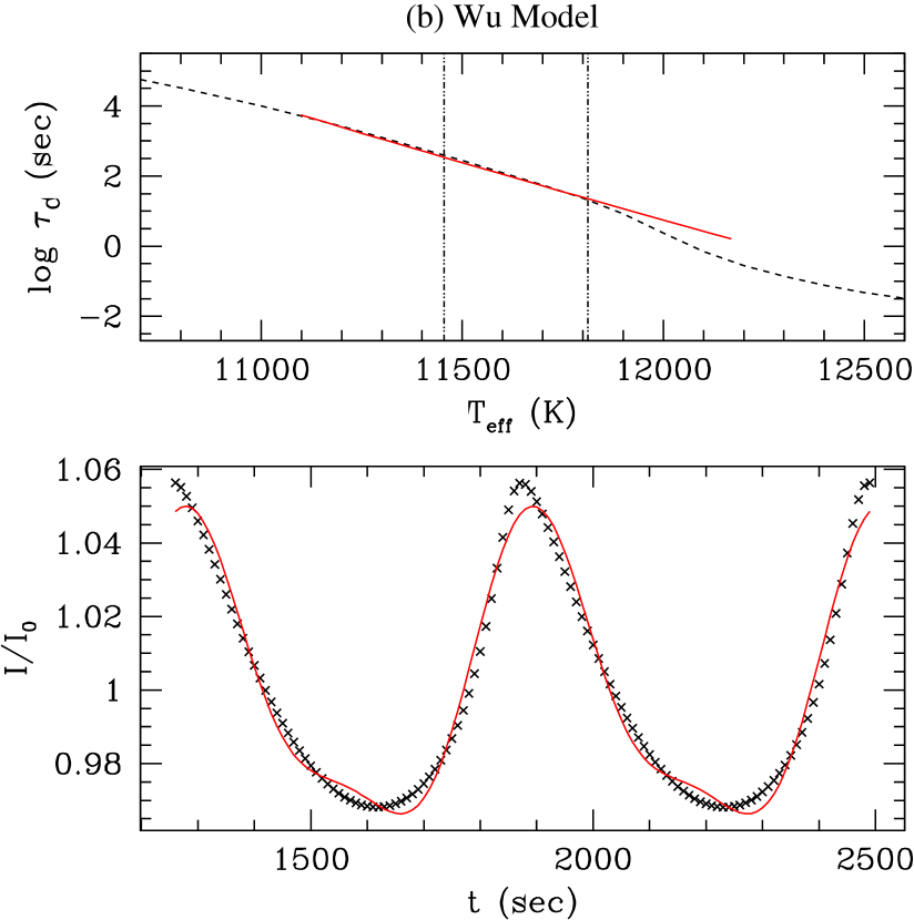
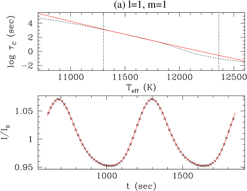
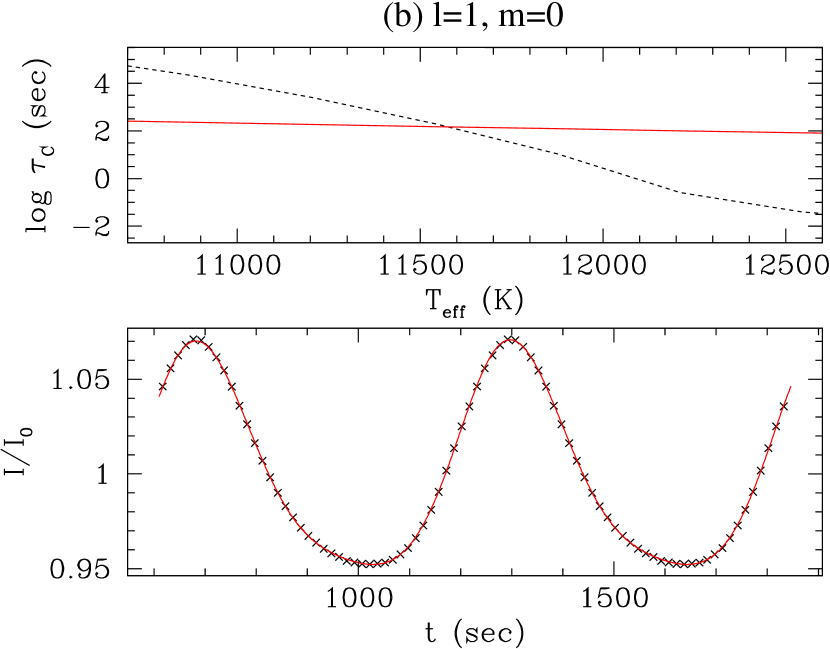
In Fig. 2 we show fits to synthetic (test) light curves using (a) our hybrid models and (b) Wu’s second-order expression. To compute the synthetic light curve in this test we have assumed that the thermal response timescale of the convection zone, $\tau_{C}$, is given by local MLT models such as the curves shown in Fig. 1. Thus, the only difference between the input model and our fits is that our fits assume the simplified form for $\tau_{C}$ given by equation 4. The adequacy of this assumption can be seen in Fig. 2a which shows that not only is the light curve reproduced well (lower panel) but also that the match between the input $\tau_{C}$ and that derived from the fit is quite good (upper panel). In Fig. 2b, we show the same comparisons using Wu’s second-order expressions for the flux perturbations. In the lower panel we see that this provides a reasonable qualitative fit to the synthetic light curve, although the marked discrepancies between light curve and the fit arise from neglecting the higher order terms. In the upper panel we see that the slope of the derived $\tau_{C}$ is fairly close to that of the input model.

Table 1Summary of test fits without noise

model	$\theta_{\rm i}$(deg)	$\tau_{0}$ (sec)	$N$	Amp	$\ell$	$m$	MSD
input model	—	123.8	93.1	0.100	0	0	—
hybrid model	—	122.5	94.9	0.100	0	0	0.014
Wu model	—	109.0	89.7	0.088	0	0	8.272
input model	56.0	123.8	93.1	0.070	1	0	—
hybrid model	54.5	122.3	99.5	0.067	1	0	0.001
hybrid model	0.0	118.4	71.4	0.067	2	0	0.021
Wu model	—	111.2	—	—	—	—	1.343
hybrid model	83.1	162.0	359.4	0.094	1	1	0.369

The parameters associated with these fits are presented in the upper part of Table 1. The goodness of fit is measured by the mean-squared deviation (MSD), defined by

$$\mbox{MSD}\equiv\frac{1}{N}\sum_{i=1}^{N}\,[I_{\rm obs}(i)-I_{\rm calc}(i)]^{2},$$ (6)

where $I_{\rm obs}$ and $I_{\rm calc}$ are the observed and theoretically calculated light curves which have been normalized to an average value of 1, respectively, and $N$ is the number of data points. We see that the fit using the hybrid model is able to recover the parameters of the input model quite well. Although the Wu model fit has much higher residuals, it too reproduces the parameters of the input model fairly well.

Figure 3.— Upper panel: The best fit residuals as a function of $\theta_{\rm i}$. Lower panel: Contours of constant fit residuals showing the relationship between the intrinsic amplitude of the mode and $\theta_{\rm i}$. The minimum on the right corresponds to the $\ell=1$, $m=0$ solution, and the minimum on the left corresponds to the $\ell=2$, $m=0$ solution. The cross indicates the parameters of the input model.

3.2. Tests including angular structure

We now repeat the tests of the previous section, this time incorporating the expected angular structure of the pulsation modes into the calculation. In addition to the quantum numbers $\ell$ and $m$ which now must be taken into account, the light curve shape also becomes a function of the inclination angle, $\theta_{\rm i}$. For the fits, we have initially varied $\theta_{\rm i}$ in 1^∘ increments, and in the neighborhood of the minimum we have decreased the increments to 0.1^∘.

In addition, we must discretize the surface of the stellar model and sum over all elements to calculate the light curve. In order to minimize the number of computations for a given accuracy, we discretize the surface of the model so that the surface area of each element projected along the line-of-sight is the same. Thus, elements near the edge of the disc contribute with the same weight (except for limb-darkening). Each of the elements is wedge-shaped and they are arranged radially on annuli centered on the the visible disc of the model. The input models were calculated using 1024 surface elements arranged on 16 annuli, and the subsequent fits to these models and fits elsewhere in this paper have used 256 elements arranged on 8 annuli.

In Wu’s second-order theory, a degeneracy exists among the parameters such that it is not possible to disentangle $\theta_{\rm i}$ from the intrinsic mode amplitude or from the thermal timescale parameter $N$, i.e., equally good fits are possible for any value of $\theta_{\rm i}$. Our hope is that the inclusion of the higher-order nonlinear effects in our hybrid model will lift this degeneracy and allow unique fits to be made.

In the lower part of Table 1 we show the results of different fits to a sample light curve having $\ell=1$, $m=0$, and $\theta_{\rm i}$ $=56.0^{\circ}$ (these values are similar to those derived in Section 3.4.2 for PG1351+049). Based on the residuals, the hybrid model with $\ell=1$, $m=1$ can be ruled out, as can be the Wu model, although it again provides a reasonable estimate of $\tau_{0}$. The remaining hybrid models both have very low residuals, making a choice between the two difficult.

Figure 4.— The same plot as Fig. 2 but for the best fit solution of Figure 3.

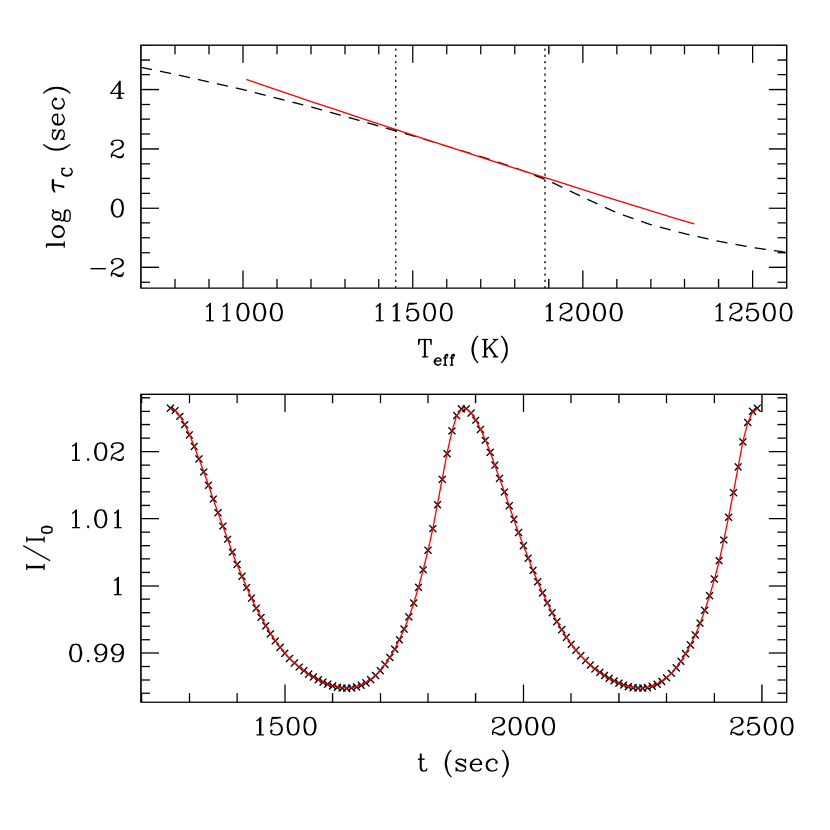
In Figure 3 we examine the uniqueness of the mode identifications as well as possible degeneracies in the fit parameters. In the upper panel the residuals of the two best fits are plotted as a function of $\theta_{\rm i}$, and in the lower panel contours of constant residuals of these fits are shown as a function of $\theta_{\rm i}$ and mode amplitude. We see that while there is a partial degeneracy between $\theta_{\rm i}$ and the amplitude $A$, the presence of the higher-order nonlinearities does indeed lift this degeneracy and allow a unique solution to be obtained. This best-fit solution is shown in Figure 4.

Although no noise has been added to the synthetic light curve, the derived value of $\theta_{\rm i}$, 54.5^∘, does differ slightly from the input value of 56.0^∘. This is because for finite amplitude pulsations the parameterization in equation (4) for $\tau_{C}$ does not exactly reproduce the variations in $\tau_{C}$ of the input model.

From the above fits, we see that a mode with $\ell=1$, $m=0$, and $\mbox{$\theta_{\rm i}$}=56^{\circ}$ can be mimicked by a mode with $\ell=2$, $m=0$, and $\theta_{\rm i}$$=0^{\circ}$; indeed, even the amplitudes which are derived in these two cases are nearly identical. While more work is needed to address the cause of this similarity, we find from exploratory calculations that the degeneracy between these mode pairs exists only when $\mbox{$\theta_{\rm i}$}>45^{\circ}$ for the $\ell=1$ mode.

Table 2Summary of test fits including noise

model	$\theta_{\rm i}$(deg)	$\tau_{0}$ (sec)	$N$	Amp	$\ell$	$m$	MSD
input model	56.0	123.8	93.1	0.070	1	0	—
hybrid model	51.5 $\pm$ 5.2	127.1 $\pm$   9.0	-108.6 $\pm$ 16.9	0.066 $\pm$ 0.009	1	0	0.459 $\pm$ 0.056
hybrid model	0.3 $\pm$ 0.5	118.5 $\pm$   6.5	-69.8 $\pm$   2.4	0.067 $\pm$ 0.002	2	0	0.437 $\pm$ 0.081
hybrid model	84.0 $\pm$ 1.3	212.6 $\pm$ 51.4	-355.1 $\pm$ 10.1	0.111 $\pm$ 0.019	1	1	1.711 $\pm$ 0.168
hybrid model	85.1 $\pm$ 1.4	104.2 $\pm$ 11.5	-3.0 $\pm$   1.8	0.620 $\pm$ 0.148	2	1	1.779 $\pm$ 0.153
hybrid model	0–90	100–110	0	0.16–0.40	2	2	10–11

Figure 5.— The same plot as Fig. 4 but for Gaussian noise added to the synthetic light curve.

3.3. Tests including noise

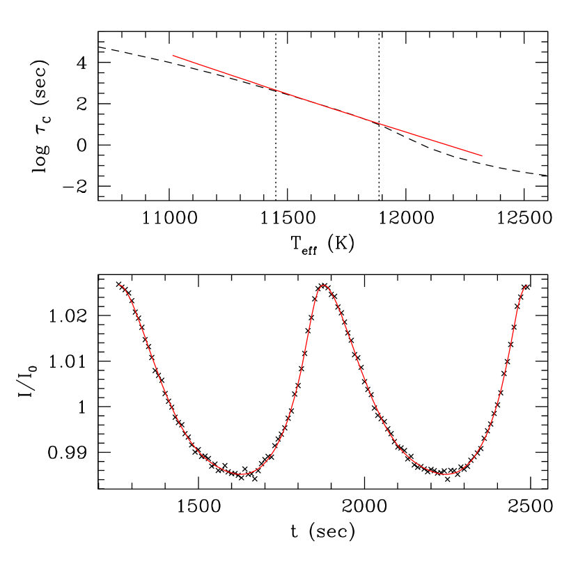
In this section we examine the effect of Gaussian noise on our light curve fits. In Figure 5 we show an example of such a fit, where the level of the noise has been chosen to be somewhat higher than the data which will be analyzed in section 3.4. In Table 2 we show the results of many different fits to the given input model for solutions having different $\ell$ and $m$ values. The parameter values and their error bars listed in the table were obtained by computing the average and standard deviation of fit values for 10 different realizations of the noise. In the case of the $\ell=2$, $m=2$ fit, the fits are so poor that there is no single “best fit”; for this case, we have simply indicated the allowed ranges for the parameters.

Unsurprisingly, the two fits having the lowest residuals are the same ones as in the noise free case, and the difference in their residuals is not statistically significant. Thus, choosing between them on the basis of their residuals alone is not possible, and we are indeed faced with the problem of non-uniqueness. As in the noise free case, however, these fits still provide a good estimate of $\tau_{0}$ and the amplitude, and the $\ell=2$ solution gives a decent estimate of $N$.

Examining the results of this and the previous sections, we see that the hybrid model is able to accurately derive many of the parameters of the input model, both for the case with and without noise. Indeed, the model of Wu can also provide reasonably good estimates of $\tau_{0}$, although not of the other parameters due to the degeneracy between $\theta_{\rm i}$, $N$, and the amplitude. While fits to actual data will of course be more difficult, these results give us hope that we will be able to derive meaningful constraints on the parameters through such a fitting procedure.

3.4. Fits to observations

Since we are using a new technique, we wish to start with the best possible candidates, i.e., those for which the application of the method is the most straightforward. For the present application, we therefore restrict ourselves to stars which (1) are mono-periodic, having one oscillation mode which dominates their light curves, (2) have large-amplitudes, so that their light curves contain clear nonlinearities, and (3) have high signal-to-noise data, so that the errors are as small as possible. In future work we will examine the degree to which these criteria can be relaxed, while the focus of our present work is to demonstrate that the method does indeed work for the cases examined below.

While by no means an exhaustive list, two stars fill these requirements admirably: the DBV PG1351+049 and the DAV G29-38. Both stars have light curves which are nearly mono-periodic (at least during the time the observations were made), have significant nonlinearities, and high quality data are available for both. In the following two sections we describe the fits to these data.

Figure 6.— Lower panels: fits (solid curve) to the observed pulse shape (crosses) of the DAV star G29-38 for observations taken in 1988. Upper panels: the empirically derived $\tau_{C}$ as a function of $T_{\rm eff}$ (solid curve) versus that calculated assuming a given mixing-length theory (dashed curve). The fit on the left assumes $\ell=1$, $m=1$, while the fit on the right assumes $\ell=1$ and $m=0$.

Table 3Derived parameters for G29-38

$\theta_{\rm i}$(deg)	$\tau_{0}$ (sec)	$N$	Amp	$\ell$	$m$	MSD
65.5 $\pm$ 3.4	187.4 $\pm$ 20.3	95.0 $\pm$ 7.7	0.259 $\pm$ 0.011	1	1	0.160 $\pm$ 0.045
73.9  $\pm$ 0.7	150.1 $\pm$   6.5	7.1 $\pm$ 0.6	0.417 $\pm$ 0.025	1	0	0.178 $\pm$ 0.035
31.9  $\pm$ 1.3	151.2 $\pm$   7.4	5.8 $\pm$ 0.6	0.363 $\pm$ 0.022	2	0	0.171 $\pm$ 0.037
82.0  $\pm$ 0.8	139.4 $\pm$   3.9	1.6 $\pm$ 0.4	1.190 $\pm$ 0.098	2	1	0.382 $\pm$ 0.028
$\sim$80.0	$\sim$110	0.0	$\sim$0.27	2	2	$\sim$41.0

3.4.1 The DAV G29-38

The light curve of the DAV G29-38 was obtained by S. Kleinman in 1988 (Winget et al., 1990; Kleinman, 1995). Due to the very long time baseline of the observations, the resulting folded light curve/pulse shape has a very high signal-to-noise. We show this light curve, folded at a period of 615.15 s, along with two different fits to it, in the lower panels of Figure 6: the crosses are the folded light curve and the solid curve are the fits to it. The fit on the left is for an $\ell=1$, $m=1$ pulsation mode, while that on the right is for an $\ell=1$, $m=0$ mode.

From Table 3 we see that these two fits, along with the $\ell=2$, $m=0$ fit, have residuals which are not statistically different from one another. However, they imply vastly different temperature sensitivities (i.e., $N$) for the thermal response timescale of the convection zone. In particular, if white dwarf convection zones were as weak a function of $T_{\rm eff}$ as implied by either the $\ell=1$, $m=0$ or the $\ell=2$, $m=0$ solution ($N\sim$ 5–7), there would hardly be any change in depth of their convection zones as they cross the ZZ Ceti instability strip. This runs counter to all theoretical predictions of convection, whether based on MLT or on numerical hydrodynamic simulations (Freytag, 1995). We conclude that the physically meaningful solution is the $\ell=1$, $m=1$ solution. This yields a value of $N\approx 95$, which is exactly in the range predicted by standard models of convection. In addition, we note the identification $\ell=1$ is consistent with that found by Clemens et al. (2000) from an examination of the wavelength dependence of the pulsation amplitude.

3.4.2 The DBV PG1351+049

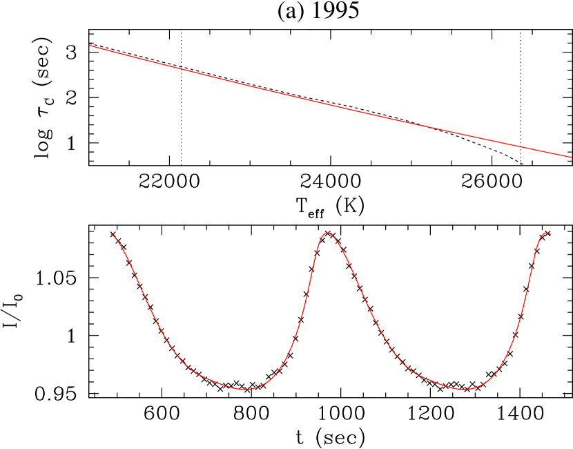
In 1995 the DBV star PG1351+049 was observed as part of a Whole Earth Telescope (WET; Nather et al., 1990) campaign (e.g., Winget et al., 1991, 1994). In 2004, we re-observed this star using the Argos CCD photometer on the McDonald 2.1m telescope. This second set of high quality observations is important because it allows us to cross check this technique. If we really are learning about the fundamental parameters of the star then we would not expect those parameters to have changed, i.e., the average depth of the convection zone, $\tau_{0}$, and the inclination angle, $\theta_{\rm i}$, should be the same, although other quantities such as the amplitude of the mode might very well be different.

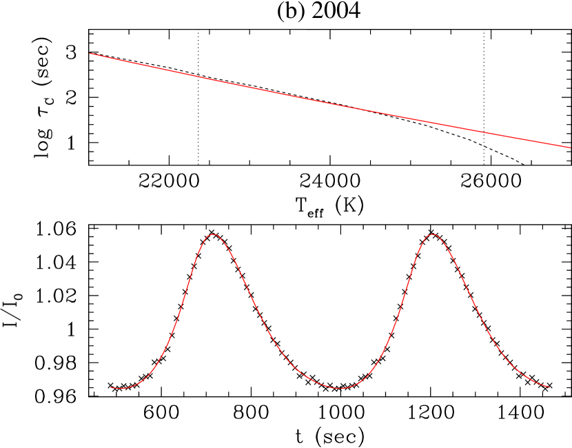
As we saw in the previous section, a degeneracy in the parameters can occur so that two sets of parameters produce roughly equivalent fits. This is also the case for this star; we find both an $\ell=1$, $m=0$ fit and an $\ell=2$, $m=0$ fit which reproduce the data well.

In Figure 7, we show the results of the $\ell=1$ fits. The data have been folded at the period of the mode, 489.335 s, to improve signal-to-noise and to simplify the fitting. We note that the fit is very good and reproduces the features in the light curve quite well. In the upper panel we show the convective timescale $\tau_{0}$ derived from these data (solid curve) and one computed using mixing-length theory (dashed curve). The fact that the slopes are similar is encouraging, since the theoretical curve can be moved upward or downward simply by tuning the value of $\alpha$, while its slope is much less sensitive to $\alpha$.

From Table 4, we see that the results of the $\ell=1$ fits are remarkably consistent between the two sets of observations, with the main difference being that the inferred amplitude has decreased by approximately 30%. In other words, even though the pulse shapes of PG1351+049 were different in the two epochs, they can both be fit by solutions whose only significant difference is the amplitude of the mode. This is further evidence that the proposed mechanism, i.e., modulation of the flux by the convection zone (e.g., Brickhill, 1992; Wu, 2001), is the dominant nonlinear effect.

From Table 4, we see that while the $\ell=2$ solution has marginally lower residuals it is essentially equivalent to the $\ell=1$ solution. Interestingly, we see that $\tau_{0}$, $N$, and even the amplitude of the $\ell=2$ mode are reasonably close to the values derived from the $\ell=1$ solution. The only large difference is the value of the inclination angle, which is 0^∘ for the $\ell=2$ fit as opposed to $\sim 58^{\circ}$ for $\ell=1$. While such a pole-on viewing angle is certainly possible, it is much less likely than a more equatorial orientation. For instance, given random orientations, the probability of $\theta_{\rm i}<10^{\circ}$ is only 1.5%. For this reason, the $\ell=1$ fit seems the likelier choice, although we cannot rule out the $\ell=2$ possibility. Given that $\tau_{0}$ and $N$ are very similar in both fits, we are still able to obtain constraints on the physics of convection using these data.

Figure 7.— Fits to the observed pulse shape of the DBV star PG1351+049 for (a) data taken in 1995 with the Whole Earth Telescope (WET) and (b) data taken in May 2004 with the Argos photometer on the McDonald 2.1 m. Both fits assume $\ell=1$, $m=0$. We note that the star’s pulsation amplitude and pulse shape was different in these two epochs.

Table 4Derived parameters for PG1351+049

epoch	$\theta_{\rm i}$(deg)	$\tau_{0}$ (sec)	$N$	Amp	$\ell$	$m$	MSD
1995	57.8 $\pm$ 1.6	86.7 $\pm$ 8.3	22.7 $\pm$ 1.3	0.328 $\pm$ 0.018	1	0	4.15 $\pm$ 0.65
2004	58.9 $\pm$ 3.1	89.9 $\pm$ 3.6	19.2 $\pm$ 2.1	0.257 $\pm$ 0.021	1	0	0.95 $\pm$ 0.25
1995	0.0 $\pm$ 5.9	85.1 $\pm$ 8.8	18.1 $\pm$ 1.4	0.305 $\pm$ 0.014	2	0	4.04 $\pm$ 0.74
2004	0.0 $\pm$ 6.1	89.0 $\pm$ 6.1	16.0 $\pm$ 1.1	0.233 $\pm$ 0.011	2	0	0.94 $\pm$ 0.15

4. Discussion

The fits we have obtained for the stars PG1351+049 and G29-38 are quite good, implying that the physical assumptions which have gone into our models are realistic. Although these fits are not necessarily unique, for G29-38 we were able to rule out on general theoretical grounds the one competing solution, and for PG1351+049 we found that both solutions gave similar values of the parameters (other than the inclination angle). Thus, if we view this as a technique to determine the parameters $\tau_{0}$, $N$, and the mode amplitude then we have been successful.

Previous studies using the approach of Wu (2001) to determine the various parameters describing convection and pulsation (e.g., Kotak, van Kerkwijk, & Clemens, 2002) have met with less success than our present analysis. We believe this is for three reasons. First, by using the higher order nonlinearities we are using more information in the light curve, which lifts some of the degeneracies. Second, the stars we examined had large amplitudes (i.e., 5–10%) which made the nonlinear effects larger and easier to measure. Third, after being folded the light curves of our objects had very high signal-to-noise.

We note that from the fits to PG1351+049 and the test cases examined in Section 3.2, this method of mode identification provides better constraints on $m$ than on $\ell$. This is fortunate, since the complementary technique of chromatic amplitudes (Clemens et al., 2000; Robinson et al., 1995) provides constraints only on $\ell$. Therefore, using these techniques in concert, it should be possible to obtain unique mode identifications.

Our results also seem to make sense in terms of simple (and naive) theories of convection, as can been seen by the close agreement between the slopes of the dashed and solid curves in the top panels of Figures 6a and 7; thus, when combined with spectroscopic temperature estimates they can lead to estimates of the mixing length for a given convection model. In addition, these fits can provide independent constraints on the $\ell$ and $m$ values of pulsation modes, something which is necessary for using asteroseismology to study the interiors of these stars. We consider these results a proof of concept for this method, and they show that pulsating white dwarfs may provide the ideal crucible for tests of theories of convection.

In deriving these fits, we have made no assumptions about either the temperature of the star or the value of any mixing-length parameter which might be used to describe its convection zone. If we now wish to assume that we know the $T_{\rm eff}$ and $\log g$ values for these stars, for instance, by taking values from the literature, then we can derive further constraints on the value of $\alpha$ for a particular mixing length theory.

For the DAV G29-38, Bergeron et al. (2004) derive the values $T_{\rm eff}=11,820$ K and $\log g=8.14$. Assuming ML2 convection we find that this implies a value of $\alpha\sim 0.6$. For the DBV PG1351+049, if we take $T_{\rm eff}=22,600$ K and $\log g=7.9$ (Beauchamp et al., 1999), then we find a value of $\alpha\sim 0.5$. As a point of comparison, Montgomery & Kupka (2004) found, albeit for hotter models, that the peak convective flux in their non-local Reynolds Stress model could be approximately reproduced for $\alpha\sim$ 0.6–0.7 for the DA models and $\alpha\sim$ 0.4–0.5 for the DB models, which is broadly consistent with the above values.

Since the value of $\alpha$ is a parameterization of the complex problem of turbulent heat transport, there is no reason to suppose a priori that the value of $\alpha$ needed to represent the physics in the “efficient” regime near the base of the convection zone will also be appropriate for representing the physics in the “inefficient”, optically thin region near the photosphere. Thus, the fact that our studies imply $\alpha\sim 0.5$ for the DBVs is not necessarily at odds with the value of $\alpha=1.25$ which is assumed in the model atmosphere fits of Beauchamp et al. (1999). On the other hand, the value $\alpha=0.6$ which we derive for the DAVs appears to be consistent with that used for many model atmosphere fits of these stars (Bergeron et al., 2004).

5. Conclusions

Encouraged by our successes with these two stars, we would like to apply this method to pulsating white dwarfs throughout both the DAV and DBV instability strips. Thanks to the Sloan Digital Sky Survey, the number of known white dwarf pulsators has essentially doubled in the last two years (Mukadam et al., 2004; Kleinman et al., 2004; Mullally, 2005). Since these pulsators, as well as those previously known, are a population having a range of temperatures and masses, we will be able to map out the depth of their convection zones as a function of both $T_{\rm eff}$ and $\log g$. This should provide us with a detailed map of how convection works in both the DAV and DBV instability strips.

Given that most pulsating white dwarfs are multi-periodic, this technique needs to be extended to deal with pulsators which have more than one pulsation mode simultaneously present. This will mean directly fitting observed light curves, as opposed to fitting folded light curves (pulseshapes). Work in this direction is presently underway, and we hope to present such fits in the near future.

In addition, aspects of the approach employed here may also be relevant for other classes of pulsating stars. For instance, standard models of Cepheids and RR Lyrae stars indicate that the convective turnover timescale in their outer H I zones should be about one-tenth that of their pulsation periods, so the assumptions made in section 2.1 concerning the instantaneous response of the convection zone to the pulsations should still be valid, although changes in the radius of the star also need to be taken into account. In particular, we believe that our approach could possibly provide an alternate explanation for the so-called “phase lag” seen in Cepheids. This phase lag is the observed difference in phase between the time of maximum light and that of minimum radius. The standard explanation due to Castor (1968) assumes that the hydrogen ionization zone is completely radiative, whereas it is very likely strongly convective. Such an investigation could lead, for instance, to independent constraints (e.g., mass, depth) on the hydrogen convection zones in these stars.

Finally, the space mission MOST’s non-detection of solar-like oscillations in the star Procyon (Matthews et al., 2004) calls into question our detailed understanding of convection in stars even slightly different than the Sun. This indicates that the present model of solar convection and pulsation may not scale in the way which is expected when we extrapolate from the solar case, and is just one of many pieces of evidence that we still have a long way to go in understanding the physics of convection in stars.

References

- Böhm-Vitense (1958) Böhm-Vitense, E. 1958, Zeitschrift für Astrophysik, 46, 108
- Beauchamp et al. (1999) Beauchamp, A., Wesemael, F., Bergeron, P., Fontaine, G., Saffer, R. A., Liebert, J., & Brassard, P. 1999, ApJ, 516, 887
- Bedding & Kjeldsen (2003) Bedding, T. R., & Kjeldsen, H. 2003, Publications of the Astronomical Society of Australia, 20, 203
- Bergeron et al. (2004) Bergeron, P., Fontaine, G., Billères, M., Boudreault, S., & Green, E. M. 2004, ApJ, 600, 404
- Bergeron et al. (1995) Bergeron, P., Wesemael, F., Lamontagne, R., Fontaine, G., Saffer, R. A., & Allard, N. F. 1995, ApJ, 449, 258
- Bitzaraki et al. (2001) Bitzaraki, O. M., Rovithis-Livaniou, H., Tout, C. A., & van den Heuvel, E. P. J. 2001, in Astronomische Gesellschaft Meeting Abstracts, 124
- Böhm & Cassinelli (1971) Böhm, K. H., & Cassinelli, J. 1971, A&A, 12, 21
- Brickhill (1992) Brickhill, A. J. 1992, MNRAS, 259, 519
- Castor (1968) Castor, J. I. 1968, ApJ, 154, 793
- Clemens et al. (2000) Clemens, J. C., van Kerkwijk, M. H., & Wu, Y. 2000, MNRAS, 314, 220
- Di Mauro et al. (2003) Di Mauro, M. P., Christensen-Dalsgaard, J., Kjeldsen, H., Bedding, T. R., & Paternò, L. 2003, A&A, 404, 341
- Freytag (1995) Freytag, B. 1995, PhD thesis, University of Kiel
- Goldreich & Wu (1999) Goldreich, P., & Wu, Y. 1999, ApJ, 511, 904
- Houdek et al. (1999) Houdek, G., Balmforth, N. J., Christensen-Dalsgaard, J., & Gough, D. O. 1999, A&A, 351, 582
- Ising & Koester (2001) Ising, J., & Koester, D. 2001, A&A, 374, 116
- Kleinman (1995) Kleinman, S. J. 1995, Ph.D. Thesis, University of Texas at Austin
- Kleinman et al. (2004) Kleinman, S. J., Harris, H. C., Eisenstein, D. J., Liebert, J., Nitta, A., Krzesiński, J., Munn, J. A., Dahn, C. C., Hawley, S. L., Pier, J. R., Schmidt, G., Silvestri, N. M., Smith, J. A., Szkody, P., Strauss, M. A., Knapp, G. R., Collinge, M. J., Mukadam, A. S., Koester, D., Uomoto, A., Schlegel, D. J., Anderson, S. F., Brinkmann, J., Lamb, D. Q., Schneider, D. P., & York, D. G. 2004, ApJ, 607, 426
- Kotak, van Kerkwijk, & Clemens (2002) Kotak, R., van Kerkwijk, M. H., & Clemens, J. C. 2002, A&A, 388, 219
- Kumar, Franklin, & Goldreich (1988) Kumar, P., Franklin, J., & Goldreich, P. 1988, ApJ, 328, 879
- Matthews et al. (2004) Matthews, J. M., Kuschnig, R., Guenther, D. B., Walker, G. A. H., Moffat, A. F. J., Rucinski, S. M., Sasselov, D., & Weiss, W. W. 2004, Nature, 430, 51
- Montgomery & Kupka (2004) Montgomery, M. H., & Kupka, F. 2004, MNRAS, 350, 267
- Mukadam et al. (2004) Mukadam, A. S., Mullally, F., Nather, R. E., Winget, D. E., von Hippel, T., Kleinman, S. J., Nitta, A., Krzesiński, J., Kepler, S. O., Kanaan, A., Koester, D., Sullivan, D. J., Homeier, D., Thompson, S. E., Reaves, D., Cotter, C., Slaughter, D., & Brinkmann, J. 2004, ApJ, 607, 982
- Mullally (2005) Mullally, F. 2005, in Proceedings of the 14th European Workshop on White Dwarfs, ed. D. Koester & S. Moehler (San Francisco: ASP), submitted
- Nather & Mukadam (2004) Nather, R. E., & Mukadam, A. S. 2004, ApJ, 605, 846
- Nather et al. (1990) Nather, R. E., Winget, D. E., Clemens, J. C., Hansen, C. J., & Hine, B. P. 1990, ApJ, 361, 309
- Robinson et al. (1995) Robinson, E. L., et al. 1995, ApJ, 438, 908
- Ruiz & Bergeron (2001) Ruiz, M. T., & Bergeron, P. 2001, ApJ, 558, 761
- Salaris, Cassisi, & Weiss (2002) Salaris, M., Cassisi, S., & Weiss, A. 2002, PASP, 114, 375
- Winget et al. (1987) Winget, D. E., Hansen, C. J., Liebert, J., Van Horn, H. M., Fontaine, G., Nather, R. E., Kepler, S. O., & Lamb, D. Q. 1987, ApJ, 315, L77
- Winget et al. (1990) Winget, D. E., et al. 1990, ApJ, 357, 630
- Winget et al. (1991) Winget, D. E., Nather, R. E., Clemens, J. C., Provencal, J., Kleinman, S. J., Bradley, P. A., Wood, M. A., Claver, C. F., Frueh, M. L., Grauer, A. D., Hine, B. P., Hansen, C. J., Fontaine, G., Achilleos, N., Wickramasinghe, D. T., Marar, T. M. K., Seetha, S., Ashoka, B. N., O’Donoghue, D., Warner, B., Kurtz, D. W., Buckley, D. A., Brickhill, J., Vauclair, G., Dolez, N., Chevreton, M., Barstow, M. A., Solheim, J.-E., Kanaan, A., Kepler, S. O., Henry, G. W., & Kawaler, S. D. 1991, ApJ, 378, 326
- Winget et al. (1994) Winget, D. E., Nather, R. E., Clemens, J. C., Provencal, J. L., Kleinman, S. J., Bradley, P. A., Claver, C. F., Dixson, J. S., Montgomery, M. H., Hansen, C. J., Hine, B. P., Birch, P., Candy, M., Marar, T. M. K., Seetha, S., Ashoka, B. N., Leibowitz, E. M., O’Donoghue, D., Warner, B., Buckley, D. A. H., Tripe, P., Vauclair, G., Dolez, N., Chevreton, M., Serre, T., Garrido, R., Kepler, S. O., Kanaan, A., Augusteijn, T., Wood, M. A., Bergeron, P., & Grauer, A. D. 1994, ApJ, 430, 839
- Woo & Demarque (2001) Woo, J., & Demarque, P. 2001, AJ, 122, 1602
- Wood (1992) Wood, M. A. 1992, ApJ, 386, 539
- Wood & Oswalt (1998) Wood, M. A., & Oswalt, T. D. 1998, ApJ, 497, 870
- Wu (1997) Wu, Y. 1997, PhD thesis, California Institute of Technology
- Wu (2001) Wu, Y. 2001, MNRAS, 323, 248