Time Domain Studies of X-ray Shot Noise in Cygnus X-1

Abstract

We investigate the variability of Cygnus X-1 in the context of shot moise models, and employ a peak detection algorithm to select individual shots. For a long observation of the low, hard state, the distribution of time intervals between shots is found to be consistent with a purely random process, contrary to previous claims in the literature. The detected shots are fit to several model templates and found to have a broad range of shapes. The fitted shots have a distribution of timescales from below 10 milliseconds to above 1 second. The coherence of the cross spectrum of light curves of these data in different energy bands is also studied. The observed high coherence implies that the transfer function between low and high energy variability is uniform. The uniformity of the tranfer function implies that the observed distribution of shot widths cannot have been acquired through Compton scattering. Our results in combination with other results in the literature suggest that shot luminosities are correlated with one another. We discuss how our experimental methodology relates to non-linear models of variability.

.

SLAC-PUB-11367

1. Introduction

In this paper we report the results of a detailed X-ray timing analysis of a 97 ks Rossi X-Ray Timing Explorer (RXTE) observation of Cygnus X-1. Our time domain analysis is based upon the phenomenological observation that the light curve is composed of bursts of emission, called ”shots.” RXTE’s ability to collect long (128-s) uninterrupted data segments greatly facilitates the shot analysis. Our time domain analysis is complementary to the power spectral density (PSD) analysis of Nowak et al. (1999); we also perform an independent cross-spectral coherence analysis with a much larger data set. We note that a few powerful millisecond flares have been found in our data sample by Gierlinski & Zdziarski (2003), which are extreme examples of the shots which we analyze here.

Shot noise has been a perennial favorite among modelers of Cygnus X-1’s temporal variability. In the simplest shot model all of the shots have the same shape and normalization and occur at random times. The PSD of a realization of a simple shot model is the same as the PSD of an individual shot, with a normalization depending on the normalization and rate of the shots (Rice, 1954):

$$<P_{M}>=\lambda h^{2}P_{s},$$

where $<P_{M}>$ is the expectation value of the power spectrum of the model, $P_{s}$ is the power spectrum of a single shot, $\lambda$ is the average shot rate, and $h$ is the normalization of the shots. If there is a distribution of parameters, it may be integrated over to obtain the resultant power spectrum. Simple exponential shot models produce a power spectrum which is constant below a breakpoint and $f^{-2}$ above it. A distribution of rise or fall times which is powerlaw between a pair of limits and zero outside them can reproduce the observed power spectrum in the hard state.

Terrel (1972) used a model in which all shots had a rectangular profile, with a timescale chosen to approximate the autocorrelation. The difficulty of reproducing the PSD with a simple shot model in which all shots have an identical profile has led researchers to attempt models with distributions of shot parameters. Miyamoto et al. (1988) used a model featuring two different shot profiles to reproduce the power spectrum and the phase lags. Lochner et al. (1991) and Belloni & Hasinger (1990) used a model with a distribution of shot timescales to reproduce the power spectrum. Lochner et al. noted that almost any shot profile could reproduce the power spectrum with a suitable distribution of timescales, and extended this model to include a dependence of the shot height on its timescale, and used the phase portrait to quantify this dependence and constrain the shot profile.

Negoro et al. (1994) applied a peak detection algorithm to detect individual shots, and formed an average shot profile. Subsequently Negoro et al. (1995) extended that investigation to include distributions of the heights and time separations of the detected events by tabulating the directly observed rates in the peak bins and the separations of the peak bins of consecutive shots. Their results were argued by Takeuchi, Mineshige, & Negoro (1995) to support a “sandpile” model of self organized criticality (SOC) in the disk, in which “fuel” for the shots builds up in some location in the disk and accretion is triggered when a critical local density is surpassed. In this model the shot rate is proportional to the amount of fuel present. Shots use up fuel, so shots are less likely to occur after another shot, particularly a large one.

RXTE observed Cygnus X-1 in December 1996 with its maximum effective area, which provided the best resolution of the indivual flares (shots). The observation took place over a period of 2 days during which the flux, averaged over timescales longer than that typical of shots, was within 11% of the 2-10 keV 4600 counts $s^{-1}$. Taking this to be a quasi-stationary ”low, hard” state (based on the energy spectrum), we examined the light curves. We present the results in section 3, with the implications for the SOC model. We also investigated the energy dependence of the variations, including the coherence; these considerations are presented in section 4. We discuss in section 5 how these results disagree with extended corona models.

Maccarone, Coppi, & Poutanen (2000) have shown that the energy dependence of the autocorrelation functions also disagrees with the extended corona models. Maccarone & Coppi (2002) in addition carried out higher order timing analyses on these data. The results for the skewness implied that there are relations between neighboring shots, that they were correlated in arrival time and/or luminosities, so that our result on the arrival time distribution refines this conclusion.

Uttley & McHardy (2001) pointed out that the root mean square variability (rms) for Cygnus X-1 and other sources was (on time scales within a state’s duration) proportional to the local mean flux level. Uttley, McHardy, & Vaughan (2005) have shown that this relationship would be a natural consequence of a particular model of non-linear processes and that it would not arise out of a simple model of additive flux arising from independent shots. Uttley, McHardy, & Vaughan (2005) argue that the fundamental model should be multiplicative processes, which then generate accumulations of flux which are the apparent shots. From this point of view a train of additive independent shots does not directly reflect what is happening in the source. In our study the shots are a phenomenological occurrence, whose properties we document and can compare to the implications of a variety of models.

2. Observations

Cygnus X-1 was observed by the RXTE/PCA in the hard state on 1996 December 16–17, and a couple of hours on December 15 and 18 (Observation ID 10236). The observation spanned 182700 s of real time (29 orbits), collecting 97311 s of data. Two single-bit, one binned, and one event mode were used for this observation. The modes are summarized in table 1.

Table 1Cygnus X-1 hard state guest observer data modes

Mode	Type	$\Delta_{t}$ (s)	$\Delta_{E}$ (keV)	# Bins
SB_125us_0_13_1s	single-bit	$2^{-13}$	1.5–5.0	1
SB_125us_14_35_1s	single-bit	$2^{-13}$	5.0–13.1	1
B_4ms_8A_0_35_H	binned	$2^{-8}$	1.5–13.1	8
E_62us_32M_36_1s	event	$2^{-14}$	13.1–101	32

Note. — Cygnus X-1 hard state guest observer data modes. The “$\Delta_{t}$” column contains the time resolution in s, “$\Delta_{E}$” is the energy range covered by the mode, in keV, and “# Bins” is the number of energy bins used by the mode.

The single-bit and binned modes cover the same energy range, with better energy resolution in the binned mode and better time resolution in the single-bit modes. The event mode covers the energy range from the top of the other modes to the end of the detector’s range, and is able to provide good time and energy resolution due to the relatively low count rates at high energies.

Background due to unrejected particles and induced radioactivity was about 5% of the 2-13 keV rate during the times outside the South Atlantic Anomaly. The modeled background, which is based on measured particle rates during the observation, varied by 15%. The data were not selected on the rate of electrons entering the detectors. It was moderately elevated for less than 2% of the data and there was no excess variance or correlation of the rate of events accepted as good X-ray events.

3. Shot Analysis

3.1. Shot Detection

We apply a peak detection algorithm to hard state light curves to find shots, and examine individual events in detail. In order to be detected as a shot, a time bin must be the highest within a time range to either side (the detection window, $t_{d}$) and must be higher than a threshold value. The threshold used was a multiple, $R$, of a local average of the light curve: all points within a time range extending equally to either side of the point in question (the filter window, $t_{f}$) were averaged. This is the convolution of the signal with a rectangular kernel, also known as a boxcar filter. The detection criteria for a time bin $i$ to be accepted as a shot may thus be expressed in closed form:

$$\{C_{j}\}\leq C_{i}>\{C_{k}\};\ j\in[i-m,\ i-1],\ k\in[i+1,\ i+m]$$

and

$$C_{i}>{R\over{2n+1}}\sum_{l=i-n}^{i+n}C_{l},$$

where $C_{x}$ is the number of counts in bin $x$, and $m=t_{d}/\Delta_{t}$ and $n=t_{f}/\Delta_{t}$ are the number of time bins of width $\Delta_{t}$ in the detection and filter windows, respectively. Note that the statement that the bin is the maximum is not strictly accurate; if multiple bins with the same rate are closer than $t_{d}$, the last one and only the last one will trigger detection. This differs from the algorithm of Negoro et al. (1994) in the definition of the local average; they used a segmented scheme in which the local average was piecewise constant.

The values of the constants in the detection algorithm used were $R=$2.0, $t_{d}=1.0$ s, and $t_{f}=4.0$ s. 97152 s of data collected by the RXTE PCA were analyzed, yielding 36985 shots (an average rate of 0.380 s^-1), about 33000 of which were successfully analyzed. The data used were collected in a binned mode, with time resolution of $\Delta_{t}=1/256$ s and covering an energy range of 2–13 keV. The average count rate was 4608 count s^-1 and the detector dead time was less than 2%. Note that at the shot peaks the deadtime is as large as 11%, so that the true shot profiles are actually peaked more sharply. In view of the larger statistical errors (about 16% at the peaks), the effect of deadtime was not corrected since it does not have a significant impact on the questions being investigated. The average shot shape for the hard state is shown in figure 1.

Figure 1.— Average shot in the hard state. 36895 2 s segments of data surrounding the bins that triggered the detection algorithm were averaged. Note that the peak bin is at the top of the panel. Its value is artificially raised by a selection effect in the detection routine — since the detected peak was always a local maximum, bins with positive Poisson fluctuations are preferentially selected.

This method is not without limitations. It cannot detect events separated by less than $t_{d}$, only selecting the largest events. It selects the highest shots, rather than the most significant — a short high shot would be detected preferentially to a longer, but lower shot with higher fluence (total counts or energy). If multiple shots pile up, the sum is detected as a single large shot. In fact, since the method selects the highest points, it has a preference for selecting times when multiple shots have piled up. Due to statistical fluctuations in the detected rate, it may not select the actual peak of the shot. This is mitigated somewhat by the process of fitting individual shots, described below.

The method has a selection effect suppressing the detection of shots separated by short intervals. If two shots are closer to each other than $t_{f}$ (or a little more), each raises the local average at the position of the other, and both are less likely to be detected. This effect can be seen as a break in the distribution of delays between shots. When the detection routine was run repeatedly with different values of $t_{f}$, the break point in the distribution varied systematically, and was fairly well approximated by $t_{f}+t_{d}$.

If the occurrence times of the individual shots are uncorrelated (a common assumption), an exponential distribution of the time intervals between adjacent shots should be observed. Negoro et al. (1995) reported that the observed distribution falls below this expected shape for short separations. We find that our observed distribution for separations longer than 1.5 s (recall that the distribution is truncated around 1 s) is consistent with an unbroken exponential. A break in the distribution at 5 s is expected for $t_{f}=4~{}s$ and $t_{d}=1~{}s$. This is shown in figure 2.

Figure 2.— Distribution of time separations between shots for $t_{f}=4~{}s$, $t_{d}=1~{}s$, and $R=2.0$. The region above 1.5 s has been fit to a broken exponential. The slope above 5.2 s was $0.96s^{-1}$ and the slope between 1.5 s and 5.2 s was $0.44s^{-1}$. Note that the shot peaks are obtained from the fit results described in section 3.2.

Figure 3.— Distribution of time separations between shots for 8 second intervals, $t_{d}=1~{}s$, and $R=2.0$. The region above 5.25 s has been fit to an exponential. The slope above 5.25 s was $0.74s^{-1}\pm 0.02s^{-1}$ (90% C.L.); also note that the slope between 2.0 s and 5.25 s (not drawn) was $0.53s^{-1}\pm 0.02s^{-1}$ (90% C.L.). The shot peaks are defined as the peak bins from the detection algorithm described in section 3.1.

Figure 4.— Distribution of time separations between shots for 32 second intervals, $t_{d}=0.25~{}s$, and $R=2.0$. The region above 5.25 s has been fit to an exponential. The slope above 5.25 s was $0.55s^{-1}\pm 0.02s^{-1}$ (90% C.L.); also note that the slope between 2.0 s and 5.25 s (not drawn) was $0.50s^{-1}\pm 0.02s^{-1}$ (90% C.L.). The shot peaks are defined as the peak bins from the detection algorithm described in section 3.1.

Figure 5.— Distribution of time separations between shots for 32 second intervals, $t_{d}=1~{}s$, and $R=2.0$. The region above 5.25 s has been fit to an exponential. The slope above 5.25 s was $0.49s^{-1}\pm 0.02s^{-1}$ (90% C.L.). The shot peaks are defined as the peak bins from the detection algorithm described in section 3.1.

To compare more directly with the Negoro et al. (1995) result, we recompute figure 2 with fixed 8 second piecewise constant averaging segments to obtain the local average, and otherwise the same parameters $t_{d}=1~{}s$ and $R=2.0$, shown in figure 3. The same basic features are observed as for the boxcar filter. Next, we compute the case which corresponds directly to the Negoro et. al. result from Ginga data, i.e. 32 second intervals, $t_{d}=0.25~{}s$, and $R=2.0$, shown in figure 4. For time intervals below 1.5 seconds, we find a sharp rise in the distribution which is consistent with the results of Negoro and can be explained by shot pile-up. Between 1.5 and 5 seconds we also find good agreement with the results of Negoro et al., i.e. a systematic lowering of the number of shots as compared to an exponential extrapolation from above 5.25 s. Negoro et al. argue that this constitutes evidence for the hypothesis of “reservoirs” in the disk or “self-organized criticality”.

However, we also computed the case of 32 second intervals, $t_{d}$ = 1 s, and R = 2.0, shown in figure 5. Raising $t_{d}$ to cover the typical duration of the shots nearly eliminates the pile-up and at the same time the depression in the range 1.5 to 5 seconds. From comparison of figure 3 and figure 4, we see that the slope drawn in figure 4 is near the suppressed slope of figure 3; the boundary of the supression discussed above was moved higher when $t_{f}$ was raised to 32 s. Additional suppression is at work when $t_{d}$ is very short, shorter than the duration of the shots. Thus the suppression appears to arise from systematic effects in identifying shots and has not provided evidence for self-organized criticality.

3.2. Shot Fits

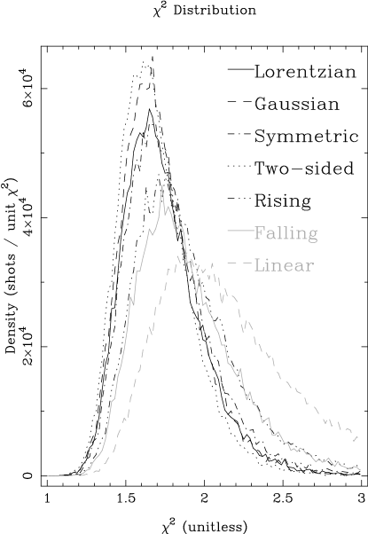
We employ an automated Levenberg-Marquardt fitting routine to compare several template profiles to individual shots and report on the distributions of the resulting parameters. A segment of data equal to the detection window surrounding each event was fit to the following profiles: Lorentzian, Gaussian, symmetric exponential, two sided exponential, rising exponential and falling exponential. All models included a linear background, and a simple linear model was fit to each segment for comparison purposes. $\chi^{2}$ was used as the fit statistic rather than the C-statistic (Cash, 1979) to facilitate comparison between models and shots. The two-sided exponentials and Gaussians provided the lowest $\chi^{2}$ values. The distributions of $\chi^{2}$ for all the models are shown in figure 6, while several shots and their fits to the Gaussian and two-sided exponential models are shown in figure 7. Note that the shots were not separated on the basis of which template fit best — each shot candidate was fit to all template shapes, and the distributions associated with each template shape include all successfully analyzed shot candidates.

Figure 6.— Distributions of reduced $\chi^{2}$. Degrees of freedom varied from 507 to 511 depending on the model. The data intervals around detected shots were fit to a linear background plus the following shot models: A Lorentzian, a Gaussian, symmetric exponential rise and fall, asymmetric (two-sided) exponential rise and fall, rising exponential with a sudden fall, falling exponential with a sudden rise, and no shot.

Figure 7.— Several detected shots and their fits to the Gaussian and two-sided exponential models. Note that in two cases (the upper two panels on the far right) a feature wider than the one that triggered detection was fit. In both cases, however, both models have fit the same feature, which is taken to be a wide shot. In the bottom right panel, a bin near the beginning of the detection window has the same rate as the bin which triggered detection.

As can be seen in figure 7, The fitting routine does not always fit to the feature that triggered detection. This is not surprising: a feature which makes a small contribution to many bins may be more significant than one which makes a larger contribution to fewer bins. It usually does seem to fit the same feature with the different models. Since we were searching for a distribution of shot parameters, it is not disturbing that wider events are sometimes fit — they are the long-time tail of the shot timescale distribution. This seeming deficiency in the fitting process may thus act to ameliorate one of the problems with the detection process — the preference for detecting short, high shots over longer, lower ones with higher significance.

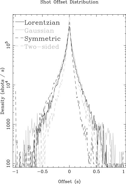
The peak positions were allowed to vary from the initially detected bin during the fitting, but this had little effect on the observed distribution of time separations between shots. This is to be expected since the peak position could not vary outside the detection window, and the initially detected positions cannot be closer together than the detection window — the observed distribution is truncated at the lower end by $t_{d}$, the half-width of the detection window. The peak positions were thus constrained to vary by less than the minimum separation between them, resulting in little effect on the observed distribution of separations. While the distributions of the offset of the fit position from the initially detected position were all sharply peaked at zero, a marked asymmetry was visible in the wings for the symmetric exponential shots (more were shifted to earlier times than later), and a lesser asymmetry with the opposite sense was observed in the two-sided exponentials. This is shown in figure 8.

Figure 8.— Distributions of offsets of the fit positions of the shots from their initially detected position. A marked leftward (toward earlier times) asymmetry is visible in the wings of the distribution for the symmetric exponential shots, and a lesser asymmetry with the opposite sense is visible in the results for the two-sided exponentials. The distribution for two-sided exponentials is narrower than the others.

Figure 9.— Distributions of shot widths. Shots have been characterized by their full width at half maximum. This distribution may not show the shortest shots which triggered the detection routine due to the profile fitting some other feature present in the time surrounding the shot. Due to the bin and interval widths, times shorter than a few tens of milliseconds or longer than a second or two may not be meaningful.

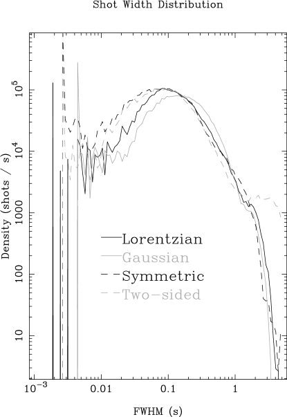
The distribution of shot widths is shown in figure 9. Suggestions of very short bursts of emission (Rothschild et al., 1977) give interest to the number of very short shots. The number of shots with timescales less than 10 ms ranged from 72, when all shots are assumed to be Lorentzian, to 327 when assumed to be symmetric exponential. The shots with the shortest timescales may not have been characterized well by this process — if a shot only occupied a few bins, a greater reduction in $\chi^{2}$ could be obtained by fitting some feature of the background, which might itself be a shot with longer timescale and lower amplitude.

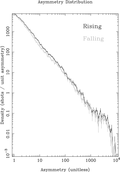
For the two-sided exponentials, the distributions of ratios of fall to rise or rise to fall times (whichever was larger) closely follow similar powerlaws, slope near -1.5. The distribution of shots with a longer rise time is, however, higher than that for longer fall times at all points where the difference is significant, and this is reflected in the count of shots in each category: 18185 slow-rising shots vs. 14611 slow-falling ones. This can be seen in figure 10.

Figure 10.— Distributions of asymmetry ratios for the two-sided exponential model. The larger of the rise or fall time was divided by the other, and the distributions of these ratios plotted. While the slopes are similar, the curve for shots with a slow rise and quicker fall (black) is higher than that for shots with a quick rise and slow fall (gray) everywhere that the difference is significant, i.e. the gray curve is never above the black one by more than the standard deviation.

The distributions of fit heights for the different profiles are similar. This distribution is truncated at the lower end by the requirement to be above some multiple of the local average. These are shown in figure 11.

Figure 11.— Shot height distributions. Heights for 4 fit profiles are shown, along with the heights above the local average of the bins which triggered the detection. This distribution is truncated at small sizes by the detection algorithm.

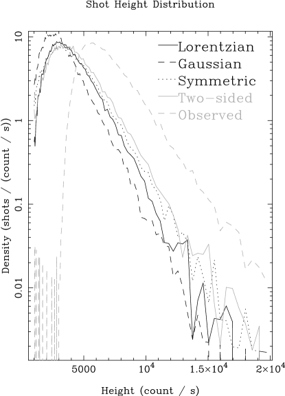
The form of the distribution of directly observed rates for the peak bin (after subtraction of the local average) is similar, but it is displaced upwards in peak intensity when the curves are compared at constant density levels. This is partly due to a selection effect in the detection criteria favoring bins with large positive statistical fluctuations. The separation of the curves, however, is larger than would be expected from Poisson fluctuations alone, suggesting that the profiles used here were not sharp enough to model the peaks of the shots. This interpretation is supported by the differences between the results for the different profiles: The Gaussian profile, with the broadest peak, is displaced furthest toward small heights, while the exponential forms, with the narrowest peaks, are furthest toward high peaks. This seems inconsistent, however, with the fact that the Gaussian profiles had lower typical $\chi^{2}_{\nu}$ values than any other profile but the two-sided exponentials. It may be that the shots have a broad base and a narrow peak, and that the Gaussians tended to fit the base while the exponentials tended to fit the peak. This is also consistent with the fact that the distribution of timescales for the Gaussian profile has more long times than those for the exponential forms.

As we have noted, Gierlinski & Zdziarski (2003) have found 4 powerful millisecond flares in our data sample. Their shot finding algorithm (Gierlinski & Zdziarski, 2003) is coarser than what we have used: $\Delta_{t}=0.125$s, 128 s piecewise constant averaging segment, and threshold defined as $10\sigma_{rms}$. They have estimated that their statistics are consistent with an exponential or log-normal distribution, as extrapolated from lower amplitude shots. This is consistent with our analysis which shows no significant features in the amplitude distribution at large shot heights (see figure 11).

We estimate the energy by the number of photons in the integrated shot profile (the fluence), and observe significant positive correlation in the joint distribution of shot timescale and fluence, shown in figure 12.

Figure 12.— Joint distribution of shot timescales and fluences for two-sided exponential shots. The horizontal axes are shot FWHM (in seconds) and the number of photons in the integrated shot profile. The vertical axis is the density of shots.

4. Coherence Analysis

The ”cross spectrum” of two signals, $f(t)$ and $g(t)$, is defined by:

$$C_{fg}(\omega)=F^{*}(\omega)G(\omega),$$

where $C_{fg}(\omega)$ is the cross spectrum at frequency $\omega$, $F^{*}(\omega)$ is the complex conjugate of the Fourier transform of $f(t)$, and $G(\omega)$ is the Fourier transform of $g(t)$.

The cross spectrum of two measured, binned, signals can be estimated by segmenting them into intervals and averaging the estimated cross spectra from each interval calculated from the discrete Fourier transforms (DFTs) of the signals:

$$<C_{fg,m}>={1\over J}\sum_{j=1}^{J}F^{*}_{m,j}G_{m,j},$$

where $F_{m,j}$ is the DFT of signal $f(t)$ in interval $j$ (out of $J$) in frequency bin $m$. The cross spectrum, like the power spectrum, may also be averaged across adjacent frequencies:

$$<C_{fg,k}>={1\over m_{+}-m_{-}}\sum_{m=m_{-}}^{m_{+}}<C_{fg,m}>.$$

The ”transfer function” $h(t)$ represents $g(t)$ as linearly related to $f(t)$ through the convolution:

$$g(t)=h(t)\star f(t)$$

This relation may not be directly causal; for example, it may be that both $g(t)$ and $f(t)$ are independently, causally, produced from some unobserved ”innovation signal” $i(t)$, each through its own transfer function:

$$f(t)=h_{f}(t)\star i(t),g(t)=h_{g}(t)\star i(t)$$

If innovation signals are applied at more than one location in the system, the observed signals will be the sum of the two innovation signals processed by the transfer functions for their respective locations. If the transfer functions for the different locations are different, their contributions to the cross spectrum will be out of phase and the ”coherence” will be reduced. Note that in the appendix we perform a test of coherence loss when multiple signals are present; we find that the simultaneous presence of different transfer functions would result in decoherence. Coherence is a linear correlation coefficient between the values of the complex Fourier transforms of the two signals as a function of frequency. It measures the consistency of the phase relation (that is, the consistency of $\delta$, the phase of the transfer function) between the two signals over time. The coherence may be calculated as:

$$\gamma^{2}={|<C_{fg}(\omega)>|^{2}\over<|F(\omega)|^{2}><|G(\omega)|^{2}>}$$

Note that the coherence cannot be measured with a single estimate of the cross spectrum, since a single estimate will always be consistent with itself.

The observed value of the coherence is reduced by the presence of measurement noise. Vaughan & Nowak (1997) have derived a correction for this effect, applicable when a good estimate of the PSD of the noise in the signals is available. “Good” here means that the uncertainty in the estimate of the PSD of the noise is significantly less than the PSD of the signal (which is the difference of the PSDs of the data and the noise). Since the main source of measurement noise in light curves used for high-energy astrophysics is counting statistics, of which the expected PSD and distribution thereof are well understood, this correction may usefully be applied here. Low coherence increases the error on phase and coherence estimates (Bendat & Piersol, 1966).

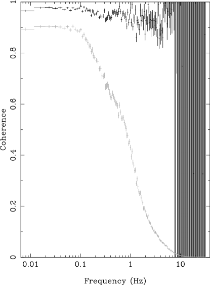
The diagnostic utility of the cross-spectral coherence in timing analyses is often overlooked (Vaughan & Nowak, 1997). When the corrections for noise are applied to the coherence between light curves in different energy bands, the resulting value is consistent with or close to unity. It has been argued that this implies a physically compact location for the source for the variability in all energy bands.

The cross-spectral coherence between the 2–3 keV and 26.5–60 keV bands is shown in figure 13. The coherence is near unity for frequencies below 0.1 Hz and drops to 90% near 10 Hz; this confirms the results obtained by Nowak et al. (1999). At higher frequencies, the power is dominated by noise, and coherence corrections cannot usefully be applied.

Time lag here means that if $f(t)$ and $g(t)$ in the equations above are the soft and hard band light curves, respectively, that $\delta$ is positive. The value of the lag is a function of frequency. The hard band lags in the hard state are shown in figure 14. The time lag shows a power-law dependence upon Fourier frequency, $\tau(f)\propto f^{-0.7}$, with significant deviations from a simple power law; the longest time lag is 0.2 s. This is comparable to the results of Nowak et al. (1999), which obtained the same power-law dependence although with smaller longest time lag (0.05 s). We note that our energy band separation is larger than that of Nowak et al. (1999), so our result confirms the observation that time lags increase with energy band separation.

Figure 13.— Hard state coherence. The coherence between the 2–3 keV and 26.5–60 keV bands in the hard state. The black points have had the corrections for the effects of noise applied, the grey have not.

Figure 14.— Hard band time lags in the hard state. The time lags of the 26.5–60 keV band light curve relative to the 2–3 keV band calculated with the cross-spectrum are plotted as a function of frequency.

5. Summary and Discussion

Our main contribution here is to present the results of an analysis in the time domain in the context of shot noise models, which is complementary to previous analyses in the frequency domain. Our results on Cygnus X-1 hard state coherence and time lags are qualitatively consistent with the results of Nowak et al. (1999) with a much larger and independent data sample. The notion that shot parameters such as timescale and peak rate are distributed — i.e., that the shots are not all the same — is well supported. Models for generation of the shots include inhomogeneity in the orbiting matter (Bao & Ostgaard, 1995), magnetic flares above the disk, with energy released either through reconnection, as in solar flares, or through Comptonization of soft radiation in the disk by the plasma trapped in the flare (Nayakshin & Melia, 1997; Poutanen & Fabian, 1999). Reconnection events in the disk might also give rise to short-term variability and hard emission. Increased emission due to arrival of local density enhancements at the inner edge of the disk has also been suggested (Negoro et al., 1994). Uttley, McHardy, & Vaughan (2005) argue that the simplest explanation of the non-linearity that they find the data supports is that there is a single coherent emitting region with flux from different parts of the emitting region modulated in the same way.

The distribution of timescales constrains thermal Comptonization models for the high-energy emission from this source. The presence of short shots implies that they cannot all have been processed by a large cloud of the sort necessary to produce the observed time lags (up to 0.2 s) between variations in different energy bands (assuming these lags are due to Comptonization). The presence of long shots implies that if they have all been processed by a small corona, some of their width must be intrinsic, and not acquired in the scattering.

There is a distribution of shot lifetimes, so if the width of the shots is due solely to Comptonization time, they must have a distribution of transfer functions. But a distribution of transfer functions should result in reduced coherence, and the observed coherence is high — nearly unity for all frequencies where it can be reliably measured except for the largest energy separations available. The presence of a broad distribution of shot timescales, along with a high cross-spectral coherence, thus supports an intrinsic, dynamical origin for the width of the shots. As mentioned above, Maccarone & Coppi (2002) have shown that shots should be correlated either in arrival times and/or luminosities. Our result of uncorrelated shot arrival times thus implies that shot luminosities are correlated.

Within the shot picture, Feng, Li, & Chen (1999) have found that the shots at higher energy lag behind the shock peaks in the range 2-13 keV and that there is spectral evolution during shots. In case there are non-linear processes focusing towards a shot, these characteristics will have to be shown to evolve. Ours and other studies agree that the characteristics of an apparent shot are intrinsic to the occurrences there. This is a starting point in agreement with the non-linear picture. It is also satisfying that whatever the origin of the shots, their shortest time-scales are on the order of the period that an observer at infinity should see for the innermost circular orbit ($\approx$ 5-7 ms for Cygnus X-1).

Appendix A Test of Coherence Loss when Multiple Signals are Present

In this appendix we show the results of a Monte Carlo experiment which tests for coherence loss when multiple signals are present. While a transfer function that varies in time results in reduced coherence, it was not clear whether this would also be the case when multiple transfer functions were present simultaneously. That is, whether, if the soft light curve were the sum of multiple independent signals:

$$f(t)=\sum_{\{i\}}f_{i}(t),\ \hbox{$\cal F$}[f(t)]=F(\omega)=\sum_{\{i\}}F_{i}(\omega);$$

and the hard state were the sum of the same number of signals, individually coherent with the corresponding soft signal, but with different transfer functions for corresponding signal pairs:

$$G_{i}(\omega)=H_{i}(\omega)F_{i}(\omega),$$

$$g(t)=\sum_{\{i\}}g_{i}(t),\ \hbox{$\cal F$}[g(t)]=G(\omega)=\sum_{\{i\}}G_{i}(\omega)=\sum_{\{i\}}H_{i}(\omega)F_{i}(\omega),$$

$$H_{i}(\omega)\neq H_{j}(\omega),\ i\neq j;$$

coherence would be retained.

In order to investigate this, we performed an experiment with synthetic light curves. Two light curves, $f_{1}$ and $f_{2}$, were created for the “soft” signal, both consisting of a constant plus one-sided exponential shots. Time bins were the same size as in the real data, 1/256 = 0.00390625 s. In each curve, the constant was 1000 count s^-1 and the shots occurred at a rate of 0.5 s^-1, with random positions. In one curve ($f_{1}$), the shots had an $e$-folding time of 0.2 s and a height of 1000 count s^-1, in the other ($f_{2}$) they had 0.02 s and $\sqrt{10}\times 1000=3162$ count s^-1 (these normalizations result in equal total power from each set of shots). “Hard” signals $g_{1}$ and $g_{2}$ were created by delaying $f_{1}$ by 10 time bins and $f_{2}$ by 1 time bin, respectively. These delays are a constant fraction of the width of the shots in the corresponding light curve. The individual transfer functions were thus

$$H_{i}(\omega)=e^{i\omega t_{i}},\ t_{1}=0.0390625\ \hbox{s},\ t_{2}=0.00390625\ \hbox{s}.$$

We used 42 intervals 8 s long to test whether the commingling of two independent and different sets of bursts results in less coherence. Poisson statistics were not imposed on this synthetic data.

These signals were added together and the cross spectrum of $f=f_{1}+f_{2}$ and $g=g_{1}+g_{2}$ was calculated. Since the phase lag of $g_{1}$ relative to $f_{1}$ reaches $\pi$ at a fraction of the Nyquist frequency $F_{c}=F_{N}/10=12.8$ Hz and the cross spectrum routine was not designed with this possibility in mind, the results are only good up to this frequency. At low frequencies (below about 1 Hz) the cross spectrum was coherent, with a time lag slightly below that imposed on $g_{1}$. The coherence dropped at higher frequencies, reaching 50% at $F_{c}$. The time lag started dropping at the same frequency as the coherence, reaching a value slightly higher than that imposed on $g_{2}$. These results are shown in figure 15. It should be noted that the time delays used here are about 1/10 of those observed in the data (to avoid further trouble with phase wrap). This could lessen the loss of coherence compared to what would have been observed in the data were the observed lags due to a distribution of transfer functions: If the phase lags are small, their difference must be also, so the small lags used here will underestimate the loss of coherence. We thus conclude that the simultaneous presence of different transfer functions would result in decoherence.

Figure 15.— Decoherence of simultaneous transfer functions. The time lags and coherence of the cross spectrum of synthetic light curves consisting of two pairs of individually coherent functions are shown. Note that there is no noise applied and no noise correction.

References

- Nowak et al. (1999) Nowak, M. A., Vaughan, B. A., Wilms, J., Dove, J. B., & Begelman, M.C. 1999, ApJ, 510, 874
- Gierlinski & Zdziarski (2003) Gierlinski, M. and Zdziarski, A. 2003, MNRAS, 343, L84
- Rice (1954) Rice, S. O. 1954, in Selected Papers on Noise and Stochastic Processes, ed. N. Wax (New York: Dover Publications), 133
- Terrel (1972) Terrel, N. J. 1972, ApJ, 174, L35
- Miyamoto et al. (1988) Miyamoto, S., Kitamoto, S., Mitsuda, K., & Dotani, T. 1988, Nature, 336, 450
- Lochner et al. (1991) Lochner, J. C., Swank, J. H., & Szymkowiak, A. E. 1991, ApJ, 376, 295
- Belloni & Hasinger (1990) Belloni, T. & Hasinger, G. 1990, A&A, 227, L33
- Negoro et al. (1994) Negoro, H., Miyamoto, S., & Kitamoto, S. 1994, ApJ, 423, L127
- Negoro et al. (1995) Negoro, H., Kitamoto, S., Takeuchi, M., & Mineshige, S. 1995, ApJ, 452, L49
- Takeuchi, Mineshige, & Negoro (1995) Takeuchi, M., Mineshige, S., & Negoro, H. 1995, PASJ, 47, 617
- Maccarone, Coppi, & Poutanen (2000) Maccarone, T. J., Coppi, P. S., & Poutanen, J. 2000, ApJ, 537, L107
- Maccarone & Coppi (2002) Maccarone, T. J. & Coppi, P. S. 2000, MNRAS, 336, 817
- Uttley & McHardy (2001) Uttley, P. & McHardy, I. M. 2001, MNRAS, 323, L26
- Uttley, McHardy, & Vaughan (2005) Uttley, P., McHardy, I. M., & Vaughan, S. 2005, MNRAS, submitted (astro-ph/0502112)
- Cash (1979) Cash, W. 1979, ApJ, 228, 939
- Rothschild et al. (1977) Rothschild, R. E., Boldt, E. A., Holt, S. S., & Serlemitsos, P. J. 1977, ApJ, 213, 818
- Vaughan & Nowak (1997) Vaughan, B. A. & Nowak, M. A. 1997, ApJ, 474, L43
- Bendat & Piersol (1966) Bendat, J. S. & Piersol, A. G. 1966, Measurement and Analysis of Random Data, (New York: John Wiley & Sons)
- Bao & Ostgaard (1995) Bao, G. & Ostgaard, E. 1995, ApJ, 443, 54
- Nayakshin & Melia (1997) Nayakshin, S. & Melia, F. 1997, ApJ, submitted (astro-ph/9710215)
- Poutanen & Fabian (1999) Poutanen, J. & Fabian, A. C. 1999, MNRAS, 306, L31
- Feng, Li, & Chen (1999) Feng, Y. X., Li, T. P., & Chen L. 1999, ApJ, 514, 373
- Feng, Li, & Chen (1999) Feng, Y. X., Li, T. P., & Chen L. 1999, ApJ, 521, 789