CMBR anisotropy: theoretical approaches

Abstract

The version of the cosmological perturbation theory based on exact resolution of energy constraint is developed in accordance with the diffeomorphisms of general relativity in the Dirac Hamiltonian approach. Such exact resolution gives one a possibility to fulfil the Hamiltonian reduction and to explain the “CMBR primordial power spectrum” and other topical problems of modern cosmology by quantization of the energy constraint and quantum cosmological origin of matter.

1. Introduction

One of the basic tools applied for analysis of modern observational data including Cosmological Microwave Background Radiation (CMBR) is the cosmological perturbation theory in general relativity (GR) [1, 2]. The main role in this perturbation theory plays the separation of the cosmological scale factor by the transformation $g_{\mu\nu}=a^{2}(x^{0})\overline{g}_{\mu\nu}$. The similar separation [3, 4, 5, 6] of the homogeneous scale factor $a$ is also fulfilled in the Hamiltonian approach [7, 8] to GR, where $a$ is an invariant evolution parameter in accordance with the Hamiltonian diffeomorphism subgroup $x^{0}\to\widetilde{x}^{0}=\widetilde{x}^{0}(x^{0})$ [9] meaning in fact that the coordinate “time” $x^{0}$ is not observable. In this case, in order to keep the number of variables of GR, such the separation of the scale factor $a$ should be accompanied by the constraint that removes a similar homogeneous variable from the rest spatial metric determinant. Just the separation of homogeneous scale factor from metrics (in contrast with the Dirac Hamiltonian approach [7], where the scale factor $a$ is not taken into account), on the one hand, and the keeping the number of variables of GR (in contrast with the standard perturbation theory [1, 2], where the scale factor $a$ is taken into account twofold), on other hand, gives rise to exact resolution of the energy constraint [5] $\overline{g}^{00}\sqrt{-\overline{g}}/\int d^{3}x\overline{g}^{00}\sqrt{-\overline{g}}=\sqrt{T_{0}^{0}}/\int d^{3}x\sqrt{T_{0}^{0}}$, where $T_{0}^{0}$ is the energy-momentum tensor component in terms of the Lichnerowicz conformal variables [10, 11]. In this paper the perturbation theory based on this exact resolution of the energy constraint in GR is developed and compared with the standard cosmological perturbation theory [1, 2]. The content of the paper is the following. In Section 2, the Hamiltonian approach to GR with the separated cosmological scale is considered. In Section 3, the Hamiltonian perturbation theory is formulated in a finite space-time as an alternative of the cosmological perturbation theory. Two possible descriptions of CMBR are compared in Section 4.

2. The diffeomorphism-invariant Hamiltonian approach to GR

Let us consider the Hilbert - Einstein action of GR

$$S[\varphi_{0}]=\int d^{4}x\sqrt{-g}\left[-\frac{\varphi_{0}^{2}}{6}R(g)+{\cal L}_{(\rm M)}(\varphi_{0}|g,f)\right]$$ (1)

in a space-time with the interval $ds^{2}=g_{\mu\nu}dx^{\mu}dx^{\nu}$, where $\varphi_{0}=\sqrt{3/{8\pi G_{0}}}=\sqrt{3M^{2}_{\rm Planck}/{8\pi}}$ is the Newton coupling constant that scales all masses. The Hamiltonian approach to GR is formulated in a frame of reference given by a geometric interval $g_{\mu\nu}dx^{\mu}dx^{\nu}\equiv\omega_{(0)}\omega_{(0)}-\omega_{(1)}\omega_{(1)}-\omega_{(2)}\omega_{(2)}-\omega_{(3)}\omega_{(3)}$, where $\omega_{(\alpha)}$ are linear differential forms [12] in terms of the Dirac variables [7]

$$\omega_{(0)}=\psi^{6}N_{\rm d}dx^{0},~{}~{}~{}~{}~{}~{}~{}~{}~{}~{}~{}\omega_{(b)}=\psi^{2}{\bf e}_{(b)i}(dx^{i}+N^{i}dx^{0});$$ (2)

here $\psi$ is the spatial metrics determinant variable, triads ${\bf e_{(a)i}}$ form the spatial metrics with $\det|{\bf e}|=1$, $N_{\rm d}$ is the lapse function, and $N^{i}$ is the shift vector.

The forms (2) are invariant with respect to the kinemetric general coordinate transformations $\widetilde{x}^{0}=\widetilde{x}^{0}(x^{0}),\widetilde{x}^{i}=\widetilde{x}^{i}(x^{0},x^{l})$ [9]. This group of diffeomorphisms of the frame (2) means that the coordinate time is not observable. One of the main problems of the Hamiltonian approach to GR is to pick out a diffeomorphism(d)-invariant global variable which can be “evolution parameter”. There is a set of arguments [3, 4, 5, 6, 11] to identify this “evolution parameter” in GR with the cosmological scale factor $a(x_{0})$ introduced by the scale transformation: $F^{(n)}=a^{n}(x_{0})\overline{F}^{(n)}$, where $(n)$ is the conformal weight of any field, including metric components, in particular the lapse function ${N}_{d}=a^{-2}\overline{N}_{d}$ and $\psi^{2}=a\overline{\psi}^{2}\!.$ The logarithm form $\log{\psi^{2}}=F$ of this equation can be presented as a sum $F=\langle F\rangle+[F-\langle F\rangle]$, where $\left\langle{F}\right\rangle\equiv\int d^{3}xF/V_{0}$ identified with $\log a$ ($V_{0}=\int d^{3}x<\infty$ is a finite volume) is the spatial volume “averaging” and $[F-\langle F\rangle]=\overline{F}$ is the orthogonal operation of “deviation” distinguished by the identity

$$\int d^{3}x\log\overline{\psi}^{2}(x^{0},x^{i})=\int d^{3}x\left[\log{\psi^{2}}-\left\langle{\log{\psi^{2}}}\right\rangle\right]\equiv 0.$$ (3)

The transformation of a curvature $\sqrt{-g}R(g)=a^{2}\sqrt{-\overline{g}}R(\overline{g})-6a\partial_{0}\left[{\partial_{0}a}\sqrt{-\overline{g}}~{}\overline{g}^{00}\right]$ converts action (1) into

$$S[\varphi_{0}]=\overline{S}[\varphi]-\int dx^{0}(\partial_{0}\varphi)^{2}\int\frac{d^{3}x}{\overline{N}_{d}}\equiv\int dx^{0}L\equiv\int d^{4}x{\cal L},$$ (4)

here $\overline{S}[\varphi]$ is the action (1) in terms of metrics $\overline{g}$, where $\varphi_{0}$ is replaced by the running scale $\varphi(x^{0})=\varphi_{0}a(x^{0})$ of all masses of the matter fields. The energy constraint ${\delta S[\varphi_{0}]}/{\delta\overline{N_{d}}}=0$ takes the algebraic form [5]:

$$~{}~{}~{}~{}~{}~{}~{}~{}~{}~{}~{}~{}~{}~{}~{}~{}~{}~{}~{}~{}~{}~{}~{}~{}-\frac{\delta\overline{S}[\varphi]}{\delta\overline{N_{d}}}\equiv T^{0}_{0}=\frac{(\partial_{0}\varphi)^{2}}{\overline{N_{d}}^{2}}$$ (5)

where $T^{0}_{0}$ is the local energy density. This equation has exact solution:

$$\left[\frac{d\varphi}{d\zeta}\right]^{2}\equiv\varphi^{\prime 2}={\left\langle\sqrt{{T^{0}_{0}}}\right\rangle}^{2},~{}~{}~{}~{}~{}~{}~{}~{}~{}~{}{\langle(\overline{N_{d}})^{-1}\rangle\overline{N_{d}}}=\frac{{\left\langle\sqrt{{T^{0}_{0}}}\right\rangle}}{\sqrt{{T^{0}_{0}}}},$$ (6)

where

$$\zeta(\varphi_{0}|\varphi)\equiv\int dx^{0}\langle{(\overline{N_{d}})^{-1}}\rangle^{-1}=\pm\int_{\varphi}^{\varphi_{0}}\frac{d\widetilde{\varphi}}{{\langle\sqrt{T_{0}^{0}(\widetilde{\varphi})}\rangle}}$$ (7)

is d-invariant time. This evolution can be treated as the analogy of the Hubble law in the d-invariant formulation of exact GR.

One can construct the Hamiltonian function using the definition of a set of the canonical momenta, including

$$P_{\varphi} = -\frac{\partial L}{\partial(\partial_{0}\varphi)}=2\frac{d\varphi}{dx^{0}}\int\frac{d^{3}x}{\overline{N_{d}}}\equiv 2V_{0}\varphi^{\prime}$$ (8)

$$p_{\psi} = \frac{\partial{\cal L}}{\partial(\partial_{0}\log\overline{\psi})}\equiv-\frac{4\varphi^{2}}{3}\cdot\frac{\partial_{l}(\overline{\psi}^{6}N^{l})-\partial_{0}(\overline{\psi}^{6})}{\overline{\psi}^{6}\overline{N_{d}}},$$ (9)

if the strong constraint $\langle p_{\psi}\rangle=0$ is imposed to be consistent with the identity (3) and to keep the number of variables of GR, otherwise the double counting of the zero-Fourier harmonics of spatial metric determinant [1, 2] does not admit resolution of velocities in terms of momenta (that is the obstacle for the Hamiltonian approach). Now, using solution (6) and definitions (8), (9) one can express action in Hamiltonian form in terms of momenta $P_{\varphi}$ and $P_{F}=[{p_{\psi}},p^{i}_{{(a)}},p_{f}]$

$$S[\varphi_{0}]=\int dx^{0}\left[\int d^{3}x\left(\sum_{F}P_{F}\partial_{0}F+C\right)-P_{\varphi}\partial_{0}\varphi+\frac{P_{\varphi}^{2}-E_{\varphi}^{2}}{4\int dx^{3}(\overline{N_{d}})^{-1}}\right],$$ (10)

where the reduced Hamiltonian function

$$~{}~{}~{}~{}~{}~{}~{}~{}~{}~{}~{}~{}~{}~{}~{}~{}~{}~{}~{}~{}E_{\varphi}=2\int d^{3}x\sqrt{{T^{0}_{0}}}=2V_{0}{\left\langle\sqrt{{T^{0}_{0}}}\right\rangle}$$ (11)

can be treated as the “universe energy” by analogy with the “particle energy” in special relativity (SR), and ${\cal C}=N^{i}{T}^{0}_{i}+C_{0}p_{\psi}+C_{(a)}\partial_{k}{\bf e}^{k}_{(a)}$ is the sum of constraints with the Lagrangian multipliers $N^{i},C_{0},~{}C_{(a)}$ and the energy–momentum tensor components $T^{0}_{i}$; these constraints include the transversality $\partial_{i}{\bf e}^{i}_{(a)}\simeq 0$ and the Dirac minimal space-like surface [7]:

$$~{}~{}~{}~{}~{}~{}~{}~{}~{}~{}~{}~{}~{}~{}{p_{\psi}}\simeq 0~{}~{}~{}~{}\Rightarrow~{}~{}~{}~{}\partial_{j}(\overline{\psi}^{6}{\cal N}^{j})=(\overline{\psi}^{6})^{\prime}~{}~{}~{}~{}~{}({\cal N}^{j}=N^{j}\langle N^{-1}_{d}\rangle).$$ (12)

One can find evolution of all field variables $F(\varphi,x^{i})$ with respect to $\varphi$ by the variation of the “reduced” action obtained as values of the Hamiltonian form of initial action (10) onto the energy constraint $P^{2}_{\varphi}=E^{2}_{\varphi}$ [5]:

$$S[\varphi_{0}]|_{P_{\varphi}=\pm E_{\varphi}}=\int\limits_{\varphi}^{\varphi_{0}}d\widetilde{\varphi}\left\{\int d^{3}x\left[\sum\limits_{F}P_{F}\partial_{\varphi}F+\bar{\cal C}\mp 2\sqrt{T_{0}^{0}(\widetilde{\varphi})}\right]\right\},$$ (13)

where $\bar{\cal C}={\cal C}/\partial_{0}\widetilde{\varphi}$. The reduced Hamiltonian $\sqrt{T_{0}^{0}}$ is Hermitian as the minimal surface constraint (12) removes negative contribution of $p_{\psi}$ from energy density. Thus, the d-invariance gives us the solution of the problem of energy in GR by the Hamiltonian reduction like solution of the similar problem in SR.

The explicit dependence of $T_{0}^{0}$ on $\overline{\psi}$ was given in [10, 11] by extracting the Laplace operator $\hat{\triangle}F\equiv\frac{4\varphi^{2}}{3}\partial_{(b)}\partial_{(b)}F$: $T^{0}_{0}=\overline{\psi}^{7}\hat{\triangle}\overline{\psi}+\sum_{I}\overline{\psi}^{I}\tau_{I}$, where $I$ runs a set of values I=0 (stiff), 4 (radiation), 6 (mass), 8 (curvature), 12 ($\Lambda$-term) in the correspondence with a type of matter field contributions.

3. The diffeomorphism-invariant perturbation theory

Let’s introduce a parametrization of metric $(\overline{N}_{d})^{-1},\overline{\psi}$ through functions $\mu,\nu$

$$~{}~{}~{}~{}~{}~{}~{}~{}~{}~{}\frac{(\overline{N_{d}})^{-1}}{\langle(\overline{N_{d}})^{-1}\rangle}=1+\nu,~{}~{}~{}\overline{\psi}=e^{\mu},~{}~{}~{}\langle\mu\rangle\equiv 0,~{}~{}\langle\nu\rangle\equiv 0$$ (14)

with the zero spatial “averaging” and define partial energy densities $\tau_{I}$ as a sum of the “averaging“ one $\langle\tau_{I}\rangle$ and the “deviation” (3) $\overline{\tau}_{I}=\tau_{I}-\langle\tau_{I}\rangle$ that is orthogonal to the “averaging“ one $\langle\tau_{I}\rangle$, so that the total density takes a form

$$T_{0}^{0}\equiv e^{7\mu}\hat{\triangle}e^{\mu}+\sum\limits_{I}e^{\mu I}\tau_{I},~{}~{}~{}~{}~{}~{}~{}\tau_{I}=\langle\tau_{I}\rangle+\overline{\tau_{I}},~{}~{}~{}\langle\overline{\tau_{I}}\rangle\equiv 0.$$ (15)

The functions $\mu,\nu$ are determined by the constraint (6)

$$1+\nu=\frac{\sqrt{{T^{0}_{0}}}}{\left\langle\sqrt{{T^{0}_{0}}}\right\rangle}\equiv\frac{\sqrt{e^{7\mu}\hat{\triangle}e^{\mu}+\sum\limits_{I}e^{\mu I}\tau_{I}}}{\left\langle\sqrt{e^{7\mu}\hat{\triangle}e^{\mu}+\sum\limits_{I}e^{\mu I}\tau_{I}}\right\rangle}$$ (16)

and the equation ${\delta S[\varphi]}/{\delta\mu}=-\overline{{\cal D}}=\langle{\cal D}\rangle-{\cal D}=0$ of spatial metric variable, where

$$\overline{{\cal D}}=\overline{(1+\nu)^{-1}\left[\sum\limits_{I}Ie^{\mu I}\tau_{I}+7e^{7\mu}\hat{\triangle}\cdot e^{\mu}\right]+e^{\mu}\hat{\triangle}\cdot[e^{7\mu}(1+\nu)^{-1}]}=0.$$ (17)

The Dirac constraint of minimal surface (12) takes the form

$$\partial_{(b)}\left(e^{6\mu}{\cal N}_{(b)}\right)=\partial_{\zeta}(e^{6\mu}).$$ (18)

The d-invariant perturbation theory can be naturally defined as a power series in “deviations” of densities $\overline{\tau}_{I}$ defined in the class of functions with the nonzero Fourier harmonics $\widetilde{\phi}(k)=\int d^{3}x\overline{\phi}(x)e^{ikx}$ satisfying constraint $\langle\phi\rangle=0$:

$$T_{0}^{0} = T_{0}+T_{1}+T_{2}+...,$$ (19)

$$T_{0} = \langle\tau_{(0)}\rangle,$$ (20)

$$T_{1} = \overline{\tau_{(0)}}+(\langle\tau_{(1)}\rangle+\hat{\triangle})\cdot\mu,$$ (21)

$$T_{2} = \mu\left[\overline{\tau_{(1)}}+(\langle\tau_{(2)}\rangle+14\hat{\triangle})\cdot\frac{\mu}{2}\right]+\frac{1}{2}\hat{\triangle}\cdot(\mu^{2}),$$ (22)

where $\tau_{(n)}=\sum_{I}I^{n}\tau_{I}$. In the first order, Eq. (16) takes a form

$$1+\nu=1+\frac{T_{1}}{2T_{0}}=1+\frac{\overline{\tau_{(0)}}+(\langle\tau_{(1)}\rangle+\hat{\triangle})\cdot\mu}{2\langle\tau_{(0)}\rangle}.$$ (23)

The substitution of this value of $\nu$ into the first order of Eq. (17) $\overline{\tau}_{(1)}+(\langle\tau_{(2)}\rangle+14\hat{\triangle})\cdot{\mu}-(\langle\tau_{(1)}\rangle+\hat{\triangle})\cdot\nu=0$ gives $\nu$ and $\mu$ in the form of sum of the Green functions $[D\cdot J](x)=\int d^{3}yD(x-y)J(y)$:

$${\mu} = \frac{1}{14\beta}\left[D_{(+)}\cdot\overline{J_{(+)}}-D_{(-)}\cdot\overline{J_{(-)}}\right],$$ (24)

$${\nu} = \frac{1}{2\beta}\left[(1+\beta)D_{(+)}\cdot\overline{J_{(+)}}-(1-\beta)D_{(-)}\cdot\overline{J_{(-)}}\right],$$ (25)

where $\beta=\sqrt{1+[\langle\tau_{(2)}\rangle-14\langle\tau_{(1)}\rangle]/(7\langle\tau_{(0)}\rangle)}$,

$$\overline{J_{(\pm)}}=7(1\pm\beta)\overline{\tau_{(0)}}-\overline{\tau_{(1)}}$$ (26)

are the local currents, $D_{(\pm)}$ are the Green functions satisfying equations

$$[\pm\hat{m}^{2}_{(\pm)}-\hat{\triangle}]D_{(\pm)}(x,y) = \delta^{3}(x-y),$$ (27)

$$\hat{m}^{2}_{(\pm)} = 14(\beta\pm 1)\langle\tau_{(0)}\rangle\mp\langle\tau_{(1)}\rangle.$$ (28)

The reduced Hamiltonian function (11) after its decomposition (19) takes the form of the current-current interaction

$$E_{\varphi} = 2\int d^{3}x\sqrt{{T^{0}_{0}}}=2V_{0}\sqrt{\langle T_{0}\rangle}\left[1+\frac{\langle T_{2}\rangle}{2\langle T_{0}\rangle}-\frac{\langle T^{2}_{1}\rangle}{8\langle T_{0}\rangle^{2}}+...\right]=$$

$$= 2V_{0}\sqrt{\langle\tau_{(0)}\rangle}\left[1+\frac{1}{28\beta\langle\tau_{(0)}\rangle}\left\langle\left(\overline{J_{(+)}}D_{(+)}\cdot\overline{J_{(+)}}+\overline{J_{(-)}}D_{(-)}\cdot\overline{J_{(-)}}\right)\right\rangle\right].$$

In the case of point mass distribution in a finite volume $V_{0}$ with the zero pressure and the density $\overline{\tau_{(1)}}=\overline{\tau_{(2)}}/6\equiv\sum_{J}M_{J}\left[\delta^{3}(x-y_{J})-\frac{1}{V_{0}}\right]$, solutions (24), (25) take the very significant form:

$$\mu(x) =\sum_{J}\frac{r_{gJ}}{4r_{J}}\left[{\gamma_{1}}e^{-m_{(+)}(z)r_{J}}+(1-\gamma_{1})\cos{m_{(-)}(z)r_{J}}\right],$$ (30)

$$\nu(x) =\sum_{J}\frac{2r_{gJ}}{r_{J}}\left[(1-\gamma_{2})e^{-m_{(+)}(z)r_{J}}+{\gamma_{2}}\cos{m_{(-)}(z)r_{J}}]\right],$$ (31)

where

$${\gamma_{1}}=\frac{1+7\beta}{14\beta},~{}~{}~{}{\gamma_{2}}=\frac{(1-\beta)(7\beta-1)}{16\beta},~{}~{}r_{gJ}=\frac{3M_{J}}{4\pi\varphi^{2}},~{}~{}r_{J}=|x-y_{J}|.$$

The minimal surface (18) gives the shift of the coordinate origin in the process of evolution $\partial_{i}{\cal N}^{i}=6\overline{\mu}^{\prime}$:

$${\cal N}^{i}=\sum_{J}\frac{3r_{gI}^{\prime}}{4}\frac{(x-y_{J})^{i}}{|x-y_{J}|}\left[{\gamma_{1}}e^{-m_{(+)}(z)r_{J}}+(1-\gamma_{1})\cos{m_{(-)}(z)r_{J}}\right].$$ (32)

In the infinite volume limit $\langle\tau_{(n)}\rangle=0$ these solutions take the standard Newtonian form: $\mu=D\cdot\tau_{(0)}$, $\nu=D\cdot[14\tau_{(0)}-\tau_{(1)}]$, ${\cal N}^{i}=0$ (where $\hat{\triangle}D(x)=-\delta^{3}(x)$). However, the isotropic version of Schwarzschild solutions $e^{\mu}=1+\frac{r_{g}}{4r};~{}~{}\frac{e^{7\mu}}{1+\nu}=1-\frac{r_{g}}{4r}$ of equations $\hat{\triangle}e^{\mu}=0,~{}\hat{\triangle}\frac{e^{7\mu}}{1+\nu}=0$ obtained in the infinite volume do not satisfy Eqs. (16), (17) in the presence of cosmological background. Therefore, the exact resolution of these equations does not commute with the infinite-volume limit. The d-invariant analog of the Schwarzschild solution takes the form

$$~{}~{}~{}~{}~{}~{}~{}~{}~{}~{}ds^{2}=a^{2}(\zeta)\left[\frac{e^{12\mu}}{1+\nu}d\zeta^{2}-e^{4\mu}(dx^{i}+{\cal N}^{i}d\zeta)^{2}\right],$$ (33)

where $\mu,\nu,{\cal N}^{i}$ are given by Eqs. (30) – (32) and $\langle\mu\rangle=0$, $\langle\nu\rangle=0$.

The reduced action (13) determines evolution of fields directly in terms of the cosmological scale factor $a=\varphi/\varphi_{0}$ connected with the red shift parameter $z$ by the relation $\varphi=\varphi_{0}/(1+z)$. Therefore, the d-invariant perturbation theory for the reduced Hamiltonian function (3.) converts into the d-invariant cosmological perturbation theory, if all spatial “averagings“ $\langle\tau_{(n)}\rangle$ in (3.) are sums $\langle\tau_{(n)}\rangle=\rho_{(n)}(\varphi)+t^{\rm f}_{(n)}$ of small field parts $t^{\rm f}_{(n)}$ associated with the Standard Model (SM) and the tremendous ($\sim 10^{79}$ GeV) cosmological background $\rho_{(n)}(\varphi)\equiv H_{0}^{2}\varphi_{0}^{2}\Omega_{(n)}$, where $H_{0}$ is the present day value of the Hubble parameter and $\Omega_{(n)}\equiv\sum_{I}{I}^{n}\Omega_{I}(1+z)^{2-I/2}$ here $\Omega_{I}$ is the partial cosmological densities normalized by condition $\Omega_{(0)}=\sum_{I}\Omega_{I}=1$ (recall that the index $I$ runs a set of values I=0 (stiff), 4 (radiation), 6 (mass), 8 (curvature), 12 ($\Lambda$-term) in the correspondence with the type of physical contributions). In the presence of the tremendous cosmological background one can apply the Einstein correspondence principle [5] as the low-energy decomposition of “reduced” action (13) $d\varphi 2\sqrt{\langle\tau_{(0)}\rangle}=d\varphi 2\sqrt{\rho_{(0)}+t^{\rm f}_{(0)}}=d\varphi\left[2\sqrt{\rho_{(0)}}+t^{\rm f}_{(0)}/{\sqrt{\rho_{(0)}}}\right]+...$ over field density $t^{\rm f}_{(0)}$. The first term of these sum $S^{(\pm)}|_{P_{\varphi}=\pm E_{\varphi}}=S^{(\pm)}_{\rm cosmic}+S^{(\pm)}_{\rm field}+\ldots$ is the reduced cosmological action $S^{(\pm)}_{\rm cosmic}=\mp 2V_{0}\int\limits_{\varphi_{I}}^{\varphi_{0}}\!d\varphi\!\sqrt{\rho_{(0)}(\varphi)}$; whereas the second one is the standard field action of GR and SM

$$S^{(\pm)}_{\rm field}=\int\limits_{\eta_{I}}^{\eta_{0}}d\eta\int d^{3}x\left[\sum\limits_{F}P_{F}\partial_{\eta}F+\bar{{\cal C}}-t^{\rm f}_{(0)}\right]$$ (34)

in the space determined by the interval

$$ds^{2}=d\eta^{2}-[e_{(a)i}(dx^{i}+{\cal N}^{i}d\eta]^{2};~{}~{}\partial_{i}e^{i}_{(a)}=0,~{}~{}\partial_{i}{\cal N}^{i}=0$$ (35)

with conformal time $d\eta=d\varphi/\rho_{(0)}^{1/2}$ and running masses $m(\eta)=a(\eta)m_{0}$ [4].

We see that the correspondence principle leads to the theory (34), where the conformal variables and coordinates are identified with observable ones and the cosmic evolution with the evolution of masses. The best fit to the data included high-redshift Type Ia supernovae [13] requires a cosmological constant $\Omega_{\Lambda}=0.7$, $\Omega_{\rm ColdDarkMatter}=0.3$ in the case of the Friedmann “absolute quantities“ of standard cosmology, whereas for “conformal quantities” of the d-invariant approach these data are consistent with the dominance of the stiff state of free scalar field $[z+1]^{-1}|_{({\rm stiff})}(\eta)=\sqrt{1+2H_{0}(\eta-\eta_{0})}$: $\Omega_{\rm Stiff}=0.85\pm 0.15$, $\Omega_{\rm ColdDarkMatter}=0.15\pm 0.10$ [14].

The d-invariant reduction allows us to consider on equal footing the quantum field theories of both particles and universes in the framework of perturbation theory $t^{\rm f}_{(0)}=t_{\rm free}+t_{\rm int}$ extracting the free part $t_{\rm free}=\sum_{p}E_{p}a_{p}^{+}a_{p}^{-}$ with one-particle energies $E_{p}=\sqrt{p^{2}+m^{2}(\eta)}$ [4, 15] and defining Quantum Cosmology as the primary quantization of the energy constraint $P^{2}_{\varphi}-E^{2}_{\varphi}=0$: $\partial^{2}_{\varphi}\Psi+E_{\varphi}^{2}\Psi=0$ and the secondary one: $\Psi=[A^{+}+A^{-}]/({\sqrt{2E_{\varphi}}})$ with the reduced energy $E_{\varphi}=2V_{0}\sqrt{\rho_{(0)}(\varphi)}$, when stable vacua of both universes (u) $B^{-}|0>_{u}=0$ and particles (p) $b_{p}^{-}|0>_{p}=0$ are determined by Bogoliubov’s transformations of “universes” $A^{+}=\alpha_{u}B^{+}\!+\!\beta_{u}^{*}B^{-}$ and particles: $a_{p}^{+}=\alpha_{p}b_{p}^{+}\!+\!\beta_{p}^{*}b_{p}^{-}$. The “vacuum” postulate leads to positive arrow of the time interval (7) $\eta_{\pm}\geq 0$ and its absolute beginning [5]. In the case of the stiff state: $E_{\varphi}=Q/\varphi$, there is an exact solution of Bogoliubov’s equation of a number of “universes” [16]

$${}_{\rm u}\!\!<0|A^{+}A^{-}|0>_{\rm u}=\frac{1}{4Q^{2}-1}\sin^{2}\left[\sqrt{Q^{2}-\frac{1}{4}}~{}~{}\ln\frac{\varphi_{0}}{\varphi_{I}}\right]\not=0,$$ (36)

where the Planck mass $\varphi_{0}=\varphi_{I}\sqrt{1+2H_{I}\eta_{0}}$ belongs to the present-day data $\eta=\eta_{0}$ and $\varphi_{I},H_{I}=\varphi^{\prime}_{I}/\varphi_{I}=Q/(2V_{0}\varphi_{I}^{2})$ are the initial data.

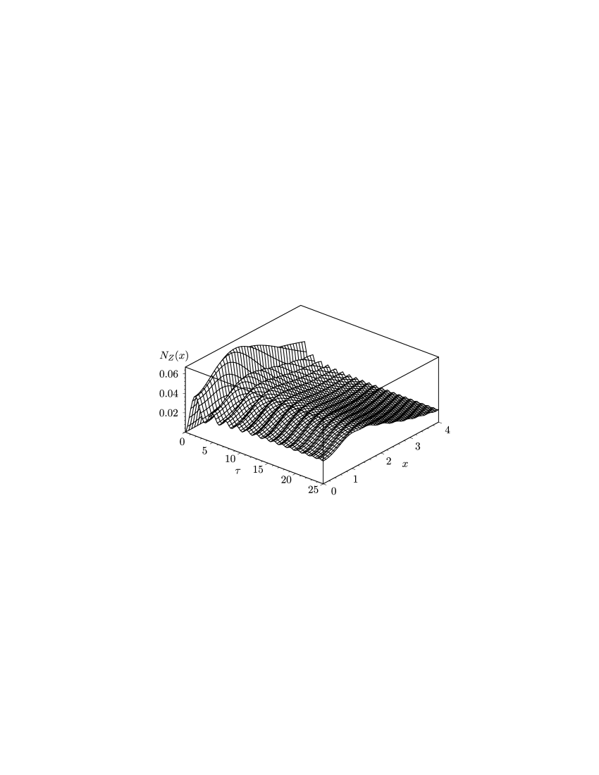
Figure 1: Longitudinal ($N_{Z}(x)$) components of the boson distribution versus the dimensionless time $\tau=2\eta H_{I}$ and the dimensionless momentum $x=q/M_{I}$ at the initial data $M_{I}=H_{I}$ ($\gamma_{v}=1$).

These initial data $\varphi_{I}$ and $H_{I}$ are determined by parameters of matter cosmologically created from the Bogoliubov vacuum in beginning of a universe $\eta\simeq 0$. In the Standard Model (SM), W-, Z- vector bosons have maximal probability of this cosmological creation due to their mass singularity [15]. The uncertainty principle $\triangle E\cdot\triangle\eta\geq 1$ (where $\triangle E=2M_{I},\triangle\eta=1/2H_{I}$) shows us that at the moment of creation of vector bosons their Compton lengths defined by its inverse mass $M^{-1}_{\rm I}=(a_{\rm I}M_{\rm W})^{-1}$ are close to the universe horizon defined in the stiff state as $H_{\rm I}^{-1}=a^{2}_{\rm I}(H_{0})^{-1}$. Equating these quantities $M_{\rm I}=H_{\rm I}$ one can estimate the initial data of the scale factor $a_{\rm I}^{2}=(H_{0}/M_{\rm W})^{2/3}=10^{29}$ and the Hubble parameter $H_{\rm I}=10^{29}H_{0}\sim 1{\rm mm}^{-1}\sim 3K$. Just at this moment there is an effect of intensive cosmological creation of the vector bosons described in [15]; in particular, the distribution functions of the longitudinal vector bosons (see Fig. 1) demonstrate us large contribution of relativistic momenta. Their temperature $T_{c}$ can be estimated from the equation in the kinetic theory for the time of establishment of this temperature $\eta^{-1}_{relaxation}\sim n(T_{c})\times\sigma\sim H$, where $n(T_{c})\sim T_{c}^{3}$ and $\sigma\sim 1/M^{2}$ is the cross-section. This kinetic equation and values of the initial data $M_{\rm I}=H_{\rm I}$ give the temperature of relativistic bosons $T_{c}\sim(M_{\rm I}^{2}H_{\rm I})^{1/3}=(M_{0}^{2}H_{0})^{1/3}\sim 3K$ as a conserved number of cosmic evolution compatible with the Supernova data [14]. We can see that this value surprisingly close to the observed temperature of the CMB radiation $T_{c}=T_{\rm CMB}=2.73~{}{\rm K}$. The primordial mesons before their decays polarize the Dirac fermion vacuum and give the baryon asymmetry frozen by the CP – violation, so that $n_{b}/n_{\gamma}\sim X_{CP}\sim 10^{-9}$, $\Omega_{b}\sim\alpha_{\rm qed}/\sin^{2}\theta_{\rm Weinberg}\sim 0.03$, and $\Omega_{R}\sim 10^{-5}\div 10^{-4}$ [15].

4. Two approaches to descriptions of CMBR fluctuation

Now one can compare the d-invariant perturbation theory (33) with the standard cosmological perturbation theory [1] $ds^{2}=a^{2}(\eta)[(1+\overline{\Phi})d\eta^{2}-(1-\overline{\Psi})(dx^{i}+N^{i}d\eta)^{2}]$, $\overline{\Phi}=\nu-6\mu$ , $\overline{\Psi}=2\mu$, $N^{i}=0$, where the zero-Fourier harmonics of the spatial determinant is taking into account twofold that is an obstruction to the Dirac Hamiltonian method. The d-invariant perturbation theory shows us that, if this double counting is removed, then equations of scalar potential $\mu$ and $\nu$ (see Eqs. (16), (17)) do not contain time derivatives that are responsible for the CMB “primordial power spectrum” in the inflationary model [2]. However, the d-invariant version of the Dirac Hamiltonian approach to GR gives us another possibility to explain the CMBR “spectrum” and other topical problems of cosmology by cosmological creation of the vector bosons considered above. The equations describing the longitudinal vector bosons in SM, in this case, are close to the equations that follows from the Lifshitz perturbation theory and are used, in the inflationary model, for description of the “power primordial spectrum” of the CMB radiation.

The next differences are a nonzero shift vector and the spatial oscillations of the scalar potentials determined by $\hat{m}^{2}_{(-)}$ In the d-invariant version of cosmology [14], the SN data dominance of stiff state $\Omega_{\rm Stiff}\sim 1$ determines the parameter of spatial oscillations $\hat{m}^{2}_{(-)}=\frac{6}{7}H_{0}^{2}[\Omega_{\rm R}(z+1)^{2}+\frac{9}{2}\Omega_{\rm Mass}(z+1)]$. The values of red shift in the recombination epoch $z_{r}\sim 1100$ and the clusterization parameter [17] $r_{\rm clusterization}=\frac{\pi}{\hat{m}_{(-)}}\sim\frac{\pi}{H_{0}\Omega_{R}^{1/2}(1+z_{r})}\sim 130\,{\rm Mpc}$ recently discovered in the researches of large scale periodicity in redshift distribution lead to reasonable value of the radiation-type density $10^{-4}<\Omega_{R}\sim 3\cdot 10^{-3}<5\cdot 10^{-2}$ at the time of this epoch.

5. Conclusions

The diffeomorphism-invariant Hamiltonian approach to GR with an exact solution of energy constraint in a finite volume was applied to formulate the corresponding cosmological perturbation theory. The Hamiltonian cosmological perturbation theory would be considered as the foundation of the standard cosmological perturbation theory [1, 2], if it did not contain the double counting of the scale factor as an obstruction to the Dirac Hamiltonian method. Avoiding this double counting we obtained new Hamiltonian equations. These equations do not contain the time derivatives that are responsible for the “primordial power spectrum” in the inflationary model [2]. However, the Hamiltonian approach to GR gives us another possibility to explain this “spectrum” and other topical problems of cosmology by the cosmological creation of the primordial W-, Z- bosons from vacuum due to their mass singularity, when their Compton length coincides with the universe horizon.

Acknowledgement
The authors are grateful to A. Gusev, A. Efremov, E. Mychelkin, E. Kuraev, L. Lipatov, V. Priezzhev, G. Vereshkov, and S. Vinitsky for fruitful discussions.

References

- [1] E. Lifshitz, Zh. Exp. Teor. Fiz. 16, 587 (1946); J. M. Bardeen, Phys. Rev. D 22, 1882 (1980); H. Kodama, M. Sasaki, Prog. Theor. Phys., N 78, 1 (1984).
- [2] V. F. Mukhanov, H.A. Feldman and R.H. Brandenberger, Phys. Rep. 215, 206 (1992).
- [3] A.M. Khvedelidze, V.V. Papoyan, V.N. Pervushin, Phys. Rev. D 51, 5654 (1995).
- [4] V.N. Pervushin and V.I. Smirichinski, J. Phys. A: Math. Gen. 32, 6191 (1999).
- [5] M. Pawlowski, V.N. Pervushin, Int. J. Mod. Phys. 16, 1715 (2001); [hep-th/0006116].
- [6] B.M. Barbashov, V.N. Pervushin, and D.V. Proskurin, Theoretical and Mathematical Physics 132, 1045 (2002).
- [7] P.A.M. Dirac, Proc. Roy. Soc. A 246, 333 (1958); Phys. Rev. 114, 924 (1959).
- [8] R. Arnowitt, S. Deser and C.W. Misner, Phys. Rev. 117, 1595 (1960).
- [9] A.L. Zelmanov, Dokl. AN USSR 209, 822 (1973).
- [10] A. Lichnerowicz, Journ. Math. Pures and Appl. B 37, 23 (1944).
- [11] J.W. York. (Jr.), Phys. Rev. Lett. 26, 1658 (1971).
- [12] V.A. Fock, Zs. f. Phys. 57, 261 (1929).
- [13] A. G. Riess et al., Astron. J. 116, 1009 (1998) ; S. Perlmutter et al., Astrophys. J. 517, 565 (1999); A. G. Riess et al., Astrophys. J. 560, 49 (2001).
- [14] D.Behnke, D.Blaschke, V.P., D.Proskurin, Phys. Lett. B 530, 20 (2002);[gr-qc/0102039]. D. Behnke, PhD Thesis, Rostock Report MPG-VT-UR 248/04 (2004)
- [15] D. B. Blaschke, S. I. Vinitsky, A. A. Gusev, V .N. Pervushin, and D. V. Proskurin, Physics of Atomic Nuclei 67, 1050 (2004); [hep-ph/0504225].
- [16] V. Pervushin, V. Zinchuk, Talk in XI St.Petersburg School on Theoretical Physics, qr-qc/0504123.
- [17] V.I. Klyatskin, Stochastic Equations, Moscow, Fizmatlit, 2001 (in Russian).
- [18] W. J. Cocke and W. G. Tifft, ApJ. 368, 383 (1991); K. Bajan, P. Flin, W. Godłowski, V. Pervushin, and A. Zorin, Spacetime & Substance 4, 225 (2003).