Measurement of the Energy Release Rate and the Reconnection Rate in Solar Flares

Abstract

By using the method presented by Isobe et al. (2002), the non-dimensional reconnection rate $v_{in}/v_{A}$ has been determined for the impulsive phase of three two-ribbon flares, where $v_{in}$ is the velocity of the reconnection inflow and $v_{A}$ is the Alfvén velocity. The non-dimensional reconnection rate is important to make a constraint on the theoretical models of magnetic reconnection. In order to reduce the uncertainty of the reconnection rate, it is important to determine the energy release rate of the flares from observational data as accurately as possible. To this end, we have carried out one dimensional hydrodynamic simulations of a flare loop and synthesized the count rate detected by the soft X-ray telescope (SXT) aboard Yohkoh satellite. We found that the time derivative of the thermal energy contents in a flare arcade derived from SXT data is smaller than the real energy release rate by a factor of 0.3 – 0.8, depending on the loop length and the energy release rate. The result of simulation is presented in the paper and used to calculate the reconnection rate. We found that reconnection rate is 0.047 for the X2.3 flare on 2000 November 24, 0.015 for the M3.7 flare on 2000 July 14, and 0.071 for the C8.9 flare on 2000 November 16. These values are similar to that derived from the direct observation of the reconnection inflow by Yokoyama et al. (2001), and consistent with the fast reconnection models such as that of Petschek (1964).

1 INTRODUCTION

Magnetic reconnection is now widely believed to be the mechanism of energy release in solar flares. The evidence of magnetic reconnection found by space observations includes the cusp-shaped post flare loop (Tsuneta et al., 1992), the loop top hard X-ray source (Masuda et al., 1994), the reconnection inflow (Yokoyama et al., 2001), downflows above post flare loops (McKenzie & Hudson, 1999; Innes, McKenzie, & Wang, 2003; Asai et al., 2004a), plasmoid ejections (Shibata et al. 1995; Ohyama & Shibata 1997, 1998), etc (see reviews by Shibata 1999; Martens 2003). Magnetic reconnection also plays an important role in various explosive phenomena in astrophysical, space, and laboratory plasmas (Biskamp, 1992; Tajima & Shibata, 1997; Priest & Forbes, 2000).

One important question in the physics of reconnection is what is and what determines the reconnection rate in a plasma with large magnetic Reynolds number such as solar corona. The reconnection rate is the amount of reconnected magnetic flux per unit time and given by $v_{in}B$, where $v_{in}$ is the velocity of reconnection inflow into the diffusion region and $B$ is the magnetic field strength. It is more convenient and physically meaningful to define it in non-dimensional form as $M_{A}=v_{in}/v_{A}$, where $v_{A}$ is the Alfvén velocity. In the following we call this non-dimensional value the reconnection rate. It is important to determine the non-dimensional reconnection rate because theories of magnetic reconnection predict the non-dimensional value.

In classical Sweet-Parker model (Parker, 1957; Sweet, 1958) the reconnection rate $M_{A}$ is given by

$$M_{A}=R_{m}^{-1/2},$$ (1)

where $R_{m}$ is the Magnetic Reynolds number defined by the Alfvén velocity (also called the Lundquist number):

$$R_{m}=\big{(}\frac{v_{A}L}{\eta}\big{)},$$ (2)

$L$ is the length of the reconnecting current sheet and $\eta$ is the magnetic diffusivity. If one consider the classical resistivity by Coulomb collision (Spitzer, 1956), the Magnetic Reynolds number is enormously large ($\sim 10^{14}$) in the solar corona. Therefore the reconnection rate is too small to explain the rapid energy release of solar flares, where the energy release occurs in 10–100 $\tau_{A}$ ($=L/V_{A}$; Alfvén time).

Petschek (1964) considered the effect of MHD slow shocks and proposed a model in which the reconnection rate is about 0.01–0.1 and almost independent of the Magnetic Reynolds number ($M_{A}\propto[\ln R_{m}]^{-1}$). Several MHD simulations have shown that localized resistivity such as anomalous resistivity leads to Petschek type fast reconnection (e.g., Ugai 1986; Scholer 1989; Yokoyama et al. 1994). Erkaev, Semenov, & Jamitzky (2000) also showed that the Petschek regime was realized only when the resistivity is localized, by matching the Petschek-like solution in the inflow region and internal diffusion region solutions. Litvinenko, Forbes, & Priest (1996) examined the reconnection rate in flux-pile-up reconnection and suggested that the reconnection rate is slower than the value of Petschek reconnection by a factor of plasma beta. Nitta (2004) considered the self-similar solution of Petschek type reconnection (i.e., with slow shocks) in free space and found that the reconnection rate is $\sim 0.05$, nearly independent of the plasma beta and, possibly, of the magnetic Reynolds number, too. It is also worth noting that signature of slow mode MHD shocks associated with reconnection was found recently by X-ray observation of a giant arcade formation event (Shiota et al., 2003).

Observational measurement of reconnection rate is not straightforward because measurement of coronal magnetic field strength and inflow velocity is difficult. The only two direct observations of reconnection inflow reported in the literature are those of Yokoyama et al. (2001) and Lin et al. (2005). Yokoyama et al. (2001) found in EUV images two clear patterns approaching toward the reconnection X-point with a velocity about 5 km s^-1. The estimated reconnection rate was 0.001-0.03. Lin et al. (2005) also found a signature of flows toward reconnecting current sheet in a CME-related event and obtained the reconnection rate of 0.01-0.23.

Observations of the chromosphere provide us alternative ways to infer the reconnection rate in the corona. When magnetic reconnection occurs in the corona, the released energy is transported along the magnetic field to the chromosphere by nonthermal high energy particles and/or heat conduction, brightening the footpoints of the reconnected field lines. Therefore successive brightenings in the chromosphere maps the successive magnetic reconnection in the corona. In the standard two-dimensional geometry, the successive reconnection of outer field lines results in the separation of two ribbons (Forbes & Lin, 2000; Lin, 2004), and the (dimensional) reconnection rate, that is also equal to the electric field in the reconnecting current sheet, is given by

$$v_{in}B_{cr}=E_{cs}=v_{foot}B_{foot}.$$ (3)

Here $B_{cr}$ and $B_{foot}$ are the magnetic field strength in the corona and at the footpoint, respectively, $v_{foot}$ is the separation velocity of the footpoints (two ribbons), $E_{cs}$ is the electric field in the current sheet, and $v_{in}B_{cr}$ is the dimensional reconnection rate. Several authors derived $E_{cs}$ (or dimensional reconnection rate) using the observation of chromospheric two ribbons and photospheric magnetograms (e.g., Qiu et al. 2002, 2004, Wang et al. 2003, Fletcher, Pollock & Potts 2003, Asai et al. 2004b).

Isobe et al. (2002) considered equation (3) and the energy release rate to derive the inflow velocity, magnetic field strength in the corona, and hence non-dimensional reconnection rate. They used soft X-ray images taken by the Soft X-ray Telescope (SXT; Tsuneta et al. 1991) aboard Yohkoh satellite to derive the energy release rate and $v_{foot}$, and obtained $M_{A}\approx 0.001-0.01$ for the decay phase of a long duration flare.

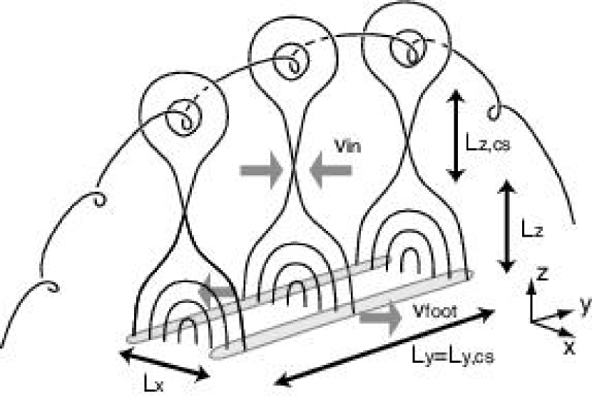
Figure 1: Schematic illustration of the reconnection model of a two ribbon flare.

In this paper we apply the method presented by Isobe et al. (2002) to the impulsive phase of two ribbon flares and determine the reconnection rate $M_{A}$. We analyze three flares with different X-ray flux (one X-class, one M-class, and one C-class) to see whether there is a dependence of $M_{A}$ on the flare class. We selected the flares that exhibit relatively symmetric and regular separation of the flare ribbons, because equation (3) is valid only in the approximately two-dimensional geometry such as shown in figure 1. We should note that it is possible that the successive brightening of the chromosphere is due to the successive magnetic reconnection along the magnetic neutral line, i.e., $y$ direction in figure 1. In this case the velocity of the motion of chromospheric brightening cannot be used to calculate the electric field in the corona. The high electric field (90 V cm^-1) in a complicated C9.0 class flare reported by Qiu et al. (2002) may be due to this effect. Indeed systematic successive reconnection along the neutral line has been observed in giant arcade formation events, where the formation of X-ray loop progress along the neutral line with an apparent velocity of the order of 10 km s^-1 (Isobe, Shibata, & Machida, 2002). Interestingly, similar but faster (50 - 150 km s^-1) evolution of reconnection along neutral line has been reported recently in a M-class flare observed by RHESSI (Grigis & Benz, 2005).

In order to calculate the energy release rate from SXT data as accurately as possible, we have carried out numerical simulations of a flare loop. We synthesized the count rates of different filters of SXT from the simulation result and calculate the thermal energy contents $E_{th}$ that will be observed by the SXT, thus enabling us to convert the time derivative of $E_{th}$ obtained from SXT data to actual energy release rate.

In section 2, the method to determine the reconnection rate is briefly explained. In section 3, we describe the model and results of numerical simulations. In section 4 we describe the observation, data analyses, and results. Discussion and conclusions are given in section 5.

2 HOW TO DETERMINE THE RECONNECTION RATE

In this section we briefly summarize the procedure to calculate the reconnection rate, which is basically the same as that in Isobe et al. (2002) but uses different data set.

We consider the energy release rate $H$ by magnetic reconnection, that is given by the Poynting flux into the diffusion region;

$$H=2\frac{B_{cr}^{2}}{4\pi}v_{in}L_{y,cs}L_{z,cs},$$ (4)

where $L_{z,cs}$ is the vertical length of the reconnecting current sheet, and $L_{y,cs}$ is the length of reconnecting current sheet along the magnetic neutral line. The geometry is illustrated in figure 1. The basic idea is that in equations (3) and (4) the unknown parameters are $B_{cr}$ and $v_{in}$ and the other parameters are obtained from observational data.

As mentioned in the previous section, $v_{foot}$ can be measured from a time sequence of chromospheric images of two ribbons, and $B_{foot}$ can be measured from photospheric magnetograms. In this paper we use 1600 Å  images from the Transition Region and Coronal Explorer (TRACE; Handy et al. 1999) to measure $v_{foot}$, and magnetograms from Michelson Doppler Imager (MDI; Scherrer 1995) aboard the Solar and Heliospheric Observatory (SOHO; Domingo, Flech, & Poland 1995) to measure $B_{foot}$.

Since the reconnecting current sheet is not usually visible, $L_{y,cs}$ and $L_{z,cs}$ are uncertain. We assume $L_{y,cs}$ is equal to the length of flare arcade $L_{y}$. For $L_{z,cs}$, it seems reasonable to assume that in the impulsive phase $L_{z,cs}$ is equals to the height of flare arcade $L_{z}$. This assumption is consistent with MHD simulations (Chen & Shibata, 2000; Shiota et al., 2003) and the inflow observation (Yokoyama et al., 2001). In the decay phase $L_{z,cs}$ may be much larger than $L_{z}$. In this paper we analyze flares near the disk center, therefore we make further assumption that $L_{z}$ is equal to the distance of the footpoints (flare ribbons) $L_{x}$. It is not a bad assumption since many flare loop near the solar limb shows such geometry. Namely, we assume $L_{z,cs}=L_{z}=L_{x}$.

To measure the energy release rate $H$, we use the SXT data. The temperature $T$ and volume emission measure $\rm{\epsilon_{V}}=n^{2}V$ of the flare plasma can be derived from a pair of SXT images with different filters (Hara et al., 1992). Then density $n$ and the thermal energy $E_{th}$ can be calculated by assuming a suitable line-of-sight depth. The energy release rate $H$ can be inferred from the time derivative of the thermal energy $dE_{th}/dt$, although the effect of radiative cooling, conductive cooling and chromospheric evaporation must be considered. In the next section we present the results of numerical simulations to convert the observed $dE_{th}/dt$ to the actual energy release rate $H$.

Finally we calculate the unknown parameters $B_{cr}$ and $v_{in}$ from equations (3) and (4). The Alfvén velocity $v_{A}=B_{cr}/\sqrt{4\pi m_{p}n_{0}}$ ($m_{p}$: proton mass) is calculated using the calculated value of $B_{cr}$ and density $n_{0}$ in the pre-flare phase derived from the SXT images. Thus we obtain the non-dimensional reconnection rate $M_{A}=v_{in}/v_{A}$. To summarize, $B_{cr},v_{in},$ and $M_{A}$ are given by

$$B_{cr}=\frac{2\pi H}{v_{foot}B_{foot}L_{x}L_{y}},$$ (5)

$$v_{in}=\frac{(v_{foot}B_{foot})^{2}L_{x}L_{y}}{2\pi H},$$ (6)

and

$$M_{A}=\frac{v_{in}}{v_{A}}=\frac{(v_{foot}B_{foot})^{3}(L_{x}L_{y})^{2}}{(2\pi H)^{2}}\sqrt{4\pi m_{p}n_{0}},$$ (7)

where the parameters in the right hand sides are observable.

3 NUMERICAL SIMULATION OF A FLARE LOOP

In order to derive the energy release rate $H$ from SXT observations, we have carried out a set of numerical simulations of a flare loop with different loop length and energy input. The effects of Spitzer type thermal conduction, optically thin radiative cooling, and chromospheric evaporation are included. From the results of numerical simulations we calculated the expected count rates for specific filters of the SXT, and then re-calculated the average temperature, emission measure, and hence thermal energy by using the filter ratio method (Hara et al., 1992), as we usually do when we analyze the real observational data. By doing this we can calculate the ratio $\alpha$ of $dE_{th}/dt$ obtained from the SXT data to the actual energy release rate $H$ for various parameters; $\alpha=(dE_{th}/dt)/H$. Then $\alpha$ is used to calculate $H$ from SXT data in section 4. In this paper we consider only the combination of Al 12 $\mu$m (Al12) filter and Be 119 $\mu$m (Be) filter. This pair of Al12 and Be filters has been frequently used in flare observations.

3.1 Basic Assumptions and Equations

As a simple model of a flare loop, we consider a one-dimensional magnetic loop with semi-circular shape and constant cross section. The basic equations are:

$$\frac{\partial\rho}{\partial t}+\frac{\partial}{\partial s}(\rho v) = 0,$$ (8)

$$\frac{\partial\rho v}{\partial t}+\frac{\partial}{\partial s}(\rho v^{2}) = -\rho g_{\parallel}-\frac{\partial P}{\partial s},$$ (9)

$$\frac{\partial e}{\partial t}+\frac{\partial}{\partial s}[(e+P)v] = \frac{\partial}{\partial s}\Big{(}\kappa_{\parallel}\frac{\partial T}{\partial s}\Big{)}-\rho g_{\parallel}v-R+h,$$ (10)

where

$$P=nk_{B}T,\quad e=\frac{1}{2}\rho v^{2}+\frac{P}{\gamma-1}.$$ (11)

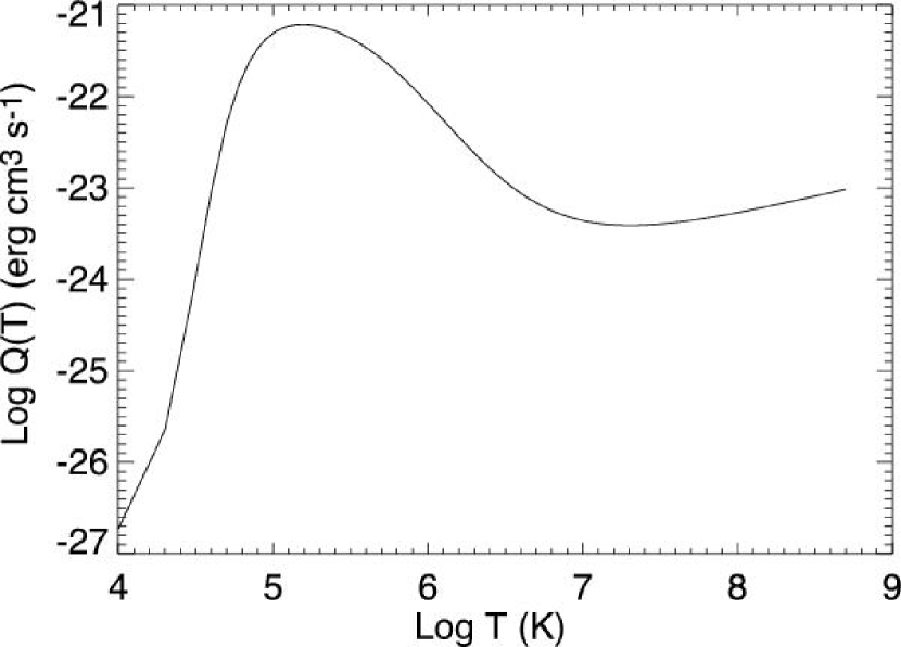
Figure 2: Radiative loss function $Q(T)$.

Here $s$ is the distance along the loop from the photosphere. $\gamma=5/3$ is the ratio of the specific heats. $g_{\parallel}(s)=g_{0}\cos(\pi s/2L)$ is the acceleration by the gravity along the loop; L is the distance from photosphere to the top of the loop. The radiative loss function $R=n^{2}Q(T)$ is chosen to approximate the form for a optically thin plasma with normal solar abundances; $Q(T)$ is shown in figure 2. The thermal conductivity is taken to be of the classical Spitzer form (Spitzer, 1956), that is, $\kappa_{\parallel}=\kappa_{0}T^{5/2}$ erg s^-1 cm^-1 K^-1 and $\kappa_{0}=10^{-6}$ in cgs units. The resulting heat flow is assumed not to be flux-limited. The heating term $h$ is divided into the static heating $h_{s}(s)$ and the flare heating $h_{f}(s,t)$. The static heating term $h_{s}(s)$ is assumed to balance the radiative losses in the initial condition at each point. The second term $h_{f}(s,t)$ is the flare heating, which is described later. The other parameters have their usual meanings.

The basic equations are numerically solved as an initial-boundary value problem. The hydrodynamic parts are solved by modified Lax-Wendroff method (Rubin and Burkstein, 1967) and the heat conduction part is solved by the successive overrelaxation method (e.g., Hirsch 1988). The code has been extensively used for the modeling of solar flares (Hori et al., 1997), X-ray jets (Shimojo et al., 2001) and protostellar flares (Isobe et al., 2003). The detail of the numerical algorithms is described in the Appendix of Hori et al. (1997).

3.2 Initial and Boundary Conditions

The initial condition is hydrostatic atmosphere consisting of isothermal photosphere/chromosphere and hot corona. The temperature distribution in the initial condition is given by

$$T=T_{pho}+\frac{T_{cor}-T_{pho}}{2}\{\tanh\Big{(}\frac{s-s_{tr}}{w_{tr}}\Big{)}+1\},$$ (12)

where $T_{pho}=10^{4}$ K, $T_{cor}=2\times 10^{6}$ K, $s_{tr}=2.8\times 10^{8}$ cm, and $w_{tr}=10^{7}$ cm. The initial density and pressure distributions are calculated from the temperature and gravity distributions by solving hydrostatic equation.

Since we assume that the static heating balances only with the radiative loss, the initial condition is not in strict energy equilibrium. Therefore, even without the flare heating slight decrease of temperature just above the transition region ($s\sim s_{tr}$) and weak evaporation of the chromosphere spontaneously occur due to the conductive heat flux from the hot corona to the cold chromosphere. However, they have negligible effects on the result of simulation because the temperature increase and resultant evaporation by the flare are much stronger. The grid size $\Delta s$ smoothly decreases from $3.2\times 10^{6}$ cm at the photosphere to $2.0\times 10^{7}$ cm around the transition region. In the corona, $\Delta s$ increases from $2.0\times 10^{6}$ cm to $1.0\times 10^{7}$ cm.

We assume symmetry about the loop top and solve only the half of the semi-circular loop, i.e., $0\leq s\leq L$. Mirror boundary condition of the following form is imposed both at $s=0$ and $s=L$. Since our code requires that values of $\rho$, $\rho v$, and $P$ are specified on one grid point at each boundary, we set $\rho_{1}=\rho_{2}$, $\rho_{1}v_{1}=\rho_{2}v_{2}$, and $P_{1}=P_{2}$ for the bottom boundary and $\rho_{N}=\rho_{N-1}$, $\rho_{N}v_{N}=\rho_{N-1}v_{N-1}$, and $P_{N}=P_{N-1}$ for the top boundary. Here the subscripts denote the position of the grid (i.e., $\rho_{i}$ is the density on the ith grid point), and $N$ is the total grid number. The bottom boundary condition does not affect the result of simulation because the gas and energy density near the bottom boundary is much larger than the upper atmosphere and therefore the bottom boundary is not perturbed significantly by the flare heating. We chose the mirror boundary because it is mathematically compatible and the total mass and energy in the simulation domain are conserved.

3.3 Flare Heating

The flare heating function $h_{f}(s,t)$ is of a form of spatially Gaussian,

$$h_{f}(s,t)=\frac{q(t)}{\sqrt{2\pi}\sigma}\exp[-\frac{(s-s_{flr})^{2}}{2\sigma^{2}}]\,\mathrm{(erg}\,\mathrm{cm}^{-3}\,\mathrm{s}^{-1}\mathrm{)}.$$ (13)

We adopt $\sigma=2.0\times 10^{8}$ cm and $s_{flr}=L$, i.e., the flare energy is deposited at the loop top. The total heat flux for the loop $q(t)$ is set to be

$$q(t)=\frac{q_{f}(1-\tanh\{(t-t_{f})/w_{tf}\})}{2}.$$ (14)

We adopt $t_{f}=360$ s and $w_{tf}=1.7$s, because the duration of the impulsive phase is about 6 minutes for all the flares analyzed in this paper. We also performed simulations with uniform heating and footpoint heating to see how the result varies if different form of flare heating is used. The comparison of the different heating models is presented in the Appendix.

3.4 Results of Numerical Simulations

We performed the simulations with different loop length $L$ and heat flux $q_{f}$; $L=2.0,\,3.0,\,3.3$, and $4.0\times 10^{9}\,\rm{cm}$ and $q_{f}=0.4,\,0.8,\,4,\,8,\,40,\,80$, and $243\,\times 10^{8}\,\rm{erg}\,\rm{s}^{-1}\,\rm{cm}^{-2}$. The other parameters were kept constant. In the following we show the result of the run with $L=3.3\times 10^{9}\,\rm{cm}$ and $q_{f}=8.0\times 10^{8}\,\rm{erg}\,\rm{s}^{-1}\,\rm{cm}^{-2}$.

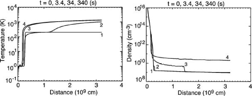
Figure 3: Temperature and density distribution of the simulation result with typical parameters (see the text). The labels 1, 2, 3, and 4 in the figure indicate the time; $t=$ 0, 3.4, 34, and 340 s, respectively.

Figure 3 shows the temperature and density distributions at $t=$ 0, 3.4, 34, and 340 s. Since the flare energy is injected at the loop top, the temperature at the loop top rises rapidly, and the energy is transported by heat conduction. The conduction front is seen near $s=1.2\times 10^{9}$ cm at $t=3.4$. When the conduction front reaches to the chromosphere, the cold and dense plasma is heated to the flare temperature, and the resultant high pressure drives the upward flows, i.e., chromospheric evaporation ($t=34$ s). The evaporation plasma fills the flare loop and increases the soft X-ray emission ($t=340$ s).

From the temperature and density distributions in the result of simulation, the counts of signal that will be detected by SXT can be calculated by

$$I_{j}=\sum_{i=1}^{N}f_{j}(T_{i})n_{i}^{2}\Delta s_{i},$$ (15)

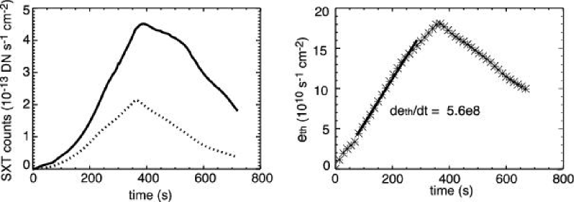
Figure 4: Left: Synthesized light curves. The solid and dashed lines are the light curves of Thick Al. and Be filters, respectively. They must be multiplied by $3.2\times 10^{16}$ to obtain the value in DN s^-1 pixel^-1 for full resolution image. Right: Temporal variation of $e_{th}$, the thermal energy per unit area derived by the SXT filter ratio method. The solid line is the least square fitting of the impulsive phase.

where $f_{j}$ is the response function of the filter $j$, $I_{j}$ is the count rate of SXT with filter $j$, $i$ denotes the grid number, and $\Delta s_{i}$ is the spacing of the $i$th grid. The left panel of figure 4 shows the synthesized SXT count rates for Al12 filter ($I_{Al}$: solid line) and for Be filter ($I_{Be}$: dashed line). Note that the unit is DN (data number) per second per unit area, where the area is that on the solar surface. Since one pixel of the full resolution image of SXT corresponds to $2.45$ arcsec $\approx 1.8\times 10^{8}$ cm on the solar surface, to obtain the count rate in DN s^-1 pixel^-1, the values in figure 4 must be multiplied by $3.2\times 10^{16}$.

From $I_{Al}$ and $I_{Be}$, the average temperature $T$ and emission measure $\epsilon_{L}=n^{2}L$ in the flare loop can be calculated by the filter ratio method (Hara et al. 1992). Here $\epsilon_{L}$ is the emission measure of the loop with a cross section of 1 cm². The thermal energy of the loop is given by

$$e_{th}=\frac{2nk_{B}T}{\gamma-1}L=3\sqrt{\epsilon_{L}L}k_{B}T\,\mathrm{(erg}\,\mathrm{cm}^{-2}\mathrm{)}.$$ (16)

The total thermal energy $E_{th}$ is then given by $E_{th}=e_{th}S$, where $S$ is the cross section of the flare loop(s) which is arbitrary in the simulation. Finally we obtain the ratio $\alpha$;

$$\alpha=\frac{dE_{th}/dt}{H}=\frac{de_{th}/dt}{q_{f}},$$ (17)

where $q_{f}$ is the input heat flux of the flare. Note that the thermal energy calculated in this way is that of the high temperature plasma, because the SXT sees only the hot coronal plasma ($T\geq 2\times 10^{6}$ K). The temporal variation of $e_{th}$ is shown in the right panel of figure 4. We defined the impulsive phase as $0.2t_{flr}\leq 0.8t_{flr}$ and calculated the average gradient of the $e_{th}(t)$ in the impulsive phase by the least square fitting. The solid line in the right panel of figure 4 shows the result of least square fitting that yields $de_{th}/dt=5.6\times 10^{8}$ erg s^-1 cm^-2. Since the input heat flux in this simulation is $8.0\times 10^{8}$ erg s^-1 cm^-2, $\alpha=0.7$ in this case.

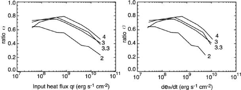
Figure 5: The ratio $\alpha=(de_{th}/dt)/q_{f}$ plotted against $q_{f}$ (left) and $de_{th}/dt$ (right). The numbers in the figure indicate the loop length ($10^{9}$ cm).

We calculated $\alpha$ for all the other parameters by the same procedure. The result is shown in figure 5. The left and right panels plot $\alpha$ against input heat flux and $de_{th}/dt$, respectively. The numbers in the figure indicate the loop length. Although there are some exceptions, basically larger heat flux or shorter loop length result in smaller $\alpha$. We interpret this tendency as follows. When the heat flux is larger or the loop length is shorter, the conductive flux into the chromosphere is larger, and hence the conductive cooling is more effective. Moreover, larger conductive flux leads to stronger chromospheric evaporation and larger density in the corona. Therefore radiative cooling is also effective in such cases. In the following analyses we use $\alpha$ to calculate the real energy release rate $H$ from $dE_{th}/dt$ obtained from SXT images.

4 RECONNECTION RATE

Using the method described in section 2 and the result of the simulation presented in section 3, we have analyzed three flares: an X2.3 class flare on 2000 November 24, an M3.7 class flare on 2000 July 14, and a C8.9 class flare on 2000 November 16. These flares were selected because (1) they show relatively symmetric expansion of two ribbons in TRACE 1600 Å  image, (2) the SXT data taken with Al12 and Be filters are available for the impulsive phases, (3) magnetograms from SOHO/MDI are available, and (4) the size ($\sim 4\times 10^{9}$ cm) and the duration of the impulsive phase ($\sim 6$ min) are similar.

4.1 X2.3 Flare on 2000 November 24

This flare is one of the three X-class homologous flares occurred on 2000 November 24 in NOAA 9236. This active region produced many homologous flares and coronal mass ejections and has been extensively studied (e.g., Nitta & Hudson 2001; Zhang & Wang 2002; Zhang, Solanki, & Wang 2003; Moon et al. 2003; Takasaki et al. 2004) A quantitative analysis of the ribbon separation and hard X-ray emission of the homologous flares was presented by Takasaki et al. (2004).

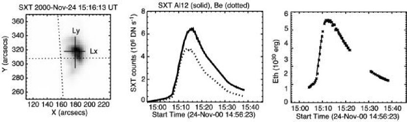
Figure 6: Left: SXT image of the X2.3 flare on 2000 Nov. 24. The image is negative. The solid lines indicate $L_{x}$ (shorter line) and $L_{y}$ (longer line) measured by eyes. Middle: Light curves of the Al 12 filter images (solid line) and Be filter images (dotted line). Right: Temporal variation of thermal energy $E_{th}$. The solid line indicates the least square fitting of the impulsive phase, that yields $dE_{th}/dt=1.6\times 10^{28}$ erg s^-1.

The SXT image near the peak is shown in figure 6 (left panel). The solid lines indicate $L_{x}=2.2\times 10^{9}$ cm and $L_{y}=3.5\times 10^{9}$ cm measured by eyes. The effect of projection on the plain of sky is corrected. Since the X-ray arcade grows with time and the arcade and flare ribbons are not exactly symmetric, the measured $L_{x}$ and $L_{y}$ are rough estimates. In this paper we consider the spatial and temporal average of the reconnection rate, so we use above values of $L_{x}$ and $L_{y}$ as the representative values to calculate the reconnection rate. In order to study the spatial and temporal variation of the reconnection rate, the size and other parameters must be measured more carefully considering the complicated and asymmetric structure.

The middle panel of figure 6 shows the temporal variation of the intensity integrated over the flare arcade. The solid and dotted lines are for Al12 and Be filter images, respectively. Since the SXT instrument cannot obtain two images with different filters simultaneously, we calculate the intensity of Al12 filter images at the same time of Be filter images by linear interpolation, and then calculate the temperature $T$ and the volume emission measure $\epsilon_{V}=n^{2}V$ by the filter ratio method. We assume that the line of light length of the arcade ($\sim$ height of the arcade) is equals to $L_{x}$, the distance between the footpoints. This assumption is justified because we empirically know from the observations of limb flares that the height of a flare arcade is approximately equals to the distance between its footpoints. We also assume the volume filling factor $f=0.1$; $V=L_{x}^{2}L_{y}f$. This is also from our empirical knowledge that inner part of a flare arcade usually looks like a void. With these assumptions the thermal energy of the flare arcade is given by

$$E_{th}=3nk_{B}TV=3k_{B}T\sqrt{\epsilon_{V}V}.$$ (18)

The right panel of figure 6 shows the temporal variation of $E_{th}$. The solid line is the least square fitting in the impulsive phase. From the gradient of the solid line we obtain $dE_{th}/dt=1.6\times 10^{28}$ erg s^-1.

We use the result of numerical simulation to calculate the real energy release rate $H$ from $dE_{th}/dt$. In order to compare with the one-dimensional numerical simulation, we need to know the energy release rate per unit area $de_{th}/dt$. To obtain this, we simply divide total energy release rate $dE_{th}/dt$ by the apparent area of the flare arcade $L_{x}L_{y}$; $de_{th}/dt=(dE_{th}/dt)/(L_{x}L_{y})=2.0\times 10^{9}$ erg s^-1 cm^-2. From the assumed geometry we estimate that the loop length (distance from footpoint to looptop) is about $1.3L_{x}\approx 3\times 10^{9}$ cm. Then from figure 5 we see that $\alpha=0.6$ for this flare. Thus we obtain $H=(dE_{th}/dt)/\alpha=2.7\times 10^{28}$ erg s^-1. These parameters are summarized in table 1.

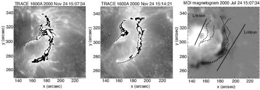
Figure 7: Left and middle: TRACE 1600 Å  images of the X2.3 flare at $t_{1}=$15:07:34 and $t_{2}=$15:14:21. The dashed lines indicate the outer edge of the flare ribbons at each time. Right: MDI magnetogram of the same field of view. The dashed lines indicate the locations of the outer edges of the ribbons both at $t=t_{1}$ and $t_{2}$. The solid lines in the left panel indicate the length of the ribbon $L_{ribbon}$ for the east (left) and west (right) ribbons.

Next step is to measure the separation velocity $v_{foot}$ and field strength $B_{foot}$ of the flare ribbons. Although the three flares analyzed in this paper have relatively symmetric and simple ribbons, $v_{foot}$ and $B_{foot}$ are different at the different position on the ribbons. Since we are interested in the average values, $v_{foot}$ and $B_{foot}$ are measured by following procedure. (1) Two TRACE 1600 Å  images, one near the beginning of the impulsive phase and one just before the end of the impulsive phase, are selected. (2) The MDI magnetogram at the nearest time is selected and coaligned with the TRACE 1600 Å  images. The coalignment is done by taking cross-correlation of the TRACE white-light image and the MDI continuum image. (3) The outer edges of the ribbons in the TRACE 1600 Å  images are defined by visual inspection of the images (see figure 7). (4) The magnetic flux $\phi=\int BdA$, where $A$ is the area swept by the outer edge of the flare ribbons, is calculated from the coaligned magnetogram. We assume that magnetic field is vertical at the photosphere, and correct the effect of projection. The average field strength $B_{foot}$ is given by $B_{foot}=\phi/A$. (5) The (average) separation velocity $v_{foot}$ is calculated by

$$v_{foot}=\frac{A}{L_{ribbon}(t_{2}-t_{1})},$$ (19)

where $L_{ribbon}$ is the length of the ribbon, and $t_{2}$ and $t_{1}$ are the times of the TRACE images ($t_{2}>t_{1}$). This procedure is applied to each ribbon separately. We use the average $B_{foot}$ and $v_{foot}$ of the two ribbons to calculate the reconnection rate.

Figure 7 shows the TRACE 1600 Å  images near the beginning ($t_{1}=$15:07:34 UT) and end ($t_{2}=$15:14:21 UT) of the impulsive phase, as well as the coaligned MDI magnetogram. The dashed lines indicate the outer edges of the ribbons. The magnetic flux $\phi$ are calculated by summing up the flux of all the pixels between the ribbon edges at $t=t_{1}$ and $t=t_{2}$. The solid lines beside the locations of the ribbons (dashed lines) indicate $L_{ribbon}$ for the east (left on the image) ribbon and the west (right on the image) ribbon.

Table 2 shows $\phi,L_{ribbon},B_{foot}$ and $v_{foot}$ for the east and west ribbons and their average values. Effect of the projection has been corrected. It should be noted that the values of the magnetic flux $\phi$ of the two ribbons are not equal. Such flux unbalance has also been reported by Fletcher & Hudson (2001). Finally, the $B_{cr}$, $v_{in}$, $M_{A}$, and $E_{cs}$ are calculated by equations (3), (5), (6), and (7) using the average values of $B_{foot}$ and $v_{in}$ as well as $H,L_{x},L_{y},$ and $n_{0}$ derived from the SXT data. The results are shown in table 1. We obtained $B_{c}=41$ G, $v_{in}=1.3\times 10^{7}$ cm s^-1, $M_{A}=0.047$, and $E_{cs}=539$ V m^-1.

4.2 M3.7 Flare on 2000 July 14

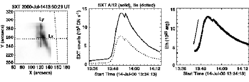
Figure 8: The same figure as figure 6 for the M3.7 flare on 2000 Jul. 14. $dE_{th}/dt=3.5\times 10^{27}$ erg s^-1.

This flare occurred in NOAA 9077 at 13:45 UT on 2000 July 14, the same day as the famous 2000 Bastille Day flare but in the different active region. The SXT image, light curves, and the temporal variation of $E_{th}$ are shown in figure 8 in the same manner as figure 6. Since the solid line showing the least square fitting of $E_{th}(t)$ is almost invisible, a line with the same slope ($=dE_{th}/dt$) is also shown in the figure.

Following the same procedure as the 2000 Nov 24 flare, we obtained $L_{x}=1.5\times 10^{9}$ cm, $L_{y}=4.2\times 10^{9}$ cm, and $dE_{th}/dt=3.5\times 10^{27}$ erg s^-1. The ratio $\alpha$ is taken from figure 5. The loop length is $1.3L_{x}\approx 2\times 10^{9}$ cm and the energy release rate per unit area is $(de_{th}/dt)\approx 5.6\times 10^{8}$ erg s^-1 cm^-2, hence $\alpha=0.55$ and $H=(dE_{th}/dt)/\alpha=6.4\times 10^{28}$ erg s^-1.

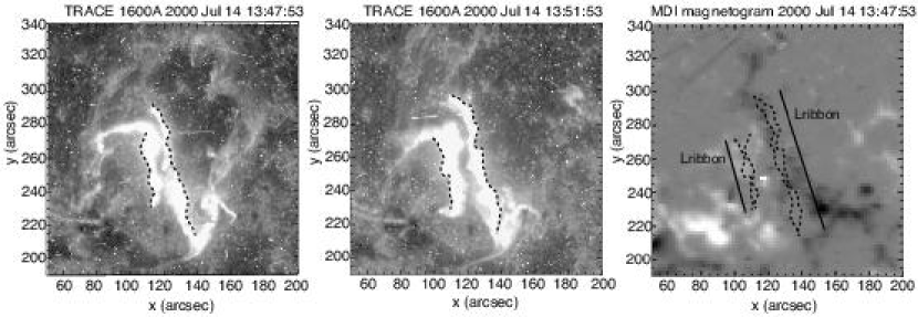
Figure 9: The same figure as figure 7 for the M3.7 flare on 2000 Jul. 14.

The TRACE 1600 Å  images and magnetogram of the flare are shown in figure 9, and the values of $\phi,B_{foot},$ and $v_{foot}$ are shown in table 3. When we define the outer edge of the flare ribbons to calculate the magnetic flux, the upper part of the east (left) ribbon and the lower part of the west (right) ribbon that exhibit irregular shape are neglected because they seem to deviate from the standard two-dimensional geometry. Nevertheless the unbalance of $\phi$ is small. Finally we obtain $B_{cr}=44$ G, $v_{in}=3.2\times 10^{6}$ cm s^-1, $M_{A}=0.015,$ and $E_{cs}=143$ V m^-1. Other parameters are shown in table 1.

4.3 C8.9 Flare on 2000 November 16

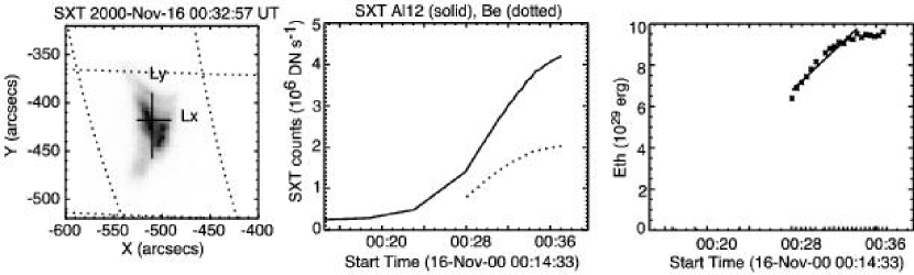
Figure 10: The same figure as figure 6 for the C8.9 flare on 2000 Nov. 16. $dE_{th}/dt=1.2\times 10^{27}$ erg s^-1.

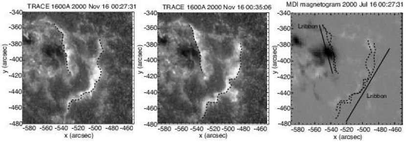
Figure 11: The same figure as figure 7 for the C8.9 flare on 2000 Nov. 16.

This flare occurred at 00:20 UT on 2000 November 16 in NOAA 9231. The SXT image, light curves, and the temporal variation of $E_{th}$ are shown in figure 10, and the TRACE 1600 Å  images and the MDI magnetogram are shown in figure 11, in the same manner as previous two flares. From the SXT data we obtain $L_{x}=3.1\times 10^{9}$ cm, $L_{y}=5.2\times 10^{9}$ cm, and $dE_{th}/dt=1.2\times 10^{27}$ erg s^-1. The loop length $1.3L_{x}\approx 4.0\times 10^{9}$ cm and the energy release rate per unit area $de_{th}/dt=7.4\times 10^{7}$ erg cm^-2, hence from figure 5 $\alpha=0.65$ and $H=1.9\times 10^{27}$ erg s^-1. Measurement of $\phi,B_{foot},$ and $v_{foot}$ are also done in the same manner. The results are shown in table 4. Finally we obtain $B_{cr}=11$ (G), $v_{in}=6.7\times 10^{6}$ cm s^-1, $M_{A}=0.071,$ and $E_{cs}=70$ V m^-1. Other parameters are shown in table 1.

4.4 Estimate of Uncertainty

It is difficult to estimate the uncertainties of the obtained values of $M_{A},v_{in},$ and $B_{cr}$, because there are many factors that cause the uncertainty, though our method includes fewer assumptions than previous studies. Here we try to make a rough estimation of the uncertainty. First of all we should note that the obtained reconnection rate is the spatial and temporal average in the impulsive phase. Actually the reconnection process is often noisy and intermittent, which is clear from the highly variable, bursty light curves of nonthermal emissions such as hard X-ray and microwave. Careful examinations of the flare ribbons also suggest that the reconnection rate is noisy both in space and in time (Saba, Gaeng, & Tarbell, 2002; Fletcher, Pollock, & Potts, 2003). Therefore each elementary process of reconnection in the flares can be faster than the average value obtained here.

The thermal energy contents of the flare calculated in this study is consistent with previous works (e.g., Ohyama & Shibata 1997, 1998; Emslie et al. 2004). However, we wish to measure the energy release rate $H$ as accurately as possible, because uncertainty in $H$ has significant influence on the calculated value of the reconnection rate. The possible source of the uncertainty in the energy release rate $H$ is: (1) temperature and emission measure diagnostics by SXT, (2) error in the conversion from $dE_{th}/dt$ (measured from SXT data) to $H$ using the results of the numerical simulations, and (3) measurement of the volume $V$. As for (1), the statistical error due to the photon noise is negligible. As for (2), $\alpha$ may depends on the detail of the simulation model such as the initial condition, location of the flare heating, etc. We performed simulations with different parameters and found that the detail of initial condition does not have significant consequence in the result when the total energy of the flare is much larger than the initial thermal energy contents of the loop. On the other hand, simulations with different heating locations indicate that if most of the flare energy is deposited deep in the chromosphere, $\alpha$ parameter may be significantly smaller. However, within the range of reasonable parameters the uncertainty in the ratio $\alpha$ is about $\pm 20\%$. The result of simulations with different heating locations is presented in the Appendix.

Probably the largest uncertainty in $H$ comes from (3), the uncertainty of the volume. We made assumptions that the line of sight length of an arcade is equal to its footpoint distance $L_{x}$ and a volume filling factor of 0.1. We cannot tell precisely how good these assumptions are, but we empirically know that the assumption of the geometry (i.e., $L_{z}=L_{x}$) is not a bad assumption, and probably the uncertainty is a factor of 2 at most. An alternative way to estimate the line of sight length may be to use the scaling law that relates the loop length (from apex to footpoint) to the rise time, decay time, and temperature of the flare (Metcalf & Fisher, 1996). We applied this scaling law by Metcalf & Fisher (1996) to the flares analyzed in this paper and obtained the loop length of $1.3\times 10^{9}$ cm, $1.3\times 10^{9}$ cm, and $2.6\times 10^{9}$ cm for the X2.3, M3.7, and C8.9 flares, respectively. These values are 1.5-2.2 times smaller that our assumption that the loop length is equal to $1.3L_{x}$. This also supports that the uncertainty of the line of sight length is about a factor of 2.

The uncertainty of the volume filling factor is more difficult to address, but it seems that an uncertainty of a factor of 5 is reasonable. The upper limit comes again from our empirical knowledge of the geometry of flare loops/arcades, and the lower limit comes from that if the filling factor is so small as 0.01, the number density of the plasma in the loops must be unreasonably large ($\sim 10^{13}$ cm^-3).

Combining the uncertainties of the line of sight length and the filling factor, we conclude that the uncertainty of the volume is a factor of 10. From equation (18) we see that the thermal energy is proportional to $\sqrt{V}$, hence the uncertainty in $E_{th}$ is about a factor of $\sqrt{10}$. Combining (1)–(3), we estimate that uncertainty in $H$ is about a factor of 4.

About the measurement of $B_{foot}$ and $v_{foot}$, There must be errors that come from the alignment of the TRACE 1600 Å  ribbons and MDI magnetogram. The alignment of the TRACE images and MDI magnetograms has been done by taking the cross correlation of the white light images of TRACE and the continuum images of MDI. We found that the correlation between the two images was good in all the flares and estimated the error is about 1 MDI pixel. This is consistent with the work by Fletcher & Hudson (2001) who used the same method for the coalignment of TRACE 1600 Å  images and MDI magnetogram. The magnetic flux $\phi$ measured by shifting the magnetogram by 1 pixel yield the uncertainty of a few $\%$.

However, the unbalance of $\phi$ between the two ribbons indicates that there must be other source of uncertainty. As discussed by Fletcher & Hudson (2001) in detail, the uncertainty may come from: (1) the inclination of the photospheric field (2) not all the flux below the illuminated ribbons are involved in the reconnection event (3) uncertainty of the sensitivity of MDI magnetogram, especially to the small scale, and so on. Although we do not know which factor is dominant, for the present purpose, it is enough to roughly estimate the uncertainty of the value of product $B_{foot}v_{foot}$. In the three flares analyzed in this paper, the largest difference of $E_{cs}=B_{foot}v_{foot}$ between two ribbons is about a factor of 2.4 (2000 Nov 24 flare). If we adopt the values for the east and west ribbons as the upper and lower limits, the uncertainty of $B_{foot}v_{foot}$ may be considered to be a factor of $\sqrt{2.4}\approx 1.5$;

$$\log_{10}(B_{foot}v_{foot})=\log_{10}(B_{foot}v_{foot})_{\rm{average}}\pm\log_{10}1.5\,\,(\approx 0.2).$$ (20)

From equations (5) – (7), we see

$$B_{cr}\propto H^{1}(B_{foot}v_{foot})^{-1}$$

$$v_{in}\propto H^{-1}(B_{foot}v_{foot})^{2}$$

$$M_{A}\propto H^{-2}(B_{foot}v_{foot})^{-3}.$$

Therefore, the estimated uncertainties are $\pm\log_{10}(4^{1}\times 1.5^{1})\approx 0.8$ for $\log_{10}B_{cr}$, $\pm\log_{10}(4^{1}\times 1.5^{2})\approx 1.0$ for $\log_{10}v_{in}$, and $\pm\log_{10}(4^{2}\times 1.5^{3})\approx 1.7$ for $\log_{10}M_{A}$.

For the uncertainty of the reconnection rate $M_{A}$, the uncertainty of the preflare density $n_{0}$ should be also taken into account. The largest uncertainty of $n_{0}$ comes from the uncertainty of the line of sight length $l$. However, since $v_{A}\propto n_{0}^{-1/2}\propto l^{1/4}$, the uncertainty of the preflare density can be neglected.

5 DISCUSSION

By considering the separation velocity of the flare ribbons and energy release rate, we have obtained dimensionless reconnection rate $M_{A}$ as well as the inflow speed $v_{in}$ and magnetic field strength $B_{cr}$ in the corona for the impulsive phases of three flares. The obtained values of reconnection rate (0.015-0.071) are consistent with the fast reconnection models (e.g., Petschek 1964). In other words we have confirmed that the motion of flare ribbons and the energetics of the flares are consistent with the standard scenario that the magnetic energy is released via fast magnetic reconnection. Furthermore, it seems that the large energy release rate $H$ and electric field $E_{cs}$ in the X-class flare are simply due to the large magnetic field strength and Alfvén velocity in the corona.

Previously several authors tried to estimate the non-dimensional reconnection rate from observational data (e.g., Dere 1996; Tsuneta 1996; Ohyama & Shibata 1997, 1998; Forbes & Lin 2000) and obtained similar values. Our method has advantages to previous studies that it requires fewer assumptions and that the inflow velocity and magnetic field strength in the corona are also obtained (see discussion in Isobe et al. 2002). Therefore this method is also useful to estimate the coronal magnetic field strength.

As mentioned in section 4.4, the reconnection rate obtained above is the spatial and temporal average in the impulsive phase. Observations have shown that actually reconnection in solar flares is quite intermittent, both in time and in space (e.g., Karlický et al. 2005; Fletcher, Pollock, & Potts 2003). Numerical simulations have also demonstrated that reconnection is intrinsically time dependent (e.g., Tanuma et al. 2001). Furthermore, based on the three-dimensional simulation Isobe et al. (2005) suggested that reconnection may be (intrinsically) intermittent not only in time but also in space. Therefore, it is likely that in each elemental reconnection the reconnection rate is larger than the spatial and temporal average. In principle, the spatial and temporal variation of the reconnection rate can be determined by the same method used in this paper. In order to discuss the spatial and temporal variation of the non-dimensional reconnection rate, accurate alignment of the soft X-ray images (to derive the energy release rate), chromospheric images (such as $H\alpha$ or TRACE 1600 Å), and the magnetogram are necessary. Although such analysis is possible using the present data, we hope that the data from the X-Ray Telescope (XRT) aboard Solar-B will be very suitable because of the high resolution and better temperature diagnostics.

We obtained the inflow velocity $v_{in}=30-130$ km s^-1. Yokoyama et al. (2001) measured the velocity of the apparent motion of the bright structures in the EUV image of the inflow region and obtained $v_{in}\sim 5$ km s^-1. This value is smaller than the those obtained in this paper, probably because Yokoyama et al. (2001) measured $v_{in}$ in the decay phase. Recently several studies related to Yokoyama et al. (2001) have been done. Narukage & Shibata (2005) found more examples of similar inflow events in SOHO/EIT data and obtained similar values of the reconnection rate. Chen et al. (2004) calculated the EUV image (FeXII 195 Å  emission line) from the result of numerical simulation and suggested the actual inflow velocity is larger than the velocity of the motion of bright pattern in the EUV image. On the other hand, Noglik, Walsh, Ireland (2005) analyzed the same event as Yokoyama et al. (2001) using basically the same method as this paper and obtained the reconnection rate that is consistent with Yokoyama et al. (2001). More accurate measurement of $v_{in}$ should be done by detecting the Doppler shift by spectroscopy. It will be an important target of the EUV Imaging Spectrometer (EIS) of the Solar-B, the solar observing satellite to be launched in 2006.

In order to make a constraint on the theoretical models of reconnection, it is valuable to examine the relation between the reconnection rate and the magnetic Reynolds number. In the laboratory experiment, Ji et al. (1998) found that the measured reconnection rate in the 2D reconnection experiment can be explained by a generalized Sweet-Parker model that incorporates the compressibility and the effective resistivity. However, the magnetic Reynolds number of the reconnection experiments is less than $10^{3}$, hence it is not clear if the same model can be applied to the space and astrophysical reconnection where the magnetic Reynolds number is many orders of magnitude larger.

The magnetic Reynolds numbers for the analyzed three flares are calculated using the vertical length of the current sheet $L_{z,cs}=L_{x}$ and the classical magnetic diffusivity given by (Priest, 1982)

$$\eta=5.2\times 10^{11}\ln\Lambda T^{-3/2}\;\rm{cm}^{2}\;\rm{s}^{-1},$$ (21)

where for the Coulomb logarithm $\ln\Lambda\sim 20$ for the parameters considered here ($T\sim 10^{7}$ K, $n\sim 10^{9}$ cm^-3). To calculate $\eta$ we use the temperature derived from SXT data outside the flaring arcade ($T_{0}$), as was done to derive $n_{0}$.

The values of $T_{0}$ and $R_{m}$ are shown in table 1. For the three flares analyzed here, there seems to be no dependence of the reconnection rate on the Magnetic Reynolds number. Of course the accuracy and the number of data is not enough to derive a conclusion on this issue. A statistical study of the reconnection rate of a large number of events will give us further insight into the physics to determine the reconnection rate.

Appendix A Effect of Flare Heating Model

The form of the flare heating used in this paper assumes that all the released energy is injected at the loop top as the thermal energy and transported to the chromosphere by thermal conduction. However, if the significant fraction of the magnetic energy is converted to the non-thermal high energy particles during reconnection, the released energy is transported by the high energy particles and therefore the heating of the flare loop occurs in the transition region or chromosphere where the kinetic energy of the particles is thermalized through collision. Possibly, the factor $\alpha$ derived from the simulations may differ if the location of the flare heating is different. In order to test how the result depends on the location of the heating, we have performed simulations with uniform heating and footpoint heating.

The uniform heating function is given by

$$h_{f}(s,t)=\frac{q(t)}{\xi}\frac{\tanh[(s-z_{tr})/w_{tr}]+1}{2},$$ (A1)

where $\xi=\int_{0}^{L}\tanh[(s-z_{tr})/w_{tr}]ds$ is the normalization factor. The footpoint heating function is given by

$$h_{f}(s,t)=\frac{q(t)}{2\sqrt{2\pi}\sigma_{d}}\exp[-\frac{(s-s_{tr}+d)^{2}}{2\sigma_{d}^{2}}]\,\mathrm{(erg}\,\mathrm{cm}^{-3}\,\mathrm{s}^{-1}\mathrm{)},$$ (A2)

where $d$ is the depth of the energy deposition from the transition region, and $\sigma_{d}=6\times 10^{7}$ cm. We examined the cases with $d=0,2,4,$ and $6\times 10^{7}$ cm. Compared with equation (13), the factor of 1/2 in equation (A2) is introduced so that the total heat flux in the loop is the same for the same value of $q(t)$.

Figure 12 shows the temporal variation of $e_{th}$, the total thermal energy in the loop derived from SXT filter ratio method. The heat flux $q_{f}$ is fixed to $8\times 10^{8}$ erg s^-1 cm^-2 in all the cases. The evolution of the uniform heating case is almost identical to the loop top case which is described in section 3.4. This is because the temperature is almost kept constant in the corona due to the very effective thermal conduction. Therefore spatial distribution of the flare heating has little effect as long as it is in the corona.

On the other hand, footpoint heating models result in smaller observed thermal energy. As shown in figure 12, $e_{th}$ (and hence $de_{th}/dt$) is smaller when $d$ is larger. By examining the density and temperature profiles we found that this tendency is because the larger density in the location of flare heating results in larger radiative cooling. In the case of $d=0$ and $d=2\times 10^{7}$ cm the evolution of the flare loop is similar to that of loop top heating model, whereas in the case of $d=6\times 10^{7}$ cm almost all the flare energy is immediately radiated in the chromosphere. The latter is probably an extreme case and not realistic, because in this case we expect strong hard X-ray emission by the precipitation of high energy particles and very weak soft X-ray emission, that is not consistent with the observed correlation with hard X-ray and soft X-ray intensities. Furthermore, by carefully examining figure 12 we find that difference in $de_{th}/dt$ (gradient of the curves in the rising phase) is smaller than that of the peak values of $e_{th}$, except for the $d=6\times 10^{7}$ cm model. Therefore we conclude that the factor $\alpha$ derived in this paper assuming the loop top heating is quantitatively reasonable, with uncertainty of about $\pm 20\%$.

We should note that the large radiative cooling in the chromosphere may be due to the optically thin radiative cooling model, which is probaly not a good approximation in the actual solar chromosphere. More realistic modeling with proper treatment of non-LTE radiative transfer (e.g., Abbett & Hawley 1999) is necessary for more acurate evaluation of the energy release rate. Furthermore, careful modeling of the chromospheric and transion region emissions is desirable to make spectroscopic diagnostics to determine what fraction of the released energy goes to the non-thermal particles and what goes to the thermal energy.

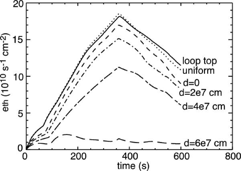
Figure 12: Temporal variation of $e_{th}$ in the simulations with various flare heating fucntion. Plotted are the loop top heating, the uniform heating and the footpoint heating with $d=0,2,4$ and $6\times 10^{7}$ cm, which are indicated in the figure.

Table 1: Parameters of the flares.

Parameter	2000 Nov 24	2000 Jul 14	2000 Nov 16
GOES class	X2.3	M3.7	C8.9
$H$ (erg s${}^{-1})$	2.7e28	6.4e27	1.9e27
$v_{foot}$ (cm s${}^{-1})$	1.2e6	1.2e6	6.7e5
$B_{foot}(G)$	449	117	106
$L_{x}$ (cm)	2.2e9	1.5e9	3.1e9
$L_{y}$ (cm)	3.5e9	4.2e9	5.2e9
$n_{0}$ (cm-3)	1.0e9	2.0e9	6.e8
$T_{0}$ (K)	1.0e7	8.0e6	8.e6
$B_{cr}$ (G)	41	44	11
$v_{in}$ (cm s${}^{-1})$	1.3e7	3.2e6	6.7e6
$v_{A}$ (cm s-1)	2.8e8	2.1e8	9.4e7
$M_{A}$	0.047	0.015	0.071
$R_{m}$	1.8e15	7.0e14	6.3e14
$E_{cs}$ (V m-1)	539	143	70
$\alpha$	0.6	0.55	0.65

Table 2: Magnetic flux $\phi$, ribbon length $L_{ribbons}$, magnetic field strength $B_{foot}$ and separation velocity $v_{foot}$ of the 2000 Nov. 24 flare. The effect of projection was corrected.

Parameter	east ribbon	west ribbon	average
$\phi$ (Mx)	1.0e21	7.6e20	8.8e20
$L_{ribbon}$ (cm)	3.1e9	5.8e9	4.5e9
$B_{foot}$ (G)	574	324	449
$v_{foot}$ (cm s-1)	1.4e6	1.0e6	1.2e6

Table 3: Magnetic flux $\phi$, ribbon length $L_{ribbons}$, magnetic field strength $B_{foot}$ and separation velocity $v_{foot}$ of the 2000 Jul. 14 flare. The effect of projection was corrected.

parameter	east ribbon	west ribbon	average
$\phi$ (Mx)	1.6e20	1.5e20	1.6e20
$L_{ribbon}$ (cm)	3.4e9	6.6e9	5.0e9
$B_{foot}$ (G)	144	91	117
$v_{foot}$ (cm s-1)	1.4e6	1.0e6	1.2e6

Table 4: Magnetic flux $\phi$, ribbon length $L_{ribbons}$, magnetic field strength $B_{foot}$ and separation velocity $v_{foot}$ of the 2000 Nov. 16 flare. The effect of projection was corrected.

Parameter	east ribbon	west ribbon	average
$\phi$ (Mx)	1.4e20	2.2e20	1.8e20
$L_{ribbon}$ (cm)	5.3e9	7.6e9	6.4e9
$B_{foot}$ (G)	143	69	106
$v_{foot}$ (cm s-1)	4.0e5	9.3e5	6.7e5

References

- Abbett & Hawley (1999) Abbett, W. P. & Hawley, S. L. 1999, ApJ, 521, 906
- Asai et al. (2004a) Asai, A., Yokoyama, T., Shimojo, M., & Shibata, K. 2004, ApJ, 605, L77
- Asai et al. (2004b) Asai, A., Yokoyama, T., Shimojo, M., Masuda, S., Kurokawa, H., & Shibata, K. 2004, ApJ, 611, 557
- Biskamp (1992) Biskamp, D. 1992, Nonlinear Magnetohydrodynamics, Cambridge: Cambridge Univ. Press
- Chen et al. (2004) Chen, P. F., Shibata, K., Brooks, D. H., & Isobe, H. 2004, ApJ, 602, L61
- Chen & Shibata (2000) Chen, P. F. & Shibata, K. 2000, ApJ, 545, 524
- Dere (1996) Dere, K. P. 1996, ApJ, 472, 864
- Domingo, Flech, & Poland (1995) Domingo, V., Fleck, B., & Poland, A. I. 1995, Sol. Phys., 162, 1
- Emslie et al. (2004) Emslie, A. G. et al. 2004, J. Geophys. Res., 199, A10104
- Erkaev, Semenov, & Jamitzky (2000) Erkaev, N. V., Semenov, V. S., & Jamitzky, F. 2000, Phys. Rev. Lett., 84, 1455
- Fletcher & Hudson (2001) Fletcher, L. & Hudson, H. 2001, Sol. Phys., 204, 71
- Fletcher, Pollock, & Potts (2003) Fletcher, L., Pollock, J. A., & Potts, H. 2003, Sol. Phys., 222, 279
- Forbes & Lin (2000) Forbes, T. G., & Lin, J. 2000, J. Atmos. Sol-Terr. Phys., 62, 1499
- Grigis & Benz (2005) Grigis, P. C. & Benz, A. O. 2005, ApJ, 625, L143
- Handy et al. (1999) Handy, B. N. et al. 1999, Sol. Phys., 187, 229
- Hara et al. (1992) Hara, H., Tsuneta, S., Lemen, J. R., Acton, L. W., & McTiernan, J. M., 1992, PASJ, 44, L135
- Hirsch (1988) Hirsch, C. 1988, Numerical Computation of Internal and External Flows, Vol. 1, New York: Wiley, 476
- Hori et al. (1997) Hori, K., Yokoyama, T., Kosugi, T., & Shibata, K. 1997, ApJ, 489, 426
- Innes, McKenzie, & Wang (2003) Innes, D. E., McKenzie, D. E., & Wang, T. 2003, Sol. Phys., 217, 247
- Isobe, Shibata, & Machida (2002) Isobe, H., Shibata, K., & Machida, S. 2002, Geophys. Res. Lett., 29(21), 2014
- Isobe et al. (2002) Isobe, H., Yokoyama, T., Shimojo, M., Morimoto, T., Kozu, H., Eto, S., Narugake, N., & Shibata, K. 2002, ApJ, 556, 528
- Isobe et al. (2003) Isobe, H., Shibata, K., Yokoyama, T., & Imanishi, K. 2003, PASJ, 55, 967
- Isobe et al. (2005) Isobe, H., Miyagoshi, T., Shibata, K., & Yokoyama, T. 2005, Nature, 434, 478
- Ji et al. (1998) Ji, H., Yamada, M., Hsu, S., & Kulsrud, R. 1998, Phys. Rev. Lett., 80, 3256
- Lin (2004) Lin, J. 2004, Sol. Phys., 222, 115
- Lin et al. (2005) Lin, J., Ko, Y.-K., Sui, L., Raymond, J. C., Stenborg, G. A., Jiang, Y., Zhao, S., & Mancuso, S. 2005, ApJ, 622, 1251
- Litvinenko, Forbes, & Priest (1996) Litvinenko, Y. E., Forbes, T. G., & Priest, E. R. 1996, Sol. Phys., 167, 445
- Martens (2003) Martens, P. C. H. 2003, Adv. Space Res., 32, 905
- Masuda et al. (1994) Masuda, S., Kosugi, T., Hara, H., Tsuneta, S., & Ogawara, Y. 1994, Nature, 371, 495
- McKenzie & Hudson (1999) McKenzie, D. E., & Hudson, H. S. 1999, ApJ, 519, L93
- Metcalf & Fisher (1996) Metcalf, T. R. & Fisher, G. H. 1996, ApJ, 462, 977
- Moon et al. (2003) Moon, Y.-J., Choe, G. S., Wang, H., Park, Y. D., & Cheng, C. Z. 2003, J. Korean Astron. Soc., 36, 61
- Narukage & Shibata (2005) Narukage, N. & Shibata, K. submitted to ApJ
- Nitta & Hudson (2001) Nitta, N. V. & Hudson, H. S. 2001, Geophys. Res. Lett., 28, 3801
- Nitta (2004) Nitta, S. 2004, ApJ, 610, 1117
- Noglik, Walsh, Ireland (2005) Noglick, J. B., Walsh, R. W., & Ireland, J. A&A in press.
- Ogawara et al. (1991) Ogawara, Y. Takano, T., Kato, T., Kosugi, T., Tsuneta, S., Watanabe, T., Kondo, I., & Uchida, U. 1991, Sol. Phys., 136, 1
- Ohyama & Shibata (1997) Ohyama, M. & Shibata, K. 1997, PASJ, 49, 249
- Ohyama & Shibata (1998) Ohyama, M. & Shibata, K. 1998, ApJ, 499, 934
- Parker (1957) Parker, E. N. 1957, J. Geophys. Res., 62, 509
- Petschek (1964) Petschek, H. E. 1964, in Physics of Solar Flares, AAS-NASA Symposium, ed. W. N. Hess (NASA SP-50), 425
- Priest (1982) Priest, E. R. 1982, Solar Magneto-Hydrodynamics, Dordrecht: Reidel
- Priest & Forbes (2000) Priest, E. R. & Forbes, T. G. 2000, Magnetic Reconnection MHD Theory and Applications, Cambridge: Cambridge Univ. Press
- Qiu et al. (2002) Qiu, J., Lee, J., Gary, D. E., & Wang, H. 2002, ApJ, 565, 1335
- Qin et al. (2004) Qiu, J., Wang, H., Cheng, C. Z., & Gary, D. E. 2004, ApJ, 604, 900
- Rubin and Burkstein (1967) Rubin, E. L. & Burkstein, S. Z. 1967, J. Comput. Phys. 2, 17
- Saba, Gaeng, & Tarbell (2002) Saba, J. L. R., Gaeng, T., Tarbell, T. D. 2002, in Multi-Wavelength Observations of Coronal Structures and Dynamics – Yohkoh 10th Anniversary Meeting, ed. P. C. H. Martens and D. P. Cauffman, 175
- Scherrer (1995) Scherrer, P. H. et al. 1995, Sol. Phys., 162, 129
- Scholer (1989) Scholer, M. 1989, J. Geophys. Res., 94, 8805
- Shibata (1999) Shibata, K. 1999, Ap&SS, 264, 129
- Shibata et al. (1995) Shibata, K. Masuda, S. Shimojo, M. Hara, H. Yokoyama, T. Tsuneta, S. Kosugi, T. & Ogawara, Y. 1995, ApJ, 451, L83
- Shimojo et al. (2001) Shimojo, M., Shibata, K., Yokoyama, T., & Hori, K. 2001 ApJ, 550, 1051
- Shiota et al. (2003) Shiota, D., Yamamoto, T. T., Sakajiri, T., Isobe, H., Chen, P. F., & Shibata, K. 2003, PASJ, 55, L35
- Spitzer (1956) Spitzer, L. 1956, Physics of Fully Ionized Gases, New York: Interscienc
- Sweet (1958) Sweet, P. A. 1958, in IAU Symp. 6, Electromagnetic Phenomena in Cosmical Physics, ed. B. Lehnert, Camgridge:Cambridge Univ. Press, 123
- Tajima & Shibata (1997) Tajima, T. & Shibata, K. 1997, Plasma Astrophysics, Reading, MA: Addison- Wesley
- Takasaki et al. (2004) Takasaki, H., Asai, A., Kiyohara, J., Shimojo, M., Terasawa, T. Takei, Y., & Shibata, K. 2004, ApJ, 613, 592
- Tanuma et al. (2001) Tanuma, S., Yokoyama, T., Kudoh, T., & Shibata, K. 2001, ApJ, 551, 312
- Tsuneta (1996) Tsuneta, S., 1996, ApJ, 456, 840
- Tsuneta et al. (1991) Tsuneta, S., et al. 1991, Sol. Phys., 136, 37
- Tsuneta et al. (1992) Tsuneta, S., Hara, H., Shimizu, T., Acton, L. W., Strong, K. T., Hudson, H. S., & Ogawara, Y. 1992, PASJ, 44, L63
- Ugai (1986) Ugai, M. 1986, Phys. Fluids,29, 3659
- Wang et al. (2003) Wang, H., Qui, J., Jing, J., & Zhang, H. 2003, ApJ, 593, 564
- Yokoyama et al. (1994) Yokoyama, T. & Shibata, K. 1994, ApJ, 436, L197
- Yokoyama et al. (2001) Yokoyama, T., Akita, K., Morimoto, T., Inoue, K., & Newmark, J. ApJ, 546, L69
- Zhang, Solanki, & Wang (2003) Zhang, J., Solanki, S. K., & Wang, J. 2003, A&A, 399, 755
- Zhang & Wang (2002) Zhang, J. & Wang, J. 2002, ApJ, 566, L117