, ,
A closer look at the spectrum and small scale anisotropies of UHECRs
Abstract
We present results of numerical simulations of the propagation of ultra high energy cosmic rays (UHECRs) over cosmological distances, aimed at quantifying the statistical significance of the highest energy data on the spectrum and small scale anisotropies as detected by the AGASA experiment. We assess the significance of the lack of a GZK feature and its compatibility with the reported small scale anisotropies.
Assuming that UHECRs are protons from extragalactic sources, we find that the small scale anisotropies are incompatible with the reported spectrum at a probability level of . Our analysis of the AGASA results shows the power of combining spectrum and small scale anisotropy data in future high statistics experiments, such as Auger.
1 Introduction
The problem of the origin of ultra-high energy cosmic rays (UHECRs) is a collection of several questions that will only be solved by high statistics observations around eV. The first question is whether there is a Greisen-Zatsepin-Kuzmin [1] (GZK) feature in the spectrum of UHECRs due to photopion interactions with the cosmic microwave background (CMB). Photopion production is expected to generate a flux suppression around eV possibly followed by a recovery. The statistical significance achieved by current experiments is not sufficient to clarify whether the feature is present and what is its exact shape (see, e.g., [2]), but future data from the Pierre Auger Observatory [3] should resolve this issue. The second part of the problem is related to the identification of a class or several classes of sources that can accelerate particles to energies in excess of eV. The search for sources of UHECRs will likely be a long process requiring the identification of anisotropies in the arrival direction of the highest energy cosmic rays as well as multiparticle observations of high energy sources (see, e.g., [4, 5]). Large scale anisotropies may indicate the generic host of sources while small scale anisotropies can eventually identify single sources directly. As small scale anisotropies start to become apparent with small number of events per source (e.g., doublets and triples), an estimate of the number density of the sources becomes feasible (see, e.g. [6, 7]). For a clear source identification with single source spectral measuments, a future generation of experiments will be necessary.
If astrophysical sources are responsible for the acceleration of UHECRs, the mean density of sources can be determined by analyzing small scale anisotropies (SSA) in the arrival directions that should become apparent as large data sets of the highest energy events become available. So far the only experiment to report SSA is AGASA [8] and estimates for the number density of sources range from to with a large uncertainty [6] (see [7] for other estimates). In Ref. [6], a full numerical simulation of the propagation was performed accounting for the statistical errors in the energy determination and the AGASA acceptance with the conclusion that the AGASA small scale anisotropies is consistent with a density of sources . This source density corresponds to a luminosity per source of at energies eV and a best fit injection spectrum in the form of a power law has a spectral index if the source luminosity has no significant evolution with redshift. For the case of strong source evolution, in [6] it was assumed that the luminosity varies as a function of redshift as and the best fit slope at injection is . These fits are dominated by the energy regions with the largest number of events, i.e., at eV, such that a dominant contribution from galactic sources at these energies may significantly affect these results. The issue of the energy region where the transition from a galactic to extragalactic origin takes place is currently a subject of much debate. While the traditional view is that the ankle is indeed determined by such a transition, some recent work [9, 10] have proposed an alternative picture, in which the ankle is the natural result of the pair production process on cosmological propagation of extragalactic protons. The key issue in this class of models is the chemical composition, since a transition from heavy to light elements is predicted [9, 10]. A small contamination of the extragalactic component with iron nuclei would destroy the pair production dip and invalidate this model [10, 15]. If the ankle is due to this mechanism, the data at energies above and around the ankle are well fit by an injection spectrum in the form of a power law with slope and a low energy cutoff that can be the result of the appearance of a magnetic horizon [11, 12, 14].
The results on small scale anisotropies, obtained for cosmic rays at energies above eV, are not significantly affected by a possible galactic contamination at lower energies. Moreover at such high energies the effect of the galactic magnetic field is expected to not affect the propagation in a significant way.
The role of the intergalactic magnetic field is less constrained as different simulations give different estimates for the magnitude and spatial structure of these fields (see, e.g., [16, 17]). A homogeneous magnetic field spread through the whole universe would leave the spectrum of diffuse cosmic rays unchanged with respect to the case of the absence of magnetic field [13]. Here, we assume that intergalactic magnetic fields can be neglected for particles with energies above eV. This assumption holds if magnetic fields in the intergalactic medium are less than if the reversal scale is Mpc and the small scale anisotropies are evaluated on angles of degrees [6]. This magnitude field is compatible with observational bounds [18] and detailed numerical simulations in [16] (however, see [17] for different results). These magnetic field calculations are the result of the formation of the large scale structure of the universe. Other authors considered alternative possibilities, for instance, related to the early stages of evolution of galaxies [19], but in most cases the results are very model dependent and are affected by further evolution of magnetic fields during large scale structure formation. It is likely that UHECR observations will eventually allow us to measure the strength of the intergalactic magnetic field and get information about its structure (see, e.g., [14, 20]).
In the present paper, we address the significance of a detection of the GZK feature together with the identification of small scale anisotropies. We combine these two types of observations by AGASA in order to check their compatibility. In §2, we briefly describe the Monte Carlo code used to determine the spectra and the SSA. In §3, we discuss simulated spectra of AGASA and HiRes with regards to the presence or absence of a GZK feature. In §4, we calculate the two-point correlation function for different choices of the angular binning and combine the spectrum and SSA studies. We conclude in §5.
2 The Monte-Carlo code
The propagation of UHECRs is simulated using a Monte-Carlo code described in [2, 6]. We assume that UHECRs are protons injected with a power-law spectrum by extragalactic sources. The injection spectrum in taken to be of the form:
| (1) |
where is the spectral index and is the maximum injection energy at the source. We fix and since these values reproduce well the experimental results in the lower energy, high statistics region eV to eV [2]. Here, we focus on events above , which are generated at , therefore, source evolution is only marginally relevant [6]. We simulate the propagation of protons from the source to the observer by including the photo-pion production, pair production, and adiabatic energy losses due to the expansion of the universe. The photo-pion production is treated as a discrete energy loss process and is simulated using the event generator SOPHIA [21].
We use a constrained simulation where particles are propagated until the number of detected events above some energy threshold reproduces the experimental results. By normalizing the simulated flux by the number of events above a given energy, where experiments have high statistics, we can estimate the fluctuations in the number of events above a higher energy where experimental results are sparse. In this way, we have a direct handle on the fluctuations that can be expected in the observed flux due to the stochastic nature of the photo-pion production and to cosmic variance.
In choosing the initial particles to be propagated, we employ two different physical scenarios: a) a continuous distribution of sources; and b) a discrete distribution of point sources with a given density. For the continuous distribution a source distance is generated at random from a uniform distribution in a universe with and . In an Euclidean universe, every spherical shell contributes equally to the generated flux of particles. The flux from a source scales as , where is the distance between the source and the observer, while the number of sources between and scale as , so that the probability that a given event has been generated by a source at distance is independent from . In a flat universe with a cosmological constant this is still true provided the distance is taken to be
| (2) |
where is the age of the universe when the event was generated, is the present age of the universe, and is the scale factor of the universe. Once a particle has been generated, the code propagates it to the detector calculating energy losses and taking into account the energy and angular resolution of the detector.
For a discrete distribution of point sources, we first generate the positions of sources with a given spatial density and then emit particles choosing randomly from the source positions. The source redshifts are generated with a probability distribution proportional to
| (3) |
where is the defined in Eq. (2) and gives the relation between time and redshift for a flat universe with a cosmological constant (see, e.g., the expression given in [22]). The source positions on the celestial sphere are chosen uniformly in right ascension and with a declination distribution proportional to .111The declination is defined as being on the equatorial plane and at the poles, so .
Since we neglect the effects of the magnetic fields on the propagation, we ignore sources outside the experimental field of view and assign to visible sources a probability proportional to:
| (4) |
where takes into account the distance dependence of the solid angle and is the relative exposure of the experiment in the given direction. The positions for particle injection are chosen randomly from the assigned source positions and propagation proceeds as in the previous case.
The last point worth stressing is the importance of the statistical errors in the energy determination. The statistical errors in the energy are accounted for in our simulation by assigning a detection energy chosen at random from a gaussian distribution centered at the arrival energy and with width . As we show in the next section and in [2], the presence of a statistical error in the energy determination does affect the shape of the spectrum of UHECRs close to the GZK feature. This point was also made recently in [23] for the case of Log-normal errors in the energy determination.
3 Simulated spectra of AGASA and HiRes
There are several reasons to simulate the expected spectrum of UHECRs, rather than an analytical treatment, including the ability to introduce detector-related features which can affect the results. For instance, the energy dependence and zenith angle dependence of the acceptance of the experiment can be included as well as statistical and systematic errors associated with the energy detemination of each event. In order to illustrate the importance of this point, we calculated the spectrum of UHECRs from a uniform distribution of sources with and without statistical errors. In Fig. 1, we plot the expected fluxes (small square inside the main plot) with (solid line) and without (dashed line) 30% statistical error in the energy determination. The main plot illustrates the flux multiplied by the third power of the energy without statistical error (dashed line), and with a 30% statistical error in the energy determination (solid line).
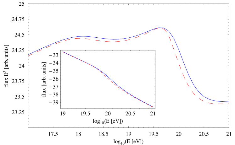
From Fig. 1, it is clear that the effect of the statistical error on the flux multiplied by is to smear the shape of the GZK feature and to move its position toward higher energies. This effect is due to the steeply falling spectrum and to its slope changes, so that the probability of misplacing an event from a lower to a higher energy bin is larger than in the opposite direction.
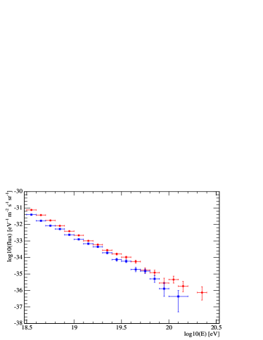
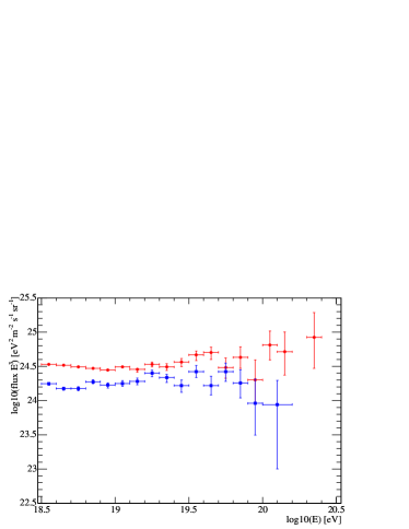
Results from the two largest exposure experiments, AGASA and HiRes, are claimed to be inconsistent. The fluxes from AGASA and HiResI are plotted in the left panel of Fig. 2, while the fluxes multiplied by are in the right panel. The flux figure suggests that despite the different techniques used by the two experiments, they appear to be in rather good agreement. There seems to be a systematic shift and some discrepancy at the highest energy bins. Their discrepancies are made more evident in the right panel, due to the amplification factor. At energies eV, the HiRes spectrum shows a hint of a cutoff, while the AGASA spectrum continues unabated. In Ref. [2] we showed that a systematic overestimate of the AGASA energies by 15% and an underestimate of the HiRes energies by the same amount would in fact bring the two data sets in much better agreement in the region of energies below . At higher energies, the very low statistics of both experiments hinders any statistically significant claim for either detection or the lack of the GZK feature.
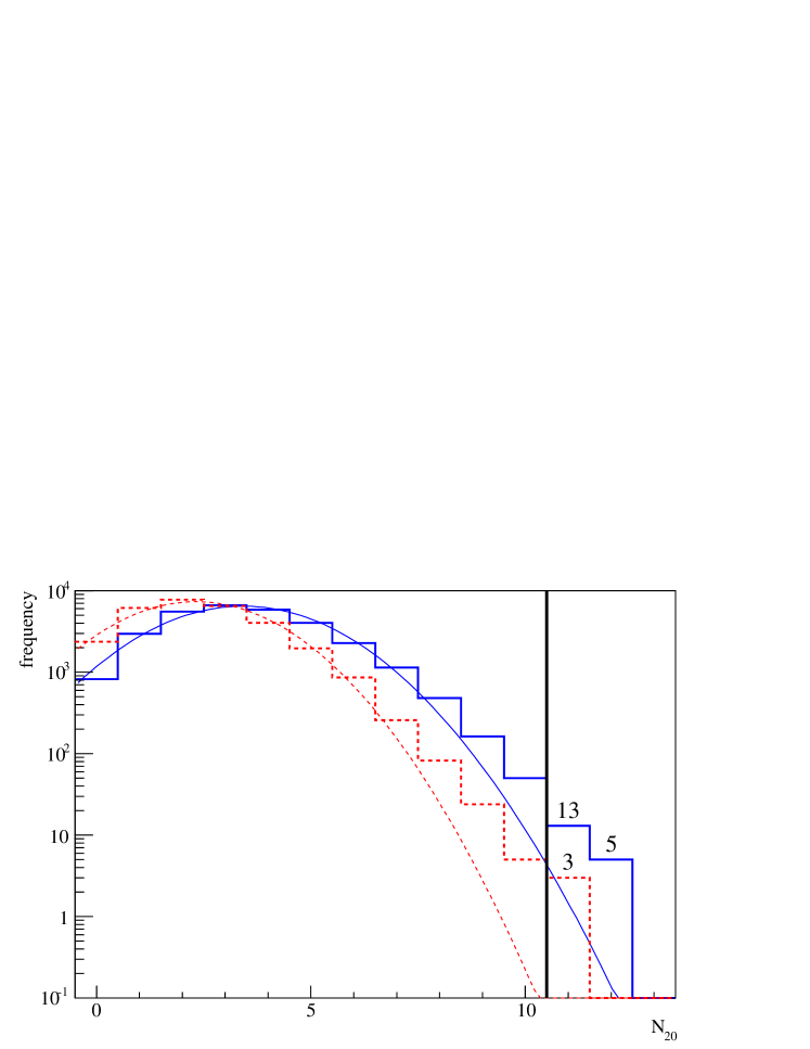
To clarify the dangers of low statistics, we simulated the AGASA spectrum normalizing at (instead of as in Ref. [2]) without the statistical error on the energy determination and with a 30% error. We generated 30000 realizations of spectra with 72 events above like the AGASA data and recorded the number of events with energies above in each realization. When the experimental error is taken into account, we obtained events above . In the case of no errors, the number is .
Assuming a gaussian distribution with the above numbers, we would incorrectly conclude that the 11 AGASA events above are a discrepancy, corresponding to a probability of . In Fig. 3, we plot the histogram of the number of events above in each realization. The dashed histogram is the result of the simulation without statistical errors, whereas the solid one is the result of adopting a 30% statistical error. The thin lines are gaussian fits to the histograms. As it is clear from Fig. 3, the distributions are not gaussian such that the naive estimates above of the discrepancy and of the probability are incorrect. Of the 30000 realizations we simulated the number of spectra presenting 11 or more events with energy above is 18 for the simulations with statistical errors. This corresponds to a probability of that in terms of gaussian errors would correspond to a discrepancy of about . A similar calculation was performed for the degenerate injection spectrum with and redshift evolution of the luminosity . In this case the probability becomes ,basically identical to the previous case.
In [2], we also considered the effect of a possible systematic error in both the AGASA and HiRes experiments. To match the two spectra, we assumed that the AGASA energies had been overestimated by 15% and that the HiRes energies were underestimated by the same amount. In this case, the number of events above in the rescaled AGASA data set is between 6 and 7, while the number of events above is about 47. We simulated 30000 realizations of this statistics above and counted the number of events in each realization with energies above . In this case, the number of realizations with 7 or more events above turned out to be 179, which corresponds to a probability of or a discrepancy of in terms of gaussian errors. Since there are several events with energy very close to we also considered the case of a number of events above equal to 6. Counting the simulated realizations with 6 or more events above , we obtained a probability of 0.024 or about .
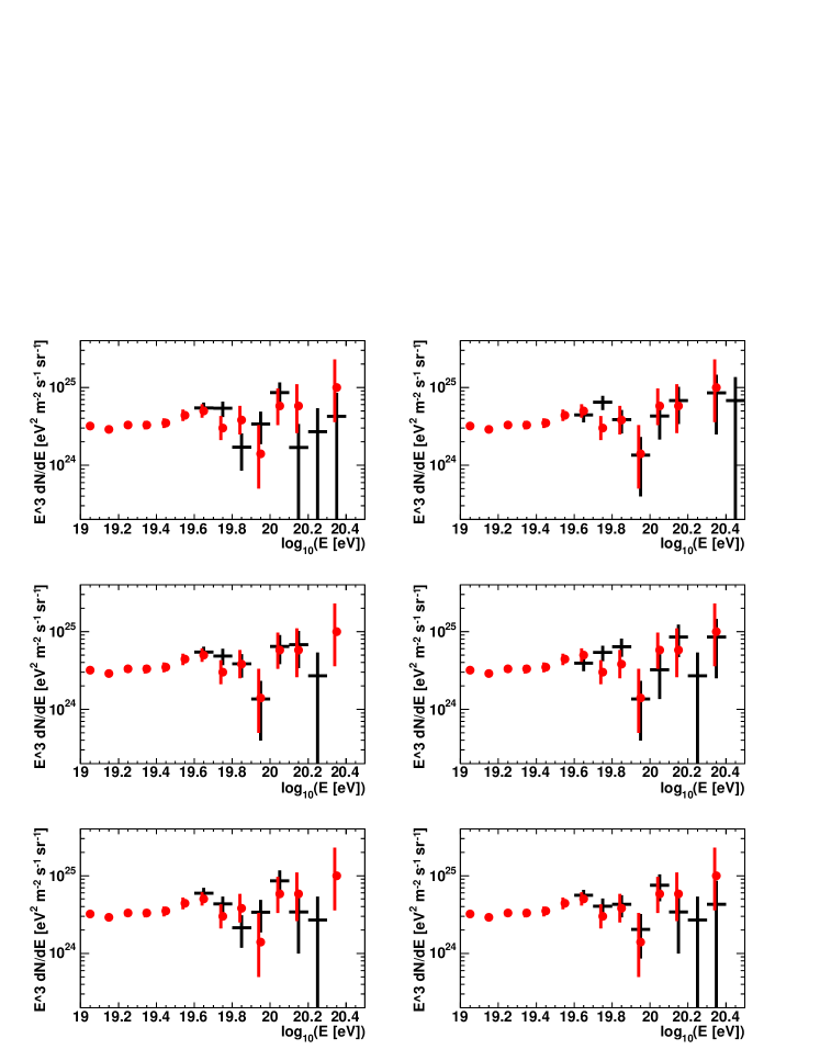
These statistical considerations are the result of averages over large samples of realizations of source distributions, therefore one might wonder whether the spectra of UHECRs for those realizations that have a large number of events at ultra high energies are characterized by a pronounced GZK feature or are similar to the AGASA spectrum. To resolve this issue we plot, in Fig. 4, the spectra of some of the realizations that showed 11 or more events above . These spectra closely resemble the AGASA spectrum: all of them show no evidence of a GZK suppression, despite the fact that in the lower energy region they all fit the data quite well. This shows that an AGASA-like spectrum is not that improbable, even if the average cosmic ray spectrum can be expected to show a GZK feature.
It is worth noticing that a few of the AGASA events are just a few percent above , so that any small error in the energy assignment to one or more events would affect the statistical analyses discussed above. For instance, if just one of the events above had a real energy below , the probability of reproducing the AGASA result would become (). On the other hand, if one of the events below had actually an energy above then the probability would become (). So, changing the number of detected events above by just one unit changes the probabilities of reproducing the AGASA results by relatively large amounts. These results again indicate the excessively low statitics of events, and conclusions concerning the spectrum of UHECRs at these energies should not be considered as reliable.
This argument applies as well to the case of the HiRes experiment. Although HiRes data appears to be consistent with the presence of the GZK feature, such a conclusion is also premature. To show this, we assumed that the actual flux of UHECRs is consistent with the spectrum measured by AGASA (which is usually considered to be inconsistent with the GZK feature) and selected events from such spectrum. Then each event is either accepted or rejected according to the HiRes aperture [25] (the aperture of HiRes increases with energy while that of AGASA is constant at high energies). This procedure is repeated until the number of accepted events with energy above corresponds to the one measured by HiRes (namely 27). We then count the number of events with energies above in each realization and calculate the probability of having one or less events (namely the HiRes number of detections) in that energy region. We find that such probability is , corresponding to about in terms of gaussian errors. We also tried to vary the parameters related to the injection spectrum without appreciable changes in the final probabilities. Summarizing, HiRes is not unlikely to be observing events extracted at random from the AGASA spectrum. In other words, both AGASA and HiRes simply do not have the necessary statistics of events required to assess either the presence or absence of the GZK feature in the spectrum of UHECRs.
4 Combining spectrum and small scale anisotropies
If UHECRs are accelerated in astrophysical sources, then small scale anisotropies (SSA) should be observed at the highest energies. The level of SSA depends on the average density of sources and on the strength of possible magnetic fields in the intergalactic medium. Simulations of the formation of the large scale structure of the universe find that most of the volume of the universe is very weakly magnetized, and the typical deflections at energies above eV are smaller than experimental accuracy [16] (however, see [17] for a different conclusion). UHECR Astronomy should become possible at the highest energies starting with the detection of either small or large scale anisotropies. Observations of SSA can be used to infer the average density of sources and the typical luminosity of each source, an information which is not accessible through the spectrum of diffuse UHECRs alone.
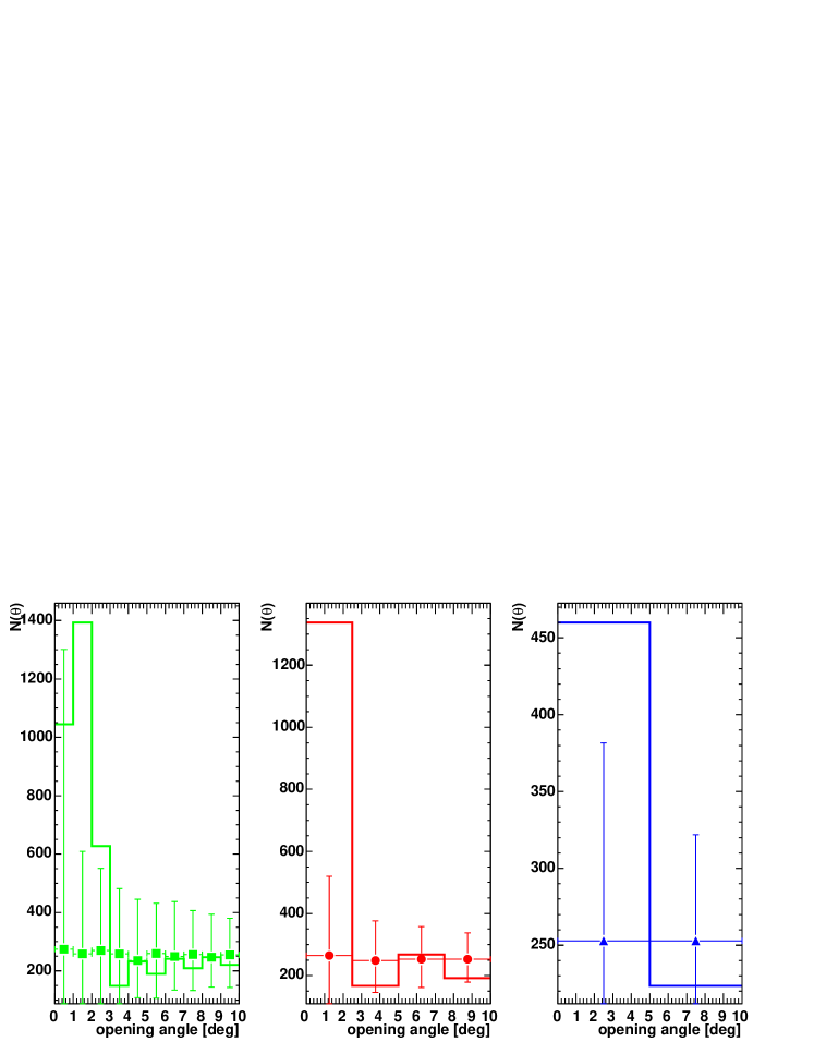
AGASA has reported the detection of SSA [8], whose significance has been questioned in [27, 28]. Even if not significant, the SSA data from AGASA can be used to exemplify the power of combining SSA and the spectrum. In [6], the best fit density of sources based on AGASA SSA was estimated to be , although with large uncertainties (see also [7]). In Fig. 5, we plot the two point correlation function, defined as in [6] for different choices of the angular binning over which the multiplets are searched for (1 degree in the left panel, 2.5 degrees in the central panel, and 5 degrees in the right panel). The points with error bars are the expected (simulated) two point correlation function on the given angular scale for a homogeneous distribution of sources. It is clear that the statistical significance of the small scale anisotropies decreses significantly for angular binning on scales smaller or larger than degrees.
In Section 3, we concluded that the measurements of the spectrum by AGASA and HiRes collaborations are not yet statistically significant around the GZK feature. In those calculations, we used the assumption of a uniform distribution of diffuse sources. We repeat these calculation for a discrete distribution of sources with density . With this source distribution, the average separation between sources is of the order of Mpc, such that the shape of the GZK feature should be more pronounced than for the uniform case. As a consequence, the disagreement of AGASA with the prediction of a GZK suppression should become more pronounced. In order to demonstrate this point, we simulate 50000 realizations of the AGASA statistics above , in a scenario of discrete sources with density . In this case, we find 6 realizations out of the 50000 producing 11 or more events above and this corresponds to a probability of about or . Clearly, the result is less (more) severe for source densities ().
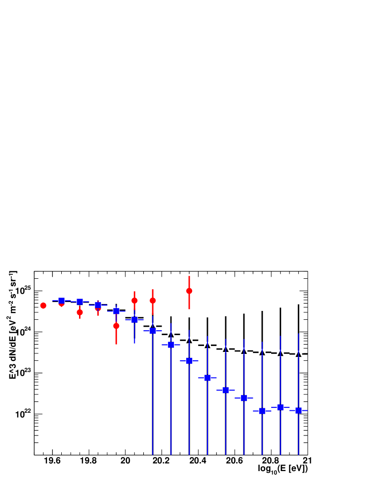
This result is further illustrated in Fig. 6 where we show a comparison between the spectra obtained for the AGASA statistics of events for a homogeneous distribution of sources (black triangles with error bars) and point sources with density (blue squares with error bars). The circles are the AGASA data.
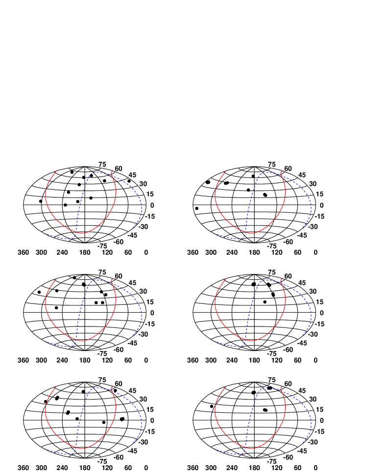
In conclusion, the spectrum of AGASA is inconsistent (at the level) with a GZK feature generated by the source distribution implied by the reported SSA. These discrepancies could be more severe if the maximum energy at the accelerators is lower than that assumed above. In addition, the distribution in the sky of the 11 (or more) events in these realizations are not necessarily similar to the AGASA case. We show our simulated sets of events in Fig. 7. With the exception of the first map in the top left corner, all the realizations appear to have a higher number of multiplets when compared with AGASA observations. In other words, if UHECR sources are astrophysical proton accelerators, there is an inconsistency between the spectrum and small scale anisotropies of the AGASA experiment. If we require that both the spectrum and the sky distributions are correctly reproduced with a source density , the probability that this occurs in the AGASA data is . This exercise shows that the combination of the spetral and anisotropy information is a powerful tool to estimate the density of sources of UHECRs and identify possible internal inconsistencies in the data. As the wealth of data expected from Auger becomes available in the next few years, this type of study should help the identification of UHECR sources.
5 Conclusions
We investigated numerically the propagation of UHECRs using a Monte Carlo code originally developed in [2] and generalized to include astrophysical point sources in [6]. The code contains all the main particle physics aspects of the propagation, as well as several detector-related features (exposures, angle and energy dependent acceptances, statistical error in the energy determination, and limited statistics of events). We performed simulations constrained by the number of observed events above eV and compared the number of events above eV observed by AGASA and HiRes. For AGASA we jointly analyzed the observed spectrum and small scale anisotropies. The combination of the two types of information strengthens the constraints on the presence of a the GZK feature or of clustering of events on small angular scales.
In conclusion, we first presented the results of our simulations of the AGASA and HiRes statistics of events similar to the analysis in [2]. We followed an alternative route and reached very similar conclusions. We simulated 30000 realizations with different scenarios and showed that the probability distribution of these events is non-gaussian. When expressed in terms of gaussian standard deviations the probability to record 11 or more events with energies above eV corresponds to . If a systematic energy decrease of 15% is introduced, the probability of a AGASA spectrum becomes . We also found that the probability of finding a spectrum similar to HiRes (one or less than one event at energies above eV) is 3%. The two spectra cannot therefore be considered inconsistent with each other at a level better than .
We also analyzed the small scale anisotropies as detected by AGASA to stress the fact (already found in [27]) that the statistical significance of the clustering depends on the angular scale with which the data are binned. We clarified this issue by calculating the two point correlation function for the AGASA data and for the simulated data as obtained from a homogeneous distribution of sources. It is clear from this result that the angular binning chosen by AGASA is the one that optimizes the small angle clustering signal, but the statistial significance of such signal decreases for smaller or larger angular binnings.
Finally, we combined the spectrum and the small scale clustering information. Choosing a source density of obtained by fitting the number of doublets and triplets of AGASA (assumed to be real), we recalculate the spectrum of UHECRs. As expected, for this source density the GZK feature is more pronounced than that obtained for a homogeneous distribution of sources and the discrepancy with respect to the AGASA spectrum is at the level of . Moreover, by simulating 50000 realizations of the propagation, we obtained the arrival directions of the events in those realizations that show a number of events above eV equal to or larger than that of AGASA (11 events). Only 6 out the 50000 realizations fulfill the spectrum requirement and of the 6 realizations only one has a sky distribution of the events with resembles the AGASA one (no multiplets). We conclude that, if the sources of UHECRs are astrophysical proton accelerators, the reported small scale anisotropies are not compatible with the spectrum detected by the AGASA experiment at the level of probability. In other words only 1 realization out of 50000 has a spectrum and a sky distribution of the events that are compatible with the AGASA data.
References
References
- [1] Greisen K 1966 Phys. Rev. Lett.16 748 Zatsepin G T and Kuzmin V A 1966 Sov. Phys. JETP Lett. 4 78
- [2] De Marco D, Blasi P and Olinto A V 2003 Astropart. Phys. 20 53
- [3] Cronin J W 2001 Pierre Auger Observatory, Proceedings of ICRC 2001
- [4] Ferrigno C, Blasi P and De Marco D 2005 Astropart. Phys. 23 211
- [5] Gabici S and Aharonian F 2005 Preprint astro-ph/0505462
- [6] Blasi P and De Marco D 2004 Astropart. Phys. 20 559
- [7] Isola C and Sigl G 2002 Phys. Rev.D66 3002 Yoshiguchi H, Nagataki S, Tsubaki S and Sato K 2003 Astrophys. J. 586 1211 Yoshiguchi H, Nagataki S and Sato K 2003 Astrophys. J. 592 311 Takami H, Yoshiguchi H, Sato K 2005 Preprint astro-ph/0506203 Dubovsky S L, Tinyakov P G and Tkachev I I 2000 Phys. Rev. Lett.85 1154 Fodor Z and Katz S D 2001 Phys. Rev.D63 023002
- [8] Takeda M et al1999 Astrophys. J. 522 225 Uchihori Y et al2000 Astropart. Phys. 13 151 Hayashida N et al2000 Preprint astro-ph/0008102
- [9] Berezinsky V S, Gazizov A and Grigorieva S 2002 Preprint hep-ph/0204357 Berezinsky V S, Gazizov A and Grigorieva S 2003 Preprint astro-ph/0302483
- [10] Berezinsky V S, Gazizov A and Grigorieva S 2005 Phys. Rev. Lett.612 147
- [11] Stanev T, Engel R, Mucke A, Protheroe R J and Rachen J P 2000 Phys. Rev.D62 093005
- [12] Aloisio R and Berezinsky V S 2005 Astrophys. J. 625 249
- [13] Aloisio R and Berezinsky V S 2004 Astrophys. J. 612 900
- [14] Lemoine M 2005 Phys. Rev.D71 083007
- [15] Allard D, Parizot E, Khan E, Goriely S and Olinto A V 2005 Preprint astro-ph/0505566
- [16] Dolag K, Grasso D, Springel V and Tkachev I 2005 J. Cosmol. Astropart. Phys. JCAP01(2005)009 Dolag K, Grasso D, Springel V and Tkachev I 2004 JETP Lett. 79 583 Dolag K, Grasso D, Springel V and Tkachev I 2004 Pisma Zh. Eksp. Teor. Fiz. 79 719
- [17] Sigl G, Miniati F and Ensslin T 2004 Phys. Rev.D70 043007 Sigl G, Miniati F and Ensslin T 2003 Phys. Rev.D68 043002
- [18] Blasi P, Burles S, Olinto A V 1999 Astrophys. J. Lett. 514 L79
- [19] Kronberg P P, Lesch H and Hopp U 1999 Astrophys. J. 511 56
- [20] Deligny O, Letessier-Selvon A and Parizot E 2004 Astropart. Phys. 21 609
- [21] Mucke A, Engel R, Rachen J P, Protheroe R J and Stanev T 2000 Comput. Phys. Commun. 124 290
- [22] Berezinsky V and Grigorieva S 1988 Astron. Astroph. 199 1
- [23] Albuquerque I F M, Smoot G F 2005 Preprint astro-ph/0504088
- [24] Abu-Zayyad T et al[High Resolution Fly’s Eye Collaboration] 2005 Astropart. Phys. 23 157
- [25] Abbasi R U et al[High Resolution Fly’s Eye Collaboration] 2004 Phys. Rev. Lett.92 151101
- [26] Takeda M et al2003 Astropart. Phys. 19 447
- [27] Finley C B and Westerhoff S 2004 Astropart. Phys. 21 359
- [28] Cronin J W 2005 Nuclear Physics B (Proc. Suppl.) 138 465