Neptune’s Migration into a Stirred–Up Kuiper Belt:
A Detailed Comparison of Simulations to Observations

Abstract

Nbody simulations are used to examine the consequences of Neptune’s outward migration into the Kuiper Belt, with the simulated endstates being compared rigorously and quantitatively to the observations. These simulations confirm the findings of Chiang et al. (2003), who showed that Neptune’s migration into a previously stirred–up Kuiper Belt can account for the Kuiper Belt Objects (KBOs) known to librate at Neptune’s 5:2 resonance. We also find that capture is possible at many other weak, high–order mean motion resonances, such as the 11:6, 13:7, 13:6, 9:4, 7:3, 12:5, 8:3, 3:1, 7:2, and the 4:1. The more distant of these resonances, such as the 9:4, 7:3, 5:2, and the 3:1, can also capture particles in stable, eccentric orbits beyond 50 AU, in the region of phase space conventionally known as the Scattered Disk. Indeed, $90\%$ of the simulated particles that persist over the age of the Solar System in the so–called Scattered Disk zone never had a close encounter with Neptune, but instead were promoted into these eccentric orbits by Neptune’s resonances during the migration epoch. This indicates that the observed Scattered Disk might not be so scattered. This model also produced only a handful of Centaurs, all of which originated at Neptune’s mean motion resonances in the Kuiper Belt. However a noteworthy deficiency of the migration model considered here is that it does not account for the observed abundance of Main Belt KBOs having inclinations higher than $15^{\circ}$.

In order to rigorously compare the model endstate with the observed Kuiper Belt in a manner that accounts for telescopic selection effects, Monte Carlo methods are used to assign sizes and magnitudes to the simulated particles that survive over the age of the Solar System. If the model considered here is indeed representative of the outer Solar System’s early history, then the following conclusions are obtained: (i.) the observed 3:2 and 2:1 resonant populations are both depleted by a factor of $\sim 20$ relative to model expectations; this depletion is likely due to unmodeled effects, possibly perturbations by other large planetesimals, (ii.) the size distribution of those KBOs inhabiting the 3:2 resonance is significantly shallower than the Main Belt’s size distribution, (iii.) the total number of KBOs having radii $R>50$ km and orbiting interior to Neptune’s 2:1 resonance is $N\sim 1.7\times 10^{5}$; these bodies have a total mass of $M\sim 0.08(\rho/\mbox{1 gm/cm${}^{3}$})(p/0.04)^{-3/2}$ M_⊕ assuming they have a material density $\rho$ and an albedo $p$. We also report estimates of the abundances and masses of the Belt’s various subpopulations (e.g., the resonant KBOs, the Main Belt, and the so–called Scattered Disk), and also provide upper limits on the abundance of Centaurs and Neptune’s Trojans, as well as upper limits on the sizes and abundances of hypothetical KBOs that might inhabit the $a>50$ AU zone.

1 Introduction

The Kuiper Belt is the vast swarm of small bodies that inhabit the outer Solar System beyond the orbit of Neptune. These Kuiper Belt Objects (KBOs) that inhabit this Belt are relics of the solar system’s primordial planetesimal disk—they are bits of debris that failed to coalesce into other large planets. The Kuiper Belt is also of great interest since it preserves a record of the outer Solar System’s early dynamical history. This is reflected in the KBOs’ curious distribution of orbits, which suggest that there was considerable readjustment of the Solar System’s early architecture. The possibility that the orbits of the giant planets may have shifted significantly (that is, after the solar nebula gas had already dissipated) was first demonstrated by the accretion simulations of Fernandez & Ip (1984); they showed that as the growing giant planets gravitationally scatter the residual planetesimal debris, they can exchange angular momentum with the debris disk in a way that causes the planets’ orbits to drift. Malhotra (1993b) later showed that an episode of outwards migration by Neptune by at least $\Delta a\simeq 5$ AU could also account for Pluto’s peculiar orbit, which resides at Neptune’s 3:2 resonance with an eccentricity of $e\simeq 0.25$. In this scenario, Pluto’s large eccentricity is a consequence of it having been captured by Neptune’s advancing 3:2 resonance, which pumped Pluto’s $e$ up as it shepherded the small planet outwards. Further support for this planet–migration scenario is provided by the subsequent discovery of numerous other KBOs also inhabiting Neptune’s 3:2 resonance with eccentricities similar to model predictions (Malhotra, 1995), as well as by more modern Nbody simulations of the orbital evolution of giant planets while they are still embedded in a massive planetesimal disk (Hahn & Malhotra 1999; Gomes et al. 2004).

The purpose of the present work is to use higher–resolution simulations to update this conventional model of Neptune’s migration into the Kuiper Belt. This model’s strengths, as well as its weaknesses, will be assessed quantitatively by rigorously comparing the simulations’ endstates to current observations of the Belt. In the following, we execute two simulations that track the orbital evolution of the four migrating giant planets plus $10^{4}$ massless test particles (the latter representing the KBOs) over the age of the Solar system. In one simulation the initial state of the Kuiper Belt is dynamically cold (i.e., the particles have initial eccentricities and inclinations of $e$ and $\sin i\sim 0.001$), while the second simulation is of a Kuiper Belt that is initially stirred–up a modest amount (i.e., $e$ and $\sin i\sim 0.1$). We then use a Monte Carlo method to assign sizes (and hence magnitudes) to the simulated KBOs; this allows us to account for the telescopic biases that tends to select those KBOs that inhabit orbits that are more favorable for discovery over those KBOs in less favorable orbits. Then, by comparing the resulting model Kuiper Belts with the current observational data, we rigorously test the planet–migration scenario as well as obtain a more realistic assessment of the abundance of KBOs. This analysis will also provide the relative abundance of the Belt’s various subpopulations—the resonant KBOs, the Main Belt Objects, the Scattered Disk, plus the Centaurs and Neptune’s Trojans.

The paper is organized as follows. Section 2 describes the so–called ‘standard model’ that is considered here, as well as the numerical methods to be employed. Results from two simulations of the Kuiper Belt are reported in Sections 3 and 4, while Section 5 examines the Kuiper Belt inclination problem. Section 6 details the Monte Carlo model that is then used in Sections 7–10 to assess the relative abundance of the Belt’s various subpopulations, with a final tally of the Belt’s total population given in Section 11. Section 12 comments on some important unmodeled effects, and Section 13 summarizes the results.

2 Simulating planet migration

The MERCURY6 Nbody integrator (Chambers, 1999) is used to track the orbital evolution of the four giant planets plus numerous massless particles. In our simulations, planet migration is implemented by applying an external torque to each planet’s orbit so that its semimajor axis $a_{j}$ varies as

$$a_{j}(t)=a_{f,j}-\Delta_{j}e^{-t/\tau},$$ (1)

where $a_{f,j}$ is planet $j$’s final semimajor axis, $\Delta_{j}$ is the planet’s net radial displacement, and $\tau$ is the e–fold timescale for planet migration; this form of planet migration was first used in Malhotra (1993b). To implement this in MERCURY6, the integrator is modified so that each planet’s velocity $v_{j}$ is incremented by the small velocity kick

$$\Delta v_{j}=\frac{1}{2}\frac{\Delta_{j}}{a_{j}}\frac{\Delta t}{\tau}e^{-t/\tau}v_{j}$$ (2)

with each timestep $\Delta t$. This additional velocity kick is directed along the planet’s velocity vector, and results in a torque $T_{j}=m_{j}a_{j}\Delta v_{j}/\Delta t$ being applied to each planet. Since $T_{j}=dL_{j}/dt$ where $L_{j}=$ the planet’s angular momentum, these velocity kicks cause the planet’s orbit to vary at the rate $\dot{a}_{j}=2a_{j}T_{j}/L_{j}=(\Delta_{j}/\tau)e^{-t/\tau}$, which then recovers Eqn. (1) when integrated.

The simulations reported below adopt the current planets’ masses and orbits as initial conditions, except that their initial semimajor axes are displaced by an amount $-\Delta_{j}$ so that the migration torque ultimately delivers these planets into orbits similar to their present ones. The free parameters that describe this migration are the planets’ radial displacements $\Delta_{j}$ and the migration timescale $\tau$. At present, there is only one strong constraint on the $\Delta_{j}$’s, namely, that Neptune’s orbit must expand by $\Delta_{N}\simeq 8.7$ AU if resonance trapping is to account for the KBOs having eccentricities of $0<e\lesssim 0.32$ at Neptune’s 3:2 resonance (see Appendix A). Another constraint, on the magnitude of Jupiter’s inward migration, can be obtained from the orbital distribution of asteroids in the outer asteroid belt. Liou & Malhotra (1997) show that the severe depletion of the outer asteroid belt can be explained if Jupiter migrated inward by at least 0.2 AU, and Franklin et al (2004) show that the orbits of the Hilda asteroids at Jupiter’s 3:2 resonance are consistent with Jupiter having migrated inwards by about 0.45 AU. The remaining $\Delta_{j}$’s for Saturn and Uranus are less well–constrained, but stability considerations require them to be neither too large nor too small. With this in mind, our simulations adopt the following values for the $\Delta_{j}$’s: $\Delta_{J}=0.900$ AU for Jupiter, $\Delta_{S}=2.09$ AU for Saturn, $\Delta_{U}=4.52$ AU for Uranus, and $\Delta_{N}=8.70$ AU for Neptune. All of the simulations reported here also employ a planet–migration timescale of $\tau=10^{7}$ years. This value is supported by the self–consistent Nbody simulations by Hahn & Malhotra (1999) of the giant planets’ migration while they are embedded in a planetesimal disk. Those simulations show that a planetesimal disk having a mass $M_{D}\sim 50$ M_⊕ spread over $10<a<50$ AU will cause Neptune’s orbit to expand $\Delta a\sim 7$ AU over a characteristic timescale of $\tau\sim 10^{7}$ years (see also Gomes et al. 2004).

We note that the orbital evolution adopted here is constructed so that the migrating planets’ eccentricities are always comparable to their present values, and that the migration proceeds along nearly circular orbits. But this particular choice for the planets’ eccentricities is merely a simplifying assumption since we do not know the $e$-evolution of the giant planets during the migration epoch. For instance, it is possible that dynamical friction with the particle disk would have conspired to keep the planets’ eccentricities low, but there may also have been other transient protoplanets roaming about the outer Solar System, and their perturbations would tend to pump up the planets’ eccentricities. Given the uncertainty in the relative rates of these effects, we adopt the simplest possible model, one that assumes that the giant planets’ eccentricities were always comparable to their present one. However alternate migration schemes are possible; for instance, Tsiganis et al. (2005) consider a scenario where the giant planets pump up their eccentricities as they pass through mutual resonances. But it is uncertain as to whether this possible history would have altered the bulk properties of the Kuiper Belt, and it is not considered here.

In order to enforce migration in nearly circular orbits, our simulations have Jupiter migrating outwards $\Delta_{J}=0.9$ AU, whereas other self–consistent simulations show that Jupiter usually migrates inwards a small amount (Hahn & Malhotra, 1999). Note that this choice avoids having Jupiter approach the 5:2 resonance with Saturn, which tends to excite the planets’ eccentricities above current levels. But that eccentricity excitation might then have been damped back to current levels by dynamical friction with the particle disk, but that is a phenomena that goes unmodeled in our massless particle disk. We simply avoid this event altogether by instead having Jupiter migrate outwards a modest amount. But this not a concern here since our interest is in the Kuiper Belt, whose endstate is not likely to preserve any memory of whether Jupiter migrated slightly inwards or outwards. The remaining $\Delta_{j}$’s are similarly chosen to avoid all major resonances, and the simulated planets’ semimajor axes $a_{j}(t)$ are also shown in Fig. 1.

In the simulations described below, the model Kuiper Belt is initially composed of $10^{4}$ massless particles having semimajor axes randomly distributed over $20<a<80$ AU with a surface number density that varies as $a^{-2}$. The inner edge of this particle disk is 1.4 AU inwards of Neptune’s initial semimajor axis, and the disk extends well beyond the outer reaches of the observed Main Belt. All simulations described here use a timestep of $\Delta t=0.5$ years, which is sufficiently short to accurately evolve particles in eccentric orbits down to perihelia as low as $q_{min}\simeq(10\Delta t/\mbox{1 yr})^{2/3}\mbox{ AU}\simeq 3$ AU without suffering the perihelion instability described in Rauch & Holman (1999). Of course, particles can still achieve orbits having perihelia lower than $q_{min}$, but their orbits will not be calculated correctly in our simulations. However this is of little consequence since these planet–crossing bodies have very short dynamical lifetimes and are quickly removed from the system anyway.

3 Migration into a dynamically cold Kuiper Belt

Accretion models have shown that the observed KBO population must have formed in an environment that was initially dynamically cold, that is, the known KBOs must have formed from seeds that were in nearly circular and coplanar orbits with initial $e$’s and $\sin i$’s that were $\lesssim 10^{-3}$ (Stern, 1996; Kenyon & Luu, 1999). In anticipation of this, many investigations of the dynamical history of the Kuiper Belt have adopted initial KBO orbits that are dynamically cold (e.g., Malhotra 1993b, 1995; Duncan et al. 1995; Yu & Tremaine 1999; Chiang & Jordan 2002).

Figure 2 shows the results of a simulation of Neptune’s smooth migration into a dynamically cold swarm of massless Kuiper Belt objects having initial $e$’s that are Rayleigh distributed about a mean value $\langle e\rangle=0.001$, and initial inclinations similarly distributed with a mean $\langle\sin i\rangle=\langle e\rangle/2$. This system is evolved for $t=5\times 10^{8}$ years. As is well known from previous studies, Neptune’s smooth migration is very efficient at inserting particles into the planet’s mean–motion resonances, principally the 2:1, 5:3, and the 3:2. However, it is also well recognized that the endstate of this idealized model differs from the observed KBO orbits (the red dots in Fig. 2) in several ways. For example, one prominent discrepancy is that the 2:1 resonance is densely populated with simulated particles while only sparsely populated by observed KBOs.

However the discrepancy that is most important to this discussion lies in the $44<a<47$ AU zone between the 7:4 and the 2:1 resonances, which is the outer half of the Main Belt that is conventionally defined as the region between the 3:2 and 2:1 resonances. Although these simulated particles managed to slip through the advancing 2:1 resonance, they still reside in orbits that are only modestly disturbed with $e\sim 0.05$ and $i\sim 0.5^{\circ}$, whereas the observed KBOs inhabit orbits that are considerably more excited. Thus Neptune’s smooth migration into a dynamically cold Kuiper Belt is unable to account for the Belt’s stirred–up state.

Evidently, some other event has also disturbed the Kuiper Belt, and this stirring event may have taken place prior to or after the onset of Neptune’s migration. However Section 4 provides reason to believe that this stirring event occurred before the onset of Neptune’s migration into the Kuiper Belt.

4 Migration into a stirred–up Belt

To examine the effects of Neptune’s migration and its resonance sweeping of a previously stirred–up Kuiper Belt population, we repeat the numerical integrations with $10^{4}$ simulated KBOs, but with initial $e$’s Rayleigh distributed about a mean value of $\langle e\rangle=0.1$ and initial $i$’s distributed similarly about a mean value of $\langle\sin i\rangle=\langle e\rangle/2$. However this time the simulation is evolved for the age of the Solar System, 4.5 Gyrs, with Fig. 3 showing the resulting Kuiper Belt endstate.

First, we note that in this case we find an outer Solar System that is far more depleted in transient particles like Centaurs (which are scattered particles having semimajor axes interior to Neptune) and Scattered Disk Objects [which are particles that were lofted into eccentric Neptune–crossing orbits due to a close–encounter with Neptune (Duncan & Levison, 1997)]; those bodies usually reside in orbits having perihelia $q$ between the $q=30$ and $q=40$ AU curves seen in Figs. 2—3. This difference is primarily due to the simulation’s longer integration time.

Another prominent difference with the ‘cold belt’ simulation is that Neptune’s weaker higher–order resonances, such as the 3:1 and 5:2, are considerably more efficient at capturing particles when Neptune migrates into a hot disk, a phenomenon that was first noted by Chiang et al. (2003). This result was rather surprising, because low-order resonance capture theory theory predicts a generally lower capture probability for particles having higher eccentricities (Borderies & Goldreich, 1984; Malhotra, 1993a). However, a careful examination of the theory of adiabatic resonance capture (e.g., Dermott et al. 1988) shows that there are two reasons for this result. (1) The higher order resonances have capture probabilities that drop off more slowly with eccentricity than first order resonances: although the 1st order resonance capture probability varies as $\sim e^{-3/2}$, the 2nd order resonance capture probability falls off more slowly as $\sim e^{-1}$ while the 3rd order resonance capture probability varies as $\sim e^{-1/2}$. (2) The threshold migration speeds for adiabatic resonance capture are also lower for the higher order resonances, and they also depend more strongly upon the initial eccentricities. For capture at a $j+k:j$ resonance, the requirement for adiabatic resonance capture is that Neptune’s migrate rate, which is $\dot{a}_{N}\sim\Delta_{N}/\tau\sim 10^{-6}$ AU/yr in these simulations, be sufficiently slow, namely, that

$$|\dot{a}_{N}|\ll 8jC_{jk}e^{k}\frac{m_{N}}{M_{\odot}}\frac{a_{N}}{P_{N}}.$$ (3)

where $m_{N}$ and $P_{N}$ are Neptune’s mass and orbital period, and $C_{jk}$ is a function of Laplace coefficients. For example, the 5:2 resonance has $C_{23}\simeq 3.3$, so the migration speed threshold that permits adiabatic resonance sweeping is $|\dot{a}_{N}|\ll 5\times 10^{-7}$ AU/yr among particles having $e\sim 0.1$, while the threshold is reduced to $|\dot{a}_{N}|\ll 5\times 10^{-13}$ AU/yr among particles having $e\sim 0.001$. It is clear then that a dynamically cold particle swarm has no chance of adiabatic capture at Neptune’s high–order mean–motion resonances, while particles that are stirred up to $e\sim 0.1$ are at least near the threshold for adiabatic resonance capture. And as Chiang et al. (2003) point out, the fact that seven eccentric KBOs are known to librate at Neptune’s 5:2 resonance also lends support to the pre-stirred Kuiper Belt scenario.

Another advantage of this stirred–up Kuiper Belt scenario is that it recovers eccentricities that are observed to be as large as $e\sim 0.2$ in the Main Belt that lies between the 3:2 and 2:1 resonances at $40\lesssim a\lesssim 48$ AU (the red dots in Fig. 3). This is a feature that the cold Belt scenario (Fig. 2) does not account for. Of course, Fig. 3 also shows that the simulated Main Belt is densely populated by low–eccentricity particles having $e\sim 0.05$ at $a\sim 47$ AU, whereas the observed Kuiper Belt is only sparely populated here. But Section 7 will show that there are a variety of possible explanations for this discrepancy—such a change in the KBO size distribution, or perhaps an outer edge in the primordial Kuiper Belt.

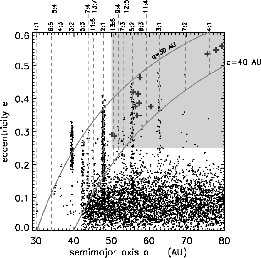
Figure 4: Eccentricity $e$ versus semimajor axis $a$ at time $t=4.5\times 10^{9}$ years for the model population having initial $e\sim 0.1$ shown in Fig. 3. The vertical dashes indicate the mean motion resonances that are occupied by trapped particles with perihelia $q<40$ AU or particles inhabiting resonances in the gray region with libration amplitudes $|\phi_{jk}|\leq 90^{\circ}$. Crosses indicate scattered particles.

Figure 3 also shows that trapping at the distant high–order resonances like the 5:2 and 3:1 is quite effective at promoting bodies into eccentric orbits having $a\gtrsim 50$ AU and perihelia $30\lesssim q\lesssim 40$ AU. This domain is usually regarded as the Scattered Disk. This result then suggests the possibility that some of the observed KBOs in the $30\lesssim q\lesssim 40$ AU zone may actually be resonantly trapped bodies that are masquerading as members of the Scattered Disk. Of course, particles scattered by Neptune also tend to spend a large fraction of their time near resonances due to the resonance sticking phenomenon (e.g., Duncan & Levison 1997; Malyshkin & Tremaine 1999). Therefore, the discrimination between scattered and resonantly trapped particles must be done carefully. Towards this end, we examine the orbital histories of all surviving particles in the shaded zone in Fig. 4 that have $e>0.25$ and $a>50$ AU. The usual definition of being ‘in’ a $j+k:j$ mean motion resonance is that the particle’s resonance angle $\phi_{jk}$, Eqn. (A1), librates about some fixed value with some modest amplitude $|\Delta\phi_{jk}|$ that is usually $\lesssim 90^{\circ}$, while the resonance angle for a scattered body that is temporarily ‘stuck’ in a resonance will have a $\phi_{jk}$ that circulates over $\pm 180^{\circ}$. However, we find that $|\Delta\phi_{jk}|$ is not the best discriminant for identifying trapped and scattered particles because a small but significant fraction of particles do get trapped at a resonance with a $\phi_{jk}$ that is either circulating or else librating with a very large amplitude. For some trapped particles, this distinction is unclear due to this simulation’s infrequent time–sampling that occurs every $\Delta t=10^{8}$ years.

Rather, a more reliable discriminant between trapped and scattered particles is based on Brouwer’s integral $B$, Eqn. (A6). This integral is conserved by resonantly trapped particles but is not conserved by scattered particles that are temporarily exhibiting the ‘resonance sticking’ phenomenon. Of the 134 particles that inhabit the gray zone in Fig. 4, only 12, or about $10\%$ of these particles, are truly scattered particles whose orbits $(a,e)$ evolve stochastically about the $30\lesssim q\lesssim 40$ AU zone; these scattered particles are indicated by the crosses in Fig. 4. The remaining particles are resonantly trapped particles, most of which preserved their $B$ integral to within $\sim 3\%$.

The orbits of all particles having perihelia $q<40$ AU have also been inspected, and those resonances inhabited by trapped particles having libration amplitudes $|\phi_{jk}|\leq 90^{\circ}$ are indicated by the vertical dashes in the Figure. We find that particles get trapped at a number of exotic resonances like the 11:6, 13:7, 13:6, 9:4, 12:5, 8:3, and the 11:4.

5 Kuiper Belt inclinations

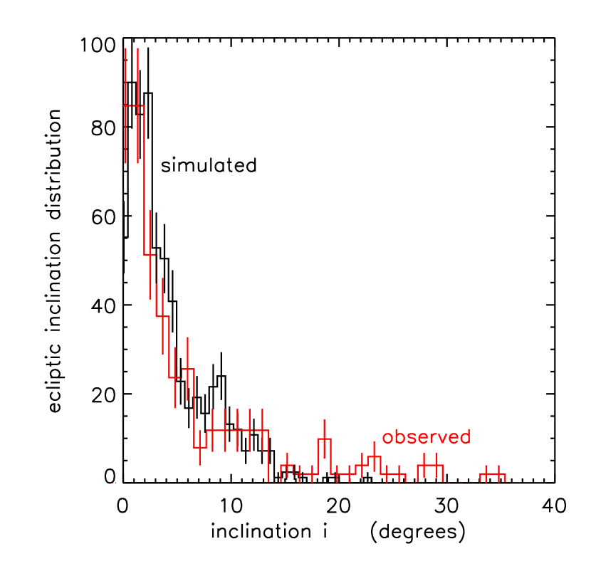
Figure 5: The ecliptic inclination distributions for the simulated and observed bodies in Fig. 3 that have perihelia $q<42$ AU and latitudes $|\beta|\leq 1^{\circ}$. Error bars give the Poisson counting uncertainty, and the vertical scale is arbitrary.

Inspection of the inclinations shown in Fig. 3 suggests that the smooth migration model does not produce sufficient numbers of bodies in high–inclination orbits. This has been recognized in previous studies (Malhotra 1995; Gomes 1997), but has not been quantified. However one should not directly compare the simulation’s $i$’s to the observed KBO inclinations, since the latter is heavily biased by telescopic selection effects. Note that most telescopic surveys of the Kuiper Belt observe near the ecliptic, which favors the discovery of lower–$i$ KBOs that spend a larger fraction of their time at lower latitudes (Jewitt & Luu, 1995). To mitigate this selection effect, one should instead consider the ecliptic inclination distribution, which is the inclination distribution of objects having latitudes $\beta$ very near the ecliptic (e.g., Brown 2001). The ecliptic inclination distribution for multi–opposition KBOs having perihelia $q\leq 42$ AU and latitudes $|\beta|\leq 1^{\circ}$ (red curve) is shown in Fig. 5, as well as the simulated ecliptic inclination distribution for particles from Fig. 3 that are selected similarly (black curve).

The agreement seen in Fig. 5 among bodies having inclinations of $0\lesssim i\lesssim 15^{\circ}$ shows that the smooth migration model can readily recover the Kuiper Belt’s lower inclination members. Of course, this agreement is partly due to the particles’ initial inclinations being distributed around $\langle i\rangle\simeq 3^{\circ}$. But Fig. 5 also shows this model to be quite deficient in producing sufficient numbers of the high–$i$ bodies having $i\gtrsim 15^{\circ}$. Similar results are also obtained among bodies orbiting at Neptune’s 3:2 resonance. This is a serious discrepancy, since Brown (2001) has shown that there are two inclination–populations in the Kuiper Belt: a minor population of low–$i$ having characteristic inclinations of $i\sim 3^{\circ}$, and a high–$i$ population having $i\sim 15^{\circ}$ containing about three–quarters of all KBOs. Note that these high–$i$ bodies are very underrepresented in Fig. 5 due to telescopic selection effects.

Of course, Neptune–scattered particles routinely achieve high inclinations of $i\gtrsim 15^{\circ}$; for instance, many of the high–$i$ particles seen in Fig. 2 were scattered by Neptune. Could the Scattered Disk be a source of the high–$i$ KBOs that are found elsewhere in the Belt? Recent Nbody simulations by Gomes (2003) show that a small fraction of these Neptune–scattered particles can evolve from very eccentric, Neptune–crossing orbits into less eccentric orbits in the Main Belt. In Gomes’ simulations, this occurs principally at secular and mean motion resonances that drive large oscillations in a scattered particle’s eccentricity. When a scattered particle visits a resonance, it can have its $e$ temporarily lowered and its $q$ raised. If this occurs during the planet–migration epoch, this process becomes irreversible and can strand Scattered particles in the Main Belt with their high inclinations. Such bodies are identified by Gomes as ‘evaders’ since they are Neptune–crossing bodies that ultimately manage to evade Neptune when deposited in the Main Belt. Note, however, that the efficiency of this process is quite low, affecting only $\epsilon\sim 0.002$ of all Scattered particles in the simulation that is evolved over the age of the Solar System by Gomes (2003). However all of the high–$i$ particles seen in our simulation (Fig. 3) achieved their inclinations while temporarily or permanently trapped in Neptune’s advancing resonances. There were no Neptune–scattered evaders having $i>10^{\circ}$ that survived in our simulations.

Despite the evader mechanism’s inefficiency, a model can still be constructed that yields a KBO inclination distribution that is quite similar to the observed one. For instance, this can be achieved by making the number density of small bodies initially orbiting interior to $\sim 27$ AU about 60 times higher than the density of bodies initially orbiting beyond 27 AU. As Gomes (2003) show, Neptune’s migration through this densely–populated inner disk creates the Kuiper Belt’s high–$i$ evaders, while the sparse outer disk provides the Belt’s low–$i$ component. Although this scheme yields an $i$–distribution that does indeed agree with the observations, that success is achieved via a special configuration of the initial particle disk.

However, Levison & Morbidelli (2003) avoid this problem of special initial conditions by assuming that the initial planetesimal disk simply ended at $\sim 35$ AU. This is the ‘push–out’ model, which argues that most of the Kuiper Belt is a consequence of Neptune’s advancing 2:1 resonance, which can drag bodies outwards to litter the Main Belt with low–$i$ KBOs. The Belt’s high–$i$ component is then presumed to be due to the evader mechanism. While the push–out model remains quite intriguing, it would be interesting to see this scenario subjected to greater scrutiny to see whether it can indeed reproduce the Kuiper Belt’s curious mix of high and low inclination KBOs in a self–consistent manner.

6 A Kuiper Belt census: comparison with observations

Figure 6 plots the relative abundance, over time, of the simulated Belt’s various dynamical classes among particles having perihelia $q\leq 45$ AU. These curves are normalized such that the final abundance of the Main Belt (MB), where $40.1\leq a\leq 47.2$ AU, is unity. Note that this model predicts a 2:1 resonance that is 1.4 times more abundant than the Main Belt, and 2.5 times more abundant than the 3:2, while the observations (Fig. 3) show a 2:1 that is only sparsely populated. Of course, when comparing the simulated population to the observed population, one must first deal with the observational selection effect that strongly favors the discovery of larger and/or nearer KBOs. However it is shown below that the effects of this bias can be accounted for by using a Monte Carlo method that assigns random sizes to the simulated population. This then allows one to make a fair comparison of the relative abundances of the simulated and observed populations.

Begin by letting $N(R)=$ the number of bodies in the simulated population having radii exceeding a radius $R$. Also let $\xi$ be a random number that is uniformly distributed between zero and one, and interpret this number as the probability of selecting a body with a radius that is smaller than $R$. This is also equal to the probability of not selecting a body of radius $>R$, so $\xi=1-N(R)/N_{total}$ where $N_{total}$ is the total number of bodies in this population. Since most small–body populations have a cumulative size distribution $N(R)$ that varies as a power law, adopt

$$N(R) = N_{total}\left(\frac{R}{R_{min}}\right)^{-Q}$$ (4)

where $R_{min}$ is the radius of the smallest member of the swarm. Then $R/R_{min}=(1-\xi)^{-1/Q}$, but $1-\xi$ can be replaced with $\xi$ since these random numbers have the same distribution, so

$$R(\xi) = \frac{R_{min}}{\xi^{1/Q}}.$$ (5)

Equation (5) is then used to generate random sizes for the simulated population of Fig. 3 that have apparent R–band magnitudes of

$$m_{R}=m_{\odot}-2.5\log\left[p\left(\frac{R}{r_{1}}\right)^{2}\left(\frac{r}{r_{1}}\right)^{-2}\left(\frac{r-r_{1}}{r_{1}}\right)^{-2}\right]$$ (6)

where $r$ is the particle’s heliocentric distance, $r_{1}=1$ AU, $m_{\odot}=-27.29$ is the Sun’s apparent $R$ magnitude, $R_{min}=20$ km is adopted here, and the observation is presumed to occur at solar opposition. All of our calculations will also adopt the usual albedo of $p=0.04$ so that our findings can be readily compared to past results obtained by others. However if an alternate albedo $p$ is desired, simply revise all KBO radii reported here by a factor of $(p/0.04)^{-1/2}$, and all masses by a factor of $(p/0.04)^{-3/2}$. Finally, note that a power–law size distribution results in a cumulative luminosity function that varies as $\Sigma(m)\propto 10^{\alpha m}$, where $\Sigma(m)$ is the sky–plane number density of KBOs brighter than apparent magnitude $m$ and the logarithmic slope is $\alpha=Q/5$ (Irwin et al., 1995).

Hubble Space Telescope observations reveal that the bright end of the Kuiper Belt’s luminosity function has a steep logarithmic slope of $\alpha=0.88\pm 0.1$ for bodies having magnitudes $m_{R}\ll 24$, while the faint end ($m_{R}\gg 24$) of the luminosity function has a shallow logarithmic slope of $\alpha=0.32\pm 0.15$ (Bernstein et al., 2004); the steeper slope of the bright end of the luminosity function was also confirmed recently by Elliot et al. (2005). This luminosity function can be interpreted as evidence that the KBO size distribution is actually two power laws that break even at a magnitude $m_{break}\simeq 24$, which corresponds to a body of radius $R_{break}\simeq 65$ km orbiting at a characteristic distance of $r\sim 40$ AU assuming it has an albedo of $p=0.04$. However our application will concentrate only on those KBOs that have known orbits, and $99\%$ of those bodies have magnitudes $m_{R}<m_{break}$. Consequently, this study will be sensitive only to the larger end of the KBO size spectrum, and such bodies will be characterized here via a single power–law size distribution having $\alpha=0.88$ and $Q=5\alpha=4.4$.

Although $\sim 5000$ simulated particles in Fig. 3 manage to survive over the age of the Solar System, the Monte Carlo model assigns far too few of them with sizes that would be detected by any telescopic survey of the Kuiper Belt. To boost the statistics of the detectable portion of the simulated population, each survivor is replicated $10^{4}$ times such that each particle’s orbit elements $a,e,i,\Omega,\omega$ are preserved while its mean anomaly $M$ is randomly distributed over $0\leq M<2\pi$. It should be noted that this step effectively assumes that the particles’ longitudes are uniformly distributed over $2\pi$, which is not quite correct since Neptune’s resonant perturbations tend to arrange the particles’ longitudes in a non–uniform manner (Malhotra, 1996; Chiang & Jordan, 2002). Nonetheless, this is not a major concern since the observed KBOs were discovered along lines–of–sight that are roughly distributed uniformly in ecliptic longitude, which effectively washes–out Neptune’s azimuthal arrangement of the Belt; see Appendix C for a more detailed examination and justification of this assumption. Lastly, this Monte Carlo model is then tested by verifying that the randomly generated population does indeed exhibit the expected luminosity function that varies as $\Sigma(m)\propto 10^{Qm/5}$.

Further comparison of the Monte Carlo model of the Kuiper Belt to any observations must be done carefully. Note that the brighter KBOs tend to be discovered in shallow, wide–angle surveys that observe a large area $\Delta\Omega$ on the sky, while the fainter KBOs tend to be discovered in deeper surveys that observe smaller areas $\Delta\Omega$. Consequently, the observed abundances of the various KBO subclasses (e.g., the Main Belt, the Scattered Disk, etc.) are proportional to all of these surveys’ total area $\Omega(m_{R})$, which itself is some function of the limiting magnitude $m_{R}$. However Appendix B shows that this dependence upon $\Omega(m_{R})$ can be factored out by constructing ratios of the Belt’s various subclasses. That Appendix also shows that the ratios of the observed abundance of any two dynamical classes of KBOs is approximately equal to the ratio of the intrinsic abundances of the much larger unseen populations. Thus by plotting ratios of the simulated populations to the observed KBO populations, we can compare the model to the observations in a manner that is insensitive to survey details like their individual sky–coverage $\Delta\Omega$.

Figure 7 shows the apparent abundances of the 2:1 and the 3:2 populations relative to the Main Belt (MB) as a function of their $R$–band magnitudes $m_{R}$. The upper light gray curve is the simulated ratio, which predicts an apparent 2:1 abundance that is about $80\%$ of the MB, while the dark gray curve is the observed ratio. Taking the ratio of these two curves reveals that their discrepancy at magnitudes $m_{R}>21$ (which refers to about 90% of the observed sub–populations) is a factor of $f_{2:1}\simeq 20$—the observed 2:1 resonance is markedly underabundant relative to the observed Main Belt population. There are $N_{MB}(R>50\mbox{ km})=1.0\times 10^{5}$ Monte Carlo particles in the simulated Main Belt having radii $R>50$ km, and $N_{2:1}(R>50\mbox{ km})=8.2\times 10^{4}$ particles in the 2:1. If we let $r_{2:1/MB}$ represent the inferred ratio of 2:1 to Main Belt objects, then $r_{2:1/MB}\simeq N_{2:1}/f_{2:1}N_{MB}\simeq 0.041$, which is comparable (albeit lower by a factor of $\sim 2$) to the ratio that Trujillo et al. (2001) infer from telescopic surveys of the Kuiper Belt.

The observed 3:2/MB ratio plotted in Figure 7 also shows that this resonant population is underabundant relative to model predictions by a factor of $\sim 6$ among bright objects with $21\lesssim m_{R}\lesssim 23$, and by a factor of $\sim 60$ at fainter magnitudes. Close inspection of the observations suggests that there indeed is a deficiency of fainter KBOs in the 3:2, and that this curve is not due to some overabundance of Main Belt KBOs having magnitudes of $m_{R}\simeq 23$.

It should be noted that the results given in Fig. 7 are not particularly sensitive to the detailed location of the Main Belt’s outer edge. For instance, if we assumed the Belt’s primordial edge where instead at $a=45$ AU (e.g., Trujillo & Brown 2001; see also Section 7), this reduces the 2:1 and MB populations both by about 40% while leaving the 3:2 population unchanged. Consequently, the 2:1/MB ratios of Fig. 7 are largely unchanged for both the simulated and observed populations, while the 3:2/MB ratios increase by a factor of $(1-0.4)^{-1}\simeq 1.7$. However the discrepancy between the simulated and observed populations is still the same factors of $\sim 6$–60.

Although there are several possible interpretations of the discrepancies seen Fig. 7, the most plausible explanation is that other unmodeled processes are responsible for (i.) reducing the trapping efficiencies of the 2:1 and 3:2 resonances by factors of $\sim 6$–60, or (ii.) causing trapped particles to diffuse out of the resonances and into nearby regions of phase space that are quite unstable (cf. Fig. 1 of Duncan et al. 1995), resulting in their ejection from the Kuiper Belt. Such unmodeled processes include the collisions and gravitational scatterings that occurred with ever greater vigor during earlier times when the Belt was more crowded. The scattering of these planetesimals by Neptune was of course responsible for driving that planet’s migration, so the occasional scattering of a large and/or close planetesimal will cause that planet’s orbit and hence its resonances to shudder some. Likewise, scattering events among the KBOs themselves would also cause their semimajor axes to diffuse some, as would collisions. This means that scatterings and collisions will have driven a random walk in the resonant particles’ semimajor axes, as well as a random walk in the location of the resonances themselves. It is possible then that these unmodeled effects can drive particles out of resonances and reduce the resonant population by the large factors indicated by Fig. 7, a scenario that is also explored in simulations by Zhou et al. (2002) and Tiscareno & Malhotra (2004).

The magnitude dependence of the observed 3:2/MB ratio shown in Fig. 7 is also quite curious. The fact that the observed ratio varies with apparent magnitude $m_{R}$, while the simulated ratio remains constant at magnitudes fainter than $m_{R}=21$, suggests that the $N(R)\propto R^{-Q}$ power–law that was universally applied throughout the entire Belt is overly simplistic. One way for the model to achieve better agreement with the observations is to assume that larger, brighter bodies are more abundant in the 3:2, and that smaller, fainter bodies are less abundant there than they are in the MB, which requires a shallower size distribution. The dashed curve in Fig. 7 illustrates this possibility, which shows the simulated 3:2/MB ratio assuming that the 3:2 bodies have a shallow $Q=2.7$ size distribution with $R_{min}=4.3$ km (note that reducing $R_{min}$ has the effect of reducing the total number of visible objects) while the MB bodies have the usual distribution with $Q=4.4$ and $R_{min}=20$ km. The shallow size distribution that is inferred here for the 3:2 population is also consistent with the logarithmic slope of $\alpha\simeq 0.56$ that Elliot et al. (2005) recently reported for the luminosity function of their ‘resonant’ population that is dominated by 3:2 KBOs; the size distribution inferred from that work is $Q=5\alpha=2.8$. KBO sizes can also vary with inclination [Levison & Stern (2001), but see also footnote 1 of Gomes (2003)]. In particular, Bernstein et al. (2004) report that the bright end of the luminosity function for high–inclination ($i>5^{\circ}$) KBOs have a logarithmic slope of $\alpha=0.66$ and a size distribution $Q=5\alpha=3.3$ that is much shallower than the low–$i$ KBOs having $\alpha=1.36$ and a $Q=5\alpha=6.8$.

In our Monte Carlo model there are only $N_{3:2}(R>50\mbox{ km})=2100$ bodies larger than $R=50$ km, so their numerical abundance relative to the Main Belt is $r_{3:2/MB}=N_{3:2}/N_{MB}=0.021$, which again is comparable (but again lower by a factor of $\sim 2$) to the ratio reported in Trujillo et al. (2001). The largest Monte Carlo body at the 3:2 has a radius $R\simeq 1000$ km, which is comparable to the size of the largest multi–opposition KBO there with $R\simeq 1100$ km, assuming $p=0.04$.

This range of power–law indices that is inferred for the Kuiper Belt, $2.7\lesssim Q\lesssim 4.4$, is comparable to the values of $Q$ that are observed at various sites throughout the asteroid belt. The Near Earth Objects have a fairly shallow size distribution with $Q=1.95$ (Stuart & Binzel, 2004), while the asteroid families exhibit steeper size distributions. For instance, Fig. 1. of Tanga et al. (1999) shows size distributions for several prominent asteroid families having values of $2\lesssim Q\lesssim 6$. Note also that nonfamily asteroids have $Q\simeq 3.0$ (Ivezić et al., 2001), which is slightly steeper than the canonical $Q=2.5$ value that results from a collisional cascade (Dohnanyi, 1969). Since the various asteroid subclasses exhibit such a wide variation in their size distributions over a relatively narrow range of semimajor axes of $\Delta a\sim 4$ AU, perhaps it should be of no surprise that the spatially much wider Kuiper Belt might also exhibit some variety in $Q$.

7 The outer edge of the Solar System

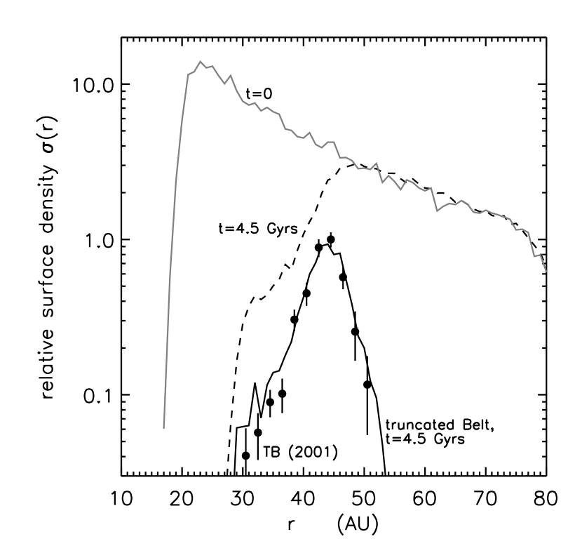
Figure 8: Dots show the KBO surface number density $\sigma(r)$, normalized to peak at unity, that is inferred from the KBOs radial distribution function $f(r)\propto r\sigma(r)$ reported by Trujillo & Brown (2001). The $t=0$ and $4.5$ Gyr curves are the simulated Belt’s initial and final surface density. The ‘truncated Belt’ curve is the simulation’s final surface density assuming that the Belt is truncated at $a=45$ AU, and that the 3:2 population also does not contribute to $\sigma$. Note that the surface density of the inner half of this Belt increases as a very steep function of distance as $\sigma(r)\propto r^{9.5}$ for $r\lesssim 45$ AU.

Inspection of Figure 3 shows a prominent absence of observed KBOs having modest eccentricities of $e\sim 0.1$ near and beyond Neptune’s 2:1 resonance. The prevailing interpretation of this observed feature is that there is a boundary near $45\lesssim a\lesssim 50$ AU that marks the outer edge of the Solar System’s primordial Kuiper Belt (Allen et al., 2001; Trujillo & Brown, 2001). The dots in Fig. 8 shows the Belt’s surface density $\sigma(r)$ that is inferred from these observations, which peaks at $r\simeq 45$ AU. We have nonetheless allowed our simulated Kuiper Belt to extend out to $a=80$ AU in order to use the dearth of observed distant KBOs to place quantitative upper limits on the abundance of hypothetical KBOs that might live beyond 50 AU.

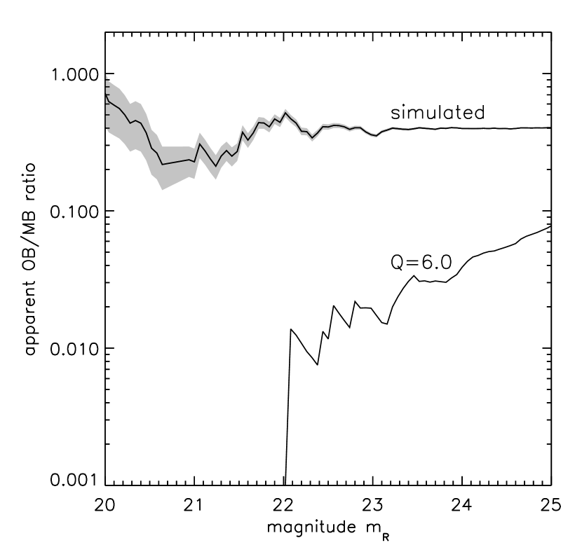
Figure 9: The gray curve is the expected ratio of bodies in the Outer Belt (OB, beyond $a>50$ AU) relative to the Main Belt (MB, $40.1<a<47.2$ AU) as a function of magnitude $m_{R}$ assuming the size distribution has $Q=4.4$ and $R_{min}=20$ km. The solid curve is the OB/MB ratio assuming the OB instead has a steeper $Q=6.0$ size distribution while the MB has $Q=4.4$, with $R_{min}=20$ km for both populations.

The Nbody/Monte Carlo of the previous Section can be used to predict how many KBOs should have been observed in the $a>50$ AU zone (which we identify here as the Outer Belt, or OB) assuming (i.) that the primordial Kuiper Belt extends smoothly out to $a=80$ AU, and (ii.) that all KBOs everywhere have the same size distribution with the usual parameters $Q=4.4$ and $R_{min}=20$ km. This simulation’s ratio of Outer Belt/Main Belt objects, $r_{OB/MB}(m_{R})$, is plotted versus magnitude $m_{R}$ in Fig. 9. This is the ratio of $N^{sim}_{OB}(m_{R})=$ the number of bodies in the simulated Outer Belt (whose members have semimajor axes $50<a<80$ AU and eccentricities $e<0.2$), to $N^{sim}_{MB}(m_{R})=$ the number of bodies in the simulated Main Belt (where $40.1<a<47.2$ AU) in the magnitude interval $m_{R}\pm\Delta m$ where $\Delta m=0.5$. According to the Figure, the expected OB/MB ratio is $r_{OB:MB}=0.4$. At present there are $N^{obs}_{MB}=264$ KBOs in the MB that have been observed for 2 or more oppositions, and the dimmest member of this group of KBOs has an apparent magnitude $m_{R}^{\star}=24.5$. The Nbody/Monte Carlo model thus predicts that there should also be $N^{obs}_{OB}=r_{OB/MB}N^{obs}_{MB}\simeq 100$ objects brighter than $m_{R}^{\star}$ orbiting in the OB beyond $a=50$ AU. This prediction is in marked contrast with the observations which show that there are no known multi–opposition objects orbiting in the OB with magnitudes brighter than $m_{R}^{\star}$, i.e., $N^{obs}_{OB}<1$.

This prediction that the Outer Belt would have an observed abundance that is $40\%$ of the Main Belt differs considerably from that of Gladman et al. (1998) who estimated that the observed Outer Belt population should only be $\sim 6\%$ of the total observed population. However this much lower estimate was obtained by assuming that the current Belt’s surface number density resembles its primordial $\sigma(r)$ which likely varied as $r^{-2}$ or so. This very common assumption causes the inner part of the Belt to be more concentrated than its outer part. However a real Kuiper Belt has been dynamically eroded over the eons by the giant planets’ gravitational perturbations. This dynamical erosion is illustrated in Fig. 8, which shows the simulated Belt’s primordial surface density (gray curve) and its final surface density (dashed curve); similar erosion is also seen in the long–term integrations of Duncan et al. (1995). Figure 8 shows that $\sigma(r)$ for an eroded Belt is a sharply increasing function of $r$ for $r\lesssim 50$ AU, which implies that the inner observable portion of the Belt is very underdense relative to the more distant $r\sim 50$ AU zone. This dynamical erosion accounts for the discrepancies between our Outer Belt predictions and that by Gladman et al. (1998).

Recall that Figs. 3 and 7 show that the 2:1 and 3:2 populations are very depleted relative to model predictions, and that the zone beyond Neptune’s 2:1 resonance is either empty or inhabited by bodies too small and faint to be seen. To account for these depletions, the solid curve in Fig. 8 also shows a revised surface density curve that is obtained from the simulated Belt that is truncated at $a=45$ AU (about 3 AU inwards of Neptune’s 2:1 resonance), and with the negligible contribution from the 3:2 populations also being ignored. This result is a curve that agrees quite well with the Belt’s observed surface density variations. Despite this good agreement in the radial distributions of the simulated and observed Kuiper Belts, Fig. 3 shows that this apparent edge at $a=45$ AU is still rather fuzzy since there are four multi-opposition KBOs of low eccentricity ($e<0.05$) orbiting in the Main Belt at $45<a<48$ AU. Close inspection of Fig. 3 shows that a hard edge at $a=45$ AU also could not account for the KBOs having $e\sim 0.1$ in the $45<a<48$ AU, unless the advancing 2:1 resonance also dragged some bodies out of the $a<45$ AU zone and deposited them here, reminiscent of the scenario suggested by Levison & Morbidelli (2003).

The remainder of this Section places upper limits on the size and abundance of any unseen KBOs that might lurk beyond $a=50$ AU. Of course there are multiple interpretations of the dearth of observed multiple–opposition bodies orbiting beyond $a=50$ with modest eccentricities of $e\sim 0.1$, i.e., that $N^{obs}_{OB}<1$. One interpretation of this upper limit is that assumption (i.) is incorrect—that the primordial Kuiper Belt’s density did not extend smoothly beyond Neptune’s 2:1, but that it instead was reduced by a factor $f$ (relative to the smooth model’s density) in the $a>50$ AU zone. In this case, the OB/MB ratio becomes $r_{OB/MB}=0.4/f=N^{obs}_{OB}/N^{obs}_{MB}<1/N^{obs}_{MB}$, which implies that the primordial density of the OB was smaller than the MB by a factor $f\gtrsim 100$.

Alternatively, assumption (ii.) could be incorrect, namely, that the KBO size distribution was not uniform everywhere. For instance, the absence of any multi–opposition bodies in the OB having magnitudes brighter than $m_{R}^{\star}=24.5$ could simply mean that bodies beyond $r\simeq 50$ AU are dimmer than $m_{R}^{\star}$ and thus have radii smaller than $R\simeq 80(p/0.04)^{-1/2}$ km (see Eqn. 6). Note that Trujillo et al. (2001) obtained a similar limit, but that they came to regard this scenario as unlikely.

It is also possible that the Outer Belt’s size distribution is steeper, i.e., has a larger $Q$, than the Main Belt’s size distribution. An increase in $Q$ decreases the abundance of bright bodies, as is illustrated by the curve in Fig. 9 which gives the the $r_{OB/MB}$ ratio for an OB having a $Q=6.0$ size distribution while bodies in the MB have the usual $Q=4.4$ distribution. This particular $Q$ is also the minimum value that is consistent with the observed upper limit of $r_{OB/MB}<1/264$; Outer Belts with with a smaller $Q$ would contain at least 1 KBO brighter than $m_{R}^{\star}$ in the $a>50$ AU zone for every 264 KBOs detected in the Main Belt, while an OB having a larger $Q$ would be undetected. This particular model is near the threshold of detection, and its largest member has a radius of $R=250$ km. Trujillo et al. (2001) also considered this scenario, but they concluded that the absence of distant KBOs requires a steeper $Q>9$ size distribution. The origin of this discrepancy is unclear.

It is also interesting to note that the low–inclination KBOs have a logarithmic slope of $\alpha=1.36$ along the bright end of their luminosity function (Bernstein et al., 2004), which implies a steep size distribution of $Q=5\alpha=6.8$. Such bodies, if they inhabit the Outer Belt beyond $a=50$ AU with the same abundances as adopted by our model, could conceivably have avoided detection to date due to their steep size distribution. In other words, a Main Belt whose low–$i$ population extends beyond $a=50$ AU while its high–$i$ population terminates at $a=50$ AU could be quite consistent with their non–detection.

From these considerations it may be concluded that the observed absence of multi–opposition KBOs in the $a>50$ AU zone having modest eccentricities $e\sim 0.1$ implies: (i.) that this part of the primordial Kuiper Belt was underdense by a factor of $f\gtrsim 100$ relative to the $a<50$ AU zone, or that (ii.) these distant KBOs have radii $R\lesssim 80$ km, or that (iii.) their size distribution has a power–law index $Q>6.0$, or perhaps (iv.) some combination of the above effects.

8 The origin of Centaurs

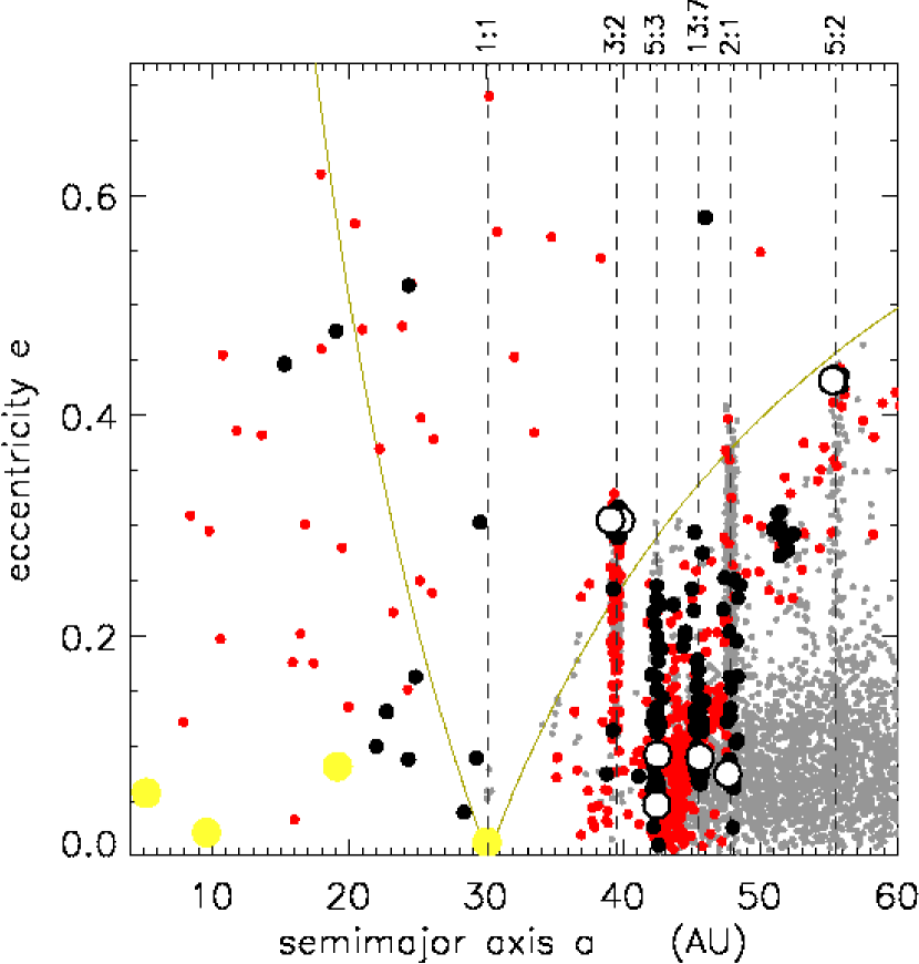
Figure 10: Open circles are the orbits of the simulation’s seven Centaurs at time $t=10^{8}$ years, while black dots indicate their subsequent motions. Gray dots are the simulation’s endstate at time $t=4.5\times 10^{9}$ years, red dots indicate multi–opposition KBOs and Centaurs, and yellow dots are the giant planets’ final orbits. Neptune’s mean–motion resonances are indicated, and the curve is the threshold for Neptune–crossing orbits.

It is generally accepted that Centaurs are those bodies that have diffused inwards from the Kuiper Belt into orbits that cross the giant planets (e.g., Duncan et al. 1988). Presently there are 27 known Centaurs observed for more than one opposition; these are the red dots in Fig. 10 having $a<30$ AU. Since planet–crossers are quickly ejected or accreted, Centaurs have short dynamical lifetimes of only $\sim 10^{7}$ years (Levison & Duncan, 1997; Tiscareno & Malhotra, 2003). Consequently, the density of these ‘escapees from the Kuiper Belt’ (e.g., Stern & Campins 1996) is very tenuous inside of $a=30$ AU (see Fig. 8). Indeed, only $N_{C}^{\star}=7$ Centaurs are detected during the final $\Delta T=2$ billion years of our simulation that was only sparsely time–sampled once every $\Delta t=10^{8}$ years, so the instantaneous number of Centaurs is $N_{C}=N_{C}^{\star}(\Delta t/\Delta T)=0.35$ at the end of the simulation. There are also $N_{MB}=565$ bodies in the Main Belt, so the Centaur/Main Belt ratio is provisionally estimated at $r_{C/MB}=6.2\times 10^{-4}$.

The open circles on Fig. 10 show the orbital elements of these seven Centaurs at time $t=10^{8}$ years, which is at a time when planet migration has only recently ceased. Thus the open dots indicate the locations where Neptune has parked these proto–Centaurs in the Kuiper Belt. Note that all seven Centaurs originate from sites in/near Neptune’s mean–motion resonances, namely, the 3:2, 5:3, 13:7, 2:1, and the 5:2. Their subsequent motions at times $t>10^{8}$ years are shown as black dots (again, poorly time–sampled), which show that the eccentricities of nearly all proto–Centaurs initially wander up–and–down with constant $a$ until they have a close encounter with Neptune, scatter off that planet, make a brief apparition in the $a<30$ AU Centaur zone, and then are quickly removed from the system.

These seven bodies have initial semimajor axes of $28\leq a\leq 48$ AU at time $t=0$, so Centaurs can also be regarded as samples that have been drawn from a wide swath of the outer solar nebula. Fig. 10 also shows that the simulated Centaurs are concentrated just inside of Neptune’s orbit; their mean heliocentric distance is $r=26\pm 3$ AU, and their mean inclination is $i=16\pm 10^{\circ}$. Note also that three of the seven Centaurs emerged from the 3:2 and 2:1 resonances, which Section 6 showed to be heavily depleted relative to the model’s predictions. Consequently, the Centaur/Main Belt ratio reported above should instead be interpreted as an upper limit, e.g., $r_{C/MB}<6.2\times 10^{-4}$. It is shown later in Section 11 that our model predicts that there are $N_{MB}\simeq 1.3\times 10^{5}$ Main Belt KBOs having radii $R>50$ km, so this model also predicts that there are $N_{C}=r_{C/MB}N_{MB}<80$ similarly–sized Centaurs.

Although the Centaur upper limit reported here is comparable to the population that Sheppard et al. (2000) infer from the Centaur luminosity function, there is still a prominent disconnect in the heliocentric distances of the simulated and observed populations; our simulated Centaurs all reside at $r>22$ AU, while the three Centaurs that Sheppard et al. (2000) used to construct the Centaur luminosity were detected at heliocentric distances of $r<19$ AU. One possible interpretation of this excess of Centaurs at $r\lesssim 20$ AU is that Centaurs may be breaking up and spawning new Centaurs (e.g., Pittich & Rickman 1994) as they wander among the giant planets. Finally, we note that deep, wide–angle surveys of the Kuiper Belt, such as the Legacy Survey that is currently being implemented at the Canada France Hawaii Telescope, may soon reveal the existence of the more distant Centaurs that is anticipated by this model to reside at distances of $23\lesssim r\lesssim 29$ AU.

9 Neptune’s Trojans

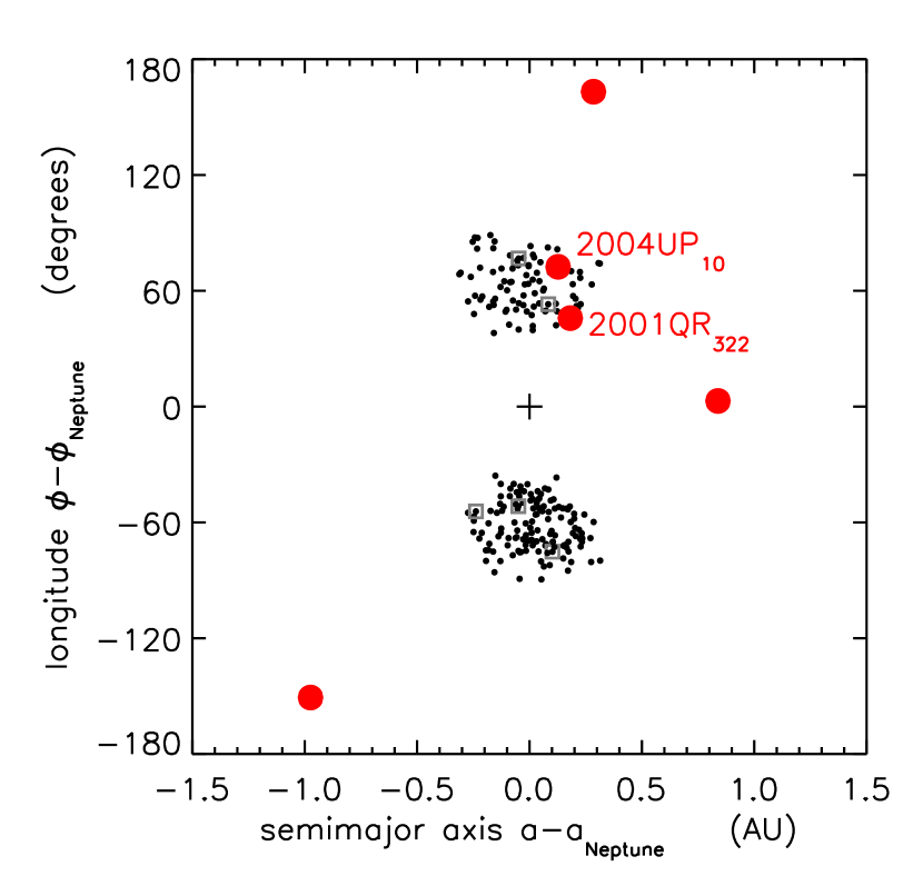
Figure 11: The black dots are the longitudes of five simulated trojans versus their semimajor axes, all relative to Neptune’s, and sampled every $10^{8}$ years during the entire simulation. Neptune lies at the $+$. Small squares show the final positions of these trojans, indicating that two trojans lie at the leading Lagrange point, with three trailing. Red dots indicate three nearby ‘field’ KBOs as well as Neptune’s two known Trojans, 2001 QR₃₂₂ and 2004 UP₁₀.

Figure 3 also shows that $N_{T}=5$ particles managed to survive the length of the simulation at Neptune’s 1:1 resonance. These simulated particles are of course Neptune’s Trojans, of which two are presently known: 2001 QR₃₂₂ (Chiang et al., 2003) and 2004 UP₁₀ (Sheppard et al., 2005). For this simulation the Trojan/MB ratio is $r_{T:MB}=N_{T}/N_{MB}=8.8\times 10^{-3}$, where $N_{MB}=565$ is the number of survivors that persist in the Main Belt. The spatial coordinates of the two observed and five simulated Trojans are shown in Figure 11, which indicates that these particles can roam about with longitudes of $\Delta\phi\simeq\pm 30^{\circ}$ from Neptune’s triangular Lagrange points with semimajor axes of $\Delta a\simeq\pm 0.32$ AU from Neptune’s. The extent of these Trojan sites are similar to that seen in integrations by Holman & Wisdom (1993) and Nesvorný & Dones (2002). Note that no special effort was made to start any of the simulated particles at Neptune’s Lagrange points. Rather, all particles were distributed randomly about a disk according to a smooth surface density law, with the inner edge of the disk being well inside of Neptune’s initial tadpole region. In our simulation the five survivors had initial semimajor axes of $\Delta a\simeq\pm 0.28$ AU from Neptune’s initial $a$, and there were a total of 68 particles initially in Neptune’s Trojan source region (i.e., $|\Delta a|\leq 0.28$ AU and $|\Delta\phi|\leq 30^{\circ}$), so the surviving Trojan fraction is about $7\%$. This survival fraction is comparable to that obtained by Kortenkamp et al. (2004) in a similar simulation. That work also showed that as planets migrate, several secondary resonances sweep across the 1:1, which result in a heavy loss of Neptune’s Trojans during the migration epoch.

Neptune’s Trojans are of interest since they might place constraints on some models of the early evolution of the outer Solar System. For example, Thommes et al. (1999, 2002) postulate that Neptune originally formed in the vicinity of Jupiter and Saturn and was tossed outwards after scattering off the larger planets. But the existence of 2001 QR₃₂₂ and 2004 UP₁₀ might cast doubt on this scenario since Trojans seem unlikely to persevere at Neptune’s Langrange during such a scattering event. However it has since been shown that a recently–scattered Neptune can still acquire its Trojans later as that planet’s orbit is circularized by a dense Kuiper Belt (Levison 2005, personal communication). It is also conceivable that Neptune may have captured its Trojan from a heliocentric orbit after Neptune’s orbit has settled down. Although Kortenkamp et al. (2004) shows that the direct capture of Trojans from heliocentric space is rare and results in only transient Trojans, Chiang & Lithwick (2005) show that mutual collisions may have inserted small bodies into stable orbits at Neptune’s Lagrange points after its orbit has circularized.

10 The Extended Scattered Disk

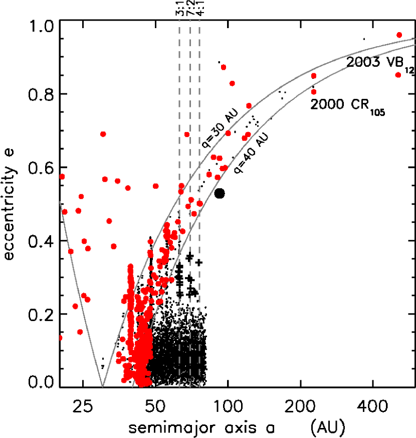
Figure 12: Eccentricities $e$ are plotted versus $a$ on a logarithmic axis for the particles of Fig. 3. Red dots are the KBOs observed over multiple oppositions, and the curves indicate the $q=40$ AU threshold as well as Neptune–crossing orbits. Two members of the so–called extended Scattered Disk, 2000 CR₁₀₅ and 2003 VB₁₂, are also indicated. Crosses indicate particles resonantly trapped at the 3:1, 7:2, and the 4:1. The large black dot indicates the only simulated particle that was scattered into a high–perihelia orbit ($q=43.5$ AU) that resembles 2000 CR₁₀₅.

Figure 12 shows the orbits of those scattered particles that have been tossed into very wide orbits about the Sun. Most of the simulated scattered particles have perihelia between $30\lesssim q\lesssim 40$, as do most of the observed scattered KBOs. However there are two exceptions to this rule, namely, 2000 CR₁₀₅ and 2003 VB₁₂ (also known as Sedna) which have respective perihelia of $q=44.14\pm 0.02$ (Gladman et al., 2002) and $q=76\pm 4$ AU (Brown et al., 2004). Gladman et al. (2002) classify those Scattered KBOs having perihelia higher than $q\simeq 40$ AU as members of a so–called extended Scattered Disk. Sedna’s large radius of $R\sim 1000$ km makes this object a particular curiosity since its discovery circumstance suggests that there may be a few hundred other unseen Senda–sized objects (Brown et al., 2004). Since Sedna has a mass of $\sim 10^{-3}$ M_⊕, the implied mass that might be hidden in the extended Scattered Disk is a few tenths of an Earth–mass. Thus Sedna by itself may represent an enormous reservoir of unseen mass that is comparable to the ‘conventional’ Kuiper Belt (see Section 11).

The extended Scattered Disk is also of dynamical interest since, as Gladman et al. (2002) note, most dynamical models of the Kuiper Belt (including this one) generally produce Scattered Objects in lower perihelia orbits having $q\lesssim 40$ AU. Gladman et al. (2002) review a number of scenarios that might explain how a KBO might get promoted from a nearly circular orbit into a wide, eccentric orbit having $q\gtrsim 40$ AU; these include: (i.) chaotic diffusion of scattered bodies, (ii.) gravitational scattering by long–gone massive protoplanets, (iii.) scattering by an undiscovered distant planet, and (iv.) scattering by a single star that passes to within $\sim 100$ AU of the Sun. However all of these scenarios are problematic. For instance, billion–year integrations of $\sim 10^{4}$ particles in chaotic Neptune–scattered orbits fail to diffuse into orbits having perihelia as high as that of 2000 CR₁₀₅ (Gladman et al., 2002). Morbidelli et al. (2002) also cast doubt on scenarios (ii–iii.) by showing that $\sim 20\%$ of any distant population of protoplanets would have persisted over the age of the Solar System, and that some fraction of these large bodies should already have been discovered by one of the various wide–angle Kuiper Belt surveys. Scenario (iv.) is also in doubt since simulations of a close encounter with a single star generally produce disturbances in an outer Kuiper Belt that is quite unlike that seen in the observed Belt (e.g., Ida et al. 2000). However Fernández & Brunini (2000) have shown that repeated encounters by more distant stars can produce Sedna–like orbits. This may have occurred early while the Sun was still a member of the open cluster from which it presumably formed. In this scenario, the giant planets scatter small bodies into wide orbits of $a\sim 100$ to 1000 AU, which the nearby cluster stars then perturb into Sedna–like orbits having higher perihelia. Scattering by a passing star was recently re–examined by Morbidelli & Levison (2004), and their simulations also support this scenario.

Although our simulations did not produce any Sedna–like objects in orbits that are well–decoupled from the giant planets, we did find a single scattered object in a 2000 CR₁₀₅–like orbit in the Extended Scattered Disk with a semimajor axis of $a=92$ AU and a perihelion of $q=43.5$ AU (the large black dot in Figure 12). The orbital history of this scattered particle is shown in Fig. 13, which shows that as the particle inhabited Neptune’s 16:3 resonance during times $2\lesssim t\lesssim 3$ Gyrs, some process raised this Scattered particle’s perihelion up and into the Extended Scattered Disk on a billion–year timescale. This kind of behavior was first reported in Levison & Duncan (1997) and Duncan & Levison (1997), whose simulations also show that some scattered particles can achieve high perihelia orbits while in or near mean–motion resonances.

However we have not identified any particular resonance as being responsible for raising the perihelia of our one CR₁₀₅–candidate shown in Fig. 13. For instance, a Kozai resonance is not implicated since the argument of perihelion $\omega$ does not librate. The possibility of other Pluto–like ‘super–resonances’ (e.g., Malhotra & Williams 1997) was also examined; this is the libration of a resonance angle of the form $\phi=j(\omega-\omega_{N})-k(\Omega-\Omega_{N})$, where $\Omega$ is the particle’s longitude of the ascending node and the $N$ subscript refers to Neptune’s orbit elements. Angles having $0\leq|j|,|k|\leq 10$ were examined, and although the angle $\phi=5(\Omega-\Omega_{N})$ angle did in fact librate for about 1 Gyrs, that occurred well after the time when the particle’s $q$ was raised. A resonance involving interactions with multiple planets is also unlikely since the particle’s Tisserand parameter $T$ (which is simply its Jacobi integral sans the interaction energy due to Neptune) was well–preserved during these times. Although the particular mechanism that drove this particle into the Extended Scattered Disk in not understood, this particle does demonstrate that it is indeed possible for Scattered particles to diffuse into the Extended Scattered Disk via planetary perturbations alone, with other external agents (like a stellar encounters) being absent. This transport from the Scattered Disk to the Extended Scattered Disk via mean–motion resonances is also evident in the simulations of Levison & Duncan (1997) and Duncan & Levison (1997). However this transport has an extremely low flux since only one of the $\sim 5\times 10^{3}$ particles initially in the Scattered Disk did manage to enter the Extended Scattered Disk and persist over the age of the Solar System. External perturbations from passing stars (Fernández & Brunini, 2000; Morbidelli & Levison, 2004) may indeed be more effective at producing members of the Extended Scattered Disk.

Note also the simulated particles represented by crosses in Fig. 12. Even though their perihelia of $42<q<54$ AU might suggest that they also inhabit the domain of the Extended Scattered Disk, they are in fact resonant particles that were trapped at the 3:1, 7:2, and 4:1 resonances during the migration epoch. Most of these particles have libration amplitudes less than $|\Delta\phi_{jk}|\lesssim 90^{\circ}$. These particles also had initial semimajor axes of ${a>47}$ AU, which is noteworthy since, if any resonant KBOs are ever discovered in these orbits, they could be interpreted as evidence that the outer edge of the Solar System lies beyond ${a>47}$ AU. However that interpretation would still be ambiguous, since Neptune–scattered evaders, which originated from smaller semimajor axes, can also settle into these same resonances—see Fig. 18 of Gomes (2003) for an example.

10.1 The Scattered Disk

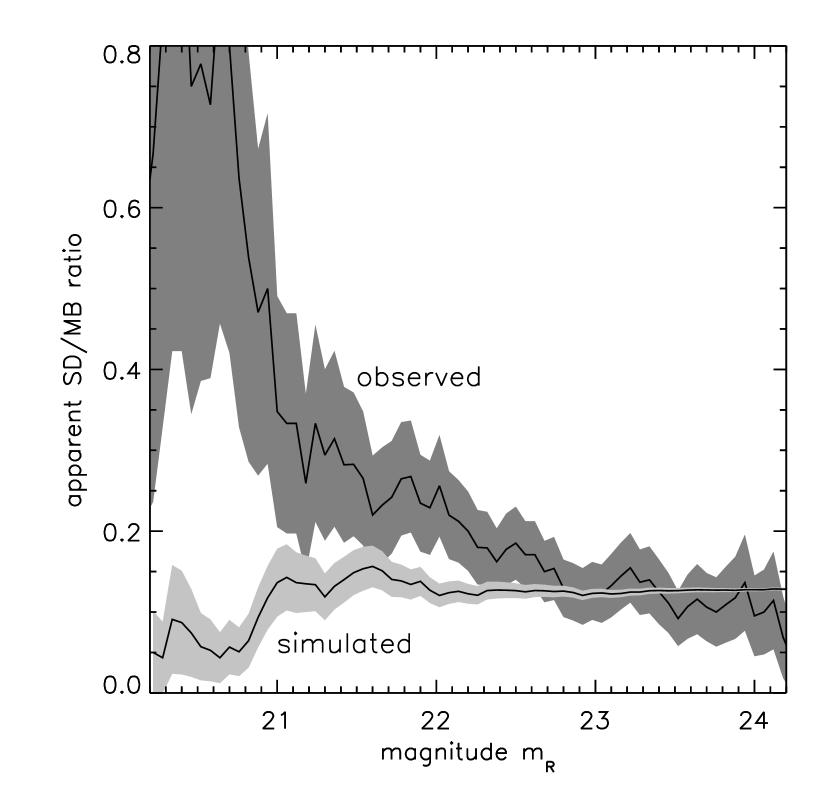
Figure 14: The dark gray curve is the observed ratio of Scattered Disk (SD) objects in orbits having $50<a<150$ AU and perihelia $28<q<40$ AU, relative to Main Belt (MB) objects, versus apparent magnitude $m_{R}$. The light gray curve is the simulated ratio.

Figure 14 shows the apparent abundance of so–called Scattered Disk objects relative to the Main Belt, as predicted by the Nbody/Monte Carlo model. There are $N_{SD}=1.9\times 10^{4}$ Monte Carlo bodies in orbits having $50<a<150$ AU and perihelia $28<q<40$ AU, while $N_{MB}=1.0\times 10^{5}$ Monte Carlo particles survive in the Main Belt, so the model predicts an intrinsic SD/MB ratio of $r_{SD/MB}=N_{SD}/N_{MB}=0.19$. The apparent ratio of these two populations is $\sim 0.1$, also shown in Fig. 14. Note that the intrinsic SD/MB ratio inferred here is about one–fourth that reported in Trujillo et al. (2001).

11 Calibration

The ecliptic luminosity function of Bernstein et al. (2004) is shown in Fig. 15, and its bright end varies as $\Sigma(m_{R})=10^{\alpha(m-m_{0})}$ deg^-2 where $\alpha=0.88$ and $m_{0}=23.1$, for magnitudes $m_{R}<m_{break}=24$. This luminosity function gives the number density of KBOs near the ecliptic that are brighter than magnitude $m_{R}$. Since this curve scales with the total number of KBOs, it can be used to calibrate the simulation to determine the total number of objects in the Kuiper Belt.

Sections 6–7 show that the observed 3:2 and 2:1 populations are severely depleted relative to model predictions, and that bodies in an Outer Belt beyond the 2:1 are either absent or too faint to be seen. To account for these depletions, the truncated Kuiper Belt similar to that of Section 7 is adopted; this Belt is formed by discarding any bodies orbiting beyond the 2:1, as well as all bodies orbiting within $\Delta a=0.6$ AU of Neptune’s 3:2 and 2:1 resonances. There are $N_{Nbody}=587$ Nbody particles in this truncated Kuiper Belt, and they are replicated $N_{reps}=10^{4}$ times with sizes and magnitudes assigned to them according to the Monte Carlo method of Section 6, with $Q=4.4$ and $R_{min}=20$ km.

The simulation’s median inclination is low (e.g., Section 5), only $\bar{i}_{sim}=2.7^{\circ}$, which is much lower than the median inclination $\bar{i}_{obs}=15.6^{\circ}$ that is inferred from the debiased KBO inclination distribution reported by Brown (2001). Due to these low inclinations, the simulation’s ecliptic luminosity function would thus be artificially overdense by a factor $f_{i}=\bar{i}_{obs}/\bar{i}_{sim}\simeq 5.8$, so it is revised downwards by this factor to compensate. The simulation’s $\Sigma(m_{R})$ is then multiplied by a factor $f_{N}=3.5$ to fit it to the bright end of the observed luminosity function; this accounts for the different populations in the simulated and observed Kuiper Belts, and results in the curve shown in Fig. 15. The size distribution adopted here is valid down to a radius of about $R_{break}=65$ km (see Section 6), so the inferred number of KBOs larger than $R_{break}$ is $N_{break}=N_{Nbody}N_{reps}f_{N}(R_{break}/R_{min})^{-Q}\simeq 1.1\times 10^{5}$. To estimate the total number of KBOs larger than the fiducial radius of $R_{50}=50$ km, note that the faint end of the observed luminosity function has a logarithmic slope of $\alpha_{faint}=0.32$ (Bernstein et al., 2004), which implies a power–law index of $Q_{faint}=5\alpha_{faint}=1.6$ for bodies having radii $R<R_{break}$. The total number of bodies larger than $R_{50}$ is thus $N_{50}=N_{break}(R_{50}/R_{break})^{-Q_{faint}}\simeq 1.7\times 10^{5}$.

The total mass of these bodies is obtained from their cumulative size distribution, which for the large bodies with $R>R_{break}$ can be written $N(R)=N_{break}(R/R_{break})^{-Q}$. The differential size distribution is then $dN(R)=|dN/dR|dR$, and if $M(R)=$ mass of a body having a radius $R$, the total mass of bodies having radii in the interval $R_{break}<R<R_{max}$ is

$$M(R>R_{break}) = \int_{R_{break}}^{R_{max}}M(R^{\prime})dN(R^{\prime})=\frac{Q}{Q-3}\left[1-\left(\frac{R_{break}}{R_{max}}\right)^{Q-3}\right]N_{break}M_{break}$$ (7)

where $M_{break}=M(R_{break})\simeq 1.2\times 10^{21}(\rho/\mbox{1 gm/cm${}^{3}$})(p/0.04)^{-3/2}$ gm, which is the mass of a body of radius $R_{break}=65$ km assuming it has a density $\rho$ and albedo $p$. The total mass of KBOs larger than $R_{break}$ with semimajor axes inside of Neptune’s 2:1 is thus $M(R>R_{break})\simeq 0.07(\rho/\mbox{1 gm/cm${}^{3}$})(p/0.04)^{-3/2}$ M_⊕ for a $Q=4.4$ size distribution that extends to radii as large as $R_{max}=1000$ km. To get the total mass of bodies at the fiducial size $R=R_{50}$, add to the above the mass of bodies in the size interval $R_{50}<R<R_{break}$, which is roughly $\Delta M\simeq(N_{50}-N_{break})M_{break}$. The total mass of bodies larger than $R_{50}=50$ km is then $M_{total}=M(R>R_{break})+\Delta M\simeq 0.08(\rho/\mbox{1 gm/cm${}^{3}$})(p/0.04)^{-3/2}$ M_⊕. Note that the $0.08$ M_⊕ prefactor is a consequence of adopting the oft–employed Halley albedo of $p=0.04$. However recent observations indicate KBOs have an average albedo of $p\simeq 0.1$ (Altenhoff et al., 2004; Grundy et al., 2005), which in turn lowers the Kuiper Belt mass to $M_{total}\sim 0.02$ M_⊕ assuming they have a unit density.

This population estimate is comparable to, but a bit higher than, previous estimates that rely on far simpler models of the Kuiper Belt. For instance, Trujillo et al. (2001) report a Main Belt population of $3.8\times 10^{4}$ objects of mass $0.03$ M_⊕ among bodies having radii $R>50$ km. They also estimate the Belt’s total population to be $1.9\times$ the Main Belt population, so a total population of $N_{50}\sim 7.2\times 10^{4}$ bodies larger than $R_{50}$ having mass $M_{total}\simeq 0.06$ M_⊕ is inferred. A similar estimate is also inferred from the HST survey by Bernstein et al. (2004); according to their Fig. 8, the sky–plane number density of KBOs larger than $R_{50}$ is $\Sigma(R>R_{50})\simeq 13$ deg^-2. Since the Kuiper Belt subtends a total solid angle of $\Delta\Omega_{total}\simeq 8100$ deg² (Brown, 2001), the total number of KBOs larger than $R_{50}$ is $N_{50}=\Sigma(R>R_{50})\Delta\Omega_{total}\simeq 1.1\times 10^{5}$ having a total mass of $M_{total}\simeq 0.05$ M_⊕.

Sections 6–10 show that the simulated Belt’s various dynamical classes have abundances of $r_{2:1/MB}=0.041$, $r_{3:2/MB}=0.021$, $r_{C/MB}<6.2\times 10^{-4}$, $r_{T/MB}<8.8\times 10^{-3}$, and $r_{SD/MB}=0.19$ relative to the Main Belt, so the Main Belt fraction is $f_{MB}=1-\sum_{i}r_{i/MB}\simeq 0.74$ and thus there are are $N_{MB}(R>50\mbox{ km})=f_{MB}N_{50}\simeq 1.3\times 10^{5}$ Main Belt KBOs having radii $R>50$ km. The numerical abundance of the $i^{th}$ dynamical class is $N_{i}(R>50\mbox{ km})=r_{i/MB}f_{MB}N_{50}$, and its mass is $M_{i}(R>50\mbox{ km})=r_{i/MB}f_{MB}M_{total}$ where $M_{total}=0.08$ M_⊕ assuming $\rho=1$ gm/cm³ and $p=0.04$; these abundances and masses are listed in Table 1. The exception is the 3:2 mass estimate which adopts the $Q=2.7$ power–law size distribution described in Section 6; if this subgroup really does have such a flat size distribution, then Eqn. (7) must be used to calculate its mass.

Note also that the preceding ratios assume that the Main Belt terminates just inwards of the 2:1 resonance at $a=47.2$ AU. If, however, one wishes to adopt an outer edge at $a=45$ AU, then Section 6 shows that this reduces the MB population by $40\%$, so that the ratios $r$ quoted above should then be raised by a factor of 1.7. The exception to this rule are the bodies at the 2:1 resonance—their abundance relative to the MB is unchanged. However the total number of KBOs reported here is still insensitive to the detailed location of the Main Belt’s outer edge, since that number is obtained by fitting the simulated KBOs’ luminosity function to the observed $\Sigma(m_{R})$, which is quite insensitive to the detailed location of the Main Belt’s outer edge.

It should also be noted that this study employed an initial $\sigma(a)\propto a^{-2}$ disk surface density, but our findings are readily adapted for an alternate surface density law. For instance, if the canonical $\sigma(a)\propto a^{-1.5}$ law were instead desired, then this shallower power law would result fewer objects trapped in the 3:2 resonance relative to the Main Belt population. Since the 3:2 objects are drawn from the $a_{3:2}\sim 32$ AU part of the disk, while the Main Belt objects formed at $a_{MB}\sim 44$ AU, this revised surface density law would reduce the 3:2/MB ratio reported here by a factor $(a_{3:2}/a_{MB})^{0.5}\sim 0.85$, which is a $15\%$ change in relative abundance. Of course, the 2:1/MB ratio would remain unchanged since their source populations are the same.

Also, we conservatively interpret the abundance of Neptune’s Trojans reported Table 1 as an upper limit on their real abundance. It was argued in Section 6 that other unmodeled processes, possibly the scattering of planetesimals by Neptune or amongst themselves, reduced the trapping efficiency of the 3:2 and 2:1 resonances by factors of $\sim 10$. Thus it is possible that the same unmodeled phenomena might also have destabilized orbits at Neptune’s 1:1 resonance, so the actual number of Trojan survivors may be smaller than that reported in Section 11.

Finally, upper limits on the abundance of KBOs inhabiting a hypothetical Outer Belt are reported for the $50<a<80$ AU zone assuming these bodies have the shallowest possible size distribution, namely $Q=6.0$ down to $R_{min}=20$ km (see Section 7). In this case, there are at most $N_{OB}=1.3\times 10^{4}$ bodies in the OB having radii of $50<R<250$ km and a total mass of $M_{OB}\simeq 0.008$ M_⊕ assuming a density of $\rho=1$ gm/cm³ and an albedo $p=0.04$.

12 Effects not modeled

It should be noted that the model used here only accounts for the Belt’s dynamical erosion that is a consequence of Neptune’s gravitational perturbations—it does not account for the collisional erosion of the Kuiper Belt that is often invoked to account for the Belt’s depleted appearance (e.g., Stern 1996; Kenyon & Luu 1999). In particular, models of KBO accretion, as well as the self–consistent Nbody simulations of Neptune’s migration, all suggest that the Kuiper Belt’s primordial mass was of order $\sim 30$ M_⊕ (Stern 1996; Kenyon & Luu 1999; Hahn & Malhotra 1999; Gomes et al. 2004), which is at least $\sim 400$ times more than the current mass. However the model used here, which only accounts for the dynamical erosion, results in a depletion by a factor of about 3 in the $30<a<48$ AU zone of Fig. 3. This suggests that collisional erosion, which is not modeled here, may have been responsible for reducing the Belt’s mass by an additional factor of $\sim 100$. Nonetheless, the abundance and mass estimates obtained here should still be reliable provided the Belt’s collisional erosion was relatively uniform across the observable $35\lesssim a\lesssim 50$ AU zone. If, however, collisional erosion was more vigorous in some parts of the Belt, and less so in other parts, then the estimates obtained above will only be accurate in an order–of–magnitude sense.

A comparable problem also occurs with the model’s inclinations. Section 11 shows that the simulated Kuiper Belt is too thin by a factor of $f_{i}\simeq 6$. This is compensated for by reducing the simulation’s luminosity function $\Sigma(m_{R})$ by the factor $f_{i}$, which is equivalent to increasing each particles’ inclination by this factor. Again, this crude treatment should still yield a reliable estimate of the KBO population provided the factor $f_{i}$ is uniform everywhere and independent of semimajor axis $a$. If, however, $f_{i}$ is not independent of $a$, then this will result in errors in the relative abundances of the Belt’s various subpopulations reported in Table 1.

We also note that the relative abundances of the Belt’s various subpopulations are determined by a model that invokes a smooth outward migration by Neptune by $\Delta a_{N}\simeq 9$ AU, with the results reported in Fig. 6. That Figure shows that the smooth migration scenario predicts a combined 3:2 + 2:1 population that is comparable to the Main Belt population. This is because smooth migration is very efficient at trapping particles at Neptune’s resonances, and this results in densely populated resonances. However a detailed comparison of the model predictions to the observed abundances indicates that the resonant KBO population is really only about $5\%$ of the Main Belt population (see Section 6 and Table 1). The seemingly low abundance of resonant KBOs is likely due to unmodeled effects that may have occurred during the migration epoch, possibly due to the mutual scattering that might occur among bodies trapped at resonance, or perhaps due to the gravitational scattering of large planetesimals by Neptune (e.g., Zhou et al. 2002; Tiscareno & Malhotra 2004).

There is also evidence indicating that a wide swath of the early Kuiper Belt was stirred up prior to the onset of Neptune’s migration. Recall that simulations of Neptune’s outward migration into a dynamically cold Kuiper Belt is unable to account for the eccentricities of $e\sim 0.1$ observed among Main Belt KBOs (Section 2). This suggests that the Belt was stirred up, either prior to or after the onset of Neptune’s migration. However Section 3 shows that this stirring event likely occurred prior to migration: migration into a stirred–up Kuiper Belt facilitates trapping at a multitude of weak, high–order mean motion resonances which, as Chiang et al. (2003) point out, is consistent with the detection of seven KBOs now known to librate at Neptune’s 5:2 resonance.

It is then natural to ask what mechanism might be responsible for stirring–up a broad swath of the Kuiper Belt, particularly since accretion models tell us that KBOs must have formed in a dynamically cold environment, i.e., the particles’ initial $e$’s and $i$’s were $\lesssim 10^{-3}$ (Stern 1996; Kenyon & Luu 1999). Note that this disturbance was probably not due to gravitational stirring by a number of long–gone protoplanets since, as Morbidelli et al. (2002) point out, a sizable fraction of such bodies would still persist in the Kuiper Belt and would likely have been discovered by now.

Note that this stirring mechanism must also have had a large reach since it must afflict KBOs across the entire Main Belt, at least out to Neptune’s 2:1 resonance. One mechanism that comes to mind is secular resonance sweeping, which is the only mechanism known to us that might stir eccentricities in the Belt up to $e\sim 0.1$ across its entire width (Nagasawa & Ida, 2000). However this $e$–excitation is coherent in the sense that neighboring particles will have similar eccentricities. So it is unclear whether secular resonance sweeping of the Main Belt, which would then followed by sweeping mean–motion resonances due to Neptune’s migration, will result in the range of eccentricities that is seen in Fig. 3. Secular resonance sweeping is a consequence of the dispersal of the solar nebula gas; the removal of that gas alters the giant planets’ precession rates which in turn shifts the location of secular resonances (Ward, 1981). The magnitude of the disturbance caused by a sweeping secular resonance depends on the timescale over which the nebula is depleted; a longer depletion timescales $\tau_{dep}$ results in larger eccentricity–pumping. The simulations of nebula dispersal by Nagasawa & Ida (2000) show that a disturbance of $e\sim 0.1$ across much of the Kuiper Belt requires a nebula depletion timescale of $10^{6}\lesssim\tau_{dep}\lesssim 10^{7}$ years (but see also Hahn & Ward 2002).

13 Discussion

One of the goals of this study is to determine how the adoption of a particular Kuiper Belt model might affect an assessment of the Belt’s total population and mass. Note that some models of the Belt assume that the KBOs are distributed according to a primordial surface density distribution that might vary with distance at $\sigma(r)\propto r^{-2}$ or so (e.g., Jewitt & Luu 1995; Trujillo et al. 2001), while the KBOs in another model are essentially equidistant (Bernstein et al., 2004). However Fig. 8 shows that a realistic Kuiper Belt has been eroded from the inside–out by the giant planets’ gravitational perturbations, which suggests that the earlier models might not apply. However it turns out that an estimate of the total KBO population does not depend strongly upon a particular model’s radial variation. As Section 11 shows, all three models yield population estimates that are within a factor of $\sim 2$ of each other. This is because the observable KBOs really do inhabit a relatively narrow Belt centered on $r\simeq 45$ AU having a radial half–width that is only $\Delta r\sim 4$ AU (see Fig. 8), so the the assumption of equidistant KBOs (e.g., Bernstein et al. 2004) appears to be good enough.

It should also be noted that the magnitude interval over which a model Kuiper Belt can be compared to the observed Belt is given by the brightness of those KBOs having reliable orbits, and this sample is presently dominated by bodies having a relatively limited magnitude range of only $21\lesssim m_{R}\lesssim 24$. Further testing of this model, as well as the development of alternative models of the Belt, would be greatly facilitated if they could be compared to a larger sample of multi–opposition KBOs having reliable orbits and also exhibiting a broader range of apparent magnitudes and sizes. This larger KBO sample would be very useful in many ways. For example, it could be used to test the possibility that the various Kuiper Belt subpopulations do exhibit variations in their size distributions (e.g., Section 6). This larger sample might also permit a better understanding of certain rare and unusual KBOs, such as those that inhabit the Extended Scattered Disk (Section 10). A deeper understanding of the Kuiper Belt, and what the Belt tells us about the early evolution of the outer Solar System, would be facilitated by deeper KBO surveys over larger portions of the sky in a systematic way that leads to efficient KBO recoveries and reliable orbit determinations.

13.1 summary of findings

• Accretion models have shown that Kuiper Belt Objects must have formed in a dynamically cold environment where the initial KBO seeds had nearly circular and coplanar orbits with eccentricities and inclinations $\lesssim 0.001$ (Stern, 1996; Kenyon & Luu, 1999). Simulations of Neptune’s outwards migration into a dynamically cold Kuiper Belt, described in Section 3, show that the survivors in the Main Belt still maintain low eccentricities and inclinations. However this conflicts with the Main Belt’s observed $e$’s and $\sin i$’s of $\sim 0.1$. This discrepancy suggests that some other process has also stirred–up the Kuiper Belt. This stirring event could have occurred prior to or after the onset of planet migration.

• The existence of several KBOs librating at Neptune’s 5:2 resonance suggest that this stirring event occurred prior to the onset of planet migration. Simulations by Chiang et al. (2003) have shown that if Neptune migrates into a stirred–up Kuiper Belt having eccentricities of $e\sim 0.1$, then trapping at Neptune’s higher–order resonances, such as the 5:2, becomes more efficient. This result is confirmed by a higher–resolution study of this phenomena described in Section 4, which reveals that additional trapping also occurs at a number of exotic mean motion resonances like the 11:6, 13:7, 13:6, 9:4, 7:3, 12:5, 8:3, 3:1, 7:2, and the 4:1; such resonances are not populated when Neptune migrates into a dynamically cold disk. Not surprisingly, Neptune’s migration into a previously stirred–up Kuiper Belt also accounts for the eccentricities of $e\sim 0.1$ observed in the Main Belt.

• However the planet–migration scenario investigated here does not account for the observed KBOs having inclinations above $i\sim 15^{\circ}$ (Section 5), which is the main deficiency of this model. This is a serious discrepancy since half of all KBOs have inclinations $i>15^{\circ}$ according to the debiased inclination distribution reported by Brown (2001).

• Neptune’s migration into a stirred–up Kuiper Belt traps particles in eccentric orbits at a number of resonances beyond $a=50$ AU, the most prominent of these being the 5:2 and the 3:1. Many of these distant particles that are trapped at semimajor axes $a>50$ AU also have perihelia $30\lesssim q\lesssim 40$ AU, which is the domain conventionally known as the Scattered Disk. However Section 4 shows that only about 10% of the simulated particles that inhabit the so–called Scattered Disk or the Extended Scattered Disk (such as the gray zone in Fig. 4 where $50<a<80$ AU and $e>0.25$) are truly scattered particles. The vast majority of these particles never had a close encounter with Neptune; rather, they were placed in these wide, eccentric orbits by Neptune’s sweeping mean–motion resonances. Note that the origin of these bodies as being due to resonant trapping is very distinct from the scattering scenario originally suggested by Duncan & Levison (1997).

• Of the $10^{4}$ particles simulated here, only one managed to persist over the age of the Solar System in the Extended Scattered Disk, which is loosely defined as scattered orbits having perihelia $q\gtrsim 40$ AU. This particle’s orbit is qualitatively similar to 2000 CR₁₀₅ which has a perihelion of $q=44$ AU. However our simulations did not produce any extreme members of the Extended Scattered Disk that are similar to 2003 VB₁₂ (Sedna), which has a perihelion of $q=76$ AU.

• The output of the Nbody model is coupled to a Monte Carlo model that assigns radii $R$ to the simulated particles according to a power–law type cumulative size distribution that varies as $N(R)\propto R^{-Q}$. Magnitudes are computed for the simulation’s particles, which then allows us to directly compare the simulated Belt to the observed Belt in a manner that accounts for telescopic selection effects. Section 6 compares the observed abundance of 2:1 objects to known Main Belt objects, and it is shown that the observed 2:1 population is underdense by a factor of 20 relative to model predictions. Similarly, the observed 3:2 population is also depleted relative to model expectations. Another curious feature of the 3:2 is its lower than expected abundance (relative to the Main Belt KBOs) of fainter KBOs having magnitudes $m_{R}\gtrsim 23.5$. Section 6 shows that this dearth of fainter KBOs at the 3:2 can be interpreted as a dearth of small bodies, which implies that the 3:2 population has a $Q\simeq 2.7$ size distribution that is substantially shallower than the canonical $Q=4.4$ power–law that holds for the larger members of the Main Belt.

• The simulated Centaurs are quite sparse owing to their short dynamical lifetimes; only seven Centaurs were detected in the simulation during its final 2 Gyrs. Interestingly, all seven originated at/near Neptune’s mean motion resonances in the Kuiper Belt (Section 8). The model puts an upper limit of $N_{C}\lesssim 80$ Centaurs having radii larger than $R=50$ km, assuming they have a material density $\rho=1$ gm/cm³ and an albedo $p=0.04$. It should be noted that all of the simulated Centaurs inhabit heliocentric distances of $r>22$ AU, while the three Centaurs reported in Sheppard et al. (2000) were detected at $r<19$ AU. If the simulated Centaurs are representative of reality, then this discrepancy in their heliocentric distances may indicate that Centaurs can break up and spawn additional Centaurs (e.g., Pittich & Rickman 1994) after evolving inwards from the Kuiper Belt.

• This model also estimates that there are at most $N_{C}\sim 1100$ Trojans larger than $R=50$ km having a total mass of $M_{C}\sim 5\times 10^{-4}$ M_⊕ orbiting at Neptune’s triangular Lagrange points, assuming the usual $\rho=1$ gm/cm³ and $p=0.04$.

• The absence of any distant KBOs having low eccentricities at $a>50$ AU places tight upper limits on the abundance of any KBOs that might inhabit a hypothetical Outer Belt. Several upper limits are inferred from this null result: (i.) the primordial density of Outer Belt objects beyond 50 AU is smaller than the primordial Main Belt density by a factor $f\gtrsim 100$, (ii.) these distant KBOs are fainter than $m^{\star}\simeq 24.5$ and thus have radii smaller than $R\simeq 80(p/0.04)^{-1/2}$ km, (iii.) the cumulative size distribution of Outer Belt objects is steep, having a power–law index of $Q>6.0$, or (iv.) some combination of the above.

• The luminosity function of the Nbody/Monte Carlo model is fitted to the KBO’s observed luminosity function, which then yields an estimate of the Belt’s total population of $N\sim 1.7\times 10^{5}$ KBOs larger than $R\simeq 50(p/0.04)^{-1/2}$ km having a total mass of $M_{total}\sim 0.08(\rho/\mbox{1 gm/cm${}^{3}$})(p/0.04)^{-3/2}$ M_⊕. The population and mass of the Belt’s various subclasses (e.g., Centaurs, Neptune Trojans, 3:2 and 2:1 populations, the Main Belt, and the Scattered Disk) are also assessed in Section 11 and listed in Table 1.

Appendix A Appendix A

Consider the orbital evolution of a particle trapped by a migrating planet’s $j+k:j$ mean–motion resonance. The planet’s disturbing function contains the the resonant term $R_{res}=R_{res}(\alpha,e,\phi_{jk})$ where $\alpha$ is the planet/particle semimajor axis ratio for a particle having an eccentricity $e$ and a resonance angle having the form

$$\phi_{jk}=(j+k)\lambda-j\lambda_{p}-k\tilde{\omega}$$ (A1)

where $\lambda$ and $\lambda_{p}$ are the particle and planet’s mean longitude while $\tilde{\omega}$ is the particle’s longitude of periapse (Murray & Dermott, 1999). The relevant Lagrange planetary equations are

$$\frac{da}{dt} = \frac{2}{na}\frac{\partial R}{\partial\epsilon}$$ (A2a)

$$\frac{de}{dt} = -\frac{\sqrt{1-e^{2}}}{na^{2}e}\left[(1-\sqrt{1-e^{2}})\frac{\partial R}{\partial\epsilon}+\frac{\partial R}{\partial\tilde{\omega}}\right]$$ (A2b)

where $\epsilon=\lambda-nt$ is the particle’s mean longitude at epoch, $n$ is the particle’s mean motion, $t$ is time, and coplanar orbits are assumed. According to the averaging principal, the non–resonant terms in the planet’s disturbing function are of high frequency and average out during the particle’s libration period, and the planet’s disturbing function is simply $R=R_{res}$. The derivatives of $R$ are

$$\frac{\partial R}{\partial\epsilon}=(j+k)\frac{\partial R_{res}}{\partial\phi_{jk}}\quad\mbox{and}\quad\frac{\partial R}{\partial\tilde{\omega}}=-k\frac{\partial R_{res}}{\partial\phi_{jk}}.$$ (A3)

With these, the planetary equations (A2) can be combined into a single differential equation,

$$\frac{de}{dt}=-\frac{\sqrt{1-e^{2}}}{2e}\left(\frac{j}{j+k}-\sqrt{1-e^{2}}\right)\frac{1}{a}\frac{da}{dt}.$$ (A4)

It will be convenient to replace $e$ with the variable $E=\sqrt{1-e^{2}}$; since $ede=-EdE$, the above equation can then be recast as

$$\frac{da}{a}=\frac{2dE}{\gamma-E}$$ (A5)

where $\gamma=j/(j+k)$. This differential equation is now easily integrated and yields $\ln a=-2\ln(\gamma-E)+\ln B$ where the integration constant $B$ can also be expressed as

$$B=a\left(\sqrt{1-e^{2}}-\frac{j}{j+k}\right)^{2}$$ (A6)

(c.f., Hahn & Ward 1995). The earliest derivation of this integral of the motion known to us is given in Brouwer (1963).

Brouwer originally used this integral to consider the motion of a particle being perturbed by a planet in a static orbit. However Yu & Tremaine (1999) recognized that this integral is preserved even when the planet is migrating, which means that Eqn. (A6) can be used to predict the particle’s eccentricity as its orbit is expanded by the planet’s resonance:

$$e^{2}(a)=1-\left(\frac{j}{j+k}+\sqrt{\frac{B}{a}}\right)^{2}$$ (A7)

If, prior to capture, the particle is in a circular orbit with an initial semimajor axis $a_{0}$, then $B=a_{0}[k/(j+k)]^{2}$ and

$$e^{2}(a)=1-\left(\frac{j+k\sqrt{a_{0}/a}}{j+k}\right)^{2},$$ (A8)

and the particle’s eccentricity grows as the particle’s orbit expands. An approximate form of this expression is also derived in Malhotra (1993b). Thus if Neptune’s orbital expansion is indeed responsible for the KBOs seen at Neptune’s 3:2 resonance at $a=39.4$ AU having eccentricities as high as $e\simeq 0.32$ (see Fig. 2), Eqn. (A8) indicates they must first have been orbiting at $a_{0}=28.0$ AU at the time of capture, and that Neptune was initially orbiting at $a_{N}=a_{0}\gamma^{2/3}=21.4$ AU and hence migrated a distance $\Delta_{N}=8.7$ AU.

Appendix B Appendix B

The following will show that the ratio of the observed abundance of any two dynamical classes of KBOs is approximately equal to the ratio of the absolute abundances of the much larger unseen populations. Begin by letting $N_{x}^{obs}(m)$ be the number of observed KBOs that inhabit some dynamical class $x$ that are brighter than apparent magnitude $m$, where $x$ might represent, say, the 3:2 population. Also assume that all KBOs have the same heliocentric distance $r$, which is a common assumption (e.g., Irwin et al. 1995; Bernstein et al. 2004) that simplifies this analysis considerably, and is actually not a bad assumption since Fig. 8 shows that most of the observed multi–opposition KBOs considered here do indeed inhabit a rather narrow belt, with more that half of these KBOs found at heliocentric distances within 3 AU of $r=42$ AU. We will also assume that the Kuiper Belt has azimuthal symmetry, which is justified further in Appendix C. We shall also assume that all the KBO astronomers are observing this Belt largely along the ecliptic, which also is not a bad assumption, since $72\%$ of the multi-opposition KBOs studied here have latitudes of $|\beta|<3^{\circ}$, which is the typical inclination of the Belt’s low–$i$ component (Brown, 2001). This indicates that the astronomers who discovered most of the KBOs in this sample (represented by the red dots in Fig. 3) were observing largely along the Belt’s midplane. So, although these assumptions are not rigorously correct in detail, they are good enough to allow us to assess qualitatively the relative abundances of the various KBO populations.

Let $\Sigma_{x}(m)$ represent the sky–plane number density of class–$x$ KBOs (i.e., the cumulative luminosity function of class–$x$ KBOs), while $\Sigma_{x}^{\prime}(m)\equiv d\Sigma_{x}/dm$ be the differential luminosity function for class $x$. Then number of observed KBOs brighter than magnitude $m$ is (Bernstein et al., 2004)

$$N_{x}^{obs}(m)=\int\Sigma_{x}^{\prime}(m)\Omega(m)\eta_{x}(m)dm,$$ (B1)

where $\Omega(m)$ is the total solid angle that has been surveyed by all KBO astronomers to a limiting magnitude $m$, and $\eta_{x}(m)$ is the efficiency at which a KBO of class $x$ and magnitude $m$ and is detected. Thus the number of observed class $x$ KBOs of having magnitudes in the interval $m\pm\Delta m/2$ is

$$dN_{x}^{obs}(m)\equiv\frac{dN_{x}^{obs}}{dm}\Delta m=\Sigma_{x}^{\prime}(m)\Omega(m)\eta_{x}(m)\Delta m.$$ (B2)

If we were to compare class $x$ KBOs to, say, class $y$ KBOs, then the ratio of their observed abundances is

$$r_{x:y}(m)=\frac{dN_{x}^{obs}(m)}{dN_{y}^{obs}(m)}\simeq\frac{\Sigma_{x}^{\prime}(m)}{\Sigma_{y}^{\prime}(m)},$$ (B3)

where it is assumed that the KBO detection efficiency is insensitive to dynamical class, i.e., $\eta_{x}(m)\simeq\eta_{y}(m)$. Note that this ratio depends only on the KBOs’ differential luminosity functions $\Sigma^{\prime}(m)$, and that it is insensitive to their discovery details such as the total solid angle $\Omega(m)$ that the KBO astronomers have surveyed to depth $m$.

The cumulative luminosity function for class $x$ can be written as $\Sigma_{x}(m)=N_{x}(m)/\Omega_{total}$ where $\Omega_{total}$ is the Kuiper Belt’s total solid angle, and $N_{x}(m)$ is the cumulative magnitude distribution for class $x$, ie, the total number of KBOs in class $x$ that are brighter than magnitude $m$. Thus

$$\Sigma_{x}^{\prime}(m)=\frac{1}{\Omega_{total}}\left(\frac{dN_{x}}{dm}\right)=\frac{1}{\Omega_{total}}\left(\frac{dN_{x}}{dR}\right)\left(\frac{dR}{dm}\right)$$ (B4)

since a body’s magnitude $m$ is a function of its radius $R$ via Eqn. (6), for which

$$\frac{dN_{x}}{dR}=-\frac{QN_{x,total}}{R_{min}}\left(\frac{R}{R_{min}}\right)^{-(Q+1)}$$ (B5)

is the differential size distribution for class $x$ which has a total of $N_{x,total}$ bodies having radii in the interval $R_{min}<R<R_{max}$ (see Eqn. 4). And since $dR/dm=-R/5$ (see Eqn. 6), the differential luminosity function can be written

$$\Sigma_{x}^{\prime}(m(R))=\frac{QN_{x,total}}{5\Omega_{total}}\left(\frac{R}{R_{min}}\right)^{-Q}.$$ (B6)

Thus if any two KBO classes $x$ and $y$ have the same size distribution $Q$, then the ratio of their observed abundances is simply

$$r_{x:y}(m)\simeq\frac{\Sigma_{x}^{\prime}(m)}{\Sigma_{y}^{\prime}(m)}\simeq\frac{N_{x,total}}{N_{y,total}}.$$ (B7)

In other words, the ratio of the observed abundance of any two classes of KBOs is approximately equal to the ratio of their intrinsic abundances, provided all bodies have the same size distribution $Q$. But if populations $x$ and $y$ have different size distributions, then $r_{x:y}(m)$ will vary with $m$ (see Section 6).

Appendix C Appendix C

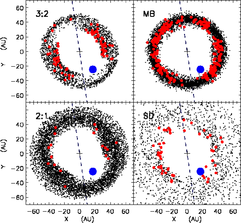
Figure 16: Black dots indicate the positions of all simulated particles relative to Neptune recorded at all times later than $t=3$ Gyrs. Red dots indicate the ecliptic coordinates of the observed multi-opposition KBOs, shown for July 1, 2000, which is the date by which half of the sample considered here had been discovered. The blue dot is Neptune’s position on this date, and the dashed line shows where the galactic plane penetrates the ecliptic $x$–$y$ plane. The particles and KBOs are sorted by their dynamical membership: bodies in or very near the 3:2 resonance (upper left), Main Belt (MB, upper right), 2:1 (lower left), and the so–called Scattered Disk Objects (SD, lower right) having perihelia $30<q<40$ AU and $a>48.4$ AU.

The Monte Carlo model of Section 6 replicates each Nbody survivor seen in Fig. 3 $10^{4}$ times by randomizing the particles’ mean anomalies, which results in a model Kuiper Belt having azimuthal symmetry. Thus the model implicitly assumes that the Kuiper Belt has this same symmetry. However one might question this assumption, since it is well known that a planet’s resonant perturbations can rearrange the longitudes of a small body population. For instance, particles at Neptune’s 3:2 tend to approach perihelion at longitudes that are $\sim 90^{\circ}$ away from the planet (Malhotra, 1995). This is illustrated in the upper left corner of Fig. 16, which shows the ecliptic coordinates of all simulated particles that are in or very near Neptune’s 3:2 resonance. This figure shows that Neptune tends to arrange the 3:2 bodies preferentially away from the Sun–Neptune line, causing regions that lead/trail Neptune by $\pm 90^{\circ}$ to be more densely populated, termed ‘sweet spots’ in Chiang & Jordan (2002). Figure 16 shows that resonant shepherding also occurs at Neptune’s 2:1, again similar to that seen in Chiang & Jordan (2002). Red dots indicate the positions of the multi–opposition KBOs considered here, which shows that KBOs in or near the 3:2 resonance tend to be discovered at longitudes that are roughly $\pm 90^{\circ}$ away from Neptune, as expected.

It is thus possible that Neptune’s rearrangement of the Belt might skew our estimate of the resonant populations. If, for example, KBO astronomers were preferentially surveying the Belt along longitudes that are $\pm 90^{\circ}$ away from Neptune, they would detect a rather high sky–plane number density of KBOs in the 3:2. If we then assumed that this 3:2 number density were uniform about the entire ecliptic, we would overestimate the total 3:2 population. Similarly, if astronomers systematically observed the Belt towards Neptune or $180^{\circ}$ away, we would underestimate the 3:2’s average sky–plane density and undercount its total population. But if astronomers surveyed all longitudes with equal frequency, then these competing effects—due to Neptune pushing KBOs away from certain longitudes and towards other longitudes—should wash out, resulting in an estimate of the 3:2 population that is approximately reliable.

The upper right part of Fig. 16 shows the ecliptic coordinates of the observed multi–opposition Main Belt KBOs. Since the Main Belt population is likely azimuthally symmetric, these red dots should be a good indicator of where astronomers are looking for KBOs. It is quite clear from this figure that these astronomers’ lines–of–sight are not distributed uniformly about the ecliptic. For instance, these KBO hunters tend to avoid the galactic plane, which passes through the ecliptic along the dashed line. The MB figure also shows that astronomers have avoided a narrow portion of the 3:2’s ‘sweet spot’ that leads Neptune by about $90^{\circ}$. But it is also quite clear that these same astronomers are not systematically staring at the 3:2’s sweet spots, nor are they systematically avoiding them. Consequently, our simple visual inspection of this KBO sample indicates that our estimate of the 3:2 population will not be significantly baised towards under or overcounting the 3:2 population, and that the 3:2 abundance reported in Section 11 is indeed representative. A similar conclusion is also drawn for the much sparser 2:1 population.

Of course, this treatment succeeds only if the Monte Carlo method of Section 6 does not alter the particles’ radial distribution as they have their mean anomalies randomized by the replication process. However it is straighforward to show that this is indeed the case. For instance, randomizing the mean anomalies of the 3:2 population seen Fig. 16 does not change their radial distribution in any significant way.

Table 1: Abundance and mass of KBOs having radii $50<R<1000$ km assuming density $\rho=1$ gm/cm³ and albedo $p=0.04$

dynamical class	site (AU)	population	mass (M⊕)
Centaurs	$a<a_{N}$	$<80$	$<4\times 10^{-5}$
Trojans	$a=a_{N}$	$<1.1\times 10^{3}$	$<5\times 10^{-4}$
3:2	$a=39.5$	$2.7\times 10^{3}$	$3.1\times 10^{-3}$
Main Belt	$40.1\leq a\leq 47.2$	$1.3\times 10^{5}$	0.059
2:1	$a=47.8$	$5.3\times 10^{3}$	$2.4\times 10^{-3}$
Scattered Disk	$50<a<150\ \&\ 28<q<40$	$2.5\times 10^{4}$	0.011

Figure 1: The planets’ semimajor axes $a_{j}$ versus time t, as well as a few of Neptune’s mean motion resonances that are effective at trapping particles.

Figure 2: A simulation of Neptune’s migration into a dynamically cold Kuiper Belt. The model Kuiper Belt is initially composed of $10^{4}$ massless particles having semimajor axes randomly distributed over $20<a<80$ AU with a surface number density that varies as $a^{-2}$. The particles initial eccentricities are Rayleigh distributed about a mean $\langle e\rangle=0.001$, and their initial inclinations (which are measured with respect to the system’s invariable plane) are similarly distributed over $\langle\sin i\rangle=\langle e\rangle/2$, while their other angular orbit elements are uniformly distributed over $2\pi$. The four giant planets’ orbits migrate according to the prescription described in Section 2, and the black dots shows the simulated Kuiper Belt endstate—the particles’ $e$’s and $i$’s versus $a$ at time $t=5\times 10^{8}$ years. The red dots are the ecliptic orbit elements of KBOs reported by the Minor Planet Center as having been observed for at least two oppositions. The yellow dots indicate Neptune’s orbit, and the vertical dashes show the locations of Neptune’s various $j+k:j$ mean–motion resonances. Orbits having perihelia $q=30$ and 40 AU are also indicate by the curves.

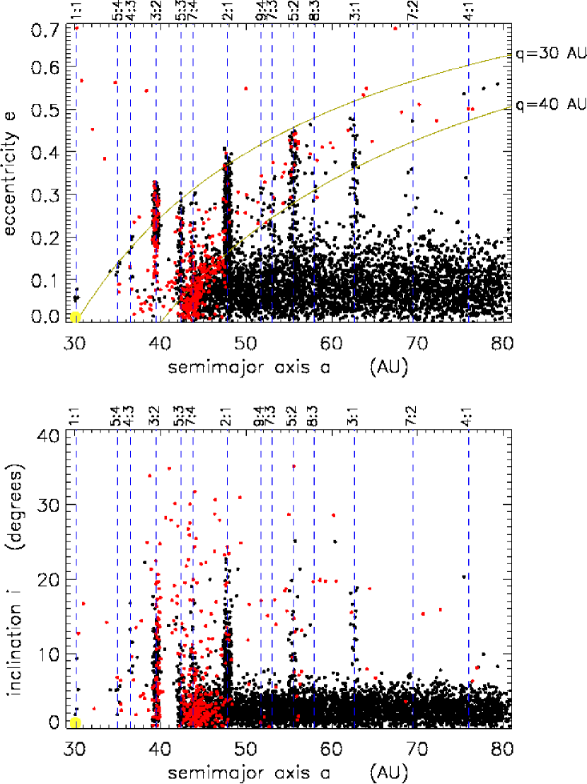
Figure 3: Neptune migrates into a dynamically hot disk of $N=10^{4}$ particles having initial $e$’s Rayleigh distributed about $\langle e\rangle=0.1$ and inclinations similarly distributed about $\langle\sin i\rangle=\langle e\rangle/2$, while all other initial orbits are distributed as in Fig. 2. This system is evolved for $t=4.5\times 10^{9}$ years.

Figure 6: The abundances of the Belt’s various dynamical populations are plotted over time $t$, with all populations normalized to the Main Belt (MB) population at time $t=4.5\times 10^{9}$ years, and counting only those particles having perihelia $q\leq 45$ AU. The resonant populations are counts of all particles having semimajor axes $\pm 0.6$ AU within exact resonance, while the MB curve gives the number of particles having semimajor axes $40.1\leq a\leq 47.2$ AU, excepting bodies in/near the 5:3 and 7:4 resonances. However the Scattered Disk (SD) curve is the number of particles having $a>49$ AU and perihelia $q<40$ AU that are not members of any of the indicated resonances (e.g., the 5:2 and 3:1), while Centaurs (C) are particles having $a<$ Neptune’s semimajor axis.

Figure 7: The dark–gray curve in the upper plot is the number of KBOs that have been observed (for two or more oppositions) orbiting in/near the 2:1 resonance having apparent magnitudes $m_{R}\pm\Delta m$ relative to the observed Main Belt (MB) population at $40.1\leq a\leq 47.2$ AU, while the lower dark–gray curve is the observed 3:2/MB ratio. Likewise, the light–gray curves are the 2:1/MB and 3:2/MB ratios for the simulation of Fig. 3, where these bodies’ sizes and magnitudes are assigned using the Monte Carlo method of Section 6 assuming $Q=4.4$ and $R_{min}=20$ km. All of these curves are smoothed over a magnitude–window having a half–width $\Delta m=0.5$, and the vertical half–width of the gray zones are one standard deviation assuming Poisson counting uncertainties. The observed curves end at $m_{R}\simeq 24.5$, which is the magnitude of the faintest multi–opposition KBO. The dashed curve is the simulated 3:2/MB ratio when the 3:2 population has a shallow size distribution with $Q=2.7$ and $R_{min}=4.3$ km, while the MB bodies have $Q=4.4$ and $R_{min}=20$ km.

Figure 13: The orbital history of the only simulated scattered object that inhabits the extended Scattered Disk (e.g., the large black dot in Fig. 12). The particle’s $a$, $e$, $q$ , $i$, and Tisserand parameter $T=a_{N}/a+2\sqrt{(a/a_{N})(1-e^{2})}\cos i$ are first plotted versus logarithmic time (left half of the Figure) and then linearly (right half). The dotted curves are Neptune’s semimajor axis $a_{N}$ and a few of its mean–motion resonances.

Figure 15: The smooth black curve is the Kuiper Belt’s observed ecliptic luminosity function $\Sigma(m_{R})$, obtained by integrating the differential luminosity function $d\Sigma(m_{R})/dm_{R}$ reported in Bernstein et al. (2004); note that it breaks to a shallower slope at magnitudes $m_{break}\simeq 24$. Dots give the simulation’s ecliptic luminosity function for particles in a truncated Kuiper Belt (see Section 11) having latitudes within $0.5^{\circ}$ of the ecliptic. Error bars are for Poisson counting statistics.

References

- Allen et al. (2001) Allen, R. L., Bernstein, G. M., & Malhotra, R. 2001, ApJ, 549, L241
- Altenhoff et al. (2004) Altenhoff, W. J., Bertoldi, F., Menten, K. M. 2004, A&A, 415, 771
- Bernstein et al. (2004) Bernstein, G. M., Trilling, D. E., Allen, R. L., Brown, M. E., Holman, M., & Malhotra, R. 2004, AJ, 128, 1364
- Borderies & Goldreich (1984) Borderies, N., & Goldreich, P. 1984, Celestial Mechanics, 32, 127
- Brouwer (1963) Brouwer, D. 1963, AJ, 68, 152
- Brown (2001) Brown, M. E. 2001, AJ, 121, 2804
- Brown et al. (2004) Brown, M. E., Trujillo, C., & Rabinowitz, D. 2004, Discovery of an inner Oort Cloud planetoid, ApJ, 617, 645
- Chambers (1999) Chambers, J. E. 1999, MNRAS, 304, 793
- Chiang & Jordan (2002) Chiang, E. I., & Jordan, A. B. 2002, AJ, 124, 3430
- Chiang & Lithwick (2005) Chiang, E. I., & Lithwick, Y. 2005, ApJ, in press
- Chiang et al. (2003) Chiang, E. I., Jordan, A. B., Millis, R. L., Buie, M. W., Wasserman, L. H., Elliot, J. L., Kern, S. D., Trilling, D. E., Meech, K. J., & Wagner, R. M. 2003, AJ, 126, 430
- Dermott et al. (1988) Dermott, S. F., Malhotra, R., & Murray, C. D. 1988, Icarus, 76, 295
- Dohnanyi (1969) Dohnanyi, J. W. 1969, J. Geophys. Res., 74, 2531
- Duncan et al. (1988) Duncan, M, Quinn, T., & Tremaine, S. 1988, ApJ, 328, L69
- Duncan & Levison (1997) Duncan, M. J., & Levison, H. F. 1997, Science, 276, 1670
- Duncan et al. (1995) Duncan, M. J., Levison, H. F., & Budd, S. M. 1995, AJ, 110, 3073
- Elliot et al. (2005) Elliot, J. L., Kern, S. D., Clancy, K. B., Gulbis, A. A. S., Millis, R. L., Buie, M. W., Wasserman, L. H., Chiang, E. I., Jordan, A. B., Trilling, D. E., &Meech, K. J. 2005, AJ, 129, 1117
- Fernández & Brunini (2000) Fernández, J. A., & Brunini, A. 2000, Icarus, 145, 580
- Fernandez & Ip (1984) Fernandez, J. A., & Ip, W.-H. 1984, Icarus, 58, 109
- Franklin et al. (2004) Franklin, F. A., Lewis, N. K., Soper, P. R., & Holman, M. J. 2004, AJ, 128, 1391
- Gladman et al. (2002) Gladman, B., Holman, M., Grav, T., Kavelaars, J., Nicholson, P., Aksnes, K., & Petit, J.-M. 2002, Icarus, 157, 269
- Gladman et al. (1998) Gladman, B., Kavelaars, J. J., Nicholson, P. D., Loredo, T. J., & Burns, J. A. 1998, AJ, 116, 2042
- Gomes (1997) Gomes, R. S. 1997, AJ, 114, 2166
- Gomes (2003) —. 2003, Icarus, 161, 404
- Gomes et al. (2004) Gomes, R. S., Morbidelli, A., & Levison, H. F. 2004, Icarus, 170, 492
- Grundy et al. (2005) Grundy, W. M., Noll, K. S., & Stephens, D. C. 2005, submitted to Icarus
- Hahn & Malhotra (1999) Hahn, J. M., & Malhotra, R. 1999, AJ, 117, 3041
- Hahn & Ward (1995) Hahn, J. M., & Ward, W. R. 1995, in Lunar and Planetary Institute Conference Abstracts, 541
- Hahn & Ward (2002) Hahn, J. M., & Ward, W. R. 2002, in Lunar and Planetary Institute Conference Abstracts, 1930–+
- Holman & Wisdom (1993) Holman, M. J., & Wisdom, J. 1993, AJ, 105, 1987
- Ida et al. (2000) Ida, S., Larwood, J., & Burkert, A. 2000, ApJ, 528, 351
- Irwin et al. (1995) Irwin, M., Tremaine, S., & Zytkow, A. N. 1995, AJ, 110, 3082
- Ivezić et al. (2001) Ivezić, Ž., Tabachnik, S., Rafikov, R., Lupton, R. H., Quinn, T., Hammergren, M., Eyer, L., Chu, J., Armstrong, J. C., Fan, X., Finlator, K., Geballe, T. R., Gunn, J. E., Hennessy, G. S., Knapp, G. R., Leggett, S. K., Munn, J. A., Pier, J. R., Rockosi, C. M., Schneider, D. P., Strauss, M. A., Yanny, B., Brinkmann, J., Csabai, I., Hindsley, R. B., Kent, S., Lamb, D. Q., Margon, B., McKay, T. A., Smith, J. A., Waddel, P., York, D. G., & the SDSS Collaboration. 2001, AJ, 122, 2749
- Jewitt & Luu (1995) Jewitt, D. C., & Luu, J. X. 1995, AJ, 109, 1867
- Kenyon & Luu (1999) Kenyon, S. J., & Luu, J. X. 1999, AJ, 118, 1101
- Kortenkamp et al. (2004) Kortenkamp, S. J., Malhotra, R., & Michtchenko, T. 2004, Icarus, 167, 347
- Levison & Duncan (1997) Levison, H. F., & Duncan, M. J. 1997, Icarus, 127, 13
- Levison & Duncan (2000) Levison, H. F. & Duncan, M. J. 2000, AJ, 120, 2117
- Levison & Stern (2001) Levison, H. F., & Stern, S. A. 2001, AJ, 121, 1730
- Levison & Morbidelli (2003) Levison, H. F., & Morbidelli, A. 2003, Nature, 426, 419
- Liou & Malhotra (1997) Liou, J. C., & Malhotra, R. 1997, Science, 275, 375
- Malhotra (1993a) Malhotra, R. 1993a, Icarus, 106, 264
- Malhotra (1993b) —. 1993b, Nature, 365, 819
- Malhotra (1995) —. 1995, AJ, 110, 420
- Malhotra (1996) —. 1996, AJ, 111, 504
- Malhotra & Williams (1997) Malhotra, R., & Williams, J. G. 1997, Pluto’s Heliocentric Orbit (Pluto and Charon), 127–+
- Malyshkin & Tremaine (1999) Malyshkin, L., & Tremaine, S. 1999, Icarus, 141, 341
- Morbidelli et al. (2002) Morbidelli, A., Jacob, C., & Petit, J.-M. 2002, Icarus, 157, 241
- Morbidelli & Levison (2004) Morbidelli, A., & Levison, H. F. 2004, AJ, in press
- Murray & Dermott (1999) Murray, C. D., & Dermott, S. F. 1999, Solar system dynamics (Solar system dynamics by Murray, C. D., 1999)
- Nagasawa & Ida (2000) Nagasawa, M., & Ida, S. 2000, AJ, 120, 3311
- Nesvorný & Dones (2002) Nesvorný, D., & Dones, L. 2002, Icarus, 160, 271
- Pittich & Rickman (1994) Pittich, E. M. & Rickman, H. 1994, A&A, 281, 579
- Rauch & Holman (1999) Rauch, K. P., & Holman, M. 1999, AJ, 117, 1087
- Sheppard et al. (2000) Sheppard, S. S., Jewitt, D. C., Trujillo, C. A., Brown, M. J. I., & Ashley, M. C. B. 2000, AJ, 120, 2687
- Sheppard et al. (2005) Sheppard, S. S., Trujillo, C., Jewitt, D. C., & Marsden, B. G., 2005, MPEC 2005-H21
- Stern & Campins (1996) Stern, A., & Campins, H. 1996, Nature, 382, 507
- Stern (1996) Stern, S. A. 1996, AJ, 112, 1203
- Stuart & Binzel (2004) Stuart, J. S., & Binzel, R. P. 2004, Icarus, 170, 295
- Tanga et al. (1999) Tanga, P., Cellino, A., Michel, P., Zappalà, V., Paolicchi, P., & dell’Oro, A. 1999, Icarus, 141, 65
- Thommes et al. (1999) Thommes, E. W., Duncan, M. J., & Levison, H. F. 1999, Nature, 402, 635
- Thommes et al. (2002) —. 2002, AJ, 123, 2862
- Tiscareno & Malhotra (2003) Tiscareno, M. S., & Malhotra, R. 2003, AJ, 126, 3122
- Tiscareno & Malhotra (2004) —. 2004, Chaotic Diffusion of Resonant Kuiper Belt Objects, submitted to AJ
- Trujillo & Brown (2001) Trujillo, C. A., & Brown, M. E. 2001, ApJ, 554, L95
- Trujillo et al. (2001) Trujillo, C. A., Jewitt, D. C., & Luu, J. X. 2001, AJ, 122, 457
- Tsiganis et al. (2005) Tsiganis, K., Gomes, R., Morbidelli, A. Levison, & H. F. 2005, Nature, in press.
- Ward (1981) Ward, W. R. 1981, Icarus, 47, 234
- Yu & Tremaine (1999) Yu, Q., & Tremaine, S. 1999, AJ, 118, 1873
- Zhou et al. (2002) Zhou, L., Sun, Y., Zhou, J., Zheng, J., & Valtonen, M. 2002, MNRAS, 336, 520