Taylor-Couette flow: MRI, SHI and SRI

Abstract

The linear stability theory of Taylor-Couette flows (unbounded in $z$) is described including magnetic fields, Hall effect or a density stratification in order to prepare laboratory experiments to probe the stability of differential rotation in astrophysics. If an axial field is present then the magnetorotational instability (MRI) is investigated also for small magnetic Prandtl numbers. For rotating outer cylinder beyond the Rayleigh line characteristic minima are found for magnetic Reynolds number of the order of 10 and for Lundquist numbers of order 1. The inclusion of extra toroidal current-free fields leads to new oscillating solutions with rather low Reynolds numbers and Hartmann numbers. The Hall effect establishes an unexpected ‘shear-Hall instability’ (SHI) where shear and magnetic field have opposite signs. In this case even rotation laws increasing outwards may become unstable. Recently global solutions have been found for the Taylor-Couette flows with density stratified in axial directions (‘stratorotational instability’, SRI). They exist beyond the Rayleigh line for Froude numbers of moderate order but also not for too flat rotation laws with $\hat{\eta}^{2}<\hat{\mu}<\hat{\eta}$.

1 Introduction

The rotation law in the infinite (in axial direction) Taylor-Couette flow is ${\Omega}(R)=a+b/{R^{2}},$ where $a$ and $b$ are related to the angular velocities ${\Omega}_{\rm in}$ and ${\Omega}_{\rm out}$ of the inner and the outer cylinders. The rotation laws with $a=0$ are called as located at the Rayleigh line. With $R_{\rm in}$ and $R_{\rm out}$ as the radii of the cylinders the parameters $\hat{\mu}={{\Omega}_{\rm out}}/{{\Omega}_{\rm in}}$ and $\hat{\eta}={R_{\rm in}}/{R_{\rm out}}$ of the flow are defined. According to the Rayleigh criterion the ideal flow is hydrodynamically stable when the specific angular momentum increases outwards, i.e. $\hat{\mu}>\hat{\eta}^{2}$ or $a>0$. The viscosity, however, stabilizes the flow so that it becomes unstable only if the inner cylinder rotates sufficiently fast.

           

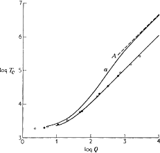
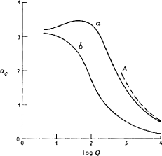
Figure 1: Early results for small gap and small Pm (Chandrasekhar 1961). Left: The influence of the magnetic field (Q here the Hartmann number) on the critical Taylor number. Magnetic fields suppress the instability. Right: The same for the wave number. The magnetic field elongates the Taylor vortices in the vertical direction. Boundary conditions: (a) conducting walls, (b) insulating walls.

If the fluid is electrically conducting and an axial magnetic field is applied then after the old results the critical Reynolds number (for the inner rotating cylinder) grows with growing magnetic field. Figure 1 shows the theoretical results of Chandrasekhar (1961) for narrow gaps and very small magnetic Prandtl numbers, ${\rm Pm}=\nu/\eta$, together with the experimental data for Mercury of Donnelly & Ozima (1960). Theory and observations are in nearly perfect agreement with no indication of any magnetic-induced instability. The magnetic Prandtl number under laboratory conditions is really very small ($10^{-5}$ for liquid sodium).

Within the small-gap approximation but with free Pm Kurzweg (1963) found that for weak magnetic fields and sufficiently large magnetic Prandtl number the critical Taylor number becomes smaller than in the hydrodynamic case (Fig. 2). If the field is not too strong it can basically play a destabilizing role.

Velikhov (1959) originally discovered this magnetic shear-flow instability which is now called ‘magnetorotational instability’ (MRI). He found that for the ideal hydromagnetic Taylor-Couette flow the Rayleigh criterion for stability changes to $\hat{\mu}>1,$ i.e. only flows with superrotation are still stable. He found a growth rate along the Rayleigh line (i.e. $a=0$) of $2{\Omega}_{\rm in}\hat{\eta}$ and a critical wave number of

$$k\leq 2\hat{\eta}\frac{{\Omega}_{\rm in}}{V_{\rm A}},$$ (1)

with $V_{\rm A}$ the Alfvén velocity of the given axial field. Only if $V_{\rm A}$ is smaller than the shear $-R^{2}{\rm d}{\Omega}/{\rm d}R$ the instability works which, therefore, is a weak-field instability.

The hydrodynamic Taylor-Couette flow is stable if its angular momentum increases with radius, but the hydromagnetic Taylor-Couette flow is only stable if the angular velocity itself increases with radius. This remains true also for nonideal fluids. The MRI reduces the critical Reynolds number for weak magnetic field strengths for hydrodynamically unstable flow and it destabilizes the otherwise hydrodynamically stable flow for $\hat{\eta}^{2}<\hat{\mu}<1.$ The MRI exists, however, in hydrodynamically unstable situations ($\hat{\mu}<\hat{\eta}^{2}$) only if Pm is not very small (Fig. 2).

As we shall demonstrate the magnetic Reynolds number

$$\rm Rm=Re\ Pm$$ (2)

controls the instability. Because of the high value of $\eta$ for liquid metals (exceeding 1000 cm²/s), it is not easy to reach magnetic Reynolds numbers of the required order of $1\dots 10$. This is the basic reason why the MRI has not yet been observed experimentally in the laboratory.

Figure 2: Critical Taylor number as a function of the magnetic Prandtl number for strong and weak magnetic fields within the small-gap approximation. For weak fields and large magnetic Prandtl numbers the system is subcritical. For $B_{0}=0$ (or, what is the same, for ${\rm Pm}=0$) is Ta${}_{\rm crit}=1750$. (Kurzweg (1963).

2 Magnetorotational instability (MRI)

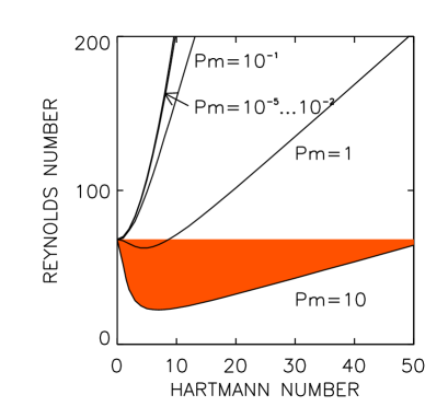
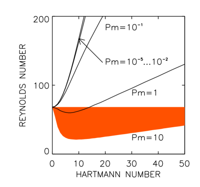
Figure 3: Bifurcation diagram for axisymmetric modes with resting outer cylinder of conducting material (left) and vacuum (right). Shaded areas denote subcritical excitation by the axial magnetic field. $\hat{\eta}=0.5$. From Rüdiger, Schultz & Shalybkov (2003).

The Reynolds number is usually defined as ${\rm Re}=R_{\rm in}(R_{\rm out}-R_{\rm in})\Omega_{\rm in}/\nu$. The amplitude of the external magnetic field $B_{0}$ is expressed with the Hartmann number ${\rm Ha}=B_{0}\sqrt{R_{\rm in}(R_{\rm out}-R_{\rm in})/(\mu_{0}\rho\nu\eta)}$. The values of the Reynolds numbers above which the flow becomes unstable depend on the vertical wave number. They have a minimum at some wave number for fixed other parameters. This minimum value is called the critical Reynolds number. Figure 3 shows the neutral stability for axisymmetric modes for containers with both conducting and insulating walls with resting outer cylinder and for fluids of various magnetic Prandtl number. ${\rm Re}=68$ is the classical hydrodynamic solution for resting outer cylinder and $\hat{\eta}=0.5$. There is a strong difference of the bifurcation lines for ${\rm Pm}\lower 1.72218pt\hbox{$\;\buildrel>\over{\scriptstyle\sim}\;$}1$ (high conductivity) and ${\rm Pm}<1$ (low conductivity). For fluids with low electrical conductivity the magnetic field only suppresses the instability so that all the critical Reynolds numbers strongly exceed the value 68.

For small magnetic Prandtl number the stability lines hardly differ. The opposite is true for ${\rm Pm}\lower 1.72218pt\hbox{$\;\buildrel>\over{\scriptstyle\sim}\;$}1$. In Fig. 3 the resulting critical Reynolds numbers Re are smaller than 68. The magnetic fields with small Hartmann numbers support the instability rather than to suppress it. This effect becomes more effective for increasing Pm but it vanishes for stronger magnetic fields. The MRI only exists for weak magnetic fields and high enough electrical conductivity and/or microscopic viscosity.

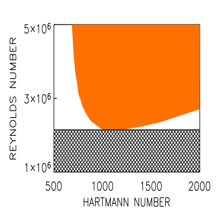
Figure 4: Marginal stability lines for axisymmetric modes in containers with rotating outer cylinder of conducting material for $\rm Pm=1$ ( left) and $\rm Pm=10^{-5}$ (right). $\hat{\eta}=0.5,\hat{\mu}=0.33$. The instability domain is colored by grey and fluids in the cross-hatched area are always stable.

Now the outer cylinder may rotate so fast that the rotation law no longer fulfills the Rayleigh criterion and a solution for ${\rm Ha}=0$ does not exist. The nonmagnetic eigenvalue along the vertical axis moves to infinity but a minimum remains. Figure 4 presents the results for $\rm Pm=1$ and $\rm Pm=10^{-5}$. There are always minima of Re for certain Hartmann numbers (Rüdiger & Shalybkov 2002). The minima and the critical Hartmann numbers increase for decreasing magnetic Prandtl numbers. For $\hat{\eta}=0.5$ and $\hat{\mu}=0.33$ the critical Reynolds numbers together with the critical Hartmann numbers are plotted in Fig. 5. Table 1 gives the exact coordinates of the absolute minima for experiments with rotating outer cylinder and for $\rm Pm=10^{-5}$. They are characterized by magnetic Reynolds numbers of order 10, very similar to the values of the existing dynamo experiments.

Table 1: Coordinates of the absolute minima in Fig. 4 for rotating outer cylinder with $\hat{\mu}=0.33$, $\hat{\eta}=0.5$ and $\rm Pm=10^{-5}$ .

	insulating walls	conducting walls
Reynolds number	$1.42\cdot 10^{6}$	$2.13\cdot 10^{6}$
mag. Reynolds number	14	21
Hartmann number	$1400$	$1100$
Lundquist number	4.42	3.47

A container with an outer radius of 22 cm (and an inner radius of 11 cm) filled with liquid sodium requires a rotation of about 19 Hz in order to find the MRI. The required magnetic field is about 1400 Gauss.

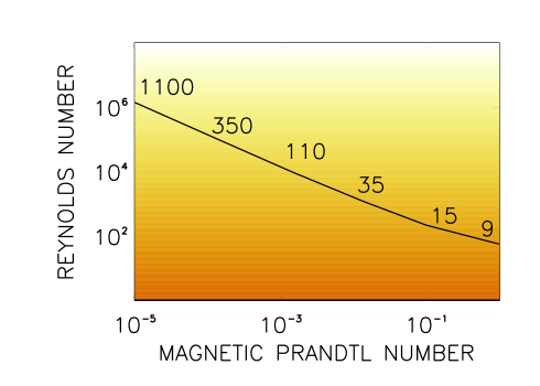
Figure 5: The critical Reynolds numbers vs. magnetic Prandtl numbers marked with those Hartmann numbers where the Reynolds number is minimum. $\hat{\eta}=0.5$, $\hat{\mu}=0.33$.

The results for containers with conducting walls are also given in Table 1. The minimal Reynolds numbers are higher than for insulating cylinder walls. The influence of the boundary conditions is thus not small.

There is a particular scaling for the special case of $a=0$, i.e. for $\hat{\mu}=\hat{\eta}^{2}$. One finds that the quantities $u_{R},u_{z},B_{R}$ and $B_{z}$ scale as ${\rm Pm}^{-1/2}$ while $u_{\phi},B_{\phi},k$ and Ha scale as ${\rm Pm}^{0}$. The Reynolds number for the axisymmetric modes scales as ${\rm Re}\propto{\rm Pm}^{-1/2}$ (Willis & Barenghi 2002). The scaling does not depend on the boundary conditions. However, for $a>0$ the much steeper scaling ${\rm Re}\propto{\rm Pm}^{-1}$ results , leading to the surprisingly simple relation

$${\rm Rm}\simeq{\rm const.}$$ (3)

for the magnetic Reynolds number Rm (Fig. 5). For the Lundquist number ${\rm S}={\rm Ha}\sqrt{{\rm Pm}}$ of the characteristic minima we find

$${\rm S}\simeq{\rm const.}$$ (4)

For small magnetic Prandtl numbers the exact value of the microscopic viscosity is thus not relevant for the instability. In consequence, the corresponding Reynolds numbers for the MRI seem to differ by 2 orders of magnitude, i.e. 10⁴ and 10⁶ at and shortly beyond the Rayleigh line. Figure 6 shows the behavior close to $\hat{\mu}=\hat{\eta}^{2}$. There is a vertical jump within an extremely small interval of $\hat{\mu}$. This sharp transition does not exist for ${\rm Pm}=1$; it only exists for very small values of Pm. Even the smallest deviation from the condition $\hat{\mu}=\hat{\eta}^{2}$ would drastically change the excitation condition.

Figure 6: Critical Reynolds numbers for the Taylor-Couette flow vs. $\hat{\mu}$ for $\hat{\eta}=0.27$ and ${\rm Pm}=1$ (left) and ${\rm Pm}=10^{-5}$ (right). From all $\hat{\eta}$, $\hat{\eta}=0.27$ yields the lowest minimum. The curve for the hydrodynamic instability (${\rm Ha}=0$) is dashed and the hydromagnetic curve (${\rm Ha}>0$) is solid. The dotted lines denote the location of $a=0$.

For $\hat{\eta}\simeq 0.5$ the Velikhov condition (1) can also be written as $kR_{\rm in}\simeq{\rm Rm/S}$. The vertical extension $\delta z$ of a Taylor vortex is given by

$$\frac{\delta z}{R_{\rm out}-R_{\rm in}}\simeq\frac{\pi}{k}\sqrt{\frac{\hat{\eta}}{1-\hat{\eta}}}.$$ (5)

The dimensionless vertical wave numbers $k$ associated with the critical Reynolds numbers are given in Fig. 7. For hydrodynamically unstable flows we have $\delta z\simeq R_{\rm out}-R_{\rm in}$ for small magnetic fields (${\rm Ha}\simeq 0$). The cell therefore has the same vertical extent as it has in radius.

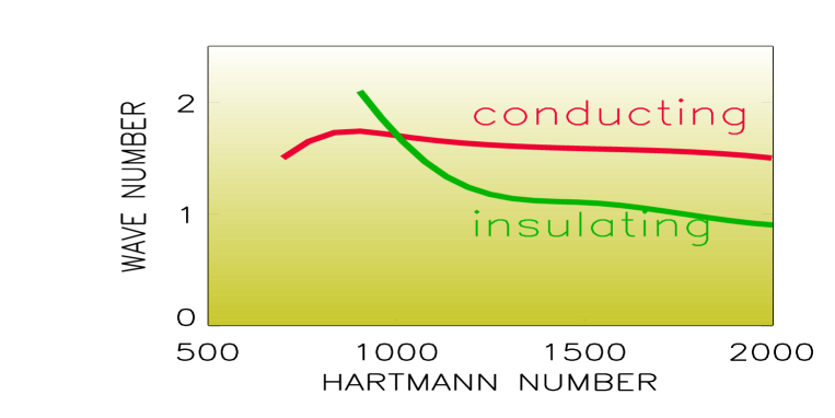
Figure 7: Wave numbers for which the Reynolds number is minimum for conducting walls and insulating walls. $\hat{\eta}=0.5$, $\hat{\mu}=0.33$, ${\rm Pm}=10^{-5}$. Note how exact the Velikhov condition (1) is fulfilled. From Rüdiger & Shalybkov (2002).

The magnetic fields deforms the Taylor vortices. The deformation consists in a elongation of the cell in the vertical direction. The wave number is thus expected to become smaller and smaller for increasing magnetic field. This is indeed true for ${\rm Pm}\simeq 1$, but for smaller Pm the situation is more complicated.

The cell size is minimum for the critical Reynolds number for all calculated examples of hydrodynamically stable flows with a conducting boundary. This is not true, however, for containers with insulating walls, for which the cell size grows with increasing magnetic field. For experiments with the critical Reynolds numbers the vertical cell size is generally 2–3 times larger than the radial one. The smaller the magnetic Prandtl number the longer are the cells in the vertical direction. The influence of boundary conditions on the cell size disappears for sufficiently wide gaps.

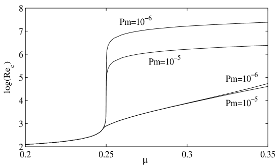
Figure 8: Critical Reynolds numbers for marginal stability of axisymmetric modes in containers ($\hat{\eta}=0.5$) with purely axial magnetic field (upper curves) and with extra (current-free) toroidal field (lower curves) for $\rm Pm=10^{-5}$ and $\rm Pm=10^{-6}$ as a function of $\hat{\mu}$. Note the extremely weak Prandtl number dependence of the lower curves and the strong reduction of the critical Reynolds numbers. From Hollerbach & Rüdiger (2005).

The given solutions of marginal stability of axisymmetric modes are stationary. One could ask for the character of the solutions if an extra toroidal magnetic field is applied (Hollerbach & Rüdiger 2005). We know that current-free toroidal fields alone do not change the stability of Taylor-Couette flow (Velikhov 1959). If axial fields and current-free toroidal fields of the same order exist in the container, however, completely new solutions appear and they are oscillating (Fig. 8). The real parts of the eigenfrequencies are positive so that stationary modes do not longer exist. The Reynolds number of the flow and the Hartmann number of the axial field which are necessary to induce the MRI instability are strongly reduced by the toroidal field. In Table 2 characteristic numbers from numerical experiments with small magnetic Prandtl number and for $\hat{\mu}=0.3$ are given.

Table 2: Characteristic values for $\hat{\eta}=0.5$, $\hat{\mu}=0.3$, $\rm Pm=10^{-5}$. $\beta$ describes the amplitude ratio of the toroidal and the axial magnetic field.

$\beta$	Re	Ha	$k$	$\Re(\omega)$
0	$1.6\cdot 10^{6}$	850	1.7	0
1	$5.8\cdot 10^{5}$	383	0.47	0.04

3 Shear-Hall instability (SHI)

In the presence of the Hall effect there is even the possibility that differential rotation with $\Omega$ increasing outwards (i.e. $\partial\Omega/\partial R>0$) becomes unstable. The Hall effect destabilizes flows with $\hat{\mu}>1$ for which so far no other instability is known. The dispersion relation derived from the equation system with an induction equation including Hall effect leads to the instability condition ${\rm Rb}\ \partial\Omega/\partial R<0$ with Rb as the ratio of the Ohmic time scale and the Hall time scale. It linearly depends on the electrical conductivity and the magnetic field (see Rüdiger & Hollerbach 2004). For magnetic fields parallel to the rotation axis it might be positive and v.v. The result depends on the sign of the Hall resistivity; here the positive Hall resistivity is used.

Figure 9: The shear-Hall instability. Only the induction equation is solved for Taylor-Couette flows under the presence of the Hall effect. Left: magnetic field positive, shear negative. Right: magnetic field negative, shear positive. The lines of marginal instability are labeled with the actual value of $\hat{\mu}$.

Figure 9 illustrates the instability for a container with again $\hat{\eta}=0.5$. The flow with $\hat{\mu}<1$ is unstable for positive Rb. Flows with $\hat{\mu}>1$ are unstable for negative Rb, i.e. if angular velocity and magnetic field have opposite directions. The fact that the Hall effect destabilizes flows with the angular velocity increasing outwards was first described by Balbus and Terquem (2001).

Figure 9 may only serve as an illustration. In particular for $\hat{\mu}<1$ the situation is more complicated as simultaneously the MRI is active. One finds more details in the original paper of Rüdiger & Shalybkov (2004) about the overall impact of the Hall effect on the Taylor-Couette flow. That the sign of the magnetic field has such an important influence on stability or instability of flows (e.g. Kepler flows) must have important consequences for astrophysical applications.

Figure 10: The lines of marginal instability for $\hat{\mu}=2$ with axisymmetric ($m=0$, solid line) and nonaxisymmetric ($m=1$, dotted line) modes. Left: conducting walls, note the crossover of both lines. Right: insulating walls, no crossovers. Here $\rm Ha=Rb$.

It is also important to know the nonaxisymmetric modes. After the Cowling theorem only nonaxisymmetric modes can be maintained by a dynamo process. We have discussed the appearance of nonaxisymmetric modes for the magnetic Taylor-Couette flow with negative shear (Shalybkov, Rüdiger & Schultz 2002). The common result was that the lines of marginal stability for $m=0$ and $m=1$ have a very different behavior for different electrical boundary conditions. One finds crossovers of the stability lines for containers with conducting cylinder walls, and one never finds crossovers for containers with vacuum boundary conditions. The same happens for the Hall instability for magnetic Taylor-Couette flows with $\hat{\mu}>1$. In Fig. 10 the lines for both axisymmetric and nonaxisymmetric modes are given for conducting boundary conditions and for vacuum boundary conditions. Indeed, a crossover of the lines only exists for conducting cylinder walls. As usual, in the minimum the $m=0$ mode dominates but for stronger magnetic fields the mode with $m=1$ dominates.

4 STRATOROTATIONAL INSTABILITY (SRI)

The hydrodynamic Taylor-Couette flow stability is now discussed under the presence of vertical density stratifications. Taylor-Couette flows with a stable axial density stratification were often studied with the conclusion that a stable stratification stabilizes the flow. Withjack & Chen (1974), however, reported new experiments with the Rayleigh line at $\hat{\mu}=0.04$. For a slight negative density gradient disturbances of spiral form were observed for $\hat{\mu}=0.073$, i.e. clearly beyond the Rayleigh line. Recently, Yavneh, McWilliams & Molemaker (2001) find that the sufficient condition for stability against nonaxisymmetric disturbances is the same as the condition for MRI. Their numerical results demonstrated that certain instabilities exist also for finite viscosity.

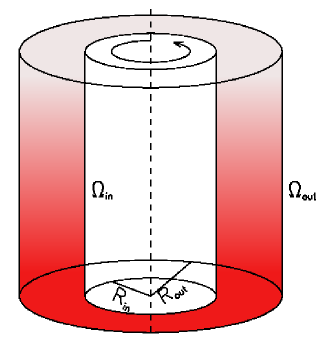
Figure 11: Taylor-Couette flow geometry with axial density stratification

One has to look for the basic state with prescribed velocity profile and given density vertical stratification $\rho=\rho(z)$. The initial system then can only exist if

$$R\Omega^{2}\frac{\partial\rho}{\partial z}+g\frac{\partial\rho}{\partial R}=0.$$ (6)

is fulfilled. Under the centrifugal force the purely vertical stratification at the beginning transforms to a mixed vertical and radial stratification. This behavior strongly complicates the problem.

In real experiments the initial vertical stratification is so small that $R^{2}\Omega\ll g$. Then after (6) the radial stratification is also small. Let us, therefore, consider the ‘small-stratification case’ with $\rho=\rho_{0}+\rho_{1}(R,z)$ with $\rho_{1}\ll\rho_{0}$, where $\rho_{0}$ is the uniform background density and condition (6) is fulfilled at zero order. If only the terms of the zero order are considered then the system takes the Boussinesq form. $N$ is the vertical Brunt-Väisälä frequency $N^{2}=-(g/\rho_{0})\partial\rho_{1}/\partial z$ and ${\rm Fr}=\Omega_{\rm in}/N$ is the Froude number.

Here we suppose $\partial\rho_{1}/\partial z={\rm{const}}$ so that the coefficients of the system only depend on the radial coordinate and a normal mode expansion $~{}{\rm{exp}}({\rm{i}}(m\phi+kz+\omega t))$ is possible. As usual, only those wave numbers are considered which belong to the smallest Reynolds numbers. We have also checked the existence of the transition from stable to unstable state for some arbitrary points.

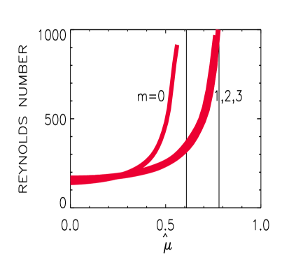
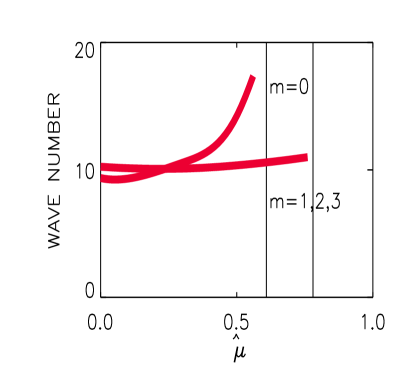
Figure 12: Left: The marginal stability lines for $m\geq 0$. The vertical lines mark the Rayleigh line $\hat{\mu}=\hat{\eta}^{2}$ (left) and the outer limit line $\hat{\mu}=\hat{\eta}$ (right). Right: The vertical wave numbers are very large. $\hat{\eta}=0.78$, $\rm Fr=0.5$. From Shalybkov & Rüdiger (2005).

The dependence of the critical Reynolds numbers on $\hat{\mu}$ is given in Fig. 12 (left). The already known marginal stability line for $m=0$ and also the new lines for $m>0$ are plotted. Note that the critical Reynolds numbers are remarkable small. The axisymmetric disturbances are unstable only for $\hat{\mu}<\hat{\eta}^{2}$ in accordance to the Rayleigh condition. The new nonaxisymmetric disturbances are also unstable in the interval $\hat{\eta}^{2}<\hat{\mu}<\hat{\eta}$. The existence of the outer limit $\hat{\mu}=\hat{\eta}$ is a new and surprising finding. Even more flat rotation laws with $\hat{\mu}>\hat{\eta}$ are still stable (Shalybkov & Rüdiger 2005).

For $m>0$ the vertical wave number only slightly depends on $m$ (Fig. 12, right). The wave numbers are so large that the cells are flat in the axial direction. The vertical wave number does hardly depend on $\hat{\mu}$.

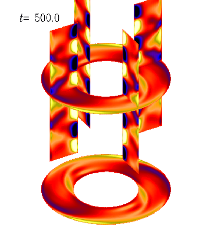
Figure 13: The global stratorotational instability for $\hat{\mu}=0.3$, $\rm Fr=0.32$, $\rm Re=500$ and $\rm Pr=10$. Note the $m=2$ azimuthal structure. From Brandenburg & Rüdiger (2005).

By Brandenburg & Rüdiger (2005) the global problem is treated in Cartesian geometry with the nonlinear Pencil code. For a Reynolds number of about 500 a resolution of 128³ mesh points was sufficient. Again $\hat{\eta}=0.5$. As expected, no instability is found for $\hat{\mu}=0.6$. For smaller values ( $\hat{\mu}=0.2$) the flow is Rayleigh unstable. For $\hat{\mu}=0.3$ the flow is indeed stratorotationally unstable for nonaxisymmetric modes also in the nonlinear regime. The modes are saturated and they are azimuthally drifting. Cross sections of $u_{z}$ are shown in Fig. 13 for $\hat{\mu}=0.3$ and $\rm Fr=0.32$. Note that there are 4 eddies in $z$-direction. The growth rate, however, with $0.01\Omega_{\rm in}$ proves to be rather small (see also Dubrulle et al. 2005).

5 References

Balbus, S.A., Terquem, C., ApJ, 552, 235 (2002).
Brandenburg, A., Rüdiger, Astronomy & Astrophysics, in prep. (2005).
Chandrasekhar, S., Hydrodynamic & Hydromagnetic Stability, Oxford (1961).
Donnelly, R.J., Ozima, M., Phys. Rev. Lett., 4, 497 (1960).
Dubrulle, B., Marie, L., Normand, Ch. et al., Astronomy & Astrophysics, 429, 1 (2005).
Hollerbach, R., Rüdiger, G., Science, in preparation (2005).
Kurzweg, U.H., J. Fluid Mech., 17, 52 (1963).
Rüdiger, G., Shalybkov, D., Phys. Rev. E, 66, 016307 (2002).
Rüdiger, G., Schultz, M., Shalybkov, D., Phys. Rev. E, 67, 046312 (2003).
Rüdiger, G., Shalybkov, D., Phys. Rev. E, 69, 016303 (2004).
Rüdiger, G., Hollerbach, R., The magnetic universe, Wiley (2004).
Shalybkov, D., Rüdiger, G. Schultz, M., Astronomy & Astrophysics, 395, 339 (2005).
Shalybkov, D., Rüdiger, G., Astronomy & Astrophysics, subm. (2005).
Velikhov, E.P., Sov. Phys. JETP, 9, 995 (1959).
Willis, A.P., Barenghi, C.F., Astronomy & Astrophysics, 393, 339 (2002).
Withjack, E.M., Chen, C.F., J. Fluid Mech., 66, 725 (1974).
Yavneh, I., McWilliams, J.C., Molemaker, M.J., J. Fluid Mech., 448, 1 (2001).