Baryon oscillations

Abstract

The coupling of photons and baryons by Thomson scattering in the early universe imprints features in both the Cosmic Microwave Background (CMB) and matter power spectra. The former have been used to constrain a host of cosmological parameters, the latter have the potential to strongly constrain the expansion history of the universe and dark energy. Key to this program is the means to localize the primordial features in observations of galaxy spectra which necessarily involve galaxy bias, non-linear evolution and redshift space distortions. We present calculations, based on mock catalogues produced from particle-mesh simulations, which show the range of behaviors we might expect of galaxies in the real universe. We find that non-linearity, galaxy bias and redshift space distortions all introduce important modifications to the basic picture. Both the galaxy bias and the (isotropic) redshift space distortions lead to relatively smooth modulations in power on the scales of interest to baryon oscillations. The halo and galaxy power spectra exhibit low order structure beyond the acoustic oscillations over the range of scales of relevance. Fitting a cubic polynomial to the ratio of galaxy to dark matter power reduces any remaining structure in the range $0.03\leq k\leq 0.3\,h\,{\rm Mpc}^{-1}$ below the 2% level, which is close to the error in our calculations.

1 Introduction

Recently Eisenstein and collaborators SDSS , using data from the Sloan Digital Sky Survey, published evidence for features in the matter power spectrum on scales of $100\,$Mpc. These features, long predicted, hold the promise of another route to understanding the expansion history of the universe and the influence of dark energy.

It was realized very early GrandDad that a universe with non-negligible baryon fraction would result in significant features in the matter power spectrum due to the coupling of the baryons to (hot) photons in the early universe. When the universe was dense and highly ionized the baryons and photons were tightly coupled by Thomson scattering. During this phase the amplitude of baryon-photon perturbations cannot grow, but rather undergo harmonic motion with a slowly decaying amplitude. Slightly after recombination the baryons decouple from the radiation and the oscillations are frozen in – leading to subtle features in the total matter power spectrum analogous to the (fractionally much larger) features in the power spectrum of the cosmic microwave background (CMB) radiation. The first calculations to emphasize the oscillations in the context of hot big-bang CDM models were Early .

Figure 1: The rms fluctuations in the radiation and matter as a function of wavenumber, $k$. The structure in the CMB spectrum is familiar, in its $\ell$-space form, from the WMAP measurements WMAP . For the matter spectrum we have divided by $k$ to remove the overall trend and enhance the appearance of the oscillations. Note that the precise relationship between the oscillations in the CMB and in the mass is complex but the same physical processes affect both.

We show in Fig. 1 the matter and radiation power spectra, in $k$-space, for a $\Lambda$CDM model (see below). These spectra were computed by numerical evolution of the coupled Einstein, fluid and Boltzmann equations as described in Boltz ; SSWZ . A description of the physics leading to the oscillations can be found in EHSS or Appendix A of MeiWhiPea . While the precise relationship between the positions of the peaks in the radiation and matter power spectra is complex, the same physics underlies both and they share a common scale: the sound horizon

$$s=\int c_{s}(1+z)dt\simeq 147\pm 2\ {\rm Mpc}$$ (1)

where $c_{s}$ is the sound speed and the measured value is taken from WMAP . The peaks in the radiation spectrum occur roughly at $ks=n\pi$ for integer $n$, the peaks in the matter spectrum are almost out of phase.

It was pointed out in Refs. CooHuHutJof ; Eis03 that this scale could be used as a standard ruler to constrain the distance-redshift relation, the expansion of the universe and dark energy. Numerous authors Fisher have now observed that a high-$z$ galaxy survey covering upwards of several hundred square degrees could place interesting constraints on dark energy. Key to realizing this is the ability to accurately predict, from measurements of the CMB, the physical scale at which the oscillations appear in the power spectrum plus the means to localize those primordial features in observations of galaxy spectra which necessarily involve galaxy bias, non-linear evolution and redshift space distortions. The former problem seems well in hand SSWZ ; EisWhi . We make some preliminary investigations of the latter problem in this paper.

2 Fitting the extra physics

The real space, linear theory matter power spectrum can be computed with high accuracy SSWZ , however we measure the non-linear galaxy power spectrum in redshift space. Our understanding of the transformation between these two is improving rapidly, along with our ability to simulate the complex processes involved. Thus to some degree the effects of non-linearity, bias and redshift space distortions can be predicted. However, we would like to reduce our dependence on detailed theoretical calculations as much as possible. One possibility is to parameterize the additional effects and measure the parameters along with the sound horizon. This amounts to marginalizing over a range of models for the additional physics, inflating the error bars on the cosmological parameters but reducing sensitivity to improper modeling of non-linearity, bias or redshift space distortions. In general we would like to allow enough freedom in our fit to account for the effects while not degrading too severely our constraint on the peak locations. Improved theoretical modeling of non-linearity, bias and redshift space distortions translate into stronger priors on the “extra physics” parameters in this framework.

Figure 2: A slice, $10\,h^{-1}$Mpc thick, through the DM distribution in the higher resolution run at $z=1$. The greyscale is logarithmic in density with black being $>10^{2}\bar{\rho}$ and white being $<10^{-2}\bar{\rho}$.

Non-linearity, galaxy bias and redshift space distortions are all expected to be “simple” on large scales. Each has a characteristic scale associated with it. For non-linearity the scale is $k^{-1}_{\rm nl}\simeq 1-5\,h^{-1}$Mpc for $z\simeq 0.3-3$ (see §4). For redshift space distortions the scale is set by the velocity dispersion of the largest halos HaloRed . At $z\simeq 1$ we expect $\sigma\simeq 500\,{\rm km}{\rm s}^{-1}\sim 5\,h^{-1}$Mpc. Galaxy bias is expected to become simple on large scales SchWei and in halo-based models Halo the transition is set by the virial radius of the largest halo, $r_{0}\simeq 1\,h^{-1}$Mpc. Thus it makes sense to fit, for $k<0.1\,h{\rm Mpc}^{-1}$,

$$\Delta^{2}_{\rm obs}(k)=B^{2}(k)\Delta^{2}_{\rm dm}(k)+C(k)$$ (2)

with $\Delta^{2}_{\rm dm}(k)$ the dimensionless power spectrum,

$$\Delta^{2}(k)\equiv\frac{k^{3}P(k)}{2\pi^{2}}\quad{\rm with}\quad P(\vec{k})\equiv\left|\delta_{\vec{k}}\right|^{2}$$ (3)

of the mass, in real space, and $B(k)$ and $C(k)$ are polynomials in $k$. Within the halo model $B(k)$ describes the $2$-halo term while $C(k)$ describes the $1$-halo term Nikhil . Since we are not computing $B(k)$ and $C(k)$ from a halo model formalism, but merely exploring the relationship between $\Delta^{2}_{\rm obs}(k)$ and $\Delta^{2}_{\rm dm}(k)$, we will take a slightly simpler approach (see later) of absorbing $C(k)$ into a scale dependent bias, $b(k)$. We note that the authors of Ref. SeoEis05 make a different reduction by taking $B(k)=$constant and absorbing any scale-dependence into $C(k)$.

As an example of the above approach we could expand the corrections to our best fit theory in Hermite polynomials, $H_{n}$, which are bounded by $-1\leq H_{n}\leq 1$. Theoretical priors would then take the form of limits on the size of the correction coefficients, for example $c_{n}$ is a Gaussian of zero mean and dispersion $\sigma_{n}$ which parameterizes the residual uncertainty in our modeling. In this paper we make a preliminary investigation of the structure of these functions using numerical simulations.

3 Simulations

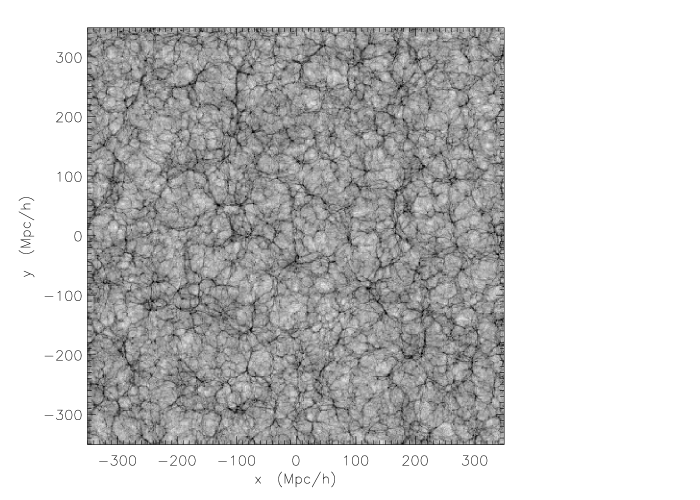
The basis for our calculations is a sequence of particle-mesh (PM) simulations of a $\Lambda$CDM cosmology ($\Omega_{M}=0.28=1-\Omega_{\Lambda}$, $\Omega_{B}\simeq 0.049$, $n=1$, $\sigma_{8}=0.9$ and $h=0.7$) in a periodic, cubical box of side $700\,h^{-1}$Mpc=$1\,$Gpc. The main simulation evolved $1024^{3}$ particles of mass $2.5\times 10^{10}\,h^{-1}M_{\odot}$ from $z=60$ to $z=0$ with a regular mesh of $2048^{3}$ points used to compute the forces. Outputs at both fixed time and along a light-“cone” were produced at $z=4$, 3, 2, 1.5, 1, 0.3 and 0 (see Fig. 2). To make the geometry easier for analysis we assumed the infinitely distant observer approximation in producing the light-cone outputs. The rays did not converge on the origin, but rather were all parallel to the $\hat{z}$-axis of the simulation box, respecting the periodic nature of the simulation. For some of our results on the rarer, more massive halos we used a series of 9 lower resolution ($512^{3}$) simulations with the same size box.

For the initial conditions we used the linear theory power spectrum from Fig. 1 and displaced particles from a “fuzzy” regular grid using the Zel’dovich approximation. For the main simulation we picked random phases, but for the amplitudes of the low-$k$ modes we chose an abnormally common set. The power spectrum at low-$k$ thus shows significantly less scatter than a Rayleigh distribution, making it easier to see the baryonic features. Moving to higher $k$, with more modes in the box, we gradually moved to a Rayleigh distribution so that the initial conditions properly sampled a Gaussian distribution. Since we are primarily interested in the effects of galaxy modeling, redshift space distortions and light-cone evolution the exact initial conditions are merely a convenience. For the smaller runs we chose unconstrained Gaussian initial conditions, since we can average over several realizations.

For each output we generate a catalog of halos using the Friends-of-Friends algorithm FoF with a linking length of $b=0.15$ in units of the mean inter-particle spacing. This procedure partitions the particles into equivalence classes, by linking together all particle pairs separated by less than a distance $b$. The groups correspond roughly to all particles above a density of $3/(2\pi b^{3})\simeq 140$ times the background density and we keep all groups with more than 20 particles.

Figure 3: The positions of halos hosting galaxies in a $10\,h^{-1}$Mpc slice through a $200\,h^{-1}$Mpc simulation of a $\Lambda$CDM model with a high force resolution code TreePM and the PM code used in this work. The simulations each evolved $256^{3}$ particles from the same initial conditions to $z=0$. The filled (red) squares are halos from the high-resolution run, the (blue) open circles those from the PM run.

Figure 4: The mass function of halos in the PM simulation at $z=3$, 1 and 0.3. The lines indicate the prediction of Ref. ST . The shortfall at low mass is due to the limited force resolution of the PM simulation.

The huge advantage of a PM simulation over one involving higher force resolution is its speed or low cost. The current simulations, plus all of the post-processing took only $\sim 10^{4}$ CPU hours on the IBM-SP Seaborg at NERSC — a few percent of the resources required for the Hubble volume HV or Millennium runs Millenium . It is easy to conceive of running large numbers of PM simulations of this size to explore parameter space or provide statistical samples – but is a PM simulation adequate?

We would like to follow a large number of particles to accurately evolve the modes in the quasi-linear regime, but the baryon oscillation scales are very large so don’t require a huge dynamic range. Indeed PM simulations on a 1990’s era mid-level desktop workstation were perfectly adequate to resolve the relevant gravitational physics and explore simple models of galaxy bias MeiWhiPea . Our main simulation resolves the relevant scales with hundreds of mesh cells in each dimension.

The issue of galaxy modeling is more subtle. Clearly our simulations are not correctly resolving the internal structure of dark matter halos hosting galaxies, and are completely unable to resolve sub-structure. This makes careful modeling of galaxy formation impossible. We shall take a different approach however. Rather than trying to model as accurately as possible the physics of galaxy formation, we shall try to get a feel for the range of possibilities afforded by models in which galaxies form in dark matter halos. If we are willing to make assumptions about the spatial and velocity distribution of galaxies in halos and their halo occupation distribution then we need only resolve the positions and masses of the hosting halos in the simulation in order to make realistic mock catalogs – an approach similar to that of Ref. PTHalos .

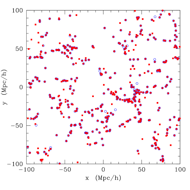
Fortunately the masses and positions of the halos are reasonably well modeled, as we show in Fig. 3. The figure shows the $x$ and $y$ positions of halos which would host galaxies in a thin slice through two simulations. Both simulations have the same initial conditions, one is run with a high force resolution code TreePM and one with the PM code. The overall agreement in positions and masses is very good, although there is a tendency for the PM simulation to merge some close halos that the higher resolution simulation resolves as discrete. A few of the halos seen in one simulation but not the other have their centers falling just outside of the thin slice in one run but inside in the other. The mass function of the simulation at $z=3$, 1 and 0.3 is shown in Fig. 4 compared to the fitting function of Ref. ST . There is a shortfall at lower masses and an excess at the very rare, high mass end – the excess appears to come from the initial conditions used, the shortfall at low mass comes from the finite force resolution. For halos in the most interesting range for us, few $\times 10^{12}$ – $10^{14}\,h^{-1}M_{\odot}$, the agreement is satisfactory. Based on these comparisons we believe that our simulations, while inappropriate to model small scale clustering, are adequate for our purposes.

$\log_{10}M_{\rm min}$	$\log_{10}M_{1}$	$\langle b\rangle$
12.8	13.0	2.4
12.6	13.5	2.0
12.5	14.0	1.8
12.5	14.5	1.8

Table 1: The HOD parameters, for the form of Eq. 4, we have used for some of our models at $z=1$. Masses are in units of $h^{-1}M_{\odot}$ and the number density for all models is $10^{-3}\,h^{3}\,{\rm Mpc}^{-3}$.

To make the mock galaxy samples we then take an output and choose a mean occupancy of halos: $N(M)\equiv\left\langle N_{\rm gal}(M_{\rm halo})\right\rangle$. Each halo either hosts a central galaxy or does not. For each halo we define a galaxy to live at the minimum of the halo potential, with the center of mass velocity, with probability $p={\rm max}[1,N(M)]$. Following Ref. KBWKGAP , if $N(M)>1$ the mean number of satellites, $N_{\rm sat}=N(M)-1$, is computed for the halo and a Poisson random number, $n_{\rm sat}$, drawn. Then $n_{\rm sat}$ dark matter particles, chosen at random but with weights depending on their radial distance from the potential minimum, are anointed as galaxies. Our fiducial model has equal weights – the satellite galaxies trace the dark matter. The galaxy velocity is taken to be $v_{\rm sat}=v_{\rm com}+A\left(v_{\rm part}-v_{\rm com}\right)$ where $v_{\rm part}$ is the particle velocity and $v_{\rm com}$ is the velocity of the halo center-of-mass and our fiducial model has $A=1$, i.e. $v_{\rm sat}=v_{\rm part}$. The result is a set of “galaxies” whose clustering properties can be computed. While the galaxy model is not prescriptive, or likely even close to “right”, it is physically well motivated, easy to adjust and leads to galaxy catalogs with non-linear, scale-dependent, stochastic (and in principle luminosity dependent) biasing, redshift space distortions and (later) light-cone effects.

Figure 5: The large-scale bias at $z=1$ as a function of number density, $\bar{n}$, and $M_{1}$ for a HOD of the form of Eq. 4. Contours are spaced in units of 0.25. The bias increases to lower left and $\langle b\rangle=2$ and 3 are shown as thick contours.

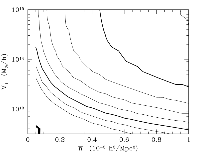
Even with the distribution of galaxies chosen there is still tremendous freedom in specifying $N(M)$. For this initial exploration we choose a very simple two-parameter form with

$$N(M)=\Theta(M-M_{\rm min})\ \frac{\left(M-M_{\rm min}\right)+M_{1}}{M_{1}}$$ (4)

where $\Theta(x)$ is the Heavyside step function. If we take $M_{1}\to\infty$ our catalog reduces to a catalog of halos more massive than $M_{\rm min}$. By holding $\bar{n}$ fixed we can specify a 1-parameter sequence of models with varying $M_{\rm min}$ or large-scale bias, $\langle b\rangle$, as shown in Fig. 5. A selection of models is given in Table 1.

For most of our results we will concentrate on the $z=1$ output. We still do not know what the best sample of galaxies is for detecting baryon oscillations at $z=1$. Since it is not our intention to model a particular strategy we will choose $\bar{n}=10^{-3}\,h^{3}\,{\rm Mpc}^{-3}$ – at the upper end of the range advocated by SeoEis03 for $z=1$. We find for samples with lower number density the shot-noise correction is very large and the sampling noise unacceptably high for our limited volume. A density of $10^{-4}$ is close to the observed number density of the SDSS luminous red galaxy (LRG) sample with $\langle z\rangle\simeq 0.3$. These galaxies have a large-scale bias of approximately two Zehavi . In our model, at this redshift, we can fit the number density and bias with $M_{\rm min}\simeq 3.3\times 10^{13}\,h^{-1}M_{\odot}$ and $M_{1}\simeq 10^{15}\,h^{-1}M_{\odot}$. If we imagine the HOD doesn’t evolve with redshift, and with $M_{1}$ this large, the LRGs are essentially the central galaxy population of halos above $M_{\rm min}$. Since this mass is quite large, and the halos quite rare, we use the lower resolution runs to study such massive halos. In future, with more simulations in hand, we could enlarge our study to other populations. Finally we note that for all of these number densities the contribution to the power spectrum from shot-noise, assuming it is Poisson, is as large as the signal on scales of $k\simeq 0.1\,h{\rm Mpc}^{-1}$. This is no accident – in the Gauss-Poisson limit the optimal survey strategy for constraining the power spectrum is to balance the cosmic variance and shot-noise power SparseSampling . Thus shot-noise subtraction is an important part of the power spectrum calculation and deserves further study.

Figure 6: The real space matter power spectrum from 3 constant time slices. In the upper panel the dimensionless power spectrum (points) is shown at $z=0.3$, 1 and 3 along with the linear theory prediction (lines). Shot-noise is not subtracted. The shot-noise contribution, for Poisson sampling, is shown by the dot-dashed line in the lower right. It corresponds to $\bar{n}\simeq 3\,h^{3}\,{\rm Mpc}^{-3}$. The lower panel plots the ratio of the results to a “smooth” spectrum – the no-baryon fit of Ref. EisHu – with the linear growth factored out.

Figure 7: The ratio of the (angle averaged, dark matter) redshift space power spectrum to the real space power spectrum at $z=0.3$, 1 and 3. The horizontal dotted lines are the prediction of linear theory Kaiser – $1+\frac{2}{3}\beta+\frac{1}{5}\beta^{2}$ with $\beta\simeq\Omega_{m}^{0.6}$ – which should be valid as $k\to 0$. The points are highly correlated.

4 Results

We begin by looking at the evolution of the dark matter. The dimensionless power spectrum of the mass, in real space, is shown in Fig. 6 along with the linear theory predictions. The power spectrum was computed by assigning the particles to the nearest grid point of a regular, $1024^{3}$ Cartesian mesh and Fourier transforming the resultant density field. The resulting $P(k)$, corrected for the assignment to the grid using the appropriate window function, were placed in logarithmically spaced bins of $k$. The average $P(k)$ is plotted at the position of the average $k$ in each bin.

Fig. 6 shows the effects of non-linear evolution on the power spectrum. The trends are familiar MeiWhiPea ; Millenium ; Coo04 : first a decrease in power, compared to linear theory, in the trans-linear regime followed by an increase in the non-linear regime. It is clear from Fig. 6 that the mode coupling induced by non-linear evolution erases the oscillations at high-$k$ MeiWhiPea , with the feature just beyond $k\simeq 0.1\,h\,{\rm Mpc}^{-1}$ being unavailable at low-$z$. The scale of non-linearity, where $\Delta^{2}(k_{\rm nl})=1$, is only an approximate guide to the redshift dependence of the mode coupling because of the increasing flatness of $\Delta^{2}(k)$ as we push to higher $k$. Even though one can still see remnants of the oscillatory features at $0.2\,h\,{\rm Mpc}^{-1}$, the $k$-modes are no longer independent MeiWhi ; CooHu . An accurate calculation of the covariance matrix requires more simulations than we have in hand MeiWhi . Given its importance for parameter forecasts however we make an estimate from our 9 lower resolution runs – for the $z=1$ mass power, neighboring bins are correlated at the many tens of percent level beyond $k\simeq 0.1\,h\,{\rm Mpc}^{-1}$ increasing to above 90% for $k\simeq 0.2\,h\,{\rm Mpc}^{-1}$. Further mapping of these correlations is left for future work.

Fig. 7 shows the effect of redshift space distortions on the angle-averaged power spectrum. The power is enhanced, by a $z$-dependent factor, on large scales due to supercluster infall Kaiser and suppressed on small scales due to virial motions within halos. The power spectrum in redshift space was computed assuming the distant observer approximation for all outputs and the periodicity of the simulation was used to remap positions. The power ratios do not recover to the results of Ref. Kaiser on large scales. A test with a different random number choice for the initial conditions came closer for the lowest $k$ modes, indicating that sampling variance accounts for some of the disagreement. Whether we should reach the limits shown on the scales relevant to baryon oscillations remains in doubt – see Ref. Sco04 and references therein for further discussion.

Figure 8: Top: The halo bias, defined as in Eq. 5, for halos above $M_{\rm min}=10^{12}$ (squares), $10^{12.5}$ (triangles), $10^{13}$ (stars) and $10^{13.5}\,h^{-1}M_{\odot}$ (circles) at $z=1$. We have subtracted shot-noise from the halo power spectra, assuming it is Poisson. The points are highly correlated. Bottom: The halo bias, divided by a best fit line, in the interval $0.03<k<0.3\,h{\rm Mpc}^{-1}$, compared to the oscillation signal.

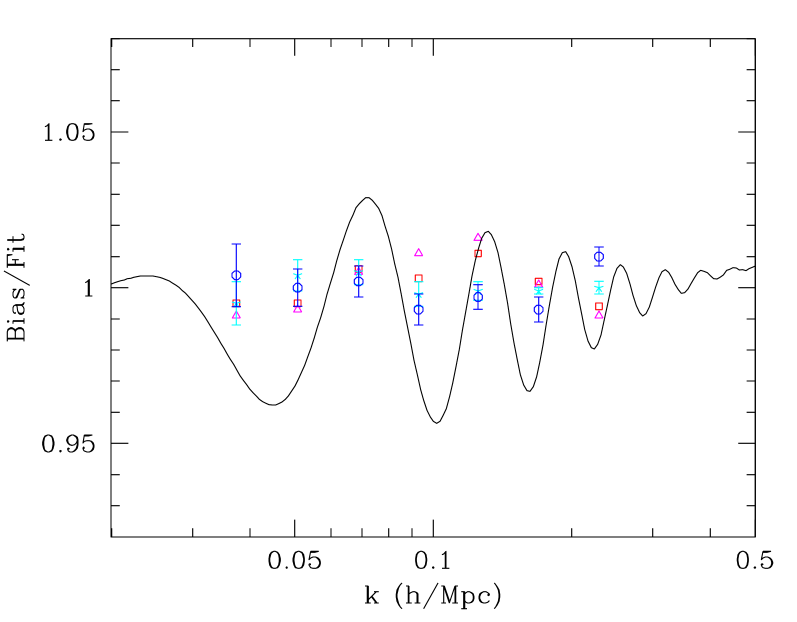
Now we turn to the halo and galaxy catalogues, first in real space. Fig. 8 shows the scale-dependent bias of halos more massive than $M_{\rm min}$ at $z=1$. Here bias is defined as

$$\Delta^{2}_{\rm halo}(k)=b^{2}(k)\Delta^{2}_{\rm dm}(k)$$ (5)

where $\Delta^{2}_{\rm dm}$ is the non-linear dark matter spectrum – the bias thus contains a mix of non-linear and galaxy formation physics. Since the features we are looking for are small, we fit a linear trend (in $\ln k$) to each set of points over the range $k=0.03-0.3\,h{\rm Mpc}^{-1}$ and plot the ratio of the bias to the fit in the lower panel of Fig. 8. What we would like to see is the points being essentially unity.

For the most numerous halos a jackknife estimate suggests that the error bars are smaller than 3% on scales $k>0.03\,h{\rm Mpc}^{-1}$, though the errors are correlated. One must be careful of jackknife estimates on scales approaching the box size, but nonetheless this implies that any structure is smaller than the signal near $k\simeq 0.07\,h{\rm Mpc}^{-1}$ (but may influence the peak positions at the accuracy with which they need to be determined to constrain dark energy). Unfortunately the errors increase as we go to the rarer halos, and for $M_{\rm min}=10^{13.5}\,h^{-1}M_{\odot}$ the errors are 2-7% over the range $k=0.03-0.3\,h{\rm Mpc}^{-1}$. For this reason we switch to the lower resolution runs for the halos with $M_{\rm min}\geq 10^{13}\,h^{-1}M_{\odot}$ and use the dispersion between simulations to estimate the errors.

Figure 9: The galaxy bias, divided by a best fit line, in the interval $0.03<k<0.3\,h{\rm Mpc}^{-1}$, compared to the oscillation signal. The fit is linear in $\ln(k)$ and weights each point equally. Models with $\bar{n}=10^{-3}\,h^{3}{\rm Mpc}^{-3}$ are shown with $\log_{10}M_{1}=13.0$ (circles), $13.5$ (stars), $14.0$ (triangles) and $14.5$ (squares). Two realizations for each of the last 3 models are plotted. For the model with $\log_{10}M_{1}=13$ we use the average of models from the 9 lower resolution runs, plotting the error in the mean rather than multiple realizations.

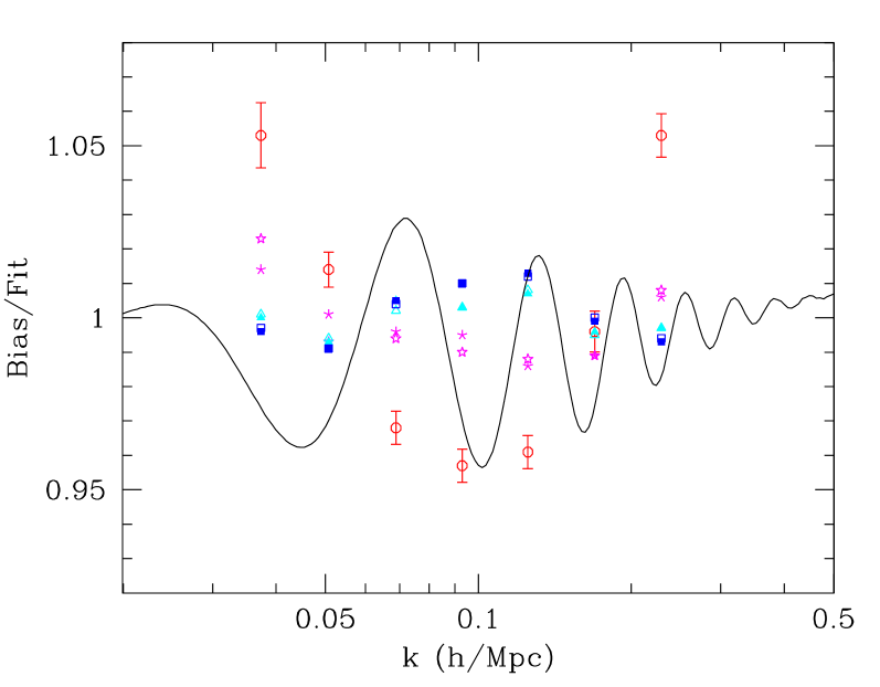
We see in Fig. 8 some curvature remaining after the linear trend is removed. The size of the curvature is small, and could be simply noise from the finite number of modes simulated. It is also possible that this reflects a modulation in the bias of rare halos (which in the peaks formalism PeaksBias depends strongly on the linear mass variance) when compared to the underlying non-linear power of the dark matter. In either case the modulation appears to be smooth, and of lower amplitude than the baryon signal.

Next we show results for some of our galaxy catalogues, with $\bar{n}=10^{-3}\,h^{3}\,{\rm Mpc}^{-3}$. The trend-removed bias is shown in Fig. 9. At the level required for baryon oscillations the bias is clearly not constant, exhibiting curvature once the best-fit line is removed. A comparison of catalogues produced with different random number seeds gives some sense of the error, but only enters in the positions of the satellite galaxies. A jackknife estimate of the errors suggests they are less than 2% in the range $k=0.03-0.3\,h{\rm Mpc}^{-1}$ for all of the models, again with the usual caveat about jackknife errors. For the models with the largest $M_{\rm min}$, which show the biggest curvature, we can use the 9 lower resolution runs to estimate the significance of the curvature. The agreement is fairly good between the average of the 9 low resolution runs and our fiducial model, with the former showing an error around 1% over the $k$-range shown.

Figure 10: The real (open) and redshift (filled) space, halo power spectrum at $z=1$, divided by the featureless linear theory prediction of Ref. EisHu and a constant bias. We show results for the halos most likely to host LRGs, $M_{\rm min}=10^{13}$ (triangles) and $10^{13.5}\,h^{-1}M_{\odot}$ (circles), and for our HOD with $M_{1}=10^{13}\,h^{-1}M_{\odot}$ (squares). The points have been slightly offset (horizontally) for clarity. The stars are the non-linear mass power spectrum from Fig. 6. The solid line is again the linear theory prediction from numerical integration of the coupled Einstein, Boltzmann and fluid equations.

Now we shift to redshift space. The low-$k$ redshift space enhancements for our galaxy and halo catalogues are (fractionally) smaller than for the matter, due to the positive bias of the tracers Kaiser . The models with a satellite galaxy component show a suppression at high-$k$ that begins slightly before that in the matter while the centers of halos show much less suppression, with the real and redshift space power comparable at high-$k$. The latter is due to our assumption that the central halo velocity is the center of mass velocity of the halo. This suppresses the virial motions for these points, and it is the virial motion which leads to the depletion of small-scale power. The actual velocity of central galaxies in halos can be determined observationally from their power spectrum, and is likely to be higher than our center of mass model assumes. Since the power suppression is relatively smooth our approximation will not alter our basic conclusions.

In principle there is more information in the redshift space power spectrum than shown in Fig. 7 because it is no longer isotropic. We shall not investigate this degree of freedom in this paper. Though in principle the information is included in the simulations, our computational volume is too small to allow multiple sub-divisions of the sample while maintaining reasonable significance. For the angle-averaged power spectrum it is clear that on the scales relevant to the oscillations redshift space distortions are a very slowly varying function for $z\geq 1$.

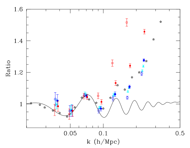
Fig. 10 shows a slightly different view of these results. Here we show the redshift space, galaxy power spectrum at $z=1$ divided by the featureless linear theory prediction of Ref. EisHu and a constant bias fit to the points $0.03\leq k\leq 0.1\,h\,{\rm Mpc}^{-1}$. Superposed is the linear theory prediction from numerical integration of the coupled Einstein, Boltzmann and fluid equations Boltz ; SSWZ . The degree to which these differ shows the level of correction that needs to be applied.

From these studies it appears that a cubic fit (in $\ln k$) to the bias is sufficient to remove the scale dependence of the bias to the percent level in the range $k=0.03-0.3\,h{\rm Mpc}^{-1}$. This deviation is approximately the same size as the error in our calculation. To quantify this better would require more or larger simulations.

5 Conclusions

The coupling of baryons and photons by Thomson scattering in the early universe leads to a rich structure in the power spectra of the CMB photons and the matter. The study of the former has revolutionized cosmology and allowed precise measurement of a host of important cosmological parameters. The study of the latter is still in its infancy, but holds the potential to constrain the nature of the dark energy believed to be causing the accelerated expansion of the universe.

Key to the baryon oscillation program is the ability to compare future observations to theoretical computations of the features in the matter power spectrum. Such calculations are under exquisite control in linear theory SSWZ and the next stage is to explore the effects of non-linear evolution, galaxy biasing and redshift space distortions. Non-linear evolution can be straightforwardly modeled with the current generation of N-body simulations, so the main difficulty lies in understanding or parameterizing galaxy formation.

There have been tremendous advances in our ability to model and understand the relation between galaxies and halos in the last few years. The earlier generation of biasing models MeiWhiPea were highly simplistic, and today we can do significantly better using halo based schemes Halo . Indeed results based on sophisticated modeling of galaxies within halos Millenium or in the limit where the halos are the tracers Ang have already been published. Modeling along similar lines to that done here has recently been reported in Ref. SeoEis05 . Where this is overlap our results are in good agreement.

In this paper we explored a number of phenomenological models for populating halos in PM simulations with galaxies. While unlikely to be correct in any detail these schemes serve to delineate the range of behaviors we might expect in the real universe. We find that non-linearity, galaxy bias and redshift space distortions all introduce important modifications to the basic picture. Both the galaxy bias and the (isotropic) redshift space distortions lead to relatively smooth modulations in power on the scales of interest to baryon oscillations, at least to the level of accuracy we are able to achieve here. The halo and galaxy power spectra exhibit low order structure beyond the acoustic oscillations over the range of scales of relevance. Fitting a cubic polynomial to the ratio of galaxy to dark matter power reduces any remaining structure in the range $0.03\leq k\leq 0.3\,h\,{\rm Mpc}^{-1}$ below the 2% level, comparable to the uncertainty in our calculations. For future, ambitious, surveys even this level of uncertainty may represent a significant piece of the error budget on dark energy properties. Redshift space distortions remain to be explored in more detail. The relative velocity of central galaxies and halos affects the redshift space power spectrum of the former on interesting scales, and has not been well modeled here. In addition there is useful information in the angular structure of the redshift space distortions which we do not have the statistics to explore carefully. We hope to return to some of these issues in a future publication.

Future large redshift surveys offer the opportunity to measure a characteristic scale in the universe: the sound horizon at the time of photon-baryon decoupling. This standard ruler, which we can calibrate from observations of the CMB, may allow us to tightly constrain the evolution of the scale factor and determine the nature of dark energy. To ensure the success of these efforts we need to improve our understanding of the theoretical underpinnings of the method and generate simulated universes which can be used to refine and test our observational strategies.

I would like to thank N. Padmanabhan for conversations and collaboration on marginalizing out “extra physics” in fitting baryon oscillations, S. Habib and K. Heitmann for discussions on initial conditions generation and Chris Blake, Eric Linder and Ryan Scranton for helpful comments on an earlier draft. The simulations were performed on the IBM-SP at NERSC. MJW was supported in part by NASA and the NSF.

References

- (1) D.J. Eisenstein, et al., ApJ, in press.
- (2) P.J.E. Peebles, J.T. Yu, ApJ 162, 815 (1970); A.G. Doroshkevich, Ya.-B. Zel’dovich, R.A. Sunyaev, Soviet Astronomy 22, 523 (1978).
- (3) A. Dekel, ApJ 284, 445 (1984); J.M. Bardeen, J.R. Bond, G. Efstathiou, ApJ 321, 28 (1987); P.J.E. Peebles, ApJ 315, L73 (1987); P.J.E. Peebles, Nature 327, 210 (1987); G.R. Blumenthal, A. Dekel, J.R. Primack, ApJ 326, 539 (1988).
- (4) M. White, D. Scott, ApJ 459, 415 (1995); W. Hu, D. Scott, N. Sugiyama, M. White, Phys. Rev. D52, 5498 (1995); W. Hu, M. White, Phys. Rev. D56, 596 (1997); W. Hu, U. Seljak, M. White, M. Zaldarriaga, Phys. Rev. D57, 3290 (1998);
- (5) U. Seljak, N. Sugiyama, M. White, M. Zaldarriaga, Phys. Rev. D68, 83507 (2003).
- (6) D.J. Eisenstein, W. Hu, J. Silk, A. Szalay, ApJ 494, L1 (1998).
- (7) A. Meiksin, M. White, J.A. Peacock, MNRAS 304, 851 (1999).
- (8) C.L. Bennet, et al., ApJS 148, 1 (2003); G. Hinshaw, et al., ApJS 148, 135 (2003); D.N. Spergel, et al., ApJS 148, 175 (2003).
- (9) A. Cooray, W. Hu, D. Huterer, M. Joffre, ApJ 557, L7 (2001).
- (10) D.J. Eisenstein, in Wide-field multi-object spectroscopy, ASP Conference Series, ed. A. Dey., (2003).
- (11) W. Hu, Z. Haiman, Phys. Rev. D68, 063004 (2003); C. Blake, K. Glazebrook, ApJ 594, 665 (2003); H.-J. Seo, D.J. Eisenstein, ApJ 598, 720 (2003); K. Glazebrook, C. Blake, preprint [astro-ph/0505608].
- (12) M. White, in procedings of the UC Davis meeting on Cosmic Inflation [astro-ph/0305474]
- (13) R. Angulo, et al., preprint [astro-ph/0504456];
- (14) D. Eisenstein, M. White, Phys. Rev. D70, 103523 (2004).
- (15) M. White, MNRAS 321, 1 (2001); U. Seljak, MNRAS 325, 1359 (2001).
- (16) R.J. Scherrer, D.H. Weinberg, ApJ 504, 607 (1998).
- (17) U. Seljak, MNRAS 318, 203 (2000); J.A. Peacock, R.E. Smith, MNRAS 318, 1144 (2000); A. Cooray, R. Sheth, Phys Rep 372, 1 (2002).
- (18) N. Padmanabhan, private communication.
- (19) H.-J. Seo, D.J. Eisenstein, to appear in ApJ [astro-ph/0507338]
- (20) M. Davis, G. Efstathiou, C.S. Frenk, S.D.M. White, ApJ 292, 371 (1985).
- (21) A.E. Evrard, et al., ApJ 573, 7 (2002).
- (22) V. Springel, et al., Nature 435, 629 (2005).
- (23) R. Scoccimarro, R.K. Sheth, MNRAS 329, 629 (2002).
- (24) M. White, ApJS 143, 241 (2002).
- (25) R.K. Sheth, G. Tormen, MNRAS 349, 1464 (2004).
- (26) A.V. Kravtsov, et al., ApJ 609, 35 (2004).
- (27) H.-J. Seo, D.J. Eisenstein, ApJ 598, 720 (2003);
- (28) I. Zehavi, et al., ApJ 621, 22 (2005).
- (29) N. Kaiser, MNRAS 219, 785 (1986).
- (30) J.S. Bullock, R.H. Wechsler, R.S. Somerville, MNRAS 329, 246 (2002).
- (31) D.J. Eisenstein, W. Hu, ApJ 511, 5 (1999).
- (32) N. Kaiser, MNRAS 227, 1 (1987).
- (33) R. Scoccimarro, Phys. Rev. D70, 083007 (2004).
- (34) A. Cooray, MNRAS 348, 250 (2004).
- (35) A. Meiksin, M. White, MNRAS 308, 1179 (1999).
- (36) A. Cooray, W. Hu, ApJ 554, 56 (2001).
- (37) G. Efstathiou, et al., MNRAS 235, 715 (1988); S. Cole, N. Kaiser, MNRAS 237, 1127 (1989); H.J. Mo, S.D.M. White, MNRAS 282, 347 (1996).