WINGS: a WIde-field Nearby Galaxy-cluster Survey. I:
Optical imaging

This is the first paper of a series that will present data and scientific results from the WINGS project, a wide-field, multiwavelength imaging and spectroscopic survey of galaxies in 77 nearby clusters. The sample was extracted from the ROSAT catalogs of X-Ray emitting clusters, with constraints on the redshift ($0.04<z<0.07$) and distance from the galactic plane (${|}b{|}\geq$20 deg).

The global goal of the WINGS project is the systematic study of the local cosmic variance of the cluster population and of the properties of cluster galaxies as a function of cluster properties and local environment. This data collection will allow the definition of a local, ’zero-point’ reference against which to gauge the cosmic evolution when compared to more distant clusters.

The core of the project consists of wide-field optical imaging of the selected clusters in the $B$ and $V$ bands. We have also completed a multi-fiber, medium-resolution spectroscopic survey for 51 of the clusters in the master sample. The imaging and spectroscopy data were collected using, respectively, the WFC@INT and WYFFOS@WHT in the northern hemisphere, and the WFI@MPG and 2dF@AAT in the southern hemisphere. In addition, a NIR ($J$,$K$) survey of $\sim$ 50 clusters and an $H_{\alpha}+U$ survey of some 10 clusters are presently ongoing with the WFCAM@UKIRT and WFC@INT, respectively, while a very-wide-field optical survey has also been programmed with OmegaCam@VST.

In this paper we briefly outline the global objectives and the main characteristics of the WINGS project. Moreover, the observing strategy and the data reduction of the optical imaging survey (WINGS-OPT) are presented. We have achieved a photometric accuracy of $\sim$0.025 mag, reaching completeness to V$\sim$23.5. Field size and resolution (FWHM) span the absolute intervals (1.6-2.7) Mpc and (0.7-1.7) kpc, respectively, depending on the redshift and on the seeing. This allows the planned studies to obtain a valuable description of the local properties of clusters and galaxies in clusters.

1 Introduction

Galaxies of different morphology are not evenly distributed. It is now more than 70 years since Hubble & Humason (1931) first noticed that (in the local universe) spiral galaxies are abundant in the field while S0 and elliptical galaxies dominate in denser regions. Gravitational interaction apparently affects the global properties of the galaxies even in low density environments, and even such field galaxies show significant differences with respect to truly isolated systems that have been free of interaction for a long period of time (Varela et al. 2004).

Clusters of galaxies are dense peaks in the galaxy distribution and therefore appropriate sites to look for changes in the properties of the galaxies. They can be therefore used to trace the evolution of the systems themselves as well as that of the galaxies in them. Such a systematic analysis certainly needs a fair knowledge of the properties of local clusters of galaxies and their content (the end point of the evolution), extensive enough to cope not only with the average properties but also with their physical variance. This is unfortunately still lacking. As a matter of fact, while a large amount of high quality data for distant clusters is continuously being gathered from both HST observations and large ground-based telescopes, our present knowledge of the systematic properties of galaxies in nearby clusters, remains surprisingly limited, with Virgo, Coma and Fornax as the main references.

In the range 0.4$\leq z\leq$0.5, exploiting the high spatial resolution achieved with the Hubble Space Telescope (HST), Dressler et al. (1997) and Smail et al. (1997) found that spirals are a factor of 2-3 more abundant and S0 galaxies are proportionally less abundant than in nearby clusters, while the fraction of ellipticals is already as large or larger. This implies significant morphological transformations occurring rather recently. Similarly, using excellent-seeing, ground based imaging with the NOT telescope (La Palma), Fasano et al. (2000) completed the picture in the range 0.1 $\leq z\leq$ 0.25, showing that the S0 population smoothly grows from $z\sim 0.5$ to $z\sim 0$, at the expense of the population of spiral galaxies. They also highlighted the role that the cluster type plays in determining the relative occurrence of S0 and elliptical galaxies at a given redshift: clusters at $z\sim 0.1-0.2$ have a low (high) S0/E ratio if they display (lack) a strong concentration of elliptical galaxies towards the cluster centre. This dichotomy seems to support Oemler’s (1974) suggestion that elliptical-rich and S0-rich clusters are not two evolutionary stages in cluster evolution, but intrinsically different types of clusters in which the abundance of ellipticals was established at redshifts much greater than $0.5$.

That trend is supported by the morphological studies at $z>0.5$, that find an even lower fraction of early-type galaxies (Es+S0s), thus indicating that this fraction keeps decreasing up to $z\sim 1$ (van Dokkum et al. 2000; Lubin et al. 2002, Simard et al.  private communication). The most recent works, based on the Advanced Camera for Surveys, demonstrate that it is the decreasing proportion of S0 galaxies that drives this decline also at $z\sim 0.8-1$ (Postman et al. 2005, Desai et al.  in preparation). This change of the morphological mix in clusters is expressed in the evolution of the morphology-density relation with $z$ (Dressler et al. 1997; Postman et al. 2005).

The work on intermediate-redshift clusters observed by HST has been complemented with ground-based spectroscopic surveys that have led to a detailed comparison of the spectral and morphological properties (Dressler et al. 1999; Poggianti et al. 1999; Couch et al. 1994, 1998, 2001; Fisher et al. 1998; Lubin et al. 1998; Balogh et al. 1997, 2000). These studies have shown that the spiral population includes most of the star-forming galaxies, a large number of post-starburst galaxies and a sizeable fraction of the red, passive galaxies; in contrast, the stellar populations of (the few) S0 galaxies appear to be as old and passively evolving as those in the ellipticals. These observations are consistent with the post-starburst and star-forming galaxies being recently infallen field spirals whose star formation is truncated upon entering the cluster and that will evolve into S0’s at a later time.

At variance with intermediate redshift clusters, for which recent, high-quality photometric data are available, the morphological reference for local clusters is still the historical database of Dressler (1980), based on photographic plates, giving the positions, the estimated magnitudes (down to $V\sim 16$) and the visual morphological classification for galaxies in 55 clusters in the range 0.011 $\leq z\leq$ 0.066. This awkward situation can be easily understood since only with the new large format (wide-field) CCD mosaic cameras a significant number of low redshift clusters could be reasonably well mapped.

Our goal has been to help fill this information gap. Accordingly, we began in 1999 a program to secure a large database for a local sample of clusters, to study the cosmic variance of the cluster properties and their populations in a systematic way. The result would be a reference ’zero-point’ for comparison with studies at higher $z$ and for evolutionary studies. To that end we have collected wide-field photometric and spectroscopic data for an X-ray selected sample of 77 clusters at low redshift, spanning a wide range in X-ray and optical properties. The observational requirements have been set to ensure an adequate data quality, both for imaging and spectroscopy, in order to obtain detailed and reliable morphological classifications and estimates of stellar population ages, metallicities and star formation histories.

Similar projects were, in the meantime, also begun, either for smaller samples (Pimbblet et al. 2001; Christlein & Zabludoff 2003), or with more limited goals (Smith et al. 2004; Nelan et al. 2005). On the spectroscopic side, the ESO Nearby Abell Cluster Survey (Katgert et al. 1996; Biviano et al. 1997, ENACS) collected redshifts for galaxies in 107 clusters, of which 67 with at least 20 spectroscopic members. This dataset yielded information on cluster velocity dispersions, kinematics and spatial distributions of different types of galaxies, that motivated detailed analysis of cluster properties (Katgert et al. 2004; Biviano et al. 1997, 1999; Mazure et al. 1996). Samples of low-redshift clusters have been also identified based on the redshifts obtained by two recent large spectroscopic surveys, 2dF and Sloan (De Propris et al. 2003; Nichol 2004; Vogeley et al. 2004), the former having no corresponding CCD imaging database. Results based on these surveys have highlighted the strong correlation between star formation properties in galaxies and local galaxy density, and that such a correlation exists both inside and outside of clusters (Lewis et al. 2002; Gómez et al. 2003; Kauffmann et al. 2004; Balogh et al. 2004). Unfortunately, given the typical spatial resolution of the imaging data and the magnitude limit of the SDSS, it is not immediately possible to make a detailed comparison with the existing high redshift morphological and spectroscopic studies.

This paper is the first of a series presenting the results of this project, that we have called WINGS for WIde-field Nearby Galaxy-cluster Survey. The goal of the present paper is to outline the objectives and the main characteristics of the WINGS program (Section 2) and to describe in detail the optical imaging observations. The selection of the cluster sample is presented in Section 3, while Section 4 is devoted to the description of the observations and the procedures for the reduction of the optical wide-field survey (WINGS-OPT). The data quality of optical imaging is analysed in Section 5. Finally, a brief summary of the future plans concerning the whole WINGS project is given in Section 6.

In this and in the following papers of the series we assume the now standard metric with $H_{0}$=70, $\Omega_{m}$=0.3 and $\Omega_{\Lambda}$=0.7.

2 The WINGS project

Figure 1: All-Sky Aitoff map of the cluster sample (equatorial coordinates). Lines delimiting the region $|b|\leq$20 are drawn.

The principal goal of the WINGS project is to elaborate a statistically meaningful, high quality database of the properties of nearby clusters of galaxies and of the galaxies that populate them. Hopefully, this will serve to improve our knowledge of clusters and cluster galaxies in the local universe and will provide the reference to gauge the changes with redshift over their physical variance at a given $z$.

In broad terms, the goals of the project are to characterize the global properties of clusters taken as systems, and those of their member galaxies. Among the former, besides the already existing data on the X-ray luminosity, we include their total luminosity and size, the velocity dispersion, the presence of substructures and the cluster scaling relations (Marmo et al. 2004). This will allow us to explore the existence of well defined relations among structural parameters and characterize the actual range of those properties.

Regarding the member galaxies, our primary goals are to analyze the variance of the morphological fractions (E/S0/S/Irr), their distribution in the clusters and the morphology-density relation. The analysis of the colors and the spectral information will provide the data necessary to retrace the star formation history of galaxies in nearby clusters.

The WINGS project was designed to cover all these topics. Originally it was planned as a wide-field optical ($B$,$V$) imaging survey. This is the core of the project, hereafter called WINGS-OPT. The strategy for imaging and for the resulting data reduction are the main subject of the present article.

In addition, other surveys were designed and carried out to complement the characterization of the cluster galaxies. The already completed WINGS-SPE survey consists of multi-fiber spectroscopy of galaxies in 51 clusters from the master WINGS sample, obtained with the WYFFOS@WHT and the 2dF@AAT spectrographs over the same area covered by the optical imaging ($34^{\prime}\times 34^{\prime}$). The spectra cover the range 3800-7000 Å  (WYFFOS) and 3600-8000 Å  (2dF), with dispersions of 3Å and 9Å, respectively, for the galaxies with $V<20$ (between 100 and 300 per cluster). This limit is 1.5 and 2.0 mag deeper than the 2dF and Sloan surveys, respectively.

Three more follow-up surveys of clusters in the WINGS sample are presently ongoing. The first one is a NIR (WINGS-NIR: $J$ and $K$-bands) imaging survey, with the new Wide-Field Camera at the 3.8 m UKIRT telescope. This will obtain data for $\sim 50$ clusters, useful at providing an estimate of the stellar mass of galaxies, as well as constraining the spectral energy distribution of galaxies in these fields. The other ones are $H_{\alpha}$ and U-broad-band surveys (WINGS-HAL and WINGS-UV, respectively), with the WFC@INT camera and purpose-defined narrow-band filters (for the WINGS-HAL survey), to image $\sim$1 square degree of 10 WINGS clusters. Finally, a very-wide-field ($\sim$1 square degree) optical survey (WINGS-VWF), with the ESO-VST telescope, equipped with OmegaCam, has been programmed for the near future.

In combination, these data will constitute a multiwavelength photometric and spectroscopic dataset which will allow detailed studies of the properties of nearby Clusters of Galaxies, and cope with their variance, necessary to identify the cosmic evolution when compared with those of higher redshift systems.

We present here the observations, data reduction and analysis of data quality from WINGS-OPT. For all galaxies down to the limit of detectability we have extracted the position, size, concentration, average flattening and orientation, as well as the integrated and aperture photometry in the two observed bands, $B$, $V$. For a subsample of large galaxies we have also obtained detailed surface photometry (luminosity and geometrical profiles) and global structural parameters (total magnitudes, effective radii, ellipticity and Sérsic index) using our automatic surface photometry tool GASPHOT (Pignatelli et al. 2005). Finally, morphological type estimates of the same subsample of large galaxies, compared and calibrated with visual classifications, were automatically obtained with the purpose-written tool MORPHOT (Fasano et al. 2005).

The catalogues and the statistical analyses of galaxies and cluster properties will be presented in subsequent papers of this series. To maximize the scientific outcome of the data, the whole WINGS dataset and products, including photometry, surface photometry, morphological and spectroscopic catalogs, will become publicy available as the corresponding papers of this series are published.

3 The cluster sample

Figure 2: Distribution of some cluster properties in the WINGS sample

To investigate in a systematic way the correlations between cluster properties and cluster galaxy populations, a well-defined, large cluster sample is required, with available X-ray data and covering a wide range in optical and X-ray properties.

WINGS clusters have been selected from three X-ray flux limited samples compiled from ROSAT All-Sky Survey data: the ROSAT Brightest Cluster Sample (Ebeling et al. 1998, BCS), and its extension (Ebeling et al. 2000, eBCS) in the Northern hemisphere and the X-Ray-Brightest Abell-type Cluster sample (Ebeling et al. 1996, XBACs) in the Southern hemisphere. These catalogs are uncontaminated by non-cluster X-ray sources (AGNs or foreground stars). The BCS is 90% complete for fluxes higher than $4.4\times 10^{-12}\,\rm erg\,cm^{-2}\,s^{-1}$ in the 0.1-2.4 keV band. The eBCS extends the BCS down to $2.8\times 10^{-12}\,\rm erg\,cm^{-2}\,s^{-1}$ with 75% completeness. Finally, the XBACs is an essentially complete sample of Abell clusters with fluxes above $5.0\times 10^{-12}\,\rm erg\,cm^{-2}\,s^{-1}$.

The original WINGS sample comprises all clusters from BCS, eBCS and XBACs with a high Galactic latitude ($|b|\geq 20$ deg) in the redshift range $0.04<z<0.07$. The redshift cut and the Galactic latitude are thus the only selection criteria applied to the X-ray samples. The redshift range has been chosen to guarantee both a large area coverage (the side of our field is $34^{\prime}\geq 1.6\,\rm Mpc$) and sufficient spatial resolution ($1^{\prime\prime}\leq 1.3\,\rm kpc$) for all clusters.

After having removed the cluster A3391, because of the presence of strong non-uniform illumination in the CCD frames, the final WINGS sample includes 77 clusters (41 in the Southern Hemisphere and 36 in the Northern Hemisphere, see Figure 1), of which 18 are in common with Dressler’s (1980) sample. This partial overlap is useful for comparing the two datasets and the morphological classifications. Table WINGS: a WIde-field Nearby Galaxy-cluster Survey. I: Optical imaging (Online Material) lists the cluster name, coordinates of the adopted center, redshift, Abell richness, Bautz-Morgan type, X-Ray luminosity from Ebeling et al. (1996,1998,2000; converted to our cosmology) in units of $10^{44}$ erg $s^{-1}$ and color excess E(B-V).

The WINGS clusters span a wide range in X-ray luminosities ($\rm log\,L_{X}[0.1-2.4\,keV]=43.2-44.7$), corresponding to $\sim 5\times 10^{14}\rm\,to\,>10^{15}$ gravitational solar masses (Reiprich & Bohringer 2002), as well as in optical properties such as Abell richness and Bautz-Morgan type (see Figure 2).

Table 1: The WINGS-OPT observing runs

WFC INT-2.5m (North)
Run number	PATT/CAT REF.	Starting Date	Alloc.Time	$B$ Filt.ID	$V$ Filt.ID
1	C3	Aug. 28, 2000	1 night	Harris (191)	Harris (192)
2	ITP3	Apr. 25, 2001	5 nights	Kitt Peak (210)	Harris (192)
4	ITP3	Sep. 15, 2001	3 nights	Harris (191)	Harris (192)
WFI MPG/ESO-2.2m (South)
Run number	Proposal ID	Starting Date	Alloc.Time	$B$ Filt.ID	$V$ Filt.ID
3	67.A-0030	Aug. 15, 2001	2 nights	ESO99 (842)	ESO89 (843)
5	68.A-0139	Feb. 14, 2002	30 hrs	ESO99 (842)	ESO89 (843)
6	69.A-0119	Apr. 01, 2002	18 hrs	ESOnewB (878)	ESO89 (843)

4 WINGS-OPT survey

4.1 Survey requirements

Figure 3: Distribution of effective diameters (in kpc) for early-type galaxies in the nearby clusters studied by Fasano et al. (2002). The dotted line corresponds to 1.5 kpc in our cosmological framework.

Among the attributes of any photometric galaxy survey, the most important ones concern the spatial resolution and the photometric depth. Concerning the former, Figure 3 shows the distribution of effective diameters (in kpc) for early-type galaxies in the nearby clusters studied by Fasano et al. (2002). Since a good galaxy profile restoration is usually possible down to effective diameters of the order of the Full Width Half Maximum (FWHM) of the point spread function (see Figure 4 in Fasano et al. 2002), we chose as the WINGS-OPT imaging requirement that the FWHM not exceed $\sim$1.5 kpc in our cosmological framework (the dotted line in Figure 3).

Concerning the photometric depth, our interest is twofold: First, we want the WINGS-OPT survey to be able to sample the luminosity function of clusters down to the dwarf galaxies ($M_{V}\sim$ -14). Second, we require that the depth is sufficient to allow a reliable surface photometry (S/N ratio $\approx$4.5 per square arcseconds) down to a surface brightness of $\mu_{V}\sim$25 mag arcsec^-2. Section 5 illustrates to what extent the above mentioned requisites have been fulfilled by the WINGS-OPT observations.

4.2 Observations

The observations of the WINGS-OPT survey have been taken in dark time with the Wide Field Camera (WFC) mounted at the corrected f/3.29 prime focus of the INT-2.5m telescope in La Palma (Canary Islands, Spain) and with the Wide Field Imager (WFI) mounted at the f/8 Cassegrain focus of the MPG/ESO-2.2m telescope in La Silla (Chile) for the northern and southern clusters, respectively. The northern campaign consisted of three runs, totalling 9 nights, during which 46 clusters were observed. The southern campaign has produced data for 35 clusters during three observing runs (the last two in service mode), for a total of 2 nights in observer mode, plus about 48 hours of science exposures in service mode. Tables 1 and  2 list the observing runs of the WINGS-OPT survey and the main instrumental characteristics of the wide-field cameras, respectively.

Table 2: Technical features of the wide-field cameras used by the WINGS-OPT survey

Feature	WFC@INT	WFI@MPG
Field of view	$34^{\prime}\times 34^{\prime}$	$34^{\prime}\times 33^{\prime}$
Pixel scale	0.33′′/pixel	0.238′′/pixel
Detector	$4\times 2k\times 4k$	$8\times 2k\times 4k$
Filling factor	$93.6\%$	$95.9\%$
Read-out noise	$6.2\leavevmode\nobreak\ e^{-}$/pix	$4.5\leavevmode\nobreak\ e^{-}$/pix
(Inverse) gain	$2.8\leavevmode\nobreak\ e^{-}/ADU$	$2.0\leavevmode\nobreak\ e^{-}/ADU$
Full-well capacity	$\sim 180,000\leavevmode\nobreak\ e^{-}$	$>200,000\leavevmode\nobreak\ e^{-}$
Telescope aperture	$2.54\leavevmode\nobreak\ m$	$2.20\leavevmode\nobreak\ m$
Telescope focus	Prime focus	Cassegrain

Figure 4: Transmission curves of the filters used in the WINGS-OPT survey

We decided to take images in the $V$ and $B$ bands. The V filter allows us to compare our results with previous studies of nearby clusters, as well as with WFPC2/ACS@HST ($F814W$) studies of clusters at $z\sim$0.5. The B filter is needed in order to get colors of galaxies and especially useful because it is the rest-frame equivalent to the imaging of clusters at $z\geq$0.5 done using HST + ACS. Table 1 reports the identifications of the broad band $B$ and $V$ filters used in the different WINGS-OPT observing runs, while in Figure 4 the transmission curves of the different filters are shown.

With the average (dark time) observing conditions at both WFC@INT and WFI@MPG, it turns out that the photometric depth we require for the survey (see Section 4.1) can be fulfilled with exposure times of the order of 20-25 minutes, depending on the photometric band.

In order to avoid saturation of the brightest objects, usually three exposures per filter have been obtained, also allowing us to easily remove cosmic rays. For A3528b (run #5) we have just one exposure per filter (3m and 8m in the $B$ and $V$ band, respectively).

We aimed for similar FWHM for each of the summed exposures. Thus, whenever possible we tried to take these exposures with a short interval between them. Obviously, this was not always the case for clusters observed in service mode (runs #5 and #6 with WFI@MPG). In particular, for nine clusters observed during the run #6 (A2382, A2399, A2717, A2734, A3667, A3716, A3809, A3880 and A4059), we got from ESO two medium seeing, long exposures and a good seeing, short exposure per filter. In a forthcoming paper of the series we will exploit this occurrence to check the dependence of the surface photometry on the seeing.

During the first observing run we explored with a single cluster (A2107) the possibility of taking three shifted exposures per filter in order to fully sample the gaps between CCDs. After mosaicing, however, we verified that, due to the worsening of the S/N ratio within the underexposed regions, this procedure resulted in a net loss of the area usable to perform deep surface photometry. Thus, we decided to abandon this technique. Instead, for the whole of run #4, and for many clusters observed in service mode during runs #5 and #6, a small shift in right ascension ($\sim$25pix.) was applied, allowing us to remove bad pixels and columns.

In order to provide the WINGS-OPT survey with accurate astrometric solutions and background galaxy counts estimation for both WFC@INT and WFI@MPG cameras, we have also imaged the astrometric regions ACR-D/E/M/N from Stone et al. (1999) and a blank field in each hemisphere.

Finally, some dark and dome-flat exposures and several bias frames, twilight sky-flats and photometric standard fields have been obtained for each observing night.

Table WINGS: a WIde-field Nearby Galaxy-cluster Survey. I: Optical imaging (Online Material) reports the observing log of the WINGS-OPT survey.

4.3 Basic Reduction

Most of the steps required to reduce the data coming from mosaic wide-field cameras are similar to those usually performed on traditional CCD frames. However, the use of such a wide area mosaic raises a number of new technical issues, mainly related to the presence of geometric distortions and photometric differences between the different CCDs. In addition, handling the huge number of pixels from these kind of cameras requires that even the standard reduction procedures must be revised, to make them more efficient. In Appendix A (see Online Material) the details of the basic reduction procedures are given. Here we just mention that the photometric uncertainties due to the flat fielding are expected to be less than 1% (0.01 mag, see Section A.3), while those arising from bias removal and linearity correction are likely to be negligible. In Appendix A we also show that, as far as the astrometry is concerned, the accuracy of the WINGS-OPT survey is of the order of 0.2 arcseconds, in the worst centering situation (big galaxies; see Section A.4 and Figure 14).

4.4 Photometric Calibration

Since the CCDs of any mosaic camera have usually different zero points and color responses, the optimal standard fields for WF imaging should map each CCD with a sufficient number of stars covering wide ranges of both magnitude and color. For this reason, the problem of photometric calibration in wide-field CCD mosaic cameras is not yet solved satisfactorily. Nowadays there are two main sets of standard fields that, even if they not provide a complete coverage of the CCD mosaic, can be used satisfactorily for wide field photometry, namely the sample of Landolt (1992) and that of Stetson (2000). We preferred to use the Landolt sequences, since Stetson’s standard fields, which go even deeper than the Landolt fields (typically fainter than 14th magnitude, with a larger number of standard stars), normally cover no more than 20 arcmin on a side. Actually, NGC 6633 was the only Stetson standard field we used for our calibration (run #4). We used the same set of Landolt SA fields through both the INT and the MPG observing runs, namely SA 92/95/98/101/104/107/110/113. During each night two or three SA fields were observed at different zenith distances in order to map the atmospheric extinction. However, the long average duration of each cluster pointing made it difficult (often impossible) to observe the same standard field more than twice per night. In addition, the small number of stars usually present in the standard star fields often makes it impossible to photometrically calibrate each CCD in a single calibration frame.

Thus, we have performed the photometric calibration using a self-consistent method, taking advantage of all the standard fields in each observing run. Section B.1 (Online Material) reports both the formalism of this method and the calibration coefficients we obtained. In particular, Figure 15 shows, for each observing run and for all observations of the standard stars, the residuals (given by eq. 4) of our photometric calibration in the two bands as a function of both standard magnitudes and colors. Excluding from the calibration set the saturated and blended stars and using a recursive $k-\sigma$ procedure to remove the outliers, the typical $r.m.s$ of the residuals we achieved with our calibration is of the order of $\sim$0.025 mag (see Tables 3 and  4).

Table 3: Total $r.m.s.$ and sky transparency contribution to the $r.m.s.$ of the residuals of the photometric calibration in the two bands for each observing run of the WINGS-OPT survey.

Run	$\sigma_{\Delta B}$		$\sigma_{\Delta V}$
	Total	Sky Transp.	Total	Sky Transp.
#1	0.020	0.010	0.017	0.007
#2	0.023	0.014	0.018	0.007
#4	0.022	0.009	0.026	0.014
#3	0.034	0.020	0.028	0.016
#5	0.026	0.016	0.023	0.013
#6	0.030	0.022	0.026	0.018

To try and disentangle the different contributions to the total $r.m.s$, we have analysed different nights of the same run. In Table 3, the right column relative to each filter reports the contribution to the scatter arising from sky transparency fluctuations through the run. In particular, the night-, run- and long-term contributions to these fluctuations, estimated normalizing the residuals relative to each individual star to their night-, run- and long-term averaged values, respectively, are found to be roughly equivalent among each other. However, from Table 3 it is clear that the different contributions due to sky transparency variations, altogether, do not represent the dominant share of the scatter in the photometric calibration. This is likely due to systematic effects arising from both possible zero point gradients across the fields and differences among the photometric systems.

Concerning the former effect, in Appendix A (Section A.3) we report on the non-uniform illumination of the imaging taken with WFI@MPG, which can induce systematic magnitude differences up to $\sim$0.1 mag across the field. Even though our chip by chip photometric calibration procedure (see Table 5 in Appendix B) should in principle alleviate this problem, we have directly verified the non-uniformity of our photometric zero points by plotting in Figure 5 (left panels) the residuals of our calibration versus the pixel coordinates for the whole set of standard stars observed with WFI@MPG. Since in both filters a significant dependence on the position is found to persist for the residuals, we have interpolated them through the field using a 2nd-order, 2D polynomial. The right-hand panels of Figure 5 show that the residuals, after correction, no longer depend on the position.

Figure 5: Residuals of our calibration versus the pixel coordinates, for the whole set of standard stars observed with WFI@MPG, before (left panels) and after (right panels) correction

No significant spatial gradients of the residuals of the photometric calibration were found in the case of the WFC@INT camera. Table 4 summarizes the different contributions to the scatter, averaged over the whole data-set of standard stars observations available for each camera.

Table 4: Different contributions to the $r.m.s.$ of the residuals of the photometric calibration in the two bands and for each WF camera

Contribution	WFC@INT		WFI@MPG
	$\sigma_{\Delta B}$	$\sigma_{\Delta V}$	$\sigma_{\Delta B}$	$\sigma_{\Delta V}$
Sky Transp.	0.013	0.011	0.019	0.015
Phot.Syst.	0.018	0.020	0.018	0.016
ZP Gradient	-	-	0.010	0.010
Total	0.022	0.023	0.028	0.024

4.5 Mosaics

After having gone through the usual reduction steps (de-biasing, linearity correction, flat-fielding, astrometry), the multi-extension exposures of each given cluster in each filter have been registered, co-added and mosaiced using the wfpred package (see Appendix A).

Figures 6 and 7 show examples of the mosaic imaging obtained with the WFC@INT and WFI@MPG cameras, respectively. We produced co-added and mosaiced frames even when the different exposures of a given cluster came from different observing nights, with different observing conditions. However, in these cases, the mosaics of just the exposures with comparable conditions were produced. For instance, when two medium seeing, long exposures and a good seeing, short exposure were available in each filter (five clusters observed during run #6; see Section 4), besides the co-added mosaic of the three exposures, we produced that of the two medium seeing exposures and the mosaic of the good seeing exposure. In fact, each one of them could be suitable for a particular task (integrated photometry, surface photometry, morphology).

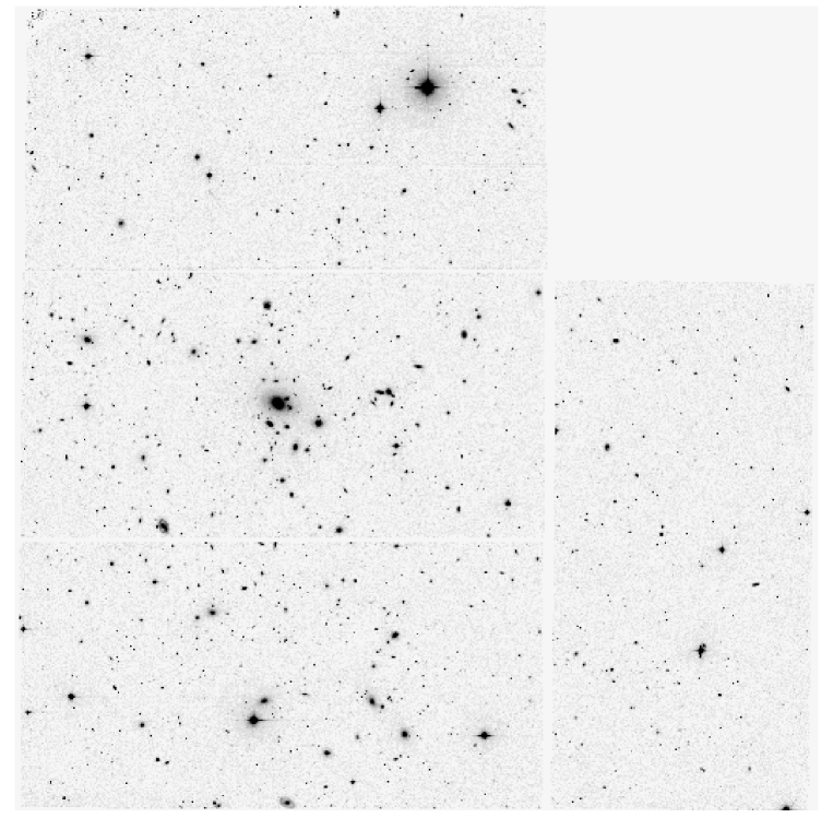
Figure 6: Mosaic of the WFC@INT image of the cluster A151. North is up, East is left. The field of view is $34^{\prime}\times 34^{\prime}$.

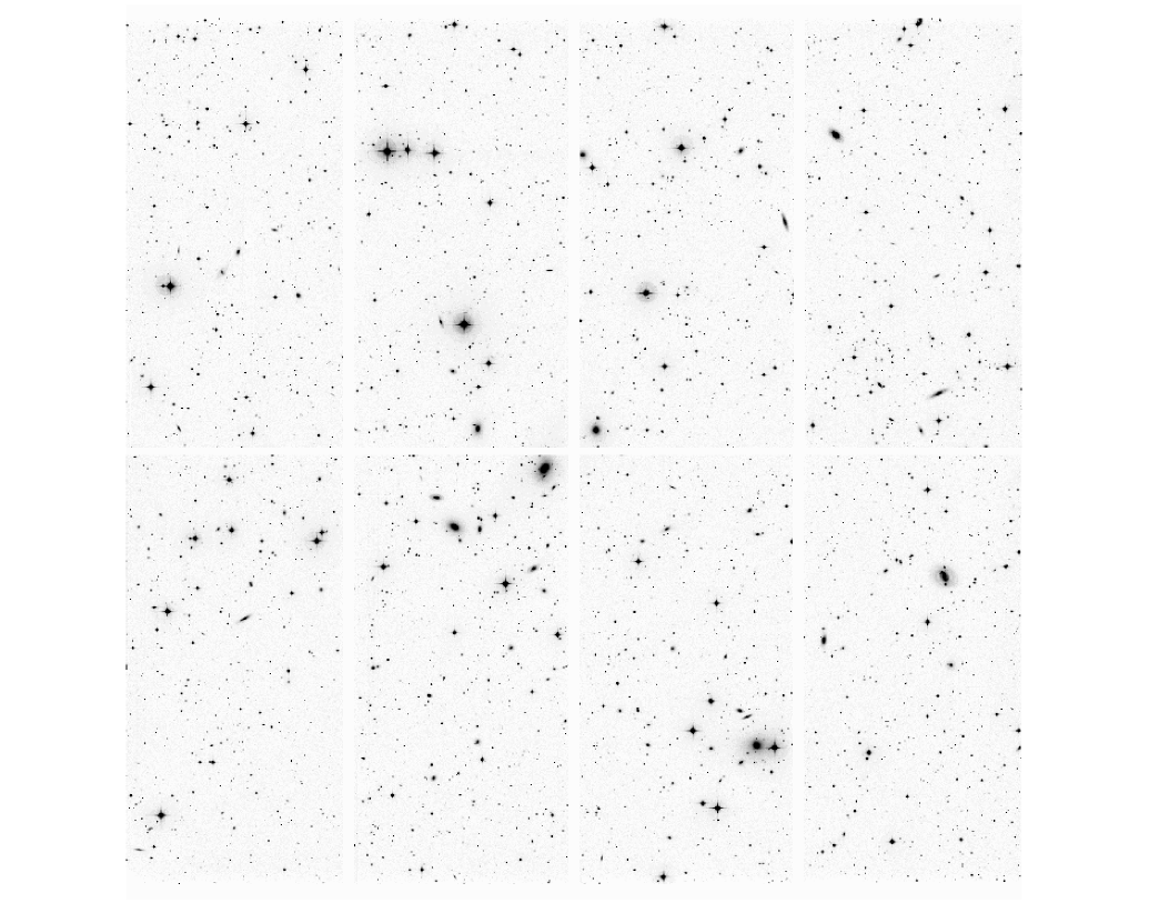
Figure 7: Mosaic of the WFI@MPG image of the cluster A3556. North is up, East is left. The field of view is $34^{\prime}\times 33^{\prime}$.

Before extracting the photometric quantities to be included in our catalogs (Section 4.8), we have put the co-added mosaic frames through a normalization procedure accounting for the different photometric coefficients of the mosaic’s CCDs. This procedure is described in Section B.2 (Online Material).

4.6 Cosmetics

Since for each cluster three exposures, with a short interval between them, were usually obtained for each filter (see Section 4.2), the co-adding procedure was in general sufficient to remove cosmic rays. When less than three close exposures were available, we resorted to the IRAF tool COSMICRAYS to do the job.

For nearly half of the cluster sample (run #4 and part of runs #5 and #6) the three available exposures were dithered by $\sim$25 pixels, allowing us to remove the bad pixels and columns. For the remaining clusters, pixel mask images were automatically produced and used by the IMEDIT-IRAF tool to interpolate the bad regions. We were forced to adopt this technique because of the noticeable worsening of the photometric accuracy we found in the experiments carried out with SExtractor (Bertin & Arnouts 1996) when weight-images are used to account for bad pixels and columns.

4.7 Background removal

Estimating the local background is a crucial step in achieving good quality photometry. In our case, the main problems related to the background removal reside in the presence of objects with extended halos (big early-type galaxies) or wings (very bright stars), as well as in the discontinuity of the background associated with the gaps between different CCDs. Both are likely to produce artificial distortions in the background map, thus systematically biasing the local backgrond estimates.

We exploited the capabilities of SExtractor, as well as the ELLIPSE-IRAF tool to devise a semi-automatic, iterative procedure for optimal sky subtraction over CCD mosaics, even in case of crowded galaxy cluster fieds, possibly including big halo galaxies and/or very bright stars. This procedure generates two images. The first is the original mosaic, after model subtraction of the big halo galaxies and very bright stars. The second image contains only the previously removed big/bright galaxies, where the masked pixels (neighbours or gaps) are replaced by the models. These two images are suitable for SExtractor processing, since each one of them contains homogeneously sized objects, without critical blendings.

4.8 Catalogues

Figure 8: The FWHM in arcseconds versus the physical size this projects to at the cluster redshift, with the marginal distributions for each, for the WINGS-OPT imaging. Filled and open circles indicate that the best FWHM is achieved in the $V$ and $B$ band, respectively.

Figure 9: Apparent versus absolute $V$-band magnitudes at the detection limit, with the marginal distributions for each, for our WINGS-OPT observations. Different observing runs are plotted with different symbols: full and open symbols referring to the WFC@INT and WFI@MPG observations, respectively.

The final photometric catalogs of the WINGS-OPT survey are obtained, for each cluster, by running SExtractor over the two previously described images in both wavebands and by merging the four resulting catalogs into a single master-catalog containing all the sources detected in both filters over the field. The magnitudes in the final catalogs are color corrected following the procedure outlined in Section B.2 (equations 7 and 8).

At this stage, we tried to detect as many sources as possible by adopting very liberal detection parameters within SExtractor. In particular, we used a minimum detection area of 5 pixels and detection thresholds of 1.5 and 1.1 times the $\sigma_{bkg}$ for the WFC@INT and WFI@MPG imaging, respectively, roughly corresponding to S/N$\approx$4.5 per square arcseconds in both cases.

In a forthcoming paper of the WINGS series, we will present the WINGS-OPT catalogs, describing in detail the procedure we used to produce them. Here we just mention that, on the basis of the automatic star/galaxy classifier (S/G) given by SExtractor, the master catalog for each cluster was split into three preliminary catalogs: (i) a galaxy catalog (GCAT, S/G$\leq$0.2); (ii) a star catalog (SCAT, S/G$\geq$0.8); (iii) a catalog of objects with uncertain classification (UCAT, 0.2$<$S/G$<$0.8). Finally, with the use of the multi-aperture photometry plotting tools and our visual inpsections of the final images, the catalogs are carefully cleaned, with spurious detections (residual spikes and bad pixels, border effects, etc..) removed and mis-classified objects moved from one catalog to another (GCAT into SCAT and viceversa).

5 The WINGS-OPT data quality

In Section 4.1 we set the minimal requirements that the WINGS-OPT imaging survey should obey as far as both the spatial resolution (FWHM$\leq$1.5 Kpc) and the limiting absolute magnitude ($M_{V}^{lim}\geq-14$) are concerned. Using the photometric catalogues we have checked to what extent these requirements have been fulfilled by the actual WINGS-OPT data.

5.1 Spatial resolution

In Figure 8 the FWHM in arcseconds is plotted against the actual physical resolution this projected to at the redshift of the cluster (expressed in kpc), for all our WINGS-OPT observations. Apart from a few very bad cases, the bulk of our cluster sample, in both arcseconds and kiloparsecs, is located around FWHM$\sim$1.1 (see histograms in the figure). In spite of the repeated observations taken in different runs, the spatial resolution of two clusters (A1668, A2626) largely exceeds the requirement described in Section 4.1. These clusters will be flagged out in the statistical analyses of surface photometry and morphology results.

5.2 Photometric depth

Figure 10: V-band magnitude histograms for A1983 and MKW3s, compared with the corresponding detection limit magnitudes computed using equation 1(vertical lines).

As far as the photometric depth of the survey is concerned, during observing run #2, fourteen clusters were observed in good seeing but in uncertain photometric conditions, and so were imaged again in good photometric conditions. The photometric, short exposures were used to calibrate the long exposures with uncertain photometry. For eight of these clusters, the photometric adjustments turned out to be negligible in both filters, while for two clusters (A970 and A1069), a correction of $\sim$0.18 mag was needed in the B band only. The comparison with photometric exposures did however show that large corrections (from 0.6 mag to 1.2 mag) in both bands were needed for the three clusters A2149, A2271 and MKW3s, whose photometric depth turned out to be irreparably worsened.

In spite of this, it turns out from Figure 9 that the requested minimal absolute depth was achieved for practically all clusters in the WINGS-OPT survey. The only case where $M_{V}^{lim}$ exceeded the requested limit, A2149, it did so by just a few hundredths of a magnitude. The detection limits reported in Figure 9 are computed using the formula:

$$m_{lim}=Z-2.5\times\log(\pi\times\nu\times\sigma_{bkg}\times{\rm FWHM}^{2}_{pix}),$$ (1)

where $Z$ is the photometric zero point, $\sigma_{bkg}$ is the $r.m.s.$ of the background and $\nu$ is the detection threshold in units of $\sigma_{bkg}$. in Figure 9 we set $\nu$=1.5 and $\nu$=1.1 for WFC@INT and WFI@MPG observations, respectively (see Section 4.8). It is worth noting that these ‘theoretical’ detection limits turn out to be in fair agreement with the actual limits derived from the master catalogs for our clusters. This is well illustrated in Figure 10, where the $V$-band magnitude histograms for two clusters (A1983 and MKW3s), representing extreme cases of different photometric depth, are compared with the detection limit magnitudes computed using equation 1. From Figure 10 it turns out that, even if there are detections well beyond the ‘theoretical’ limit, the actual completeness limit achieved is approximately half magnitude brighter than this limit.

We also note that, the average detection limits of the WFC@INT and WFI@MPG observations turned out to be similar ($<V^{lim}>\sim$24.1) – as expected from the exposure time calculators – while the corresponding average completeness magnitude of the survey is $V^{comp}\sim$23.5.

5.3 Internal photometric consistency

To check the internal consistency of the photometry given in the WINGS-OPT master catalogs, determining at the same time how the photometric random errors depend on the flux, we compare in Figure 11 the magnitudes of stars in those clusters which have been observed on different nights during the same run, or during different runs with the same camera, or even with different cameras. Left, middle and right panels in Figure 11 show the magnitude differences as a function of the (average) magnitude itself for INT-INT, MPG-MPG and INT-MPG comparisons, respectively. Bottom panels of the same figure show the behaviour of the observed $r.m.s.$ due to random errors as a function of magnitude (dots), compared with the expected theoretical functions (dashed lines), computed using the proper, specific observational parameters.

The systematic magnitude shifts in Figure 11 are generally consistent with the expected zero point fluctuations among different observations (see Table 4). Also the random errors turn out to be in fair agreement with the expectations, apart from the INT-MPG comparison, where an additional source of scatter is present.

5.4 External photometric consistency

Figure 11: Magnitude differences as a function of the (average) magnitude itself for INT-INT (leftmost two panels), MPG-MPG (central panels) and INT-MPG (rightmost two panels) comparisons in some clusters which have been observed on different nights during the same run, or during different runs with the same camera, or even with different cameras. Bottom panels show the behaviour of the observed $r.m.s.$ due to random errors as a funtion of the magnitude (dots), compared with the expected theoretical functions (dashed lines), computed using the proper, specific observational parameters.

In order to perform an external consistency check of our photometric system, we have compared the magnitudes of stars in our master catalogs of Abell 119 (North) and Abell 2399 (South) with those provided for the same fields by the SDSS Sky Server. In the upper panels of Figure 12 the star magnitude differences $V_{WINGS}-r^{\prime}_{SDSS}$ are reported as a function of the colors $(B-V)_{WINGS}$ and these color-color plots are compared with the conversion equation (23) in Fukugita et al. (1996). In this figure just the stars brighter than $V=20$ are reported. The lower panels of Figure 12 show, as a function of the magnitude, the differences between our $V$ magnitudes and the corresponding SDSS magnitudes, derived using the above mentioned equation.

The agreement between the two photometric systems turns out to be quite good and the random scatter as a function of magnitude looks quite similar to that found in the case of the internal consistency check (see Figure 11).

5.5 Overall photometric quality

Figure 12: Panels (a) and (c): $V_{WINGS}-r^{\prime}_{SDSS}$ as a function of $(B-V)$ for the stars brighter than $V=20$ in the fields of Abell 119 (WFC@INT) and Abell 2399 (WFI@MPG). The dotted lines represent the color conversion proposed by Fukugita et al. (1996, eq.(23)). Panels (b) and (d): comparison between WINGS and SDSS magnitudes, after conversion of the r’(SDSS) magnitudes into the $V$ band using the equation by Fukugita et al. (1996).

From Table 4 and from Figures 11 and 12 we conclude that the total (systematic plus random) photometric $r.m.s.$ errors of our survey, derived by both internal and external comparisons vary from $\sim$0.02 mag, for bright objects, up to $\sim$0.2 mag, for objects close to the detection limit. However, it is worth noting that, since the above analysis is based on magnitudes derived by SExtractor, it refers mainly to point sources. Actually, the systematic errors involved in the estimation of total galaxy magnitudes are known to depend on the galaxy light profile, as well as on the average surface brightness of galaxies (Franceschini et al. 1998). In a forthcoming paper of the series we will perform this analysis in the specific case of the WINGS-OPT survey. However, to illustrate the photometric quality of our galaxy dataset, even in the preliminary form provided by the WINGS-OPT master catalogs, we show in Figure 13 two examples of the color-magnitude relations derived for our WINGS clusters.

Figure 13: Color-Magnitude diagrams from the WINGS-OPT master catalogs for the clusters Abell 85 and Abell 147. Note the second redder sequence in Abell 147 (full dots), which is likely to indicate the presence of a second galaxy cluster/group in the background

6 Summary and future plans

The WINGS-OPT observations we have presented here are part of an ambitious project aimed at providing the astronomical community with a huge database of galaxy properties in nearby clusters, to be used as a local benchmark for evolutionary studies.

We have described in detail our optical imaging, as well as the reduction procedures we used to manage the different issues associated with the wide-field mosaics. All the steps of the reduction sequence have been carefully checked for correspondence between expected and actual results and special care has been paid to control the quality of astrometry and photometry. As far as the first issue is concerned, the typical $r.m.s.$ of the astrometric errors is found to be of the order of 0.2 arcseconds in both the northern and the southern observations. The photometric quality has been controlled using both internal and external consistency checks. In both cases the average differences among different observations turn out to be of the order of a few hundredths of magnitude, while the random photometric errors ($r.m.s.$) increase with increasing magnitude, from $\sim$0.02 mag for bright objects up to $\sim$0.2 mag for objects close to the detection limits. These limits are $\sim$24 mag and $\sim$25 mag in the $V$ and $B$ bands, respectively, allowing us to sample the luminosity function of galaxies down to $M_{V}\sim$-14 for almost all clusters and down to $M_{V}\sim$-13 for roughly half the sample.

We have also checked a posteriori whether the global quality of the WINGS-OPT imaging is actually consistent with the minimum standards we set a priori. We found that only for a few clusters the actual image quality (in terms of seeing and photometric depth) turns out to be marginally worse than the formal requirements.

The catalogs used to perform the above analyses have been produced for each cluster by running SExtractor on the mosaiced frames in both filters. They contain position, shape and photometry parameters of several thousands of stars and galaxies in the cluster field. In this paper we have just outlined the complex procedure used to produce the catalogs. In a forthcoming paper we will go into more detail about catalogs, making them available for the whole astronomical community. Subsequent papers of the series will concern surface photometry and morphological classification of a subsample of large galaxies (more than 200 pix above 1.5$\sigma_{bkg}$), the global cluster properties (total luminosity and luminosity profile, characteristic radius, flattening) and the analysis of subclustering. Later, we will concentrate on the statistical properties of galaxies (luminosity function, color-magnitude, $\langle\mu\rangle_{\rm e}-\log(R_{\rm e})$ and morphology-density relations) as a function of both the cluster properties and the environment (position inside the cluster and local density). In parallel, we also plan to produce the spectroscopic database, including redshifts and line indices of brightest galaxies, about 100 to 300 per cluster.

[x]lcrccccc The WINGS cluster sample.
Cluster $\alpha$ $\delta$ Redshift Abell B-M $L_{X}/10^{44}$ E(B-V)
(J2000) Rich. Type ergs s^-1 mag
continued.
Cluster $\alpha$ $\delta$ Redshift Abell B-M $L_{X}/10^{44}$ E(B-V)
(J2000) Rich. Type ergs s^-1 mag
A0085 00 41 50 -09 18 0.0521 1 I 4.27 0.038
A0119 00 56 21 -01 15 0.0444 1 II-III 1.65 0.038
A0133 01 02 42 -21 52 0.0603 0 - 1.82 0.018
A0147 01 08 12 02 11 0.0447 0 III 0.28 0.025
A0151 01 08 51 -15 24 0.0536 1 II 0.52 0.026
A0160 01 13 04 15 30 0.0442 0 III 0.19 0.086
A0168 01 15 09 00 17 0.0448 2 II-III 0.56 0.035
A0193 01 25 07 08 41 0.0485 1 II 0.78 0.051
A0311 02 09 28 19 46 0.0657 0 - 0.41 0.174
A0376 02 46 04 36 54 0.0488 0 I-II 0.71 0.073
A0500 04 38 52 -22 06 0.0670 1 III 0.72 0.050
A0548b 05 45 28 -25 55 0.0441 1 III 0.15 0.029
A0602 07 53 26 29 21 0.0621 0 III 0.57 0.057
A0671 08 28 32 30 25 0.0503 0 II-III 0.45 0.047
A0754 09 08 32 -09 37 0.0542 2 I-II 4.08 0.064
A0780 09 18 06 -12 05 0.0565 0 - 3.38 0.045
A0957 10 13 38 -00 55 0.0448 1 I-II 0.40 0.042
A0970 10 17 34 -10 40 0.0595 1 III 0.77 0.054
A1069 10 39 43 -08 41 0.0622 0 III 0.48 0.041
A1291 11 32 21 55 58 0.0527 1 III 0.22 0.019
A1631a 12 52 52 -15 24 0.0466 0 I 0.37 0.054
A1644 12 57 11 -17 24 0.0475 1 II 1.80 0.072
A1668 13 03 46 19 16 0.0634 1 II 0.81 0.032
A1736 13 27 11 -27 12 0.0461 - III 1.21 0.058
A1795 13 48 52 26 35 0.0622 2 I 5.67 0.013
A1831 13 59 15 27 58 0.0612 1 III 0.97 0.019
A1983 14 52 59 16 42 0.0444 1 III 0.24 0.027
A1991 14 54 31 18 38 0.0586 1 I 0.69 0.033
A2107 15 39 39 21 46 0.0411 1 I 0.56 0.057
A2124 15 44 59 36 06 0.0654 1 I 0.69 0.025
A2149 16 01 35 53 55 0.0675 0 - 0.42 0.010
A2169 16 14 09 49 09 0.0579 0 III 0.23 0.015
A2256 17 03 35 78 38 0.0581 2 II-III 3.60 0.053
A2271 17 18 17 78 01 0.0584 0 I 0.32 0.042
A2382 21 51 55 -15 42 0.0644 1 II-III 0.46 0.057
A2399 21 57 13 -07 50 0.0582 1 III 0.51 0.039
A2415 22 05 40 -05 36 0.0590 0 III 0.86 0.066
A2457 22 35 41 01 29 0.0591 1 I-II 0.73 0.084
A2572a 23 17 13 18 42 0.0422 0 III 0.52 0.051
A2589 23 23 57 16 46 0.0416 0 I 0.95 0.030
A2593 23 24 20 14 38 0.0428 0 II 0.59 0.044
A2622 23 35 01 27 22 0.0613 0 II-III 0.55 0.057
A2626 23 36 30 21 08 0.0565 0 I-II 0.99 0.063
A2657 23 44 57 09 11 0.0400 1 III 0.82 0.126
A2665 23 50 50 06 09 0.0562 0 - 0.97 0.080
A2717 00 03 13 -35 56 0.0498 0 I-II 0.52 0.011
A2734 00 11 22 -28 51 0.0624 0 III 1.30 0.017
A3128 03 30 15 -52 32 0.0590 - I-II 1.08 0.016
A3158 03 43 09 -53 39 0.0590 - I-II 2.71 0.015
A3164 03 45 49 -57 02 0.0611 0 I-II 0.75 0.027
A3266 04 31 13 -61 27 0.0545 - I-II 3.14 0.020
A3376 06 00 41 -40 02 0.0464 0 I 1.27 0.052
A3395 06 27 36 -54 26 0.0497 0 II 1.43 0.113
A3490 11 45 20 -34 26 0.0697 2 I 0.88 0.087
A3497 12 00 04 -31 23 0.0609 0 I-II 0.74 0.072
A3528a 12 54 35 -29 23 0.0535 0 II 0.68 0.078
A3528b 12 54 00 -28 51 0.0535 0 - 1.01 0.078
A3530 12 55 36 -30 20 0.0544 0 I-II 0.44 0.086
A3532 12 57 21 -30 21 0.0555 0 II-III 1.44 0.085
A3556 13 24 07 -31 40 0.0490 0 I 0.48 0.060
A3558 13 27 57 -31 29 0.0477 - I 3.20 0.050
A3560 13 31 53 -33 14 0.0470 3 I 0.67 0.056
A3562 13 33 35 -31 40 0.0502 2 I 1.70 0.058
A3667 20 12 27 -56 49 0.0530 - I-II 4.47 0.049
A3716 20 51 30 -52 43 0.0448 1 I-II 0.52 0.037
A3809 21 46 59 -43 53 0.0631 - III 1.15 0.018
A3880 22 27 55 -30 34 0.0570 0 II 0.95 0.015
A4059 23 57 00 -34 45 0.0480 1 I 1.58 0.017
IIZW108 21 13 56 02 33 0.0483 - - 1.12 0.070
MKW3s 15 21 52 07 42 0.0453 0 - 1.37 0.035
RXJ0058 00 58 55 26 57 0.0470 - - 0.22 0.068
RXJ1022 10 22 10 38 31 0.0534 - - 0.18 0.018
RXJ1740 17 40 31 35 39 0.0430 - - 0.26 0.026
ZwCl1261 07 16 41 53 23 0.0644 - - 0.41 0.092
ZwCl2844 10 02 36 32 42 0.0500 - - 0.29 0.015
ZwCl8338 18 10 50 49 55 0.0473 - - 0.40 0.043
ZwCl8852 23 10 30 07 35 0.0400 - - 0.48 0.065

[x]lcc—ccccc—ccccc The WINGS-OPT observing log.
Cluster Run Night   $V$ band     $B$ band
#exp $T_{exp}$ $\mu_{sky}$ fwhm” $m_{lim}$ #exp $T_{exp}$ $\mu_{sky}$ fwhm” $m_{lim}$
continued.
Cluster Run Night   $V$ band     $B$ band
#exp $T_{exp}$ $\mu_{sky}$ fwhm” $m_{lim}$ #exp $T_{exp}$ $\mu_{sky}$ fwhm” $m_{lim}$
A85 4N 15-Sep-01 3 400 21.16 1.25 24.12 3 420 22.17 1.27 24.68
A119 4N 15-Sep-01 3 400 21.32 1.20 24.29 3 420 22.23 1.30 24.66
A133 3S 15-Aug-01 3 460 21.56 1.14 23.84 3 420 22.36 1.38 24.06
6S 12-Jul-02 2 540 21.27 1.45 22.99 2 480 22.04 1.40 23.73
A147 1N 28-Aug-00 3 400 21.36 1.15 24.34 3 420 22.07 1.08 24.89
4N 17-Sep-01 3 400 21.25 1.25 24.16 3 420 22.22 1.24 24.75
A151 4N 16-Sep-01 3 400 21.13 1.10 24.31 3 420 22.14 1.30 24.51
A160 4N 16-Sep-01 3 400 21.23 1.10 24.42 3 420 22.23 1.12 24.95
A168 1N 28-Aug-00 3 400 21.37 1.20 24.25 3 420 22.21 1.16 24.80
A193 1N 28-Aug-00 3 400 21.33 1.55 23.67 3 420 22.18 1.50 24.23
4N 17-Sep-01 3 400 21.29 1.18 24.36 3 420 22.37 1.23 24.95
A311 4N 15-Sep-01 3 400 21.42 1.20 24.34 3 420 22.32 1.23 24.82
A376 4N 16-Sep-01 3 400 21.39 1.30 24.10 3 420 22.33 1.36 24.54
A500 5S 17-Feb-02 3 460 21.48 1.00 23.98 3 420 22.15 1.05 24.39
A548b 5S 17-Feb-02 3 460 21.29 1.00 23.89 3 420 22.13 1.05 24.38
A602 2N 26-Apr-01 3 400 20.78 1.20 24.02 3 420 21.60 1.33 24.38
A671 2N 26-Apr-01 3 400 20.90 1.30 23.90 3 420 21.81 1.30 24.53
A754 2N 27-Apr-01 3 400 20.65 1.27 23.84 3 420 21.43 1.25 24.43
A780 2N 29-Apr-01 3 400 20.15 1.90 22.70 3 420 20.35 1.75 23.17
6S 07-Apr-02 3 460 21.20 1.21 23.50 3 420 22.14 1.12 24.42
A957 2N 28-Apr-01 3 400 20.68 1.43 23.58 3 420 21.21 1.73 23.62
A970 2N 28-Apr-01 3 400 20.53 1.43 23.51 3 420 20.87 1.50 23.67
6S 03-Apr-02 3 460 20.15 1.24 22.93 3 420 20.39 1.20 23.42
A1069 2N 27-Apr-01 3 400 20.76 1.30 23.84 3 420 21.30 1.38 24.06
A1291 2N 29-Apr-01 3 400 20.85 1.30 23.87 3 420 21.47 1.34 24.30
A1631a 5S 15-Feb-02 3 460 20.99 0.85 24.14 3 420 21.81 1.12 24.16
A1644 5S 15-Feb-02 3 460 21.00 0.71 24.54 3 420 21.82 0.81 24.87
A1668 2N 25-Apr-01 3 600 21.02 1.55 23.80 3 600 22.04 1.40 24.70
A1736 5S 15-Feb-02 3 460 21.18 0.74 24.53 3 420 21.94 0.83 24.88
A1795 2N 26-Apr-01 3 400 21.32 1.00 24.68 3 420 22.41 1.03 25.34
A1831 2N 25-Apr-01 3 400 21.12 1.33 23.96 3 600 22.13 1.20 25.08
A1983 2N 26-Apr-01 3 400 21.38 0.93 24.87 3 420 22.43 0.96 25.49
A1991 2N 26-Apr-01 3 400 21.37 1.03 24.64 3 420 22.44 1.00 25.41
A2107 1N 28-Aug-00 3 400 21.22 1.05 24.46 3 420 22.16 1.23 24.66
A2124 2N 25-Apr-01 3 400 21.08 1.03 24.50 3 420 22.01 1.38 24.52
A2149 2N 27-Apr-01 3 400 19.79 1.00 23.32 3 420 21.08 1.10 24.03
A2169 4N 16-Sep-01 3 400 21.25 1.10 24.45 3 420 22.36 1.80 23.98
A2256 2N 25-Apr-01 3 400 21.12 1.21 24.17 3 420 22.33 1.20 24.97
A2271 2N 27-Apr-01 3 400 19.96 1.20 23.13 3 420 20.95 1.15 23.86
A2382 6S 12-Jun-02 2 540 21.11 1.24 23.27 2 480 21.85 1.40 23.64
6S 13-Jul-02 1 300 21.37 1.05 23.02 1 300 22.08 0.88 24.12
A2399 6S 12-Jun-02 2 540 21.12 1.40 23.01 2 480 21.87 1.52 23.47
6S 13-Jul-02 1 300 21.43 1.20 22.76 1 300 22.13 1.00 23.86
A2415 1N 28-Aug-00 3 400 21.04 1.45 23.68 3 420 21.99 1.23 24.57
A2457 4N 17-Sep-01 3 400 21.11 1.35 23.92 3 420 22.13 1.31 24.59
A2572a 4N 17-Sep-01 3 400 21.33 1.20 24.29 3 420 22.29 1.28 24.72
A2589 1N 28-Aug-00 3 400 21.46 1.70 23.54 3 420 22.29 1.65 24.08
4N 17-Sep-01 3 400 21.21 0.85 24.98 3 420 22.18 0.98 25.24
A2593 1N 28-Aug-00 3 400 21.42 2.05 23.11 3 420 22.22 1.60 24.11
4N 17-Sep-01 3 400 21.18 0.95 24.72 3 420 22.20 1.05 25.11
A2622 4N 15-Sep-01 3 400 21.29 1.23 24.22 3 420 22.28 1.26 24.75
A2626 1N 28-Aug-00 3 400 21.49 1.64 23.63 3 420 22.30 1.73 23.98
A2657 4N 16-Sep-01 3 400 21.29 1.35 24.02 3 420 22.20 1.31 24.60
A2665 4N 17-Sep-01 3 400 21.16 1.04 24.51 3 420 22.12 1.16 24.85
A2717 3S 15-Aug-01 3 460 21.69 1.33 23.57 3 420 22.44 1.45 23.99
6S 13-Jun-02 2 540 20.48 1.34 22.86 2 480 22.26 1.28 24.14
6S 13-Jul-02 1 300 21.32 0.75 23.73 1 300 22.19 0.90 24.12
A2734 6S 13-Jun-02 2 540 21.33 1.45 23.10 2 480 22.14 1.22 24.19
6S 14-Jul-02 1 300 21.48 1.12 22.94 1 300 22.23 1.05 23.80
A3128 5S 16-Feb-02 3 460 21.29 1.50 23.05 3 420 22.00 1.33 23.88
A3158 5S 17-Feb-02 3 460 21.44 1.38 23.31 3 420 21.93 1.10 24.26
A3164 5S 15-Feb-02 3 460 21.42 1.22 23.56 4 420 22.13 1.62 23.67
A3266 5S 16-Feb-02 3 460 21.22 1.07 23.75 3 420 21.99 1.17 24.15
A3376 5S 15-Feb-02 3 460 21.14 1.14 23.53 3 420 21.94 1.19 24.01
A3395 5S 17-Feb-02 3 460 21.11 0.90 24.03 3 420 21.84 0.85 24.70
A3490 5S 16-Feb-02 3 460 20.92 1.15 23.45 3 420 21.73 1.07 24.22
A3497 5S 17-Feb-02 3 460 21.39 0.69 24.79 3 420 22.10 0.69 25.36
A3528a 5S 15-Feb-02 3 460 20.91 0.83 24.15 3 420 22.03 0.86 24.84
A3528b 5S 15-Feb-02 1 460 21.38 0.83 23.79 1 180 22.09 0.92 23.63
A3530 5S 16-Feb-02 3 460 20.99 1.06 23.66 3 420 21.80 1.06 24.27
A3532 5S 16-Feb-02 3 460 21.21 0.90 24.12 3 420 21.95 0.95 24.59
A3556 5S 16-Feb-02 3 460 21.33 0.83 24.36 3 420 22.08 0.83 24.94
A3558 5S 17-Feb-02 3 460 21.35 0.86 24.29 3 420 21.98 0.87 24.80
A3560 5S 17-Feb-02 3 460 21.40 0.83 24.39 3 420 22.06 0.86 24.86
A3562 5S 16-Feb-02 1 180 21.31 0.86 23.14 1 180 22.01 0.95 23.53
A3667 6S 12-Jun-02 2 540 21.39 1.60 22.84 2 480 22.19 1.75 23.33
6S 13-Jul-02 1 300 21.57 1.10 23.02 1 300 22.28 1.00 23.93
A3716 6S 12-Jun-02 2 540 21.33 1.65 22.75 2 480 22.19 1.50 23.66
6S 13-Jul-02 1 300 21.58 1.15 22.92 1 300 22.32 1.15 23.64
A3809 6S 12-Jun-02 2 540 21.24 1.50 22.91 2 480 22.07 1.38 23.79
6S 13-Jul-02 1 300 21.55 1.12 22.97 1 300 22.30 1.10 23.73
A3880 3S 15-Aug-01 3 460 21.63 1.45 23.35 3 420 22.38 1.38 24.07
6S 13-Jun-02 2 540 21.20 1.47 22.94 2 480 22.00 1.21 24.04
6S 13-Jul-02 1 300 21.28 1.02 23.05 1 300 22.11 1.26 23.35
A4059 6S 13-Jun-02 2 540 21.14 1.33 23.12 2 480 21.97 1.25 23.95
6S 13-Jul-02 1 300 21.41 0.75 23.78 1 300 22.22 0.95 24.02
IIZW108 4N 15-Sep-01 3 400 21.23 1.60 23.62 3 420 22.15 1.68 24.06
4N 17-Sep-01 4 400 21.25 1.25 24.32 - - - - -
MKW3S 2N 27-Apr-01 3 400 19.87 1.11 23.26 3 420 21.21 1.16 24.12
RXJ0058 4N 16-Sep-01 3 400 21.51 1.20 24.37 3 420 22.44 1.13 25.02
RXJ1022 2N 27-Apr-01 3 400 20.86 1.10 24.25 3 420 21.84 1.16 24.79
RXJ1740 2N 26-Apr-01 3 400 21.48 1.10 24.55 3 420 22.53 1.15 25.15
ZwCl1261 4N 15-Sep-01 3 400 21.14 1.08 24.43 3 420 22.20 1.26 24.71
ZwCl2844 2N 27-Apr-01 3 400 20.77 1.03 24.35 3 420 21.72 1.06 24.93
ZwCl8338 2N 26-Apr-01 3 400 21.52 1.03 24.72 2 420 22.38 1.13 24.90
2N 28-Apr-01 1 400 21.24 1.55 23.09 1 420 22.25 1.45 23.92
ZwCl8852 4N 15-Sep-01 3 400 21.08 1.36 23.90 3 420 22.02 1.43 24.35

Appendix A Basic Data Reduction

The whole reduction procedure has been carried out by means of IRAF-based tools. In particular, specially designed IRAF scripts have been assembled to produce automatically super-bias and super-flat frames for each observing night (Marmo 2003). The specific tasks related to the treatment of wide-field imaging (astrometry and mosaicing), even with the particular layout of the WFC@INT camera, have been managed by the IRAF mosaic reduction package

scred \citep{vald} and the IRAF
script package \verb wfpred \ developed at the Padova Observatory
(Rizzi and Held, private co

munication).

The dark current turned out to be always negligible for both the WFC@INT and WFI@MPG cameras and was not considered in the reduction pipeline. Similarly, we have not applied fringing corrections, since no significant fringe patterns are found in both the $B$ and $V$ frames for either the WFC@INT or WFI@MPG.

A.1 Bias removal

The bias frames of the WFC@INT camera showed some significant low frequency structure, with slight systematic differences among different nights, thus, a 2D bias removal was required. To produce a reliable and almost noiseless bias frame for each night (super-bias), we used a specially designed, automatic IRAF procedure comparing mean, standard deviation and skewness of the different bias frames and combining only the ones showing homogeneous trends. The average scatter of the super-bias counts turned out to be negligible (0.5–0.8 ADU per pixel: $\sim$7 magnitudes below the sky surface brightness). We applied the same procedure to WFI@MPG images, although in this case the bias frames showed more constant patterns.

A.2 Linearity correction

Specific tests revealed that the CCDs of the WFC@INT camera suffer from significant non-linearities over the whole dynamic range. These have been corrected according to the prescriptions given in the CASU INT Wide Field Survey web-page (http://www.ast.cam.ac.uk/$\sim$wfcsur/foibles.html). In order to allow the correction to be performed automatically, the coefficients of the equations given there have been included in the headers of WFC images. No linearity problems have been found in the WFI@MPG detectors.

A.3 Flat fielding

Dome-flats turned out to be much less stable than sky-flats and were never used. Again, night super-flats have been produced by an automatic IRAF script we have devised for this purpose. After bias subtraction, linearity correction and trimming of the flats, this procedure rejected the low–counts and close–to–saturation flats; then a single, normalized super-flat was produced for each filter, combining those flats whose marginal distributions of counts along both the X and the Y axes had similar values of mean, standard deviation and skewness. Both the random (pixel by pixel) variance and the systematic differences among flats taken on the same nights turned out to be less than 1% (0.01 mag). Sky flats taken on different nights of the same observing run usually showed a good mutual agreement, while significant differences have been found in the patterns of flats taken in different runs.

Due to non-uniform illumination, the WFI@MPG camera has been reported to show significant large-scale spatial gradients in photometry across the entire field of view, and across each of its eight chips individually (Manfroid et al. 2001; Koch et al. 2003). This problem cannot be solved by usual flat fielding because the illumination unevenness affects both flats and science exposures alike. In Section 4.4 this problem is faced and solved by means of a 2nd-order, 2D polynomial fit of the photometric residuals over the fields.

A.4 Astrometry

Figure 14: X-pix and Y-pix differences between WINGS and USNO coordinates of galaxies, after having applied our astrometric solutions for WFC@INT (left) and WFI@MPG (right).

Finding an astrometric solution adequate for the proposed scientific objectives is a specific and critical task to be addressed when dealing with wide–field imaging. Usually, the wider the field, the larger the geometric distortions introduced by the optical layout of the camera. It is important to note that, besides the astrometric measurements, such distortions can also significantly affect the photometry, due to the mis-shaped smearing of the light on the pixel array. In order to map, model and correct distortions in wide–field images, one has to compare physical (pixels) and world ($\alpha$, $\delta$) coordinates for a given sample of point-like sources (stars) in the field. Strong distortions require sizeable astrometric samples of stars uniformly spread throughout the field. Since such samples are seldom available, it is often convenient to adopt an astrometric solution obtained once and for all from a suitable astrometric field containing several hundred (or even thousands of) stars.

The WFC@INT imaging is well known to be affected by strong geometric distortions. The astrometric solutions for the two filters $B$ and $V$ have been obtained using the astrometric regions ACR-D and ACR-N (Stone et al. 1999). These solutions have been applied (after re-centering) to each northern cluster and standard field.

For the WFI@MPG camera, a precise astrometric solution, obtained using the astrometric regions ACR-E and ACR-M (Stone et al. 1999), was already available (Rizzi and Held, private communication). In this case, only the re-centering step was performed.

Figure 14 shows the differences (in pixel units) between WINGS and USNO (Monet 1998) coordinates of galaxies for three clusters observed with WFC@INT (A85, A119, A168; left panels) and three more clusters observed with WFI@MPG (A500, A3395, A3490; right panels). The comparison is performed using galaxies since the stars of the USNO database are usually saturated in our imaging. Since centering algorithms are likely to be much less precise for galaxies than for stars, the formal precision obtained from the astrometric solution applied to the stars of the astrometric fields ($r.m.s.\sim$0.1 pix) turn out to be much smaller than that found for galaxies and shown in Figure 14 ($r.m.s.\sim$0.75 pix, corresponding to 0.25 and 0.18 arcseconds in the case of WFC@INT and WFI@MPG, respectively). Still, this is accurate enough to ensure a precise pointing for the multi-fiber spectroscopy carried out in the framework of the WINGS-SPE survey with both WYFFOS@WHT (fiber of 1.6 arcseconds) and 2dF@AAT (fiber of 2.1 arcseconds).

Appendix B Photometric Calibration

B.1 Formalism

Figure 15: Residuals of our photometric calibration for each observing run and for each band, as a function of both standard magnitudes and colors.

Following Moles et al. (1985, see also ), we assume that, even though the atmospheric extinction varies night by night, the observing set remains stable during each observing run. This implies that the out-of-atmosphere instrumental magnitude of each standard star measured on a given chip of the mosaic, is constant throughout the run, being different on different chips. Thus, for each observing run and for each filter, this procedure provides us with an extinction coefficient for each night and with a set of zero points and color coefficients (one pair for each CCD of the mosaic) holding for the entire run.

First, we looked for the extinction coefficients, solving the following system of N generalized Bouger’s equations:

$$m^{\mu}_{scn}=m_{0;sc}+k_{n}X^{\mu}\ \ \ ;\ \ \mu=1,...,N$$ (2)

where $k$ is the extinction coefficient, $X$ is the airmass and $N$ is the number of determinations ($m$) obtained for the out-of-atmosphere instrumental magnitude ($m_{0}$) of a given star ($s$) during a given night ($n$) on a given chip of the mosaic ($c$).

For the sake of formal simplicity, in the minimization algorithm the equations (2) have been expressed in the form:

$$m^{\mu}_{scn}=\sum_{p,q}{m_{0;pq}\delta_{ps}\delta_{qc}}+\sum_{r}{k_{r}X^{\mu}_{r}\delta_{rn}},$$ (3)

Table 5: Extinction coefficients of the WINGS-OPT survey. The extinction coefficients of the Run #6 were fixed to the values given in the ESO web site because the scarcity of measurements made it impossible computing this values from the standard observations.

Run	Night	$k^{V}$	$k^{B}$
#1	28-Aug-2000	0.115	0.198
#2	25-Apr-2001	0.117	0.225
	26-Apr-2001	0.113	0.249
	27-Apr-2001	0.106	0.259
	28-Apr-2001	0.123	0.246
	29-Apr-2001	0.122	0.255
#3	15-Aug-2001	0.116	0.179
	16-Aug-2001	0.118	0.188
#4	15-Sep-2001	0.099	0.195
	16-Sep-2001	0.133	0.252
	17-Sep-2001	0.109	0.199
#5	14-Feb-2002	0.091	0.158
	15-Feb-2002	0.092	0.159
	16-Feb-2002	0.086	0.147
#6	Apr-Jul-2002	0.150	0.200
	Aug-2002	0.092	0.238

where the indices {$p,q,r$} respectively span all possible values of {$s,c,n$} and $\delta$ is the Kronecker symbol. Table 5 shows the extinction coefficients obtained in this way for each filter in each observing night (see the table caption as far as the Run #6 is concerned). Table B.2 reports, for each observing run and for each filter, the photometric zero points $Z_{c}$ and the color coefficients $C_{c}$ of the different mosaic CCDs($c$). Each pair of coefficients is obtained solving a system of equations like this:

$$(m_{0;sc}-m^{std}_{s})=Z_{c}+C_{c}\times(B-V)^{std}_{s},$$ (4)

where the out-of-atmosphere instrumental magnitudes $m_{0;sc}$ are known from equations 3, $m^{std}$ and $(B-V)^{std}$ are the standard magnitudes and colors taken from the Landolt (1992) catalogs and $c$ and $s$ span all possible chips and stars, respectively.

Figure 15 illustrates the results of our calibration procedure applied to the WINGS-OPT standard stars in both the B and V bands. In particular, the residuals (eq. 4) are reported as a function of both standard magnitudes and colors.

During run #6-Apr. (service mode), no standard stars were observed in the CCD #8. We used for this run the $Z_{c}$ and $C_{c}$ coefficients of run #6-June (also reported in Table B.2). It is worth noting, however, that the observations from run #6-Apr. (A780 and A970) have been used to just compare the photometry between WFC@INT and WFI@ESO (see Figure 11).

B.2 Photometric normalization of the Mosaics

In order to properly run SExtractor (Bertin & Arnouts 1996) over the co-added mosaic frames, we processed them as follows:

First, each CCD of each multi–extension image has been divided by the exposure time and diminished by the mode of the histogram of the pixel counts, assumed to be a rough estimate of the average sky value. In Section 4.7, the final, much more accurate procedure we used for backgroung subtraction is outlined. Provisionally, the mode subtraction provided a flat, close to zero background over the whole image, allowing us to perform the next step of the normalization procedure, that is the correction for both atmospheric extinction and gain differences among the different CCDs.

For each observing run and for each filter, this is obtained by multiplying each pixel of the mosaic image by the factor:

$$10^{-0.4[(Z_{c}-<Z>)-k_{n}(X-1)]}$$ (5)

where $n$ and $c$ are the night and the CCD which the pixel comes from, while $<$Z$>$ and $k_{n}$ represent the CCD-averaged zero point of the run and the extinction coefficient of the night, respectively. The newly derived image can be processed as a whole by SExtractor, using the virtual zero point:

$$Z_{SEx}=<Z>-k_{n}.$$ (6)

Since the color terms of the photometric calibration are not considered in the previous procedure, the magnitudes derived in this way by SExtractor ($m_{SEx}$) have to be color-corrected afterwards, depending on the true colors of the object, as well as on the CCD($c$) where it is located:

$$m=m_{SEx}+C_{c}\times(B-V).$$ (7)

In this formula $C_{c}$ represents the color coefficient of the particular CCD and the true color $(B-V)$ can be easily evaluated by:

$$(B-V)=(B_{SEx}-V_{SEx})/(1-\delta C_{c}),$$ (8)

where $\delta C_{c}=C^{B}_{c}-C^{V}_{c}$.

The headers of the co-added mosaic frames of each cluster have been updated with keywords giving the proper photometric coefficients (including $Z_{SEx}$ and $\delta C_{c}$) and the subtracted background values.

It is worth noting that the mosaic frames obtained by co-addition of exposures taken on different observing nights (some clusters of run #6), possibly with different calibration coefficients $Z_{c}$ and $C_{c}$, in principle cannot be processed as explained above. The procedure we used in this case, that is to adopt weight-averaged calibration coefficients, is likely to be only a crude approximation. Therefore, even though these mosaics can be useful for surface photometry and morphology, they cannot be trusted as far as the absolute photometry is concerned.

[x]lc—cc—cc Calibration coefficients of the WINGS-OPT survey.
Run Chip($c$)   $V$ band     $B$ band
$Z_{c}$ $C_{c}$ $Z_{c}$ $C_{c}$
continued.
Run Chip($c$)   $V$ band     $B$ band
$Z_{c}$ $C_{c}$ $Z_{c}$ $C_{c}$
#1 1 24.61 -0.023 24.63 0.039
2 24.61 -0.022 24.62 0.034
3 24.57 -0.013 24.57 0.071
4 24.60 -0.011 24.59 0.029
#2 1 24.74 -0.001 25.00 0.093
2 24.71 0.001 25.00 0.122
3 24.70 0.016 24.98 0.136
4 24.71 0.001 24.98 0.114
#3 1 24.18 -0.072 24.73 0.162
2 24.24 -0.114 24.72 0.192
3 24.24 -0.149 24.70 0.186
4 24.24 -0.059 24.72 0.202
5 24.20 -0.073 24.69 0.259
6 24.16 -0.066 24.65 0.251
7 24.20 -0.092 24.66 0.214
8 24.23 -0.056 24.71 0.221
#4 1 24.76 -0.063 24.77 0.044
2 24.70 0.020 24.78 0.031
3 24.68 0.015 24.75 0.081
4 24.71 -0.002 24.80 0.026
#5 1 24.08 -0.079 24.51 0.278
2 24.04 -0.069 24.51 0.239
3 24.04 -0.067 24.46 0.311
4 24.10 -0.078 24.52 0.282
5 24.07 -0.038 24.50 0.273
6 24.04 -0.085 24.48 0.249
7 24.03 -0.082 24.47 0.259
8 24.12 -0.103 24.58 0.247
#6-Apr 1 24.19 -0.080 24.79 0.200
2 24.18 -0.114 24.73 0.212
3 24.17 -0.102 24.74 0.213
4 24.21 -0.083 24.78 0.230
5 24.17 -0.043 24.75 0.243
6 24.13 -0.072 24.71 0.220
7 24.12 -0.086 24.70 0.220
8 24.13 -0.036 24.67 0.294
#6-Jun 1 24.19 -0.083 24.80 0.183
2 24.09 +0.032 24.73 0.220
3 24.21 -0.133 24.77 0.201
4 24.17 -0.037 24.76 0.243
5 24.22 -0.138 24.77 0.200
6 24.07 -0.023 24.69 0.215
7 24.10 -0.049 24.67 0.268
8 24.13 -0.036 24.67 0.294
#6-Jul 1 24.16 -0.077 24.71 0.229
2 24.10 -0.008 24.73 0.223
3 24.09 -0.048 24.74 0.179
4 24.15 -0.031 24.75 0.239
5 24.16 -0.083 24.76 0.180
6 24.08 -0.045 24.69 0.251
7 24.09 -0.059 24.65 0.286
8 24.11 -0.010 24.68 0.295
#6-Aug 1 24.17 -0.176 24.87 0.090
2 24.01 -0.041 24.70 0.271
3 24.01 -0.054 24.70 0.242
4 24.00 +0.025 24.69 0.341
5 24.06 -0.090 24.72 0.214
6 24.00 -0.081 24.67 0.231
7 24.00 -0.078 24.55 0.370
8 24.00 -0.002 24.59 0.334