Simulating field-aligned diffusion of a cosmic ray gas

Abstract

The macroscopic behaviour of cosmic rays in turbulent magnetic fields is discussed. An implementation of anisotropic diffusion of cosmic rays with respect to the magnetic field in a non-conservative, high-order, finite-difference magnetohydrodynamic code is discussed. It is shown that the standard implementation fails near singular X-points of the magnetic field, which are common if the field is random. A modification to the diffusion model for cosmic rays is described and the resulting telegraph equation (implemented by solving a dynamic equation for the diffusive flux of cosmic rays) is used; it is argued that this modification may better describe the physics of cosmic ray diffusion. The present model reproduces several processes important for the propagation and local confinement of cosmic rays, including spreading perpendicular to the local large-scale magnetic field, controlled by the random-to-total magnetic field ratio, and the balance between cosmic ray pressure and magnetic tension. Cosmic ray diffusion is discussed in the context of a random magnetic field produced by turbulent dynamo action. It is argued that energy equipartition between cosmic rays and other constituents of the interstellar medium do not necessarily imply that cosmic rays play a significant role in the balance of forces.

1 Introduction

The importance of cosmic rays for the dynamics of the interstellar medium (ISM) has long been recognized (Parker, 1966; Berezinskii et al., 1990). Spatial gradients of the cosmic ray pressure contribute significantly to the force balance in the ISM. If cosmic rays are confined within magnetic flux tubes, then the tendency toward pressure equilibrium reduces gas pressure within the tubes. Depending on the efficiency of cooling, either temperature or entropy will be approximately uniform across the tube, but in both cases density inside the tube will be decreased relative to the exterior, making the tube buoyant. This process is similar to magnetic buoyancy. Therefore, cosmic rays facilitate disc–halo connections in spiral galaxies by enhancing the buoyancy of magnetic structures in the interstellar gas. In the sun, magnetic buoyancy drives magnetic flux tubes to the surface to form bipolar regions. In galaxies, magnetic buoyancy is believed to be strongly assisted by cosmic rays.

The effects of cosmic-ray driven buoyancy are believed to be important for the operation of the galactic dynamo (Parker, 1992; Moss et al., 1999). This can help to speed up the growth of the magnetic field and maintain strong field amplification and regeneration, especially in the non-linear regime (Hanasz et al., 2004). Many studies of the Parker instability as well as recent simulations of the galactic dynamo rely on a hydrodynamic description of cosmic rays (Schlickeiser & Lerche, 1985), which is especially convenient in models involving the large-scale dynamics of the interstellar medium. In this approach, the cosmic ray transport equation for the phase space distribution function is integrated over particle momenta which results in a hydrodynamic-type equation for the cosmic ray energy density or pressure. Our aim here is to use this approach in order to clarify the relation between cosmic ray energy density and properties of the interstellar medium.

Energy equipartition (or pressure balance) between cosmic rays and magnetic fields is a common assumption used in radio astronomy, where it is used to estimate magnetic field strength from synchrotron intensity. A physical basis for this idea remains elusive and only qualitative arguments, related to cosmic ray confinement by magnetic fields, are used to justify this concept. The assumption comes into question since the spatial distribution of cosmic rays may not precisely follow that of magnetic field strength. Furthermore, the idea of overall (statistical) pressure balance in the ISM would be more difficult to maintain if both magnetic and cosmic ray pressures are enhanced or reduced at the same positions simultaneously. Recent arguments of Padoan & Scalo (2005) suggest that, if the streaming velocity of cosmic rays is proportional to the Alfvén speed (Felice & Kulsrud, 2001; Farmer & Goldreich, 2004, and references therein), the local cosmic ray density is independent of the local magnetic field strength, and rather scales with the square root of the (ionized) gas density. Indeed, if both the magnetic flux and the cosmic ray flux are conserved, $BS=\mathrm{const}$ and $n_{\mathrm{c}}US=\mathrm{const}$ (where $B$ is the magnetic field strength, $S$ is the area within a fluid contour, $n_{\mathrm{c}}$ is the number density of cosmic rays and $U$ is their streaming velocity), one obtains $n_{\mathrm{c}}U/B=\mathrm{const}$, which yields $n_{\mathrm{c}}\propto n_{\mathrm{i}}^{1/2}$, given that $U=V_{\mathrm{A}}\propto Bn_{\mathrm{i}}^{-1/2}$, with $n_{\mathrm{i}}$ the ion number density and $V_{\mathrm{A}}$ the Alfvén speed.

We use a two-fluid model, where cosmic rays are described by an equation for their pressure (or energy density) and an equation of state. The cosmic rays are assumed to act directly on the background gas via their pressure gradient. We do not include any explicit means of exciting hydromagnetic waves by cosmic rays leading to their confinement (for a discussion of confinement issues, see Cesarsky, 1980), but instead parameterize these processes by choosing an appropriate advection velocity (as a superposition of the gas and Alfvén velocities). There are several interesting questions regarding high energy cosmic rays and their acceleration (e.g. Hillas 2005), which we are not attempting to address here. Instead, we want to know which process is mainly responsible for limiting the cosmic rays energy density and what is the relation of cosmic ray energy density with the magnetic field. Is there local equipartition, or is there only global equipartition on the scale of the galaxy? Finally, we are interested in studying those effects in the ISM dynamics that only arise in the presence of cosmic rays. We begin with the governing equations and discuss issues that arise in connection with the numerical implementation of cosmic ray diffusion along magnetic field lines.

2 Method

2.1 Basic equations

The hydromagnetic equations, supplemented by the advection-diffusion equation for the cosmic ray energy density, and the cosmic ray pressure in the momentum equation, are

$${\partial\rho\over\partial t}+\mbox{\boldmath$\nabla$}{}\cdot(\rho{\bm{u}})=0,$$ (1)

$${\partial e_{\rm c}\over\partial t}+\mbox{\boldmath$\nabla$}{}\cdot(e_{\rm c}{\bm{u}})+p_{\rm c}\mbox{\boldmath$\nabla$}{}\cdot{\bm{u}}=D_{\rm c}+Q_{\rm c},$$ (2)

$${\partial e_{\rm g}\over\partial t}+\mbox{\boldmath$\nabla$}{}\cdot(e_{\rm g}{\bm{u}})+p_{\rm g}\mbox{\boldmath$\nabla$}{}\cdot{\bm{u}}=D_{\rm g}+Q_{\rm k}+Q_{\rm m},$$ (3)

$${\partial\rho{\bm{u}}\over\partial t}+\mbox{\boldmath$\nabla$}{}\cdot(\rho{\bm{u}}{\bm{u}})+\mbox{\boldmath$\nabla$}{}(p_{\rm g}+p_{\rm c})={\bm{J}}\times{\bm{B}}+\mbox{\boldmath$f$}{}+{\bm{F}},$$ (4)

$${\partial{\bm{B}}\over\partial t}=\mbox{\boldmath$\nabla$}{}\times({\bm{u}}\times{\bm{B}}-\eta\mu_{0}{\bm{J}}),$$ (5)

where $\rho$, ${\bm{u}}$ and $p_{\mathrm{g}}$ are the gas density, velocity and pressure; $e_{\mathrm{c}}$ and $p_{\mathrm{c}}$ are the cosmic ray energy density and pressure, ${\bm{B}}$ is the magnetic field, ${\bm{J}}=\mbox{\boldmath$\nabla$}{}\times{\bm{B}}/\mu_{0}$ is the electric current density, $\eta$ is the magnetic diffusivity, $D_{\rm g}=\mbox{\boldmath$\nabla$}{}\cdot(K\mbox{\boldmath$\nabla$}{}T)$ is the thermal diffusion term (treated here isotropically; thermal diffusion is unimportant in the present context, but weak diffusion is necessary for numerical reasons). Further, $T$ is the temperature related to the internal energy density (per unit volume), $e_{\rm g}$, via $e_{\rm g}=\rho c_{v}T$, and $D_{\rm c}$ is the divergence of the diffusive cosmic ray energy flux taken with the opposite sign, i.e.

$$D_{\rm c}=-\mbox{\boldmath$\nabla$}{}\cdot{\bm{{\cal F}}}_{\rm c}.$$ (6)

The usual approach is to treat this term as Fickian diffusion, i.e., to assume that the flux is proportional to the instantaneous gradient of the cosmic ray energy density,

$${\cal F}_{{\rm c}i}=-K_{ij}\nabla_{j}e_{\rm c}\quad\mbox{(Fickian diffusion)},$$ (7)

where $K_{ij}$ is the diffusion tensor. The latter can be written as

$$K_{ij}=K_{\perp}\delta_{ij}+(K_{\parallel}-K_{\perp})\widehat{B}_{i}\widehat{B}_{j},$$ (8)

where $\widehat{\bm{B}}={\bm{B}}/|{\bm{B}}|$ is the field-aligned unit vector (e.g. Berezinskii et al., 1990; Hanasz & Lesch, 2003). Here, $K_{\parallel}$ and $K_{\perp}$ are the cosmic ray diffusion coefficients along and perpendicular to the field, respectively.

We assume ideal-gas equations of state for both the cosmic rays and the gas, i.e. $p_{\rm c}=(\gamma_{\rm c}-1)e_{\rm c}$ and $p_{\rm g}=(\gamma_{\rm g}-1)e_{\rm g}$, where $\gamma_{\rm c}$ and $\gamma_{\rm g}$ are the ratios of the total number of degrees of freedom to the number of translational degrees of freedom for the cosmic rays and the gas. Unless stated otherwise, we assume $\gamma_{\rm c}=4/3$ and $\gamma_{\rm g}=5/3$. Other choices for $\gamma_{\rm c}$ include $5/3$ and $14/9$ (e.g. Ryu et al., 2003, and references therein).

The system can be driven by an external force $f$ in the momentum equation (4), and ${\bm{F}}$ in that equation includes additional forces such as the viscous force, $\mbox{\boldmath$\nabla$}{}\cdot(2\nu\rho\mbox{\boldmath$\sf S$}{})$, where $\nu$ is the viscosity and ${\sf S}_{ij}={\textstyle{1\over 2}}(u_{i,j}+u_{j,i})-{\textstyle{1\over 3}}\delta_{ij}u_{k,k}$ is the traceless rate of strain tensor, where commas denote partial differentiation. Furthermore, $Q_{\rm k}={2\rho\nu\mbox{\boldmath$\sf S$}{}^{2}}$ and $Q_{\rm m}={\eta\mu_{0}{\bm{J}}^{2}}$ denote the viscous and Joule heating, and $Q_{\rm c}$ is a cosmic ray energy source.

2.2 Non-Fickian diffusion

Typical values of the diffusivity along the magnetic field are of the order $10^{28}\,{\rm cm}^{2}\,{\rm s}^{-1}$ (e.g. Berezinskii et al., 1990). Such large values would severely limit numerical modelling since a large diffusivity requires that the computational time step is small to ensure numerical stability; for example simulations with a resolution of 1 pc would require a time step of 10 years or less (e.g., Hanasz & Lesch 2003 reduce $K_{\parallel}$ by a factor of 10 to make the system tractable numerically). This problem could be circumvented by employing an implicit numerical scheme. In the context of cosmic ray propagation, one would expect the advection speed to be not too much larger than the Alfvén speed. Before discussing a possible remedy to this problem we note that, in the case of field-aligned diffusion, the problem can be even more severe. If we use the product rule and write $D_{\rm c}=\nabla_{i}(K_{ij}\nabla_{j}e_{\rm c})$ in the form

$$D_{\rm c}=-{\bm{U}}_{\rm c}\cdot\mbox{\boldmath$\nabla$}{}e_{\rm c}+K_{ij}\partial_{i}\partial_{j}e_{\rm c},$$ (9)

we see that $U_{{\rm c}\,i}=-\partial K_{ij}/\partial x_{j}$ plays the role of a velocity transporting cosmic rays perpendicular to curved field lines. This term is proportional to the divergence of the dyadic product of unit vectors, $\mbox{\boldmath$\nabla$}{}\cdot(\widehat{\bm{B}}\widehat{\bm{B}})$. At magnetic X-points, this term is singular, as explained below (we note that O-type singular magnetic points do not cause difficulties).

We illustrate this complication using a simple magnetic field configuration ${\bm{B}}=(x,-y,0)^{T}$ with a null point at the origin, which leads to the singular behaviour of $\mbox{\boldmath$\nabla$}{}\cdot(\widehat{\bm{B}}\widehat{\bm{B}})$, and hence to a singularity of $|{\bm{U}}_{\rm c}|$:

$$\mbox{\boldmath$\nabla$}{}\cdot(\widehat{\bm{B}}\widehat{\bm{B}})={1\over r^{4}}\pmatrix{(3y^{2}-x^{2})x\cr(3x^{2}-y^{2})y\cr 0},$$ (10)

where $r^{2}=x^{2}+y^{2}$. This expression diverges at the origin and leads to infinite propagation speed which would, technically speaking, limit to zero the length of the time step of an explicit timestepping scheme. In spite of this singularity, the cosmic ray energy density must stay finite. In fact, one can show that, in a closed or periodic domain, the maximum cosmic ray energy density, $\max(e_{\rm c})$, can only decrease with time. This is a well-known general property of the diffusion operator; in Appendix A we derive this result for the form of the diffusion tensor appropriate for cosmic rays. The reason that $\max(e_{\rm c})$ can remain finite, despite $\mbox{\boldmath$\nabla$}{}\cdot(\widehat{\bm{B}}\widehat{\bm{B}})$, and hence ${\bm{U}}_{\rm c}$, becoming infinite, is that the parabolic system of equations can adjust itself instantaneously so that $\mbox{\boldmath$\nabla$}{}e_{\rm c}$ tends to zero where ${\bm{U}}_{\rm c}$ diverges. A numerically convenient remedy to this problem will be discussed in Sect. 2.3, where a non-Fickian diffusion model is used. In the following we describe this approach in more detail.

A physically appealing, and widely adopted way to improve the diffusion equation so as to limit the propagation speed to a finite value involves a more accurate description of the diffusive flux. This generalization has been applied, e.g., to turbulent diffusion. In turbulence, the classical turbulent diffusion equation, $\partial n/\partial t=D\,\partial^{2}n/\partial x^{2}$, arises if the turbulent velocity field is assumed to be $\delta$-correlated in time; this approximation is consistent with Eq. (7) or its simplifications. In order to ensure finite propagation speed of the diffusing substance, it is sufficient to allow for a finite correlation time $\tau$ of the velocity field. This leads to equation (11) for the diffusive flux. The corresponding equation for the diffusing quantity reduces to the telegraph equation $\partial n/\partial t+\tau\,\partial^{2}n/\partial t^{2}=D\,\partial^{2}n/\partial x^{2}$, or its generalizations. These arguments have been recently discussed by Bakunin (2003a, b). The telegraph equation has been used to correct acausal cosmic-ray diffusion models (e.g., Gombosi et al., 1993). This type of non-Fickian diffusion also emerges quite naturally in turbulent diffusion of passive scalars (Blackman & Field, 2003) and has been confirmed in direct simulations (Brandenburg et al., 2004). On long enough time scales, or for sufficiently small values of $\tau$, the non-Fickian description of diffusion reduces to the Fickian limit.

Thus, we replace Eq. (7) by

$${\partial{\cal F}_{{\rm c}i}\over\partial t}=-\tilde{K}_{ij}\nabla_{j}e_{\rm c}-{{\cal F}_{{\rm c}i}\over\tau}\quad\mbox{(non-Fickian diffusion)},$$ (11)

where $K_{ij}=\tau\tilde{K}_{ij}$ corresponds to the original diffusion tensor. Similarly to Eq. (8), we write

$$\tilde{K}_{ij}=\tilde{K}_{\perp}\delta_{ij}+(\tilde{K}_{\parallel}-\tilde{K}_{\perp})\widehat{B}_{i}\widehat{B}_{j}.$$ (12)

Quantitatively, the deviation from Fick’s law is controlled by the dimensionless parameter

$$\mbox{St}=\frac{\tilde{K}_{\parallel}^{1/2}\tau}{\ell}=\frac{(K_{\parallel}\tau)^{1/2}}{\ell},$$ (13)

where $\ell$ is the typical length scale of the initial structure. In the context of turbulent diffusion, this dimensionless parameter is often referred to as the Strouhal number (Landau & Lifshitz, 1987; Krause & Rädler, 1980). The larger the Strouhal number, the more important are non-Fickian effects resulting in a wave-like behaviour of the solution. Unlike the solution of the classical diffusion equation, where an initial perturbation to the trivial solution has an effect at every position for any $t>0$, solutions with non-Fickian diffusion remain unperturbed ahead of a propagating front.

A suitable estimate of the Strouhal number can be obtained assuming that the relevant correlation time is of the order of the Alfvén crossing time for magnetic structures of scale $\ell$, i.e. $\mathrm{St}\simeq(K_{\parallel}/V_{\mathrm{A}}\ell)^{1/2}$. This yields (for gas number density $0.1\,{\rm cm}^{-3}$)

$$\mathrm{St}\simeq 20\left(\frac{K_{\parallel}}{4\times 10^{28}\,{\rm cm}^{2}/\mathrm{s}}\right)^{\frac{1}{2}}\left(\frac{B}{5\,\mu{\rm G}}\right)^{-\frac{1}{2}}\left(\frac{\ell}{10\,{\rm pc}}\right)^{-\frac{1}{2}}\!.$$ (14)

In Fig. 1 we illustrate the one-dimensional spread of an initial Gaussian distribution of cosmic rays, $e_{\rm c}=\exp(-{\textstyle{1\over 2}}x^{2}/\ell^{2})$ after $t=\tau$ for three values of St. For small values of $\mathrm{St}$, the solution evolves similarly to that of the diffusion equation (solid and dotted lines in Fig. 1). For large values of $\mathrm{St}$, the distribution of cosmic rays develops two local maxima of $e_{\mathrm{c}}$ that propagate outwards as shown with dashed line, a typical wave-like behaviour. In the limiting case of very large values of $\mathrm{St}$ the governing equation reduces to the wave equation, and the classical diffusion is recovered for $\mathrm{St}\to 0$.

Figure 1: The spread of an initial Gaussian distribution of cosmic ray energy density (of a half-width $\ell$): the distribution at a time $t=1$ is shown, as a function of $x/\ell$, for three values of the Strouhal number St. Note that the behaviour of the solution becomes more wave-like as St increases.

In some sense, the extra time derivative in the non-Fickian formulation plays a role similar to that of the displacement current in electrodynamics. In simulations of hydromagnetic flows at low density, where the Alfvén speed can be very large, the displacement current can be included with an artificially reduced value of the speed of light in order to limit the Alfvén speed to numerically acceptable values (Miller & Stone, 2000).

A comment regarding centred finite difference schemes is here in order. In the steady state, the discretization of the cosmic ray diffusion model given by Eqs (6) and (11) corresponds essentially to a conservative formulation of the diffusion term. (A conservative formulation involving a direct discretization of $\nabla^{2}$ is not possible with a non-staggered mesh, because two first-order derivatives occur in two separate equations.) As is well known, the discretization of the diffusion term on a centred non-staggered mesh means that structures at the mesh scale cannot be diffused (the discretization error for first derivatives becomes infinite). Therefore, we need to include weak Fickian diffusion in the cosmic ray energy equation. We refer to the corresponding (isotropic) diffusion coefficient as $K_{\rm Fick}$, and it will be chosen to be comparable to or less than the viscous and magnetic diffusivities.

In the following we use the Pencil Code, a non-conservative, high-order, finite-difference code (sixth order in space and third order in time) for solving the compressible hydromagnetic equations. The non-Fickian diffusion formulation is invoked by using the cosmicrayflux module. Whenever possible we display the results in non-dimensional form, normalizing in terms of physically relevant quantities. In all other cases we display the results in code units, which means that velocities are given in units of the sound speed $c_{\rm s}$, length is given in units of $k_{1}^{-1}$ (related to the scale of the box), density is given in units of the average density $\rho_{0}$, and magnetic field is given in units of $\sqrt{\mu_{0}\rho_{0}}\,c_{\rm s}$. The units of all other quantities can be worked out from these. For example, the unit of $Q_{\rm c}$ is $\rho_{0}c_{\rm s}^{3}k_{1}$. For the interstellar medium with $\rho_{0}=10^{-24}\,{\rm g}\,{\rm cm}^{-3}$, $c_{\rm s}=10\,{\rm km}\,{\rm s}^{-1}$, and $k_{1}=2\pi/100\,{\rm pc}$, the unit of the cosmic ray injection rate is $3\times 10^{-26}\,{\rm erg}\,{\rm cm}^{-3}\,{\rm s}^{-1}$, which is about 10% of the rate of energy injection by supernovae in the galactic disc (Mac Low & Klessen, 2004). The unit for diffusivity is $c_{\rm s}k_{1}^{-1}\approx 5\times 10^{25}\,{\rm cm}^{2}\,{\rm s}^{-1}$.

2.3 Cosmic ray diffusion near a magnetic X-point

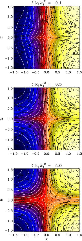
Figure 2: Evolution of the cosmic ray energy density near a magnetic ${\sf X}$-point: snapshots of $e_{\rm c}$ (shown as contours and shades of grey/colour) for field-aligned diffusion along a fixed magnetic field ${\bm{B}}=(\sin k_{1}x,-\sin k_{1}y,0)^{T}$ (shown as vectors) displayed for three times indicated at the top of each frame.

We test the field-aligned diffusion procedure by simulating in two dimensions a magnetic field configuration similar to the X-point discussed in Sect. 2.2. In order to be able to impose normal-field boundary conditions, $\widehat{\mbox{\boldmath$n$}}{}\times{\bm{B}}=0$ at the domain boundaries, we modify the field to ${\bm{B}}=(\sin k_{1}x,-\sin k_{1}y,0)^{T}$, where $k_{1}$ is the smallest wavenumber in a periodic domain. So, for $k_{1}=1$ we consider the domain $-\pi<(x,y)<\pi$. The initial distribution of the cosmic ray energy density is $e_{\rm c}=x$, which has a constant gradient and therefore, with Fickian diffusion, $D_{c}=\mbox{\boldmath$\nabla$}{}\cdot(\widehat{\bm{B}}\widehat{\bm{B}})$ would have a singularity initially. However, in the non-Fickian approach $D_{\rm c}$ is not calculated as in Eq. (9), which resolves this problem. The evolution of $e_{\rm c}$ for $\tau=0.1$ is shown in Fig. 2 together with vectors showing the magnetic field. Note that the gradient of $e_{\rm c}$ becomes small in the neighbourhood of the singularity of $\mbox{\boldmath$\nabla$}{}\cdot(\widehat{\bm{B}}\widehat{\bm{B}})$ at the origin, so the otherwise singular term that multiplies $\mbox{\boldmath$\nabla$}{}e_{\rm c}$ has no effect on $e_{\mathrm{c}}$, as desired. In the case of the Fickian diffusion, the same final solution would have been obtained, but the initial reduction of the gradient in $e_{\mathrm{c}}$ would have involved an infinitely large advection speed ${\bm{U}}_{\rm c}$. In the non-Fickian approach, the maximum propagation speed is $\tilde{K}_{\parallel}^{1/2}$, thereby alleviating the numerical time step problem.

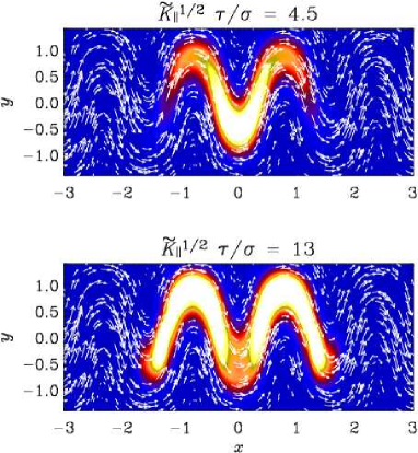
Figure 3: Magnetic field vectors together with a grey/colour scale representation of $e_{\rm c}$ in a kinematic calculation with $128^{2}$ mesh points, for different values of $K_{\parallel}^{1/2}\tau/\sigma$, with $\tilde{K}_{\perp}=0$, $\tilde{K}_{\parallel}=10^{-1}$, and $K_{\rm Fick}=10^{-3}$, at time $t/\tau=1$ for two different values of $\tau$ (=1 and 3, respectively). (Only part of the computational domain in the $y$ direction is shown.)

Another example of field-aligned diffusion is shown in Fig. 3, where the magnetic field is given by ${\bm{B}}={\bm{B}}_{0}+\mbox{\boldmath$\nabla$}{}\times{\bm{A}}$ with ${\bm{B}}_{0}=0.1\widehat{\bm{x}}$ and ${\bm{A}}=0.1\widehat{\bm{z}}\cos(k_{x}x)\cos(k_{y}y)$ with $k_{x}=4k_{1}$ and $k_{y}=k_{1}$. Again, this magnetic field is held constant in time. The initial profile of $e_{\mathrm{c}}\propto\exp(-r^{2}/2\sigma^{2})$, with $r^{2}=x^{2}+(y+0.5)^{2}$, is a two-dimensional Gaussian of a half-width of $\sigma=0.07$, positioned at $(0,-0.5)$. We confirm that our implementation of cosmic ray diffusion allows us to model reliably rather complicated magnetic configurations. The lower panel of Fig. 3 confirms that, for large values of the Strouhal number, the wave nature of the telegraph equation manifests itself and $e_{\mathrm{c}}$ develops two waves propagating away from the initial maximum (similar to the dashed line in Fig. 1).

3 Macroscopic evolution of the cosmic ray gas

3.1 Energy considerations

In a closed domain, mass is conserved, i.e. $\langle\rho\rangle\equiv\rho_{0}=1$, where angular brackets denote volume averaging. Then the hydromagnetic equations coupled with cosmic ray dynamics lead to the following set of equations for the cosmic ray energy $E_{\rm c}=\langle e_{\rm c}\rangle$, the gas energy $E_{\rm g}=\langle e_{\rm g}\rangle$, the kinetic energy $E_{\rm k}=\langle{\textstyle{1\over 2}}\rho{\bm{u}}^{2}\rangle$, and magnetic energy $E_{\rm m}=\langle{\bm{B}}^{2}\rangle/2\mu_{0}$,

$${{\rm d}{}E_{\rm c}\over{\rm d}{}t}=-W_{\rm c}+\langle Q_{\rm c}\rangle,$$ (15)

$${{\rm d}{}E_{\rm g}\over{\rm d}{}t}=-W_{\rm g}+\langle Q_{\rm k}\rangle+\langle Q_{\rm m}\rangle,$$ (16)

$${{\rm d}{}E_{\rm k}\over{\rm d}{}t}=W_{\rm c}+W_{\rm g}+W_{\rm m}+W_{\rm f}-\langle Q_{\rm k}\rangle,$$ (17)

$${{\rm d}{}E_{\rm m}\over{\rm d}{}t}=-W_{\rm m}-\langle Q_{\rm m}\rangle.$$ (18)

Here, all the energies are referred to the unit volume. The terms $W_{\rm c}=\langle p_{\rm c}\mbox{\boldmath$\nabla$}{}\cdot{\bm{u}}\rangle$, $W_{\rm g}=\langle p_{\rm g}\mbox{\boldmath$\nabla$}{}\cdot{\bm{u}}\rangle$, $W_{\rm m}=\langle{\bm{u}}\cdot({\bm{J}}\times{\bm{B}})\rangle$, and $W_{\rm f}=\langle{\bm{u}}\cdot\mbox{\boldmath$f$}{}\rangle$ result from work done against cosmic ray pressure, gas pressure, the Lorentz force, and the external forcing, respectively. Terms responsible for viscous and Joule heating and the cosmic ray energy source are simply given by the volume integrated terms in the original equations. Equations (15)–(18) imply that the total energy, $E_{\rm tot}=E_{\rm c}+E_{\rm g}+E_{\rm k}+E_{\rm m}$, satisfies the simple conservation law

$${{\rm d}{}E_{\rm tot}\over{\rm d}{}t}=\langle Q_{\rm c}\rangle+W_{\rm f}.$$ (19)

Thus, the only sources of energy are the injection of cosmic rays and the external forcing of the turbulence. In the following section we demonstrate how $E_{\rm c}$ can be enhanced by the conversion of kinetic energy.

3.2 Compressional enhancement of cosmic ray energy

We assume $Q_{\rm c}=W_{\rm f}=0$ and that there is initially kinetic energy that is later redistributed among gas and cosmic rays. We investigate, using a simple one-dimensional model ($\partial/\partial y=\partial/\partial z=0$), how much energy can be converted into cosmic ray energy via the $W_{\rm c}$ term responsible for work done against cosmic ray pressure. As the initial condition, we use a sinusoidal perturbation of $u_{x}$ and $\ln\rho$ with unit amplitude and $E_{\rm c}=E_{\rm c0}=1$, $E_{\rm g}=1.8$, and $E_{\rm k}=0.21$. The evolution of velocity, cosmic ray and gas energies, as well as the entropy of the gas are shown in Fig. 4. Here the entropy $s$ is defined as $s=c_{v}\ln(c_{\rm s}^{2}/\rho_{\rm g}^{\gamma-1})$, where $c_{\rm s}^{2}=\gamma(\gamma-1)e_{\rm g}$ is the gas sound speed squared. It turns out that in this case about 78% of the kinetic energy is transformed into cosmic ray energy and only 22% into thermal energy. This result is however sensitive to the phase shift between density and velocity: if the density is initially uniform (keeping all other parameters unchanged), the fractional energy going into cosmic rays is only 23% and 77% go into thermal energy.

Figure 4: Velocity, cosmic ray and gas energy densities, and entropy in an experiment with a non-linear sound wave that piles up to a shock ($\gamma_{\rm c}=5/3$). Note the significant conversion of kinetic energy into cosmic ray energy. The conversion into gas energy is comparatively small even though there is noticeable entropy enhancement due to the shock. Curves obtained for different times are shown with different line types as labelled in the first panel. Time is given in units of $k_{1}^{-1}(E_{\rm c0}/\rho_{0})^{-1/2}$.

These results demonstrate that, at least in principle, a sizable fraction of the kinetic energy can be converted into cosmic ray energy. Similar experiments have been made in earlier work with a similar model in the context of shock acceleration of cosmic rays (see, e.g., Drury & Völk, 1981; Jun et al., 1994). In particular Kang & Jones (1990) showed that the efficiency of conversion varies strongly with $\gamma_{\rm c}$. However, the conversion of kinetic energy into cosmic ray energy requires a background of cosmic ray energy. Decreasing $E_{\rm c}$ from 1 to 0.1 lowers the fraction of compressionally produced cosmic ray energy density from 78% to 21%. In contrast to dynamo theory where a weak seed magnetic field is sufficient to produce equipartition magnetic fields (albeit only in three dimensions), there is no such mechanism for the cosmic ray energy. This is related to the anti-dynamo theorem for scalar fields (Krause, 1972). However, for three-dimensional compressible flows an exponential dynamo-like amplification of a passive scalar is in principle possible if the passive scalar is represented by inertial particles (Elperin et al., 1996). Such a mechanism can work because inertial particles do not feel a pressure gradient. This can lead to particle accumulation in temperature minima (Elperin et al., 1997) and in vortices (Barge & Sommeria, 1995; Hodgson & Brandenburg, 1998; Johansen et al., 2004). However, in this paper cosmic ray particles are treated as non-inertial particles.

3.3 Effect of cosmic ray pressure

Cosmic rays can be confined at large scales by magnetic tension, where a strong magnetic field can more easily withstand deformation driven by cosmic ray pressure gradients. This could provide a natural mechanism for producing equipartition between cosmic rays and the magnetic field. This feature can be simulated in two dimensions in a doubly periodic domain $-\pi<(x,y)<\pi$, with $k_{1}=1$. The results are illustrated in Fig. 5, where we have a magnetic tube in $1<y<2$ with its axis along the $x$ direction. We have implemented two local cosmic ray sources with energy injection profiles

$$Q_{\rm c}=Q_{\rm c0}\sum_{i=1}^{2}\exp\left\{-{\textstyle{1\over 2}}\left[x^{2}+(y-y_{i})^{2}\right]/R^{2}\right\},$$ (20)

i.e., both located on the $y$ axis, centred at $y_{1}=0$ and $y_{2}=\pi/2$; the initial half-widths for both sources is $R=0.13$, so that one source is within the magnetic tube and the other, outside it. In this experiment, cosmic ray diffusion is negligible ($\tilde{K}_{\parallel}=\tilde{K}_{\perp}=0$ and $K_{\rm Fick}=0.01$) as we intend to explore the effects of cosmic ray pressure alone. As expected, expansion proceeds nearly isotropically outside the magnetic structure, but the cosmic ray energy density is channelled preferentially along field lines inside the tube. At the end of the run, the aspect ratio of the cosmic ray distribution is about two to one inside the tube. For values of $Q_{\rm c}$ significantly larger than about 10, the gas density decreases strongly so as to maintain pressure equilibrium and oppose expansion driven by cosmic rays.

This confirms that cosmic ray dynamics can be strongly affected by the approximate pressure balance in the ISM.

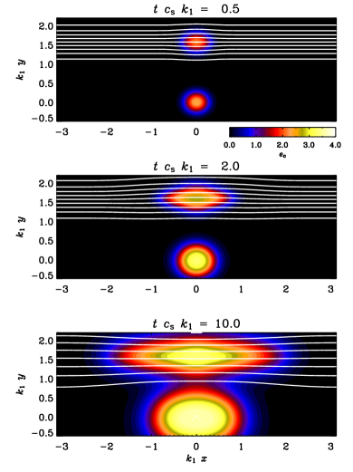
Figure 5: Cosmic ray energy density at times indicated at the top of each panel. Cosmic rays expand from two sources (with injection rate $Q_{\rm c}=10$ for each), one inside a magnetic flux tube and the other one outside. Magnetic lines are shown with white solid curves whose density is proportional to the field strength.

3.4 Cosmic rays in a partially ordered magnetic field

In this section we briefly explore the effects of a random magnetic field on the evolution of the cosmic ray gas. A random component of the interstellar magnetic field can facilitate the isotropic spreading of cosmic rays across the large-scale, preferentially horizontal magnetic field in the Galactic disc. In addition, a turbulent magnetic field can enhance cosmic ray diffusion by destroying the compound diffusion effect (Ptuskin, 1979; Kóta & Jokipii, 2000, and references therein) due to the exponential local divergence of magnetic lines.

To allow for cosmic ray losses through the $x$ boundaries, we relax the assumption of periodicity in that direction. At $x=\pm\pi$, we assume $e_{\rm c}=0$, together with $\partial\rho/\partial x=\partial e_{\rm g}/\partial x=0$. This implies that cosmic rays may be lost from the domain but gas may not. In the $y$ direction we again use periodic boundary conditions.

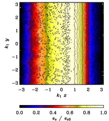
Figure 6: Cosmic ray energy density (colour/grey scale coded, with darker/blue shades corresponding to smaller values) together with magnetic field lines (solid) in a two-dimensional simulation with a fixed magnetic flux tube centred around $x=1.5$ and a random magnetic field superimposed on it. Here, $\tilde{K}_{\parallel}=0.1$, $\tilde{K}_{\perp}=0$, and $\tau=3$.

Figure 7: Cosmic ray energy density from the model of Fig. 6 averaged in the $y$ direction for times $125\times 2^{n}$ with $n=0,...,4$. The magnetic tube is located at $x=1.5$ leading to an asymmetric distribution of cosmic ray energy density.

We consider a two-dimensional system with a regular magnetic field ${\bm{B}}_{0}$ directed along the $y$-axis and confined to a flux tube as shown in Fig. 6, where the field strength has a profile $B_{0}\propto\mbox{sech}^{2}[(x-1.5)/0.5]$. An isotropic random magnetic field $\delta{\bm{B}}$ is superimposed on ${\bm{B}}_{0}$, with $\overline{\delta B^{2}}/B_{0}^{2}=1$ at $x=1.5$ where $B_{0}$ is maximum; the magnetic field does not evolve. The random magnetic field is implemented in terms of a magnetic vector potential given as white noise with Gaussian probability density which, because of two dimensions, implies a $k^{3}$ power spectrum for the magnetic energy. We also assume zero velocity for all times, so we just advance Eqs (2) and (11) in time, using Eq. (6). Cosmic rays are injected at a constant rate across the domain, $Q_{\mathrm{c}}=\mathrm{const}$.

In Fig. 6 we show the result of such a calculation with $\tilde{K}_{\perp}=0$ ; the distribution of cosmic rays in $x$ is asymmetric reflecting the asymmetry in the relative amount of disorder of the magnetic field, $\overline{\delta B^{2}}/B_{0}^{2}$. This asymmetry can be seen more clearly in Fig. 7 which shows the evolution of cosmic ray energy density averaged in the $y$-direction. (Note however that the steady state is only attained after very long times. Here, $t=2000$ corresponds to $t\tau\tilde{K}_{\parallel}k_{1}^{2}=600$.)

The effective perpendicular diffusivity due to the randomness of the magnetic field, $K_{\perp}^{\mathrm{(eff)}}(x)$, can be obtained from the steady-state equation

$${{\rm d}{}\over{\rm d}{}x}\left(K_{\perp}^{\mathrm{(eff)}}(x){{\rm d}{}e_{\mathrm{c}}\over{\rm d}{}x}\right)=-Q_{\mathrm{c}},$$ (21)

which can be integrated to obtain

$$K_{\perp}^{\mathrm{(eff)}}(x)=(x_{0}-x)Q_{\mathrm{c}}\left({{\rm d}{}e_{\rm c}\over{\rm d}{}x}\right)^{-1},$$ (22)

where $x_{0}$ is the position where ${\rm d}{}e_{\mathrm{c}}/{\rm d}{}x=0$. The resulting profile of $K_{\perp}^{\mathrm{(eff)}}$, shown in Fig. 8 along with

$$\chi=\frac{\overline{\delta B^{2}}}{B_{0}^{2}+{\textstyle{1\over 3}}\delta B^{2}}=3\,\frac{\overline{B_{x}^{2}}}{\overline{B_{y}^{2}}},$$ (23)

confirms that the effective perpendicular diffusion is controlled by the degree of randomness of the magnetic field (see, e.g., Chuvilgin & Ptuskin, 1993).

Figure 8: The profile of $K_{\perp}^{\mathrm{(eff)}}$ (solid) obtained from Eq. (22) using $e_{\rm c}$ corresponding to the upper curve of Fig. 7, and $\chi=3\overline{B_{x}^{2}}/\overline{B_{y}^{2}}$ (dashed), where $B_{y}$ has both large-scale and random parts, whereas $B_{x}$ is a purely random magnetic field. Here, $K_{\mathrm{max}}=0.023$ is the maximum value of $K_{\perp}^{\mathrm{(eff)}}$.

4 Cosmic rays in a magnetic field produced by dynamo action

Three-dimensional turbulence is capable of dynamo action for sufficiently large magnetic Reynolds numbers, and the dynamo-generated magnetic field organizes itself into random flux tubes or sheets (e.g. Zeldovich et al., 1990; Brandenburg et al., 1995; Brandenburg & Subramanian, 2005, and references therein). Most studies of cosmic ray dynamics neglect the specific features of the magnetic fields produced by turbulent dynamos. We provide here a preliminary discussion of cosmic ray evolution in a magnetic field generated by a turbulent flow of electrically conducting fluid. The magnetic field structure of these simulations is realistic enough to include important physical effects such as the enhancement of cosmic ray diffusion by turbulent fields, as mentioned in Sect. 3.4.

Magnetic field produced by the dynamo action is rather different from that prescribed as, say, a random vector field with given spectrum and Gaussian statistical properties of the components. In contrast to such ad hoc models, dynamo magnetic fields can be strongly intermittent (i.e., dominated by intense magnetic filaments, ribbons and sheets) and varying in time (see Brandenburg & Subramanian, 2005, and references therein); both features can affect the propagation of charged particles. Moreover, since both gas flow and magnetic field are random (in space and time), any relation between cosmic ray energy density and other parameters of the medium (e.g., magnetic energy density or gas density) can only be statistical. Therefore, we expect that the energy density of cosmic rays can locally (and at any given moment) significantly exceed, say, the magnetic energy density. However, one would expect that some form of equipartition between energy densities (or forces due to) cosmic rays and magnetic fields can be maintained on average. We note, however, that simulations have not fully confirmed these expectations; see also Padoan & Scalo (2005).

Our model is realistic with respect to modelling fully nonlinear dynamo action as we simulate consistently both a randomly forced flow and the magnetic field produced by it, by solving both the Navier–Stokes and induction equations (with the Lorentz force included in the former, and the velocity field obtained from the Navier–Stokes equation in the latter). The turbulent motions in our model are driven by a random force explicitly included in the Navier–Stokes equation. In reality, interstellar turbulence is driven by supernova explosions that produce strongly compressible flows with very large local Mach numbers locally (some aspects of the relevant models are reviewed by Mac Low & Klessen, 2004). However, we deliberately restrain ourselves from a detailed discussion of such more realistic models here (which would also include stratification, disc–halo connections, velocity shear, etc.), but instead explore just the effects of magnetic intermittency and variability. We believe that our simulations capture at least some of the most important effects of interstellar dynamo action on the cosmic ray propagation (within the limits of our model for the cosmic rays).

The turbulence in our simulations is driven helically by a forcing function $f$ in the Navier–Stokes equation, as was done in the simulations of Brandenburg (2001), for example. At $x=\pm\pi$, we use stress-free normal field boundary conditions (as was also done in Brandenburg & Dobler, 2001), and assume $e_{\rm c}=0$ on the boundaries as in Sect. 3.4. In the other directions we take periodic boundary conditions. Our analysis of the results presented below only uses positions that are some distance away from the domain boundaries ($L_{x}/8$ on both boundaries) to reduce their influence. (Including boundary points merely tends to decrease the magnitude of the correlation coefficients between the various energy densities, but it does not change the results qualitatively.) The forcing function is given in Appendix B and its (dimensionless) amplitude for the simulation shown here is chosen to be $f_{0}=2$, which produces an rms Mach number of about 1.2.

The forcing wavenumber is chosen to be $k_{\rm f}=1.5\,k_{1}$. This value is close to the wavenumber corresponding to the box size, $k_{1}=2\pi/L_{x}$, so we do not expect to have clearly distinct large-scale and small-scale magnetic fields. Generally, the flow helicity allows us to obtain dynamo action at relatively small values of the magnetic Reynolds number defined as $R_{\rm m}=u_{\rm rms}/(\eta k_{\rm f})$. However, because of the non-periodic boundaries in the $x$ direction, and also because of the weak scale separation ($k_{\rm f}/k_{1}$ is not very large), the critical value of $R_{\rm m}$ with respect to the onset of dynamo action is still around ${R_{\mathrm{m}}}_{\mathrm{,cr}}=30$, which is similar to what would be expected for a non-helical random flow in a periodic domain. The simulation presented here has $R_{\rm m}\approx 150$. The kinematic growth rate of the rms magnetic field is about $0.06\,u_{\rm rms}k_{\rm f}$. In Fig. 9 we show the evolution of the magnetic energy together with kinetic and cosmic ray energies. We see that the magnetic field grows exponentially for $t\mathrel{\mathchoice{\vbox{\offinterlineskip\halign{\hfil$\displaystyle#$\hfil\cr<\cr\sim\cr}}}{\vbox{\offinterlineskip\halign{\hfil$\textstyle#$\hfil\cr<\cr\sim\cr}}}{\vbox{\offinterlineskip\halign{\hfil$\scriptstyle#$\hfil\cr<\cr\sim\cr}}}{\vbox{\offinterlineskip\halign{\hfil$\scriptscriptstyle#$\hfil\cr<\cr\sim\cr}}}}150/(u_{\rm rms}k_{\rm f})$ and then saturates—in agreement with earlier simulations quoted above. We note that the energy density of cosmic rays is much larger than magnetic energy density at these early times; nevertheless, the cosmic ray energy increases rather slowly after $t\mathrel{\mathchoice{\vbox{\offinterlineskip\halign{\hfil$\displaystyle#$\hfil\cr>\cr\sim\cr}}}{\vbox{\offinterlineskip\halign{\hfil$\textstyle#$\hfil\cr>\cr\sim\cr}}}{\vbox{\offinterlineskip\halign{\hfil$\scriptstyle#$\hfil\cr>\cr\sim\cr}}}{\vbox{\offinterlineskip\halign{\hfil$\scriptscriptstyle#$\hfil\cr>\cr\sim\cr}}}}50/(u_{\rm rms}k_{\rm f})$. The steady-state energy density of cosmic rays is controlled by their injection rate $Q_{\mathrm{c}}$ and their diffusivity: solutions of Eq. (21) are proportional to $Q_{\mathrm{c}}/K^{(\rm eff)}_{\perp}$. However, the effective diffusivity of cosmic rays is controlled by the degree of tangling of the magnetic field rather than by the field strength itself; see, e.g., Eq. (23). It is not surprising, then, that even a weak magnetic field can confine cosmic rays at early times in this model. The linear dependence of the steady-state energy density of cosmic rays on their injection rate is a direct consequence of the (almost) linear nature of the cosmic ray dynamics as described by Eq. (2); the only nonlinearity here is that the cosmic ray energy density affects the flow through the pressure term, and then the velocity field enters the induction equation and the advection term for the cosmic rays. However, this nonlinearity is not very strong, and our simulations confirm a linear dependence of $e_{\mathrm{c}}$ on $Q_{\mathrm{c}}$ within a broad range of the latter (at least two orders of magnitude). The magnetic field part $B_{0}$ is understood, in the present context, as an average over a scale smaller than the domain size but larger than, say, the gyro radius of cosmic ray particles.

Figure 9: Time series of magnetic ($E_{\mathrm{m}}$), kinetic ($E_{\mathrm{k}}$) and cosmic ray ($E_{\mathrm{c}}$) energies in a dynamo simulation. Here, time is given in turnover times $(u_{\rm rms}k_{\rm f})^{-1}$, and $e_{\rm c0}=L_{x}^{2}Q_{\rm c}/K_{\parallel}$ is used to normalize energies per unit volume. The thermal energy of the gas is constant with $E_{\rm g}/e_{\rm c0}\approx 0.7$.

For the simulation shown here we have chosen $Q_{\rm c}=0.01$, which yields a steady-state cosmic ray energy of $E_{\rm c}\approx 1$ in units of $L_{x}^{2}Q_{\mathrm{c}}/K_{\parallel}$. The other parameters of the simulation presented here are $\tilde{K}_{\perp}=0$, $\tilde{K}_{\parallel}=0.3$, $K_{\rm Fick}=2\times 10^{-2}$, $\tau=0.3$, $\eta=5\times 10^{-3}$, $\nu=0.5$. Furthermore, because the Mach number is slightly larger than unity, an additional bulk viscosity proportional to the negative velocity divergence has been included. This is usually referred to as a shock viscosity; see Haugen et al. (2004) for details and the definition of a non-dimensional parameter $c_{\rm shock}$ which is here chosen to be 10. The value of $\tilde{K}_{\parallel}$ is chosen to be close to the maximum Alfvén speed squared. The magnetic field produced by the dynamo has pronounced magnetic filaments whose half-width (radius) is about $\ell=0.2$, which is consistent with the estimate $\ell\simeq\pi k_{\mathrm{f}}^{-1}R_{\rm m,cr}^{-1/2}$ suggested by Subramanian (1999). For $\tau=0.3$ and $\ell=0.2$, we have $\mbox{St}\approx 1$ from Eq. (13). The steady-state mean kinetic energy density depends directly on the intensity of the forcing. On the other hand, the ratio of magnetic to kinetic energy densities is controlled by the nature of the dynamo action. The above parameter values have been chosen as to ensure that the energy densities of magnetic field and cosmic rays are of the same order of magnitude in the statistically steady state.

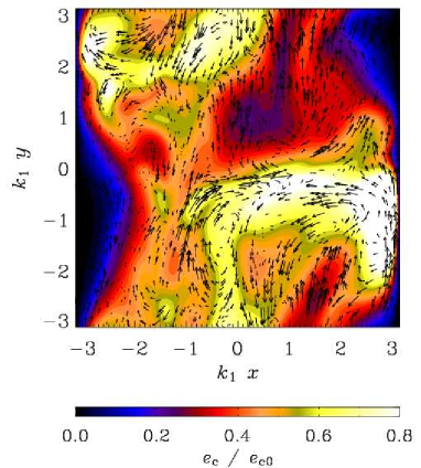
Figure 10: Cosmic ray energy density (colour/grey-scale coded, with lighter shades/redder colour corresponding to larger values) and magnetic field vectors in a slice taken from a dynamo simulation. The magnetic field vectors are more numerous where magnetic field strength is larger.

In Fig. 10 we show a typical cross-section of the cosmic ray energy density and magnetic field vectors from the three-dimensional dynamo simulation of Fig. 9 at $t=250/(u_{\rm rms}k_{\rm f})$. The cosmic ray energy density declines toward the boundaries at $x=\pm\pi$, where the boundary condition $e_{\mathrm{c}}=0$ is imposed, and shows some moderate variation inside the domain. There is no pronounced correlation with magnetic field strength even though imprints of the field-aligned diffusion can clearly be seen, e.g., between $(x,y)k_{1}=(-1,-1)$ and $(0,0)$. We show in Fig. 11 a two-dimensional joint probability density function of $\log B^{2}$ and $e_{\mathrm{c}}$ (normalized to unit integral as usual), which demonstrates the lack of any noticeable correlation between these variables. The finite lifetime of magnetic structures produced by the dynamo must be one of the reasons of the lack of correlation between the two variables. There is some correlation between gas density and cosmic ray energy density, as shown in Fig. 12, but the cross-correlation coefficient is only 0.54, with the best-fitting dependence $e_{\mathrm{c}}/e_{\mathrm{c0}}\simeq\rho/\rho_{0}$.

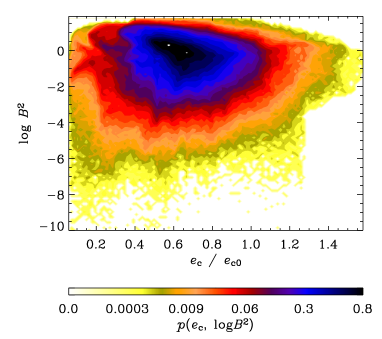
Figure 11: Two-dimensional histogram (or joint probability density) of magnetic pressure and cosmic ray energy density. Here, $e_{\rm c0}=L_{x}^{2}Q_{\rm c}/K_{\parallel}$ is used to normalize $e_{\rm c}$. The two-dimensional probability density is calculated using only points at a distance greater than $L_{x}/8$ from the boundaries in an attempt to avoid the regions where the distribution of $e_{\mathrm{c}}$ is affected by the boundary conditions.

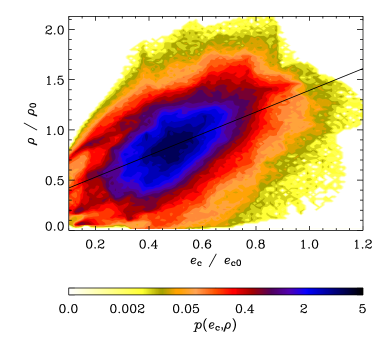
Figure 12: As in Fig. 11, but for gas density and cosmic ray energy density, showing a modest correlation between the two. The correlation coefficient is $r=0.54$, and the straight line is a best-fitting line.

If the injection rate of cosmic rays is reduced by a factor of ten to $Q_{\mathrm{c}}=10^{-3}$, the resulting steady-state mean value of the cosmic ray energy density is found to be reduced by about the same factor. The relation between cosmic ray energy density and gas density still appears to be nearly linear, but the cross-correlation coefficient is now larger, varying with time in the range 0.7–1.

We have also explored a run with a Mach number of 0.2 (achieved by using a weaker driving force; $f_{0}=0.05$) but with the same injection rate of cosmic rays as above, $Q_{\mathrm{c}}=0.01$. The resulting steady-state mean energy density of cosmic rays exceeds those of magnetic field and turbulence, $E_{\mathrm{c}}/e_{\mathrm{c0}}\simeq 1$, $E_{\mathrm{k}}/e_{\mathrm{c0}}\simeq 0.02$ and $E_{\mathrm{m}}/e_{\mathrm{c0}}\simeq 0.01$. This produces significant anticorrelation between cosmic ray energy density and gas density (cross-correlation coefficient of $-0.94$), with a linear dependence between $e_{\mathrm{c}}$ and $\rho$.

The latter anticorrelation may be attributed to the average pressure equilibrium in the domain, while a positive correlation in the supersonic flow may arise as both gas and cosmic rays are compressed by the gas flow. We have confirmed that no positive correlation between cosmic rays and gas density occurs if the cosmic ray advection is neglected.

The model illustrated in Figs 9 and 10 is close to energy equipartition between cosmic rays, magnetic field and turbulence. We note however that the Lorentz force and the cosmic ray pressure gradient have very different magnitudes because the field-aligned cosmic ray diffusivity is much larger than the magnetic diffusivity. As a result, the cosmic rays are distributed more uniformly than the magnetic field and the gas density and so the cosmic ray pressure gradient is comparatively small. For the values of the diffusivities given above, the ratio the rms cosmic ray pressure gradient, $F_{\mathrm{c}}$, and the rms Lorentz force $F_{\mathrm{m}}$, is typically about $0.1$ of the ratio of the corresponding mean energy densities; this also applies if the Lorentz force is replaced by the gradient of kinetic energy density. The typical length scale of the magnetic field is about $\ell\simeq l_{0}R_{\mathrm{m,cr}}^{-1/2}$ and $F_{\mathrm{m}}\simeq e_{\mathrm{m}}/\ell$, with $l_{0}\simeq 100\,{\rm pc}$ the turbulent scale and ${R_{\mathrm{m}}}_{\mathrm{,cr}}\approx 30$ the critical magnetic Reynolds number for the onset of dynamo action (see above). The length scale of the cosmic ray distribution can be estimated as the diffusion scale over the confinement time $\tau_{\mathrm{c}}\simeq 10^{7}\,{\rm yr}$, $l_{\mathrm{c}}\simeq(K_{\parallel}\tau_{\mathrm{c}})^{1/2}$. Then, for $K_{\parallel}=10^{28}\,{\rm cm}^{2}\,{\rm s}^{-1}$,

$$\frac{F_{\mathrm{c}}}{F_{\mathrm{m}}}\simeq\frac{\ell}{l_{\mathrm{c}}}\,\frac{E_{\mathrm{c}}}{E_{\mathrm{m}}}\simeq\frac{1}{30}\,\frac{E_{\mathrm{c}}}{E_{\mathrm{m}}}\;.$$

This conclusion appears to be model-independent and suggests that energy equipartition between cosmic rays and other constituents of the interstellar medium does not necessarily imply that cosmic rays play an important role in the dynamical balance.

5 Discussion and conclusions

We have presented a preliminary analysis of cosmic ray propagation in a magnetic field produced by dynamo action of a turbulent flow. The confinement of cosmic rays resulting from their scattering by magnetohydrodynamic waves can be modelled with an equation similar to Eq. (2), where the advection velocity is a linear combination of gas velocity and Alfvén velocity (Skilling, 1975). Our results are based on advection with the local gas velocity. Padoan & Scalo (2005) considered local variations in cosmic ray density in the case where the advection velocity is given by the Alfvén velocity. They predict that $e_{\mathrm{c}}\propto n_{\mathrm{i}}^{1/2}$, with $n_{\mathrm{i}}$ the ion density. This scaling is expected if the diffusive streaming velocity, $-K_{\parallel}\nabla e_{\mathrm{c}}$, and the effects of cosmic ray pressure are negligible. Our model can be adapted to test and generalize these results; the anticorrelation between $e_{\mathrm{c}}$ and gas density in one of our models (with low Mach number) seems to be a direct consequence of pressure balance, while a positive correlation (obtained at larger Mach number) may reflect the fact that both cosmic rays and thermal gas experience similar compression by the gas flow. We have shown that our model captures naturally the dependence of the effective diffusivity of cosmic rays on the ratio of random to ordered magnetic field, $\delta B^{2}/B_{0}^{2}$.

The diffusivity of cosmic rays along the magnetic field is rather large; the corresponding Strouhal number, defined in Eq. (13) may significantly exceed unity, as shown in Eq. (14). For comparison, a similar estimate yields $\mathrm{St}\simeq 1$ for the turbulent kinetic and magnetic diffusivities in the ISM. This motivates our suggestion that the standard Fickian diffusion model, which leads to the classical diffusion equation, may be a poor approximation for cosmic rays, and a more accurate description leading to some form of the telegraph equation might be more appropriate. Formally, the difference between the two approximations consists of retaining, in the latter approximation, higher-order terms in the correlation time of the random process underlying diffusion. We have introduced this effect to alleviate numerical problems, but it can be a real physical effect which deserves further careful study.

In summary, we have found that the cosmic ray distribution can be more uniform than the distributions of magnetic field and gas density. Consequently, we may argue that energy equipartition between cosmic rays and other constituents of the interstellar medium does not necessarily imply that cosmic rays play a significant role in the dynamical balance.

Appendix A Boundedness of cosmic ray energy density

In this section we show that, in a closed or periodic domain, $\max(e_{\rm c})$ can only decrease as a result of (tensorial) diffusion. This is useful for showing that the diverging behaviour of $U_{\rm c}$ does not produce a singularity in $e_{\rm c}$; cf. Sect. 2.2. In order to avoid interference from other effects, we assume that the evolution of $e_{\rm c}$ is only governed by diffusion, i.e.

$${\partial e_{\rm c}\over\partial t}=\nabla_{i}\left(K_{ij}\nabla_{j}e_{\rm c}\right).$$ (24)

Note also that $\max(e_{\rm c})=\langle e_{\rm c}^{n}\rangle^{1/n}$ for $n\to\infty$. Here, angular brackets denote volume averages. Thus, using integration by parts, we have

$${{\rm d}{}\over{\rm d}{}t}\langle e_{\rm c}^{n}\rangle = n\left\langle e_{\rm c}^{n-1}{\partial e_{\rm c}\over\partial t}\right\rangle=n\left\langle e_{\rm c}^{n-1}\nabla_{i}\left(K_{ij}\nabla_{j}\right)\right\rangle$$ (25)

$$= -n(n-1)\left\langle e_{\rm c}^{n-2}K_{ij}(\nabla_{i}e_{\rm c})(\nabla_{j}e_{\rm c})\right\rangle$$

$$\leq 0\quad\mbox{(for any value of $n>1$)}.$$

The last inequality assumes that the diffusion tensor is positive definite, which is true in our case, because

$$K_{ij}(\nabla_{i}e_{\rm c})(\nabla_{j}e_{\rm c})\!=\!(K_{\parallel}\!-\!K_{\perp})(\widehat{\bm{B}}\cdot\mbox{\boldmath$\nabla$}{}e_{\rm c})^{2}\!+\!K_{\perp}(\mbox{\boldmath$\nabla$}{}e_{\rm c})^{2}$$ (26)

is positive. Therefore, $\max(e_{\rm c})$ must decrease with time.

Appendix B The forcing function

For completeness we specify here the forcing function used in the present paper. It is defined as

$$\mbox{\boldmath$f$}{}({\bm{x}},t)={\rm Re}\{N\mbox{\boldmath$f$}{}_{{\bm{k}}(t)}\exp[{\rm i}{\bm{k}}(t)\cdot{\bm{x}}+{\rm i}\phi(t)]\},$$ (27)

where ${\bm{x}}$ is the position vector. The wavevector ${\bm{k}}(t)$ and the random phase $-\pi<\phi(t)\leq\pi$ change at every time step, so $\mbox{\boldmath$f$}{}({\bm{x}},t)$ is $\delta$-correlated in time. For the time-integrated forcing function to be independent of the length of the time step $\delta t$, the normalization factor $N$ has to be proportional to $\delta t^{-1/2}$. On dimensional grounds it is chosen to be $N=f_{0}\rho_{0}c_{\rm s}(|{\bm{k}}|c_{\rm s}/\delta t)^{1/2}$, where $f_{0}$ is a dimensionless forcing amplitude. At each time step we select randomly one of many possible wavevectors in a certain range around a given forcing wavenumber. The average wavenumber is referred to as $k_{\rm f}$. Two different wavenumber intervals are considered: $1$–$2$ for $k_{\rm f}=1.5$ and $4.5$–$5.5$ for $k_{\rm f}=5$. We force the system with transverse helical waves,

$$\mbox{\boldmath$f$}{}_{{\bm{k}}}=\mbox{\boldmath$\sf R$}{}\cdot\mbox{\boldmath$f$}{}_{{\bm{k}}}^{\rm(nohel)}\quad\mbox{with}\quad{\sf R}_{ij}={\delta_{ij}-{\rm i}\sigma\epsilon_{ijk}\hat{k}_{k}\over\sqrt{1+\sigma^{2}}},$$ (28)

where $\sigma=1$ for positive helicity of the forcing function,

$$\mbox{\boldmath$f$}{}_{{\bm{k}}}^{\rm(nohel)}=\left({\bm{k}}\times\widehat{\mbox{\boldmath$e$}}{}\right)/\sqrt{{\bm{k}}^{2}-({\bm{k}}\cdot\widehat{\mbox{\boldmath$e$}}{})^{2}},$$ (29)

is a non-helical forcing function, and $\widehat{\mbox{\boldmath$e$}}{}$ is an arbitrary unit vector not aligned with ${\bm{k}}$; note that $|\mbox{\boldmath$f$}{}_{{\bm{k}}}|^{2}=1$.

References

- Bakunin (2003a) Bakunin, O. G. 2003a, Uspekhi Fiz. Nauk, 173, 317 (Physics-Uspekhi, 46, 309)
- Bakunin (2003b) Bakunin, O. G. 2003b, Uspekhi Fiz. Nauk, 173, 757 (Physics-Uspekhi, 46, 733)
- Berezinskii et al. (1990) Berezinskii, V. S., Bulanov, S. V., Dogiel, V. A., Ginzburg, V. L., & Ptuskin, V. S. 1990, Astrophysics of Cosmic Rays (V. L. Ginzburg, ed.), Amsterdam, North-Holland
- Blackman & Field (2003) Blackman, E. G., & Field, G. B. 2003, Phys. Fluids, 15, L73
- Barge & Sommeria (1995) Barge, P., & Sommeria, J. 1995, A&A, 295, L1
- Brandenburg (2001) Brandenburg, A. 2001, ApJ, 550, 824
- Brandenburg & Dobler (2001) Brandenburg, A., & Dobler, W. 2001, A&A, 369, 329
- Brandenburg & Subramanian (2005) Brandenburg, A., & Subramanian, K. 2005, Phys. Rep., 417, 1
- Brandenburg et al. (1995) Brandenburg, A., Procaccia, I., & Segel, D. 1995, Phys. Plasmas, 2, 1148
- Brandenburg et al. (2004) Brandenburg, A., Käpylä, P., & Mohammed, A. 2004, Phys. Fluids, 16, 1020
- Cesarsky (1980) Cesarsky, C. J. 1980, ARA&A, 18, 289
- Chuvilgin & Ptuskin (1993) Chuvilgin, L. G., & Ptuskin, V. S., 1993, A&A, 279, 278
- Drury & Völk (1981) Drury, L. O’C., & Völk, J. H. 1981, ApJ, 248, 344
- Elperin et al. (1996) Elperin, T., Kleeorin, N., & Rogachevskii, I. 1996, Phys. Rev. Lett., 77, 5373
- Elperin et al. (1997) Elperin, T., Kleeorin, N., & Rogachevskii, I. 1997, Phys. Rev. E, 55, 2713
- Farmer & Goldreich (2004) Farmer, A. J., & Goldreich, P. 2004, ApJ, 604, 671
- Felice & Kulsrud (2001) Felice, G. M., & Kulsrud, R. M. 2001, ApJ, 553, 198
- Gombosi et al. (1993) Gombosi, T. I., Jokipii, J. R., Kota, J., Lorencz, K., & Williams, L. L. 1993, ApJ, 403, 377
- Hanasz & Lesch (2003) Hanasz, M. & Lesch, H. 2003, A&A, 412, 331
- Hanasz et al. (2004) Hanasz, M., Kowal, G., Otmianowska-Mazur, K., & Lesch, H. 2004, ApJ, 605, L33
- Haugen et al. (2004) Haugen, N. E. L., Brandenburg, A., & Mee, A. J. 2004, MNRAS, 353, 947
- Hillas (2005) Hillas, A. M. 2005, J. Phys. G: Nucl. Part. Phys., 31, R95
- Hodgson & Brandenburg (1998) Hodgson, L. S. & Brandenburg, A. 1998, A&A, 330, 1169
- Johansen et al. (2004) Johansen, A., Andersen, A. C., & Brandenburg, A. 2004, A&A, 417, 361
- Jun et al. (1994) Jun, B.-I., Clarke, D. A., & Norman, M. L. 1994, ApJ, 429, 748
- Kang & Jones (1990) Kang, H., & Jones, T. W. 1990, ApJ, 353, 149
- Kóta & Jokipii (2000) Kóta, F., & Jokipii, J. R. 2000, ApJ, 531, 1067
- Krause (1972) Krause, F. 1972, AN, 294, 83
- Krause & Rädler (1980) Krause, F., & Rädler, K.-H. 1980, Mean-Field Magnetohydrodynamics and Dynamo Theory (Akademie-Verlag, Berlin; also Pergamon Press, Oxford)
- Landau & Lifshitz (1987) Landau, L. D., & Lifshitz, E. M. 1987, Fluid Mechanics (2nd Edition, Pergamon Press, Oxford)
- Mac Low & Klessen (2004) Mac Low, M.-M., & Klessen, R. S., 2004, Rev. Mod. Phys., 76, 125
- Miller & Stone (2000) Miller, K. A. & Stone, J. M. 2000, ApJ, 534, 398
- Moss et al. (1999) Moss, D., Shukurov, A., & Sokoloff, D. 1999, A&A, 343, 120
- Padoan & Scalo (2005) Padoan, P., & Scalo, J. 2005, ApJ, 624, L97
- Parker (1966) Parker, E. N. 1966, ApJ, 145, 811
- Parker (1992) Parker, E. N. 1992, ApJ, 401, 137
- Ptuskin (1979) Ptuskin, V. S. 1979, ApSS, 61, 359
- Ryu et al. (2003) Ryu, D., Kim, J., Hong, S. S., & Jones, T. W. 2003, ApJ, 589, 338
- Schlickeiser & Lerche (1985) Schlickeiser, R., & Lerche, I. 1985, A&A, 151, 151
- Skilling (1975) Skilling, J. 1975, MNRAS, 173, 255
- Subramanian (1999) Subramanian K., 1999, Phys. Rev. Lett., 83, 2957
- Zeldovich et al. (1990) Zeldovich, Ya. B., Ruzmaikin, A. A., & Sokoloff, D. D. 1990, The Almighty Chance (World Scientific, Singapore)