A new constraint on the time dependence of
the proton$-$to$-$electron mass ratio

A new limit on the possible cosmological variation of the proton-to-electron mass ratio $\mu=m_{p}/m_{e}$ is estimated by measuring wavelengths of H₂ lines of Lyman and Werner bands from two absorption systems at $z_{\rm abs}=2.5947$ and $3.0249$ in the spectra of quasars Q 0405$-$443 and Q 0347$-$383, respectively. Data are of the highest spectral resolution ($R$ = 53000) and S/N ratio (30$\div$70) for this kind of study. We search for any correlation between $z_{\rm i}$, the redshift of observed lines, determined using laboratory wavelengths as references, and $K_{\rm i}$, the sensitivity coefficient of the lines to a change of $\mu$, that could be interpreted as a variation of $\mu$ over the corresponding cosmological time. We use two sets of laboratory wavelengths, the first one, Set (A) (Abgrall et al. Abgr (1993)), based on experimental determination of energy levels and the second one, Set (P) (Philip et al. Philip (2004)), based on new laboratory measurements of some individual rest-wavelengths. We find $\Delta\mu$/$\mu$ = (3.05$\pm$0.75)$\times$10^-5 for Set (A), and $\Delta\mu$/$\mu$ = (1.65$\pm$0.74)$\times$10^-5 for Set (P). The second determination is the most stringent limit on the variation of $\mu$ over the last 12 Gyrs ever obtained. The correlation found using Set (A) seems to show that some amount of systematic error is hidden in the determination of energy levels of the H₂ molecule.

1 Introduction

Contemporary theories of fundamental interactions (Strings/M-theory and others) predict some variation of the fundamental physical constants in the course of the evolution of the Universe. Most of the predictions of such theories lie in the energy range inaccessible to current experiments ($E\sim 10^{19}$ GeV). However, at lower energy, variations of the fundamental constants, in principle, could be a possible observational manifestations of these theories. It is therefore important to constrain these variations as a step toward a better understanding of Nature.

A considerable amount of interest in the possibility of time variations of fundamental constants has been generated by recent observations of quasar absorption systems. Using a new method, the so-called Many-Multiplet analysis (Webb et al., Webb1 (1999); Dzuba et al., Dzuba (1999)), Murphy et al. (Murphy03 (2003)) have claimed that the fine structure constant, $\alpha=e^{2}/\hbar c$, could have varied over the redshift range $0.2<z<3.7$ with the amplitude $\Delta\alpha/\alpha=(-0.543\pm 0.116)\times 10^{-5}$. However, a stringent upper limit on the variation of $\alpha$ has been obtained from a large sample of UVES data, $\Delta\alpha/\alpha=(-0.06\pm 0.06)\times 10^{-5}$ over $0.4<z<2.3$ (Srianand et al. 2004, Chand et al. 2004). In addition, Quast et al. (Quast (2004)) derived $\Delta\alpha/\alpha=(-0.04\pm 0.19\pm 0.27)\times 10^{-5}$ from an analysis of one system at $z_{\rm abs}=1.15$.

One way to solve the controversy is to constrain other fundamental constants. Different theoretical models of the fundamental physical interactions predict different variations of their values and different relations between cosmological deviations of the constants ($\alpha$, $\mu$, and others, see Calmet & Fritzsch Calmet (2002), Langacker et al., Langacker (2002), Olive et al. Olive (2002), Dent & Fairbairn Dent (2003)). Therefore, it is crucial to couple measurements of different dimensionless fundamental constants.

2 The proton-to-electron mass ratio $\mu=m_{p}/m_{e}$

Here we use QSO absorption lines to constrain $\,\Delta\mu/\mu$ with $\,\Delta\mu=\mu-\mu_{0}$, where $\,\mu\,$ is the proton-to-electron mass ratio at the epoch of the QSO absorption spectrum formation and $\mu_{0}$ is its contemporary value.

In the framework of unified theories (e.g. SUSY GUT) with a common origin of the gauge fields, variations of the gauge coupling $\alpha_{GUT}$ at the unified scale ($\sim 10^{16}$ GeV) will induce variations of all the gauge couplings in the low energy limit, $\alpha_{i}=f_{i}(\alpha_{GUT},E)$, and provide a relation $\Delta\mu/\mu\simeq R\Delta\alpha/\alpha$, where $R$ is a model dependent parameter and $|R|\;\raise 1.29167pt\hbox{$<$\kern-7.5pt\raise-4.73611pt\hbox{$\sim$}}\;50$ (e.g. Dine et al., Dine (2003) and references therein). Thus, independent estimates of $\Delta\alpha/\alpha$ and $\Delta\mu/\mu$ could constrain the mass formation mechanisms in the context of unified theories.

At present the proton-to-electron mass ratio has been measured with a relative accuracy of $2\times 10^{-9}$ and equals $\mu_{0}=1836.15267261(85)$ (Mohr & Taylor, Mohr (2000)). Laboratory metrological measurements rule out considerable variation of $\mu$ on a short time scale but do not exclude its changes over the cosmological scale, $\sim 10^{10}$ years. Moreover, one can not reject the possibility that $\mu$ (as well as other constants) could be different in widely separated regions of the Universe.

The method used here to constrain the possible variations of $\mu$ was proposed by Varshalovich and Levshakov (VarshLev (1993)). It is based on the fact that wavelengths of electron-vibro-rotational lines depend on the reduced mass of the molecule, with the dependence being different for different transitions. It enables us to distinguish the cosmological redshift of a line from the shift caused by a possible variation of $\mu$.

Thus, the measured wavelength $\lambda_{i}$ of a line formed in the absorption system at the redshift $z_{abs}$ can be written as

$$\lambda_{\rm i}=\lambda_{\rm i}^{0}(1+z_{abs})(1+K_{\rm i}\Delta\mu/\mu)$$ (1)

where $\lambda_{\rm i}^{0}$ is the laboratory (vacuum) wavelength of the transition, and $K_{\rm i}=\mbox{d}\ln\lambda_{\rm i}^{0}/\mbox{d}\ln\mu$ is the sensitivity coefficient calculated for the Lyman and Werner bands of molecular hydrogen in work (Varshalovich and Potekhin, VarshPo (1995)). This expression can be represented in terms of the individual line redshift $z_{\rm i}\equiv\lambda_{\rm i}/\lambda_{\rm i}^{0}-1$ as

$$z_{\rm i}=z_{abs}+bK_{\rm i}$$ (2)

where $b=(1+z_{abs})\Delta\mu/\mu$. Note, in case of nonzero $\Delta\mu/\mu$, $z_{\rm abs}$ is not equal to the standard mean value $\overline{z}=(\Sigma\,z_{\rm i})/N$.

In reality, $z_{\rm i}$ is measured with some uncertainty which is caused by statistical errors of the astronomical measurements $\lambda_{\rm i}$, by errors of the laboratory measurements of $\lambda_{\rm i}^{0}$, and by possible systematic errors. Nevertheless, if $\Delta\mu/\mu$ is nonzero, there must be a correlation between $z_{\rm i}$ and $K_{\rm i}$ values. Thus, a linear regression analysis of these quantities yields $z_{\rm abs}$ and $b$ (as well as their statistical significance), consequently an estimate of $\Delta\mu/\mu$.

Previous studies have already yielded tight upper limits on $\mu$-variations, $|\Delta\mu/\mu|<7\times 10^{-4}$ (Cowie & Songaila, Cowie (1995)), $|\Delta\mu/\mu|<2\times 10^{-4}$ (Potekhin et al., PIV (1998)), $|\Delta\mu/\mu|<5.7\times 10^{-5}$ (Levshakov et al., 2002a ), and $\Delta\mu/\mu=(3.0\pm 2.4)\times 10^{-5}$ (Ivanchik et al., IAV (2003)). Using new laboratory measurements of H₂ wavelengths (Philip et al., Philip (2004)) and previous qso data, Ubachs & Reinhold (Ubachs (2004)) found $\Delta\mu/\mu=(-0.5\pm 1.8)\times 10^{-5}$.

3 Observations

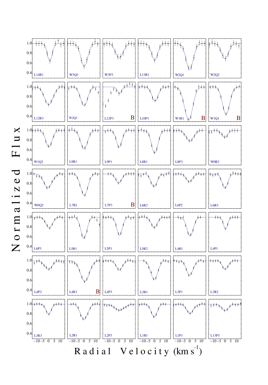
Figure 1: Profiles of selected H₂ lines in the absorption system toward Q 0347$-$383. The letter “B” marks lines which have a good profile but do not satisfy the selection criteria (see Section 4, and Fig. 3). The zero point of the radial velocity corresponds to the redshift $z_{\rm abs}=3.0249$.

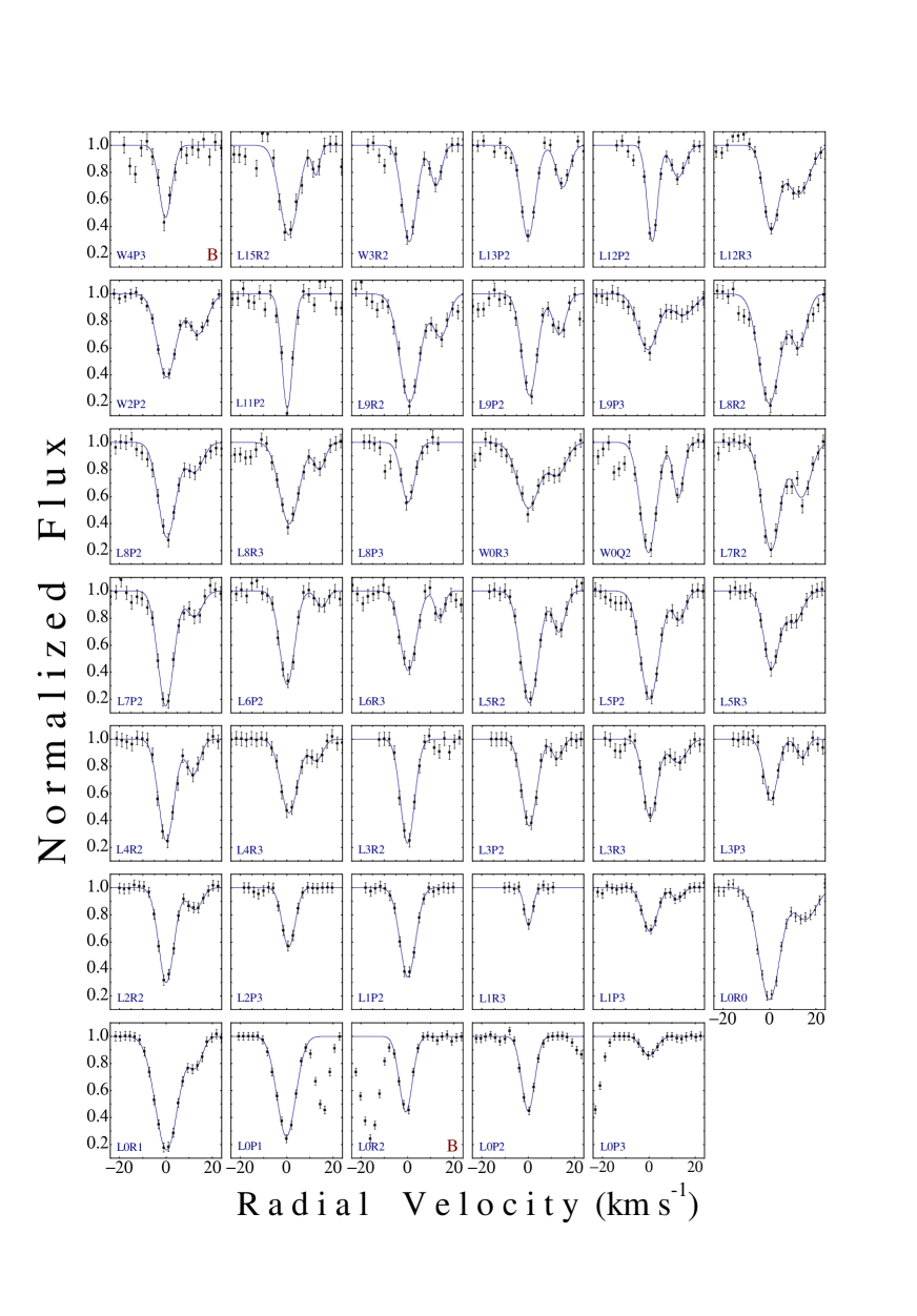
Figure 2: Profiles of selected H₂ lines in the absorption system toward Q 0405$-$443. The letter “B” marks lines which have a good profile but do not satisfy the selection criteria (see section 4, and Fig. 3). The zero point of the radial velocity corresponds to the redshift $z_{\rm abs}=2.5947$.

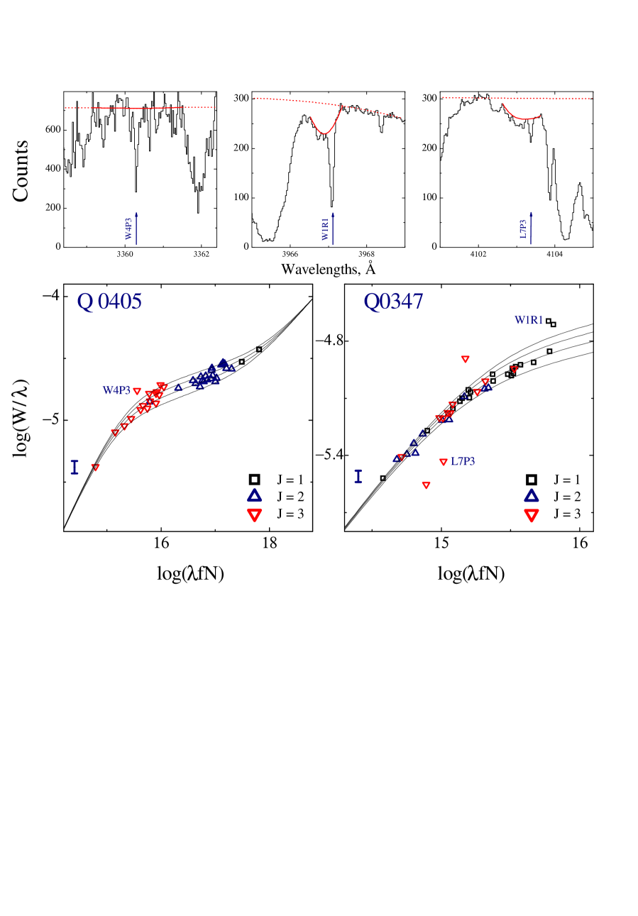
Figure 3: Curves of growth for the observed absorption lines (bottom panels; $\,\lambda$[Å], N[cm^-2]). The three top panels illustrate the procedure we use to fix the local continuum (solid bold line). The equivalent widths for the W4P3 and W1R1 lines (first and second top panels) lie above the corresponding curves of growth. It means that the lines are probably blended. The equivalent widths for L7P3 line (third top panel) lies under the curve of growth. It means that the real continuum (dash line) probably lies above the local one. In the analysis, we do not use these lines as well as other lines that are not on the curve of growth. (The error bars on the bottom panels show typical errors for the plotted points).

We used the UVES echelle spectrograph mounted on the Very Large Telescope of the European Southern Observatory to obtain new and better quality data (compared to what was available in the UVES data base) on two high-redshift ($z_{\rm em}$ = 3.22 and 3.02) bright quasars, respectively Q 0347$-$383 and Q 0405$-$443. Nine exposures of 1.5 h each were taken for each of the quasars over six nights under sub-arcsec seeing conditions in January 2002 and 2003 for, respectively, Q 0347$-$383 and Q 0405$-$443. The slit was 0.8 arcsec wide resulting in a resolution of R $\sim$ 53000 over the wavelength range 3290-4515 Å. Thorium-Argon calibration data were taken with different slit widths (from 0.8 to 1.4 arcsec) before and after each exposure and data reduction was performed using these different calibration settings to ensure accurate wavelength calibration. Spectra were extracted using procedures implemented in MIDAS, the ESO data reduction package. The reduction is particularly robust as only one CCD is used for the observations (setting #390). We have extracted the lamp spectra in the same way as the science spectra and checked that there is no systematic shift in the position of the emission lines.

Possible systematic effects leading to wavelength mis-calibration have been discussed by Murphy et al. (Murphy (2001)) and we specify here a few technical points. The wavelength calibration has been extensively checked using ThAr lamps. Errors measured from the lamp spectra are typically $\sim 2$ mÅ. Air-vacuum wavelength conversion has been made using the Edlén (edlen (1966)) formula at $15^{\rm o}\,$C. A shift in the wavelength scale can be introduced if the Thorium-Argon lamp and the science spectra are taken at systematically different temperatures and pressures. This is not the case here as calibration spectra were taken just before and after the science exposures. The temperature variations measured over one night in UVES are smaller than 0.5 K (see Dekker et al. dekker (2000)). Heliocentric correction is done using Stumpff (Stumpff (1980)) formula. In addition, all exposures were taken with the slit aligned with the parallactic angle so that atmospheric dispersion has little effect on our measurements. Therefore, as discussed by Murphy et al. (Murphy (2001)), uncertainties due to these effects are neligible.

4 Data Analysis

In each of the quasar spectra there is a damped Lyman-$\alpha$ system in which H₂ has been well studied, at $z_{\rm abs}$ = 3.0249 (Levshakov et al. 2002b , Ledoux et al. led03 (2003)), and 2.5947 (Ledoux et al. led03 (2003)) for Q 0347$-$383 and Q 0405$-$443, respectively. A crucial advantage of these H₂ absorption systems is that numerous unsaturated lines with narrow simple profiles are seen. A single component profile is sufficient to fit the lines on the line of sight toward Q 0347$-$383 and profiles of two well separated ($\Delta V$ = 13 km s^-1) components are fitted in the case of Q 0405$-$443. The absorption lines are shown in Fig. 1 and  2 for the two quasars respectively. For the latter object, we fitted the two components but discuss only the positions of the strongest one in the following.

4.1 Selection of lines

We selected H₂ lines that are not obviously blended with other narrow absorptions, in particular H i intervening Lyman-$\alpha$ lines, and that have normalized central intensities larger than 0.1 and smaller than 0.9. The 82 selected lines (42 toward Q 0347$-$383 and 40 toward Q 0405$-$443) were fitted with Voigt profiles estimating the continuum locally. Possible hidden inaccuracy or problems related to individual lines (inacurate continuum determination, possible non-obvious blends, etc…) were checked by constructing curves of growth for the two sets of molecular lines (Fig. 3). For this, we plot log($W/\lambda$) versus log($\lambda fN$) for the lines observed along both lines of sight (see Fig. 3) together with theoretical curves corresponding to Doppler parameters $b$ = 1.7, 1.5, 1.3, and 1.1 km s^-1. It is apparent from the figure that 5 lines toward Q 0347$-$383 and one line toward Q 0405$-$443 do not lie on the theoretical curves. This is probably a consequence of blending with other lines in the Lyman-$\alpha$ forest and/or difficulties in positioning the continuum as illustrated for three of these lines in the top panels of Fig. 3. The six lines are marked with a sign ”B” in Figs. 1 and 2 and are not considered in the following analysis which is therefore based on 76 lines (37 toward Q 0347$-$383 and 39 toward Q 0405$-$443).

For the selected lines, the curves of growth analysis gives the column density (for each rotational level), $N_{\rm J}$ [cm^-2], and the Doppler parameter $b$. For the Q 0405$-$443 absorption system, $\log N_{\rm J=1}=17.7\pm 0.2$, $\log N_{\rm J=2}=15.9\pm 0.3$, $\log N_{\rm J=3}=14.7\pm 0.3$, and $b$ = 1.4$\pm$0.3 km s^-1. For the Q 0347$-$383 absorption system $\log N_{\rm J=1}=14.3\pm 0.2$, $\log N_{\rm J=2}=13.8\pm 0.2$, $\log N_{\rm J=3}=14.0\pm 0.2$, and b = 1.3$\pm$0.2 km s^-1.

4.2 Line parameters

The atomic parameters of the selected lines are given in Tables 1 and 2. The first column specifies the lines. The second one gives the sensitivity coefficients $K_{\rm i}$. The 3rd and 4th columns present the observed wavelengths and their errors, $\lambda_{\rm i}$ and $\sigma_{\lambda_{i}}$. The 5th and 6th columns give the rest wavelengths, $\lambda_{\rm i}^{\rm lab}$, as estimated in different laboratory experiments. The first estimate (called $\lambda^{\rm a}_{\rm i}$) is obtained using level energies (Jennings et al. Jen84 (1984), Dabrowski dab84 (1984), Abgrall et al. Abgr (1993), Roncin & Launay Ron (1994)) determined from laboratory observations of the H₂ emission spectrum. Uncertainties for the ground state energies are less than $3\times 10^{-4}$ cm^-1 (Jennings et al. Jen84 (1984)). Uncertainties are more difficult to estimate for the upper levels although close to 0.1 cm^-1 (Dabrowski dab84 (1984)) for most of the lines. This means that most of the errors are of the same order of magnitude as our observational measurements, 1 mÅ  in the rest frame (or about 3 to 4 mÅ  for the observer). The second estimate (called $\lambda^{\rm p}_{\rm i}$) is a direct measurement using a narrow-band tunable extreme UV laser source (Philip et al. 2004). This experiment is supposed to be much more precise and errors should be less than 0.011 cm^-1.

Observational errors ($\sigma_{\lambda_{i}}$) are of the order of 3 mÅ, they characterize only the accuracy of the profile fitting of the observed lines by gaussian profiles. The total error of the line centrum position can be estimate from the real dispersion of points (e.g. Fig.5.) $\sigma_{\lambda_{i}}\;\raise 1.29167pt\hbox{$<$\kern-7.5pt\raise-4.73611pt\hbox{$\sim$}}\;\lambda^{lab}\sigma_{z_{i}}\approx 5$mÅ.

4.3 Consistency of the two lines of sight

An important internal check of the data quality consists in comparing measurements of the eight lines present in both QSO spectra. This is done in Fig. 4 where the relative positions, $\zeta_{\rm i}=(z_{\rm i}^{\rm obs}-\bar{z})/(1+\bar{z})\;$, is plotted versus $K_{\rm i}$; $\bar{z}$ being the median redshift (i.e. model independent) of all H₂ lines observed in one spectrum. It can be seen that all measurements are within observational errors (at the 2$\sigma$ level). As the two lines of sight have been observed and reduced independently, this shows that the data calibration and the measurement procedure are reliable at the level required for the study.

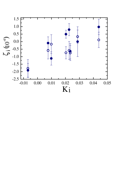
Figure 4: The relative positions, $\zeta_{\rm i}=(z_{\rm i}-\bar{z})/(1+\bar{z})$, of lines observed in the spectra of both quasars Q 0405$-$443 (filled circles) and Q 0347$-$383 (open circles) are plotted versus the sensitivity coefficient $K_{\rm i}$. Here, $\bar{z}$ is the median redshift of all H₂ lines observed in the one corresponding spectrum. The lines are L3R3, L3R2, L5R2, L6R3, L6P2, W0Q2, L8P3, and L12R3 and $\lambda_{\rm lab}^{\rm a}$ are used. The 1 $\sigma$ error bars shown are observational (without laboratory errors). They are of the order of 3 mÅ  (in the observer’s frame). It can be seen that both sets of measurements are mutually consistent within observational errors. The fact that the two independent observational measurements agree well indicates that our data calibration and measurement procedure are reliable at the level required for the study.

Table 1:  Parameters of H₂ lines for the absorption system at z=3.02490 in the spectrum of Q 0347-383.

Lines $$K_{i}$$ , Å , Å , Å , Å

L14R1 0.05495 3811.506 0.0025 946.9795 946.98040

W 3Q1 0.02176 3813.279 0.0022 947.4212 947.42188

W 3P3 0.01724 3830.382 0.0023 951.6711 951.67186

L13R1 0.05109 3844.044 0.0024 955.0649 955.06582

L13P3 0.04574 3865.717 0.0027 960.4497 960.45063

W 2Q1 0.01423 3888.435 0.0013 966.0951 966.09608

W 2Q2 0.01301 3893.205 0.0020 967.2800 967.28110

L12R3 0.04386 3894.800 0.0020 967.6758 967.67695

W 2Q3 0.01120 3900.325 0.0015 969.0481 969.04922

L10P1 0.04053 3955.815 0.0017 982.8339 982.83533

W 1Q2 0.00394 3976.499 0.0035 987.9743 987.97445

L 9R1 0.03796 3992.767 0.0017 992.0156 992.01637

L 9P1 0.03719 3995.960 0.0010 992.8093 992.80968

L 8R1 0.03444 4034.769 0.0008 1002.4509 1002.45210

L 8P3 0.02872 4058.651 0.0018 1008.3849 1008.38615

W 0R2 -0.00503 4061.220 0.0030 1009.0244 1009.02492

W 0Q2 -0.00686 4068.922 0.0024 1010.9389 1010.93844

L 7R1 0.03062 4078.983 0.0017 1013.4364 1013.43701

L 6R2 0.02496 4131.669 0.0028 1026.5281 –

L 6P2 0.02347 4138.020 0.0021 1028.1055 1028.10609

L 6R3 0.02262 4141.563 0.0025 1028.9856 –

L 6P3 0.02053 4150.451 0.0014 1031.1917 1031.19260

L 5R1 0.02183 4174.421 0.0020 1037.1490 1037.14992

L 5P1 0.02088 4178.483 0.0015 1038.1568 1038.15713

L 5R2 0.02038 4180.622 0.0017 1038.6901 1038.69027

L 4R1 0.01681 4225.987 0.0026 1049.9592 1049.95976

L 4P1 0.01580 4230.303 0.0025 1051.0317 1051.03253

L 4P2 0.01369 4239.360 0.0040 1053.2841 1053.28426

L 4P3 0.01071 4252.193 0.0010 1056.4709 1056.47143

L 3R1 0.01132 4280.316 0.0020 1063.4594 1063.46014

L 3P1 0.01026 4284.928 0.0015 1064.6048 1064.60539

L 3R2 0.00989 4286.499 0.0027 1064.9950 1064.99481

L 3R3 0.00758 4296.491 0.0024 1067.4780 1067.47855

L 2R1 0.00535 4337.628 0.0025 1077.6979 1077.69894

L 2P3 -0.00098 4365.242 0.0027 1084.5593 1084.56034

L 1R1 -0.00113 4398.132 0.0015 1092.7316 –

L 1P1 -0.00234 4403.449 0.0030 1094.0516 –

^a H₂ laboratory wavelengths are from (Jennings et al. Jen84 (1984), Dabrowski dab84 (1984), Abgrall et al. Abgr (1993), Roncin & Launay Ron (1994)).
^p H₂ laboratory wavelengths are from (Philip et al. 2004).

Table 2:  Parameters of H₂ lines for the absorption system at z=2.59473 in the spectrum of Q 0405-443.

Lines $$K_{i}$$ , Å , Å , Å , Å

L15R2 0.05816 3381.302 0.0030 940.6257 –

W 3R2 0.02193 3404.619 0.0019 947.1116 947.11169

L13P2 0.04848 3442.500 0.0025 957.6516 957.65223

L12P2 0.04503 3473.513 0.0023 966.2751 966.27550

L12R3 0.04386 3478.541 0.0018 967.6758 967.67695

W 2P2 0.01198 3480.759 0.0015 968.2943 968.29522

L11P2 0.04177 3506.107 0.0023 975.3454 975.34576

L 9R2 0.03647 3571.558 0.0018 993.5505 993.55061

L 9P2 0.03519 3576.309 0.0022 994.8735 994.87408

L 9P3 0.03232 3586.919 0.0035 997.8264 997.82717

L 8R2 0.03296 3609.057 0.0034 1003.9851 1003.98545

L 8P2 0.03161 3614.121 0.0025 1005.3923 1005.39320

L 8R3 0.03061 3617.795 0.0018 1006.4130 1006.41416

L 8P3 0.02872 3624.876 0.0036 1008.3849 1008.38615

W 0R3 -0.00617 3631.147 0.0025 1010.1304 1010.13025

W 0Q2 -0.00682 3634.050 0.0017 1010.9389 1010.93844

L 7R2 0.02914 3648.575 0.0025 1014.9767 1014.97685

L 7P2 0.02772 3653.904 0.0024 1016.4612 1016.46125

L 6P2 0.02347 3695.764 0.0019 1028.1056 1028.10609

L 6R3 0.02262 3698.933 0.0015 1028.9856 –

L 5R2 0.02038 3733.817 0.0010 1038.6901 1038.69027

L 5P2 0.01880 3739.844 0.0010 1040.3672 1040.36732

L 5R3 0.01805 3742.691 0.0017 1041.1583 1041.15892

L 4R2 0.01536 3779.856 0.0021 1051.4988 1051.49857

L 4R3 0.01304 3788.770 0.0015 1053.9753 1053.97610

L 3R2 0.00989 3828.370 0.0017 1064.9950 1064.99481

L 3P2 0.00812 3835.227 0.0020 1066.9006 1066.90068

L 3R3 0.00758 3837.300 0.0016 1067.4781 1067.47855

L 3P3 0.00511 3846.871 0.0023 1070.1401 1070.14087

L 2R2 0.00394 3879.528 0.0021 1079.2259 1079.22491

L 2P3 -0.00098 3898.707 0.0024 1084.5593 1084.56034

L 1P2 -0.00453 3941.405 0.0020 1096.4390 –

L 1R3 -0.00479 3942.435 0.0029 1096.7246 –

L 1P3 -0.00760 3953.441 0.0014 1099.7864 –

L 0R0 -0.00772 3983.420 0.0020 1108.1277 –

L 0R1 -0.00818 3985.240 0.0018 1108.6328 –

L 0P1 -0.00948 3990.370 0.0020 1110.0617 –

L 0P2 -0.01170 3999.123 0.0013 1112.4963 –

L 0R3 -0.01178 3999.437 0.0020 1112.5830 –

^a H₂ laboratory wavelengths are from (Jennings et al. Jen84 (1984), Dabrowski dab84 (1984), Abgrall et al. Abgr (1993), Roncin & Launay Ron (1994)).
^p H₂ laboratory wavelengths are from (Philip et al. 2004).

5 Results

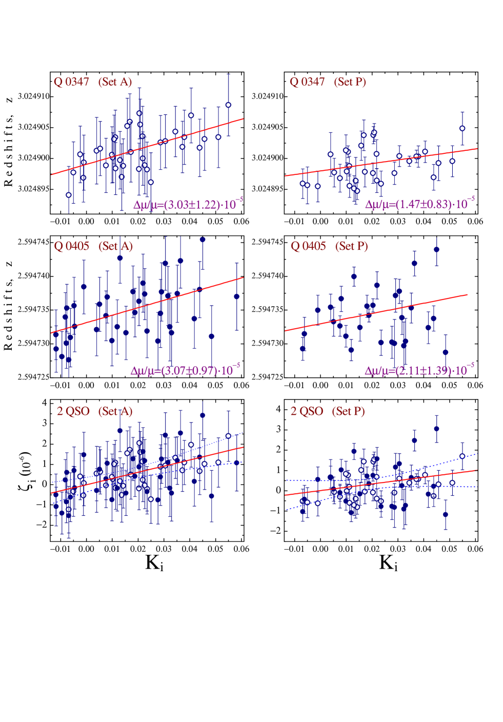
Figure 5: Regression analysis using rest wavelengths from energy levels (Sample A; left column) and from laser experiments (Sample P; right column) for both quasars (top and middle rows) and the whole sample (bottom row).

In Fig. 5 we plot $z_{\rm i}$ versus $K_{\rm i}$ for absorption lines observed in the spectra of Q 0347$-$383 (open circles) and Q 0405$-$443 (filled circles) respectively. The left hand side panels corresponds to rest-wavelengths $\lambda_{\rm lab}^{\rm a}$ and the right hand side panel to rest-wavelengths $\lambda_{\rm lab}^{\rm p}$. The best fit of the linear regression $z_{\rm i}$-to-$K_{\rm i}$ in accordance with Eq. (2) is overplotted in all panels.

For the left hand side panels, error bars are the combination of measurement errors (evaluated from col. 5 of Tables 1 and 2) with an error of 1 mÅ, in the rest frame, to account for uncertainties in laboratory wavelength determination. For the right hand side panels, uncertainties in laboratory wavelength determination are supposed to be of the order of 0.1 mÅ.

Data for both quasars are combined in the bottom panels using the following formula for reduced redshift $\zeta_{\rm i}$:

$$\zeta_{\rm i}=\frac{z_{\rm i}^{\rm obs}-z_{\rm abs}}{1+z_{\rm abs}}$$ (3)

In this formula, $z_{\rm abs}$ is obtained from the best linear fit of the data in accordance with Eq. (2). They are $z_{\rm abs}=3.02489904(120)$ for Q 0347$-$383 and $z_{\rm abs}=2.59473315(81)$ for Q 0405$-$443.

The results of the linear regression analysis are presented in Table 3. The first column gives the QSO name, the second one gives the number of lines used in the regression analysis, the third column gives the estimated value of $\Delta\mu/\mu$. Estimates of $\Delta\mu/\mu$ are given using the two sets of rest wavelengths for both quasars separately as well as for the combined sample. Most of the lines are from J = 1 for Q 0347$-$383 and J = 2 for Q 0405$-$443 and the results of the regression analysis for these two subsamples are also given. Note that the number of lines is smaller in the case where $\lambda_{\rm lab}^{\rm p}$ are used because not all the lines have been measured.

Table 3: $\Delta\mu/\mu$ estimates from different samples.

$$\begin{array}[]{lcc}\hline\cr\hline\cr\vskip 3.0pt plus 1.0pt minus 1.0pt\cr&\leavevmode\nobreak\ \mbox{N.\leavevmode\nobreak\ of\leavevmode\nobreak\ L.}\nobreak\leavevmode&\leavevmode\nobreak\ \Delta\mu/\mu\nobreak\leavevmode\\ \vskip 3.0pt plus 1.0pt minus 1.0pt\cr\hline\cr\vskip 3.0pt plus 1.0pt minus 1.0pt\cr&\mbox{Set (A)}&\\ \hline\cr\vskip 3.0pt plus 1.0pt minus 1.0pt\cr\leavevmode\nobreak\ \mbox{Q\leavevmode\nobreak\ 0347$-$383}\nobreak\leavevmode&\leavevmode\nobreak\ \leavevmode\nobreak\ 37\nobreak\leavevmode\nobreak\leavevmode&\leavevmode\nobreak\ (3.03\pm 1.22)\times 10^{-5}\nobreak\leavevmode\\ \vskip 3.0pt plus 1.0pt minus 1.0pt\cr\vskip 3.0pt plus 1.0pt minus 1.0pt\cr\leavevmode\nobreak\ \mbox{Q\leavevmode\nobreak\ 0347$-$383\leavevmode\nobreak\ \leavevmode\nobreak\ (J=1)}\nobreak\leavevmode&\leavevmode\nobreak\ \leavevmode\nobreak\ 18\nobreak\leavevmode\nobreak\leavevmode&\leavevmode\nobreak\ (3.23\pm 1.63)\times 10^{-5}\nobreak\leavevmode\\ \vskip 3.0pt plus 1.0pt minus 1.0pt\cr\vskip 3.0pt plus 1.0pt minus 1.0pt\cr\leavevmode\nobreak\ \mbox{Q\leavevmode\nobreak\ 0405$-$443}\nobreak\leavevmode&\leavevmode\nobreak\ \leavevmode\nobreak\ 39\nobreak\leavevmode\nobreak\leavevmode&\leavevmode\nobreak\ (3.07\pm 0.97)\times 10^{-5}\nobreak\leavevmode\\ \vskip 3.0pt plus 1.0pt minus 1.0pt\cr\vskip 3.0pt plus 1.0pt minus 1.0pt\cr\leavevmode\nobreak\ \mbox{Q\leavevmode\nobreak\ 0405$-$443\leavevmode\nobreak\ \leavevmode\nobreak\ (J=2)}\nobreak\leavevmode&\leavevmode\nobreak\ \leavevmode\nobreak\ 22\nobreak\leavevmode\nobreak\leavevmode&\leavevmode\nobreak\ (3.78\pm 1.36)\times 10^{-5}\nobreak\leavevmode\\ \vskip 3.0pt plus 1.0pt minus 1.0pt\cr\vskip 3.0pt plus 1.0pt minus 1.0pt\cr\leavevmode\nobreak\ \mbox{2\leavevmode\nobreak\ QSO}\nobreak\leavevmode&\leavevmode\nobreak\ \leavevmode\nobreak\ 76\nobreak\leavevmode\nobreak\leavevmode&\leavevmode\nobreak\ (3.05\pm 0.75)\times 10^{-5}\nobreak\leavevmode\\ \vskip 3.0pt plus 1.0pt minus 1.0pt\cr\hline\cr\vskip 3.0pt plus 1.0pt minus 1.0pt\cr&\mbox{Set (P)}&\\ \hline\cr\vskip 3.0pt plus 1.0pt minus 1.0pt\cr\leavevmode\nobreak\ \mbox{Q\leavevmode\nobreak\ 0347$-$383}\nobreak\leavevmode&\leavevmode\nobreak\ \leavevmode\nobreak\ 33\nobreak\leavevmode\nobreak\leavevmode&\leavevmode\nobreak\ (1.47\pm 0.83)\times 10^{-5}\nobreak\leavevmode\\ \vskip 3.0pt plus 1.0pt minus 1.0pt\cr\vskip 3.0pt plus 1.0pt minus 1.0pt\cr\leavevmode\nobreak\ \mbox{Q\leavevmode\nobreak\ 0405$-$443}\nobreak\leavevmode&\leavevmode\nobreak\ \leavevmode\nobreak\ 29\nobreak\leavevmode\nobreak\leavevmode&\leavevmode\nobreak\ (2.11\pm 1.39)\times 10^{-5}\nobreak\leavevmode\\ \vskip 3.0pt plus 1.0pt minus 1.0pt\cr\vskip 3.0pt plus 1.0pt minus 1.0pt\cr\leavevmode\nobreak\ \mbox{2\leavevmode\nobreak\ QSO}\nobreak\leavevmode&\leavevmode\nobreak\ \leavevmode\nobreak\ 62\nobreak\leavevmode\nobreak\leavevmode&\leavevmode\nobreak\ (1.65\pm 0.74)\times 10^{-5}\nobreak\leavevmode\\ \vskip 3.0pt plus 1.0pt minus 1.0pt\cr\hline\cr\hline\cr\end{array}$$

Systematic effects in measurements of the central position of a line profile were discussed by Ivanchik et al. (IAV2 (1999)) and in more detail by Murphy et al. (Murphy (2001)). Here we discuss two possible sources of systematic errors more specifically.

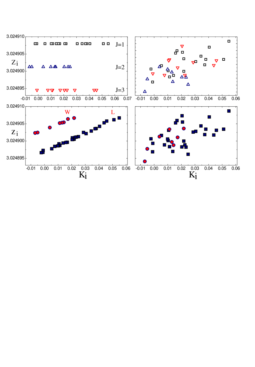
Figure 6: Possible systematic effects. The left top panel illustrates the kinematic effect that could arise if absorption lines from different rotational levels J had different velocity positions in the spectrum (Jenkins & Peimbert, JP (1997)). It may mimic $\mu$-variation if ranges of $K_{\rm i}$ for different J levels do not overlap. The observed situation is shown in the right top panel. The $K_{\rm i}$ ranges for J = 1 and J = 3 overlap enough and slopes are similar for each J levels within the statistical uncertainties. The second type of systematic error could be a consequence of any effect that could produce a shift increasing monotonously with wavelength: H₂ laboratory wavelengths, and/or Th-Ar calibration, air-vacuum wavelength conversion, atmospheric dispersion effects, instrumental profile variation with $\lambda$ etc… (Murphy et al., Murphy (2001))). In that case, the regression lines for Lyman and Werner bands should be shifted from one to the other (bottom left panel). It is apparent from the observation (bottom right panel) that such an effect cannot be the dominant source of the correlation.

The first one may be called the kinematic effect. Due to peculiar structure in the clouds H₂ molecular features from different rotational levels J = 0, 1, 2, 3… may not be produced in the same region of the absorbing cloud and therefore may have different mean observed velocities (e.g. Jenkins & Peimbert, JP (1997)). This could lead to relative shifts between the common redshifts derived for lines from different rotational levels J. This is illustrated in Fig. 6. The top left panel shows the ideal $z$-$K_{\rm i}$ relation (for $\Delta\mu$ = 0) for a sample of J = 1, 2, 3 lines corresponding to the lines observed toward Q 0347$-$383 for which we have imposed a shift of 0.5 km s^-1 between different J levels. This effect could mimic $\mu$-variation if ranges of $K_{\rm i}$ for different J levels do not overlap. The observed situation is shown in the top-right panel of the same figure. In that case, the overlap between $K_{\rm i}$ ranges for J = 1 and J = 3 lines is important enough so that the correlation cannot be due to this effect. Moreover, most of the lines (18 out of 37) are from the J = 1 level and the linear regression analysis for these lines only gives a $\Delta\mu/\mu$ value similar to what is derived from the whole sample (see Tables 3).

Another systematic error could be produced by any effect producing a shift monotonically increasing with increasing wavelength. This could be a consequence of slightly unprecise Th-Ar calibration or air-vacuum wavelength conversion, or atmospheric dispersion effects, instrumental profile variation etc… (Murphy et al., Murphy (2001)). Indeed, there is a well-known correlation between $K_{\rm i}$ and $\lambda_{0}$. Such effects could lead to a slope in the regression line, i.e. mimic $\mu$-variation. This is illustrated in the bottom-left panel of Fig. 6 where such an ideal artificial effect has been applied to the sample of lines seen toward Q 0347$-$383. It can be seen however that the Werner and Lyman-band lines have different locations in the plane. The reason is that for the same $K_{\rm i}$ coefficient, the Werner lines have larger $\lambda_{0}$. It is apparent from the observed sample (bottom-right panel) that there is no such shift.

6 Conclusion

Using 76 H₂ absorption lines observed at $z_{\rm abs}$ = 2.59473 and 3.02490 in the spectra of two quasars, respectively, Q 0405$-$443 and Q 0347$-$383, we have searched for any correlation between the relative positions of H₂ absorption lines measured as $\zeta_{\rm i}$ = ($z_{\rm i}-{\bar{z}}$)/(1+${\bar{z}}$) and the sensitivity coefficients $K_{\rm i}$ of the lines to a change in $\mu$. A positive correlation could be interpreted as a variation of the proton-to-electron mass ratio, $\Delta\mu$/$\mu$. We use two sets of rest wavelengths as estimated from different laboratory experiments. Wavelengths derived from energy level determination give $\Delta\mu$/$\mu$ = (3.05$\pm$0.75)$\times$10^-5, over the past $\sim$12 Gyrs. However, wavelengths derived from a direct and, in principle, more precise determination using laser techniques give $\Delta\mu$/$\mu$ = (1.64$\pm$0.74)$\times$10^-5. The latter limit is the most stringent limit obtained to date now on the variation of this fundamental constant. This limit, together with the limit on $\Delta\alpha/\alpha$, yields an estimate of the $R$ parameter defined as $\Delta\mu/\mu\simeq R\Delta\alpha/\alpha$. Using $\Delta\alpha/\alpha$ from Murphy et al. (Murphy03 (2003)) gives $\,-9.5\leq R\leq-0.2\,$, and $\Delta\alpha/\alpha$ from Chand et al. (Chand (2004)) gives $|R|>1$ (at the $2\sigma$ C.L.).

- (1) Abgrall, H., Roueff, E., Launay, F., Roncin, J.-Y., & Subtil, J.-L. 1993, J. of Mol. Spec., 157, 512
- (2) Calmet, X., & Fritzsch, H. 2002, Eur. Phys. J., C24, 639
- (3) Chand, H., Srianand, R., Petitjean, P., & Aracil, B. 2004, A&A, 417, 853
- (4) Cowie, L., & Songaila, A. 1995, ApJ, 453, 596
- (5) Dabrowski, I. 1984, Can. J. Phys., 62, 1639
- (6) Dekker, H., D’Odorico, S., Kaufer, A., Delabre, B., & Kotzlowski, H. 2000, SPIE 4008, 534
- (7) Dent, T., & Fairbairn, M. 2003, Nuc. Phys. B, 653, 256
- (8) Dine, M., Nir, Y., Raz, G., & Volansky, T. 2003, Phys. Rev. D, 67, 015009
- (9) Dzuba, V., Flambaum, V., & Webb, J. 1999, Phys. Rev. A., 59, 230
- (10) Edlén, B. 1966, Metrologia, 2, 71
- (11) Ivanchik, A., Potekhin, A., & Varshalovich, D. 1999, A&A, 343, 439
- (12) Ivanchik, A., Petitjean, P., Rodriguez, E., & Varshalovich, D. 2003, Astrophys. Space Sci., 283, 583
- (13) Jenkins, E.B., & Peimbert, A. 1997, ApJ, 477, 265
- (14) Jennings, D.E., Bragg, S.L., & Brault, J.W. 1984, ApJ, 282, L85
- (15) Langacker, P., Segre, G., & Strassler, M. 2002, Phys. Lett., B528, 121
- (16) Ledoux, C., Petitjean, P., & Srianand, R., 2003, MNRAS, 346, 209
- (17) Levshakov, S., Dessauges-Zavadsky, M., D’Odorico, S., & Molaro, P. 2002a, MNRAS, 333, 373
- (18) Levshakov, S., Dessauges-Zavadsky, M., D’Odorico, S., & Molaro, P. 2002b, ApJ, 565, 696
- (19) Mohr, P.J., & Taylor, B.N. 2002, CODATA Recommended Values of the Fundamental Physical Constants: 2002, (http://physics.nist.gov/), to be published.
- (20) Murphy, M., Webb, J., Flambaum, V., Churchill, C., & Prochaska, J. 2001, MNRAS, 327, 1223
- (21) Murphy, M., Webb, J., & Flambaum, V. 2003, MNRAS, 345, 609
- (22) Olive, K.A., Pospelov, M., Qian, Y.-Z., Coc, A., Casse, M., & Vangioni-Flam, E. 2002, Phys. Rev., D66, 045022
- (23) Philip, J., Sprengers, J.P., Pielage, Th., Lange, C.A., Ubachs, W., & Reinhold, E. 2004, Can. J. Chem., 82, 713
- (24) Potekhin, A., Ivanchik, A., Varshalovich, D., Lanzetta, K., Baldwin, J., Williger, G., & Carswell, R. 1998, ApJ, 505, 523
- (25) Quast, R., Reimers, D., & Levshakov, S. 2004, A&A, 415, L7
- (26) Roncin, J.-Y. & Launay, F. 1994, Journal Phys. and Chem. Reference Data, No. 4
- (27) Srianand, R., Chand, H., Petitjean, P., & Aracil, B. 2004, PRL, 92, 121302
- (28) Stumpff, P. 1980, A&AS, 41, 1
- (29) Ubachs, W., & Reinhold, E. 2004, PRL, 92, 101302
- (30) Varshalovich, D., & Levshakov, S. 1993, JETP Letters, 58, 231
- (31) Varshalovich, D., & Potekhin, A. 1995, Space Sci. Rev., 74, 259
- (32) Webb, J., Flambaum, V., Churchill, C., Drinkwater, M., & Barrow, J. 1999, Phys. Rev. Lett., 82, 884