CH₃OH abundance in low mass protostars

We present observations of methanol lines in a sample of Class 0 low mass protostars. Using a 1-D radiative transfer model, we derive the abundances in the envelopes. In two sources of the sample, the observations can only be reproduced by the model if the methanol abundance is enhanced by about two order of magnitude in the inner hot region of the envelope. Two other sources show similar jumps, although at a lower confidence level. The observations for the other three sources are well reproduced with a constant abundance, but the presence of a jump cannot be ruled out. The observed methanol abundances in the warm gas around low mass protostars are orders of magnitude higher than gas phase chemistry models predict. Hence, in agreement with other evidence, this suggests that the high methanol abundance reflects recent evaporation of ices due to the heating by the newly formed star. The observed abundance ratios of CH₃OH, H₂CO and CO are in good agreement with grain surface chemistry models. However, the absolute abundances are more difficult to reproduce and may indicate the presence of multiple ice components in these regions.

1 Introduction

During the formation of a star, the gas undergoes important physical and chemical changes. In the prestellar phase, the gas is heavily depleted by accretion on grain mantles. When the gravitational collapse starts, the protostar warms the gas while ice mantle molecules are released into the gas phase. These released molecules trigger the formation of more complex molecules through rapid reactions in the warm gas (Charnley et al. 1992).

While the importance of ice mantle evaporation and hot core chemistry around high mass protostars was known well over a decade ago, the existence of such regions in low mass protostars has been established more recently. Ceccarelli et al. (2000a, b) have shown that H₂O and H₂CO abundances in the low mass protostar IRAS16293-2422 are increased in the warm and dense inner part of the circumstellar envelope. In this region, H₂O and H₂CO are evaporated from the grain mantles and are injected in the gaseous phase. These findings were later confirmed by Schöier et al. (2002), who found strong evidence for the increase of several other molecular abundances (e.g. CH₃OH, SO and SO₂). Evaporation of H₂O has also been shown around one other Class 0 protostar, NGC1333-IRAS4 (Maret et al. 2002). Recently, Maret et al. (2004, Paper I) carried out a survey of the emission of H₂CO in a sample of nine low mass protostars, and concluded that in all the observed protostars but one, H₂CO is between two and three orders of magnitude more abundant in the inner part of the envelope than in the outer part, suggesting that the evaporation of grain mantles is a common phenomenon in the inner parts of low mass protostars.

While the importance of grain mantle evaporation is now well established in low mass protostars, the question of whether these molecules will form “daughter” molecules by hot core chemistry (Charnley et al. 1992) is still open. From a theoretical point of view, if the protostar is undergoing collapse, only very rapidly formed second-generation complex molecules can be produced. As noted by Schöier et al. (2002) if the protostar is in free fall, the evaporated molecules will fall on the central object in a few hundreds years. Hence, while evaporation can still occur on such a rapid timescale, the composition of the gas phase is then ‘frozen’ in, because the dynamical time scale is much shorter than the time needed to form second generation molecules (Rodgers & Charnley 2003). However, observationally, the recent detections of complex O and N bearing molecules – typical of massive hot cores – towards IRAS162293-2422 (Cazaux et al. 2003; Bottinelli et al. 2004b) and NGC1333-IRAS4A (Bottinelli et al. 2004a) are challenging these theoretical concepts, emphasising that the chemistry in low mass protostar envelopes is still poorly understood and needs to be further investigated.

Methanol is particularly suited for the study of hot cores around low mass protostars, because it is relatively abundant in grain mantles and dominates the organic content of evaporation zones. Indeed, such enrichments of methanol have already been observed in the inner regions of high mass protostars (van der Tak et al. 2000a), and in the gas shocked by prostellar outflows (Bachiller et al. 1998; Buckle & Fuller 2002). Moreover, methanol, being a slightly asymmetric-top molecule, can be used to probe a large range of physical conditions, both in density and temperature (e.g. Leurini et al. 2004). The recent computations of collisional rate coefficients of methanol with para-H₂ (Pottage et al. 2004) make precise determination of these conditions possible.

In this paper, observations of methanol transitions from low mass protostars are presented. A detailed radiative transfer model is used to derive the methanol abundance inside the protostellar envelopes. Finally, the methanol abundances in the envelopes are compared to those in other environments, and the implications for the formation of this molecule are discussed.

2 Observations

Six Class 0 protostars (see Table 1) were observed using the Institut de Radio-Astronomie Millimétrique 30 meters telescope (IRAM-30m), and the James Clerk Maxwell Telescope (JCMT). The methanol 5_K-4_K transitions were observed with the IRAM-30m telescope, while the 7_K-6_K were observed with the JCMT. JCMT and CSO observations of IRAS16293-2422 from the literature were also used (van Dishoeck et al. 1995).

Table 1: The observed sample.

Source	$\alpha(2000)$	$\delta(2000)$	Cloud	Dist.a	$L_{\mathrm{bol}}$b	$M_{\mathrm{env}}$b	$L_{\mathrm{smm}}/L_{\mathrm{bol}}$c	$T_{\mathrm{bol}}$c
				(pc)	($L_{\sun}$)	($M_{\sun}$)	(%)	(K)
NGC1333-IRAS4A	03:29:10.3	+31:13:31	Perseus	220	6	2.3	5	34
NGC1333-IRAS4B	03:29:12.0	+31:13:09	Perseus	220	6	2.0	3	36
NGC1333-IRAS2	03:28:55.4	+31:14:35	Perseus	220	16	1.7	$\lesssim$ 1	50
L1448-MM	03:25:38.8	+30:44:05	Perseus	220	5	0.9	2	60
L1448-N	03:25:36.3	+30:45:15	Perseus	220	6	3.5	3	55
L1157-MM	20:39:06.2	+68:02:22	Isolated	325	11	1.6	5	60
IRAS16293-2422	16:32:22.7	-24:38:32	$\rho$-Ophiuchus	160	27	5.4	2	43

^a From André et al. (2000), except for Perseus sources (Černis 1990).
^b From Jørgensen et al. (2002).
^c From André et al. (2000).

The IRAM-30m observations were obtained in November 2002. The A230 and B230 receivers were used simultaneously with the autocorrelator, providing a spectral resolution of 0.5 km/s and a bandwidth of 320 MHz. The calibration and the pointing were regularly checked and were found to be better than 20% and 3″ respectively. For all the sources the observations were done in position switching mode, after checking that the reference position was free of line emission. In order to determine the spatial extent of the methanol emission, small maps of 3 by 3 pixels were made, with a 10″ sampling.

The JCMT observations were obtained in September 2000 and from February 2001 to February 2003. The B3 receiver was used with the digital autocorrelator spectrometer (DAS) in setup with a bandwith of 500 MHz and a spectral resolution of 0.4 km/s. As for the IRAM-30m observations, the pointing and calibration were regularly checked and was found to be better than 30% and 3″ respectively. A few lines already observed by van Dishoeck et al. (1995) towards IRAS16293-2422 were re-observed in September 2000. The lines fluxes from the two datasets were compared and were found to be in agreement within 30%. The JCMT observations were done in beam switching mode with a 180″ offset, large enough to avoid line contamination by the outflows or by the cloud.

3 Results

Fig. 1 and 2 show the spectra towards the six observed sources. Several 5-4 and 7-6 lines are detected in the bands observed with IRAM and JCMT respectively. The lines with lowest level energy (E_up $\sim$ 40 - 70 K) in each band are the brightest in the spectra and are detected toward all sources. On the contrary, only a few lines with larger upper level energies are detected in most sources, with NGC1333-IRAS2 showing the largest number of detected methanol lines (26 lines, up to upper level energies of 259 K). The relative intensity of the lines with low level energy to lines with high level energy varies from source to source, suggesting different excitation temperatures. The richer methanol spectrum of NGC1333-IRAS2 is, in this respect, likely due to a relatively larger excitation temperature with respect to other sources.

The lines with lowest level energy show, in some sources, bright high velocity wings, sometimes asymmetric. This is the case for NGC1333-IRAS4A, NGC1333-IRAS4B and NGC1333-IRAS2. In the other three sources (L1448-MM, L1448-N and L1557-MM), all the lines, including those with a low level energy, have relatively narrow Gaussian profiles (between 1 and 4 $\mathrm{km}\,\mathrm{s}^{-1}$) with much weaker broad wings, if any. Usually, large asymmetric wings testify to the presence of outflowing material. Indeed, the maps obtained at IRAM in the direction of NGC1333-IRAS4A and NGC1333-IRAS2 confirm the presence of large scale outflows probed by the two methanol lines with lowest level energy.

Fig. 3 shows the CH₃OH 5_K-4_K emission map of NGC1333-IRAS4A. Towards the central position, the two lines with lowest level energy have Gaussian profiles with high velocity wings. North and south of the source, the wings become larger and asymmetric, red to the north-east and blue to the south-west. Also, the emission of the two lines with lowest level energy is not peaked in the central position, but rather 10″ south of it. The morphology of the observed emission is consistent with the direction of the outflow elongating along the north-south axis near NGC1333-IRAS4A, as seen in CO 3-2, CS 7-6 or SiO 2-1 emission (Blake et al. 1995; Lefloch et al. 1998).

The map of CH₃OH 5_K-4_K emission of NGC1333-IRAS2 is presented in Fig. 4. In the central position, the lines profiles are similar to those observed in NGC1333-IRAS4A: a narrow Gaussian component, with high velocity wings, although less intense. The emission becomes red-shifted north and eastward of the source, and decreases in the west and south direction. Two outflows have been observed towards NGC1333-IRAS2. A large scale outflow, oriented along the north-south axis of the source, has been detected in CO 3-2 and 2-1 emission (Knee & Sandell 2000). A second outflow, oriented east and west, is detected in SiO 2-1 (Blake 1996; Jørgensen et al. 2004a) and CS 3-2 (Langer et al. 1996). Strong CH₃OH lines have also been observed at the endpoint of this outflow ($\sim$ 70″ east and west of the central position), where the methanol abundance is enhanced by a factor of 300 (Bachiller et al. 1998). In our map, low energy transitions trace the red lobe (towards the north) of the outflow, as well as the blue (towards the west) lobe of the east-west outflow, but only narrow and weak lines are seen towards the east and south. On the contrary, lines with high energy, also seen on the JCMT spectrum, appear only in the central position.

Since this paper focuses on the methanol emission from the envelopes surrounding the protostars, in the following we will restrain the discussion to this component only and will not analyze further the outflow component, other than for disentangling it from the envelope emission. In practice, we separated the envelope emission, assumed to give rise to a Gaussian line centered on the v_lsr of the source, from the outflow emission, assumed to be the residual of the Gaussian. Tables 4 to 10 list the line fluxes and widths of the Gaussians, for each source, as derived from this analysis. As previously said, in most cases the lines are rather “clean” Gaussians with narrow widths, and little contamination from wings. However, a few lines are strongly contaminated by the outflow component, and such a separation between the envelope and outflow components was not possible. In these cases, a single Gaussian was fitted on the entire profile, therefore including both envelope and outflow contributions. These lines are explicitly marked in Tables 4 to 10.

In the three sources where the outflow emission is relatively important (NGC1333-IRAS4A, IRAS4B and IRAS2), several lines observed with IRAM are significatively narrower than the lines observed with the JCMT: between 1 and 4 $\mathrm{km}\,\mathrm{s}^{-1}$ the formers, and up to 8 $\mathrm{km}\,\mathrm{s}^{-1}$ the latters (before outflow component subtraction). Fig. 5 illustrates this difference, and presents two methanol line profiles observed with IRAM-30m and JCMT towards NGC1333-IRAS2. The line observed with the JCMT clearly shows a red high velocity wing, while the IRAM spectrum does not. Likely, this difference is due to the larger beam of JCMT (13″) with respect to IRAM-30m (10″). The former probably picks up more extended emission from the outflows than the latter. In addition, or alternatively, this difference can be due to a slightly different pointing of the two telescopes.

The second panel of Fig. 5 shows the case of L1448-N, where, on the contrary, the lines from the two telescopes are very similar, confirming the lower contribution from the outflow to the line emission in this source. Fig. 5 also show a formaldehyde line along with the two methanol IRAM and JCMT lines. The figure shows that, in the case of NGC1333-IRAS2, the JCMT methanol line is indeed much more contaminated by the outflow than the formaldehyde line, also obtained at JCMT. However, inspection of the spectra obtained towards L1448-N does not show any substantial difference, supporting our conclusion that, in this source, the outflow does not play a major role in the methanol emission.

In summary, profiles and maps of the detected methanol lines suggest that in half of the sample sources (NGC1333-IRAS4A, NGC1333-IRAS4B and NGC1333-IRAS2) the lines with lowest level energy are strongly contaminated by the outflowing gas, whereas in the the lines with the highest level energy the problem is much less severe. In the remaining three sources (L1448-MM, L1448-N and L1157-MM) no evidence of severe outflow contamination has been observed in any methanol line. For most of the lines showing contamination by the outflow, the outflow emission was disentangled from the envelope emission. For a few lines marked in Tables 4 to 6, such a separation was not possible. In all other cases, we are confident that the quoted fluxes are representative of the emission from the envelope only.

Figure 1: On source CH₃OH 5_K-4_K spectra.

Figure 2: As in Fig. 1 for CH₃OH 7_K-6_K.

Figure 3: CH₃OH 5_K-4_K maps of NGC1333-IRAS4A. The outflow is elongating on a north south axis (see text).

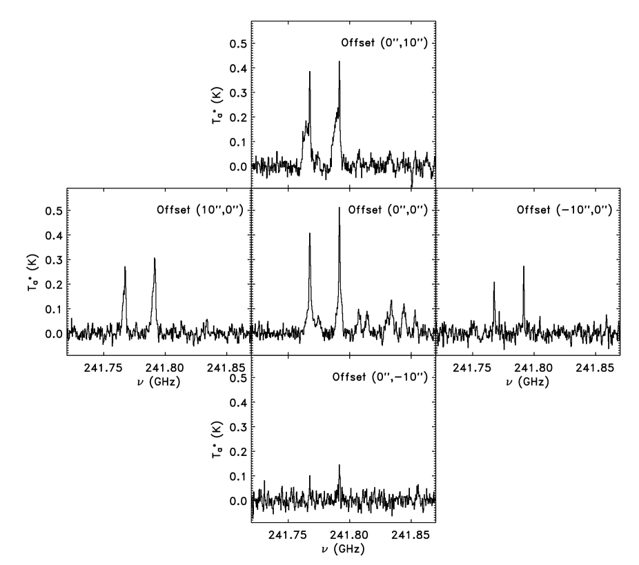
Figure 4: As in Fig. 3 for NGC1333-IRAS2. A first outflow is oriented towards north-south, and a second one towards east-west (see text).

Figure 5: Comparison between two methanol (this paper) and one formaldehyde line profiles (Paper I) from NGC1333-IRAS2 and L1448-N. The vertical dashed line indicates the $v_{\mathrm{lsr}}$ of the sources.

4 Modeling

4.1 Rotational diagrams

Rough estimates of the kinetic temperatures and column densities have been obtained from the rotational diagrams of each source (Fig. 6). The observations are reasonably well fitted by a straight line, with some scattering, which is probably due to opacity and non-LTE effects. No differences are observed between the JCMT and IRAM-30m observations, despite the different beam widths of the two instruments.

The derived rotational temperature and column densities are summarized in Table 2. The derived column densities range between 0.5 and $8\times 10^{14}\ \mathrm{cm}^{-2}$. For most of the sources, rotational temperatures are around 30 K. Two notable exceptions are NGC1333-IRAS2 and IRAS16293-2422, whose rotational temperatures are about 100 and 85 K respectively. That the temperatures are larger in these two sources is not a surprise, for they are the only two sources where several lines with high level energy are detected, despite the fact that lines with low level energy are not much brighter than in the other sources. It is therefore very likely that the observed methanol lines in NGC1333-IRAS2 and IRAS16293-2422 originate in the hot region of the envelope.

Rotational temperatures should, however, be considered with some caution, because they may not reflect the actual kinetic temperatures. As noted by Bachiller et al. (1995) and Buckle & Fuller (2002), methanol can be very sub-thermally populated in interstellar conditions, and the rotational temperature derived from methanol rotational diagram analysis could be significantly lower than the kinetic temperature. Part of the differences seen from one source to an other could be due to differences in excitation. In the next section, a more detailed analysis including non-LTE excitation is developed, in order to take these effects into account.

Figure 6: Rotational diagrams of CH₃OH lines. Detected lines are marked by circles with error bars. Arrows indicate $2\sigma$ upper limits.

Table 2: Results from the rotational diagrams.

Source	$T_{\mathrm{rot}}$	$N(\mathrm{CH}_{3}\mathrm{OH})$
	(K)	($\mathrm{cm}^{-2}$)
NGC1333-IRAS4A	24 $\pm$ 2	$(5.1\pm 1.0)\times 10^{14}$
NGC1333-IRAS4B	34 $\pm$ 4	$(3.5\pm 0.8)\times 10^{14}$
NGC1333-IRAS2	101 $\pm$ 16	$(3.4\pm 0.6)\times 10^{14}$
L1448-MM	46 $\pm$ 10	$(8.8\pm 2.4)\times 10^{13}$
L1448-N	19 $\pm$ 3	$(9.4\pm 3.6)\times 10^{13}$
L1157-MM	33 $\pm$ 25	$(5.3\pm 4.9)\times 10^{13}$
IRAS16293-2422	84 $\pm$ 8	$(8.1\pm 0.9)\times 10^{14}$

4.2 Jump models

To determine more precisely the methanol abundance in the envelopes, a detailed 1-D radiative transfer model has been developed. The model uses the escape probability formalism, and has been presented in detail in Paper I. The energy levels and Einstein coefficients were taken from the Cologne Molecular Database Spectroscopy (Müller et al. 2001). CH₃OH collisional rates with para H₂ from Pottage et al. (2004) were used. The threefold hindering potential of the molecule leads to the formation of $A$ and $E$ symmetry states (see Appendix A). Because no radiative or collisional transitions are possible between the $E$ and $A$ symmetry species, these were modelled separately. The first 100 levels were considered for each symmetry of the molecule. Finally, only the ground torsional vibration state ($v_{t}$=0) was considered. The first excited state of the torsional vibration ($v_{t}$=1) is about 200 cm^-1 ($\sim$ 290 K) above the ground state. Levels with $v_{t}$=1 might be excited and decay to the torsional vibration ground state, but in a higher rotational state. However, radiative excitation due to the dust is generally inefficient, and, for the density and temperature ranges present here, collisional excitation to those levels is expected to be negligible (Schöier et al. 2002).

The envelopes have been assumed to be spherically symmetric, and power-law density profiles have been adopted. The index of the power-law density profiles and the dust temperature profiles were taken from Jørgensen et al. (2002) and Paper I. The methanol abundance profile has been supposed to follow a step function (Paper I). The abundance is set to a constant value $X_{\mathrm{out}}$, in the outer cold part of the envelope. This abundance jumps to a $X_{\mathrm{in}}$ value in the inner and hotter part of the envelope, because of the evaporation of the grain mantles.

The adopted “jump” abundance profiles may seem simplistic, because other physical and chemical processes in the envelope could lead to more complex abundance profiles. It has been suggested that the formaldehyde abundance in the outer envelope of L1448-C and IRAS16293-2422 follow a “drop” profile (Schöier et al. 2004). In this model, the abundance is reduced in the cold dense part of the envelope where CO is frozen out, but is undepleted in the inner region of the envelope, where T $>$ 50 K. The outer radius of the “drop” region is fixed where the density equals $10^{5}\ \mathrm{cm}^{-3}$. Support for this suggestion stems from OVRO observations, which cannot be reproduced on the short baselines by the jump scenario proposed in Paper I. Increasing the formaldehyde abundance in the outer region was found to give a better agreement with the observations.

Another possible explanation for the discrepancy between “jump” models and the OVRO observations could be that, for transitions with the lowest level energy, the clouds in which the protostars are embedded contribute significantly to the short baseline emission. This emission was not taken into account either in Paper I or in Schöier et al. (2004). Emission from the cloud would have the same effect as increasing the formaldehyde abundance in the outer envelope. Indeed, the outer radii of the “drop” region is about 5000 AU and 8 000 AU from the center for IRAS16293-2422 and L1448-MM respectively. At these radius, the temperature of the gas is only $\sim 10$ K, and the contribution of the cloud is likely to become important.

Therefore, the main difference between the “jump” and “drop” scenarios is the temperature at which the evaporation occurs in the inner region of the envelope. Schöier et al. (2004) adopted a temperature of 50 K, while a temperature of 90 K was adopted in Paper I. Methanol trapped in water ice will evaporate at the sublimation temperature of pure water ice ($\sim 90$ K). Because observations of interstellar ices suggests that CH₃OH is coexistent with H₂O in the ices (Skinner et al. 1992; Gerakines et al. 1999; Boogert et al. 2000), we have adopted 90 K for the sublimation temperature. We refer the reader to Paper I for a discussion of the effect of varying the evaporation temperature.

In principle, the evaporation temperature depends on the composition of ices. If methanol is trapped in water rich (polar) ices, the evaporation is likely to occur at the evaporation temperature of pure water ice ($\sim$ 90 K). On the other hand, if methanol is trapped in CO rich (apolar) ices, the temperature will occur at a lower temperature ($\sim$ 30 K). In this study, the methanol was assumed to be trapped mostly in water rich ices, and the evaporation temperature was therefore assumed to be 90 K. We refer the reader to Paper I for a discussion of the effect of varying the evaporation temperature.

The values of $X_{\mathrm{out}}$ and $X_{\mathrm{in}}$ were determined by running a grid of 10 $\times$ 10 models for each source, with the abundances ranging from 10^-12 to 10^-4. The best fit parameters were then determined by computing the $\chi^{2}$ at each point of the grid. The grid was eventually refined around the best fit solutions to determine more precisely the abundances. Fig. 7 present the $\chi^{2}$ maps obtained for each source. The figure indicates the 1, 2 and 3$\sigma$ confidence levels, the number of lines considered, as well as the reduced $\chi^{2}$ for the best fit model. The best fit models reproduce the observations quite well, with the reduced $\chi^{2}$ ranging from 0.5 to 3.5. The abundances obtained are presented in Table 3.

The methanol abundance in the outer part of the envelope ranges from $3\times 10^{-10}$ to $2\times 10^{-9}$. The inner abundance varies much more from one source to the other. In two sources of our sample, NGC1333-IRAS2 and IRAS16293-2422, the observations can only be reproduced by our model if there are jumps in the abundances. The inner abundances are $3\times 10^{-7}$ and $1\times 10^{-7}$ respectively, i.e. a factor 100 and 200 larger than in the outer envelope. We note that IRAS16293-2422 abundances are in good agreement with those obtained previously by Schöier et al. (2002). In NGC1333-IRAS4B and L1448-MM, there is weak evidence for abundance jumps ($1\sigma$). In these sources, the inner abundance jumps to $7\times 10^{-7}$ and $5\times 10^{-7}$ respectively, i.e. a factor about 300 larger than in the outer cold part of the envelope. These values should however be treated with some caution, because of the low confidence level. In NGC1333-IRAS4A, L1448-N and L1157-MM, the observations are well reproduced with a constant CH₃OH abundance throughout the envelope, even if the presence of a jump up to a few $10^{-7}$ cannot be ruled out by the present observations in these sources.

Table 3: Summary of derived abundances.

Source	COa	H2COb		CH3OHc
		Outerd	Innere	Outerd	Innere
NGC1333-IRAS4A	$8\times 10^{-6}$	$2\times 10^{-10}$	$2\times 10^{-8}$	$7\times 10^{-10}$	$<1\times 10^{-8}$
NGC1333-IRAS4B	$1\times 10^{-5}$	$5\times 10^{-10}$	$3\times 10^{-6}$	$2\times 10^{-9}$	$7\times 10^{-7}$i
NGC1333-IRAS2	$2\times 10^{-5}$	$3\times 10^{-10}$	$2\times 10^{-7}$	$1\times 10^{-9}$	$3\times 10^{-7}$
L1448-MM	$4\times 10^{-5}$	$7\times 10^{-10}$	$6\times 10^{-7}$	$2\times 10^{-9}$	$5\times 10^{-7}$i
L1448-N	…	$3\times 10^{-10}$	$1\times 10^{-6}$	$7\times 10^{-10}$	$<4\times 10^{-7}$
L1157-MM	$6\times 10^{-6}$	$8\times 10^{-11}$	$1\times 10^{-8}$	$3\times 10^{-10}$	$<3\times 10^{-8}$
IRAS16293-2422	$3\times 10^{-5}$	$1\times 10^{-9}$	$1\times 10^{-7}$	$1\times 10^{-9}$	$1\times 10^{-7}$
L134Nd	$1\times 10^{-4}$	$2\times 10^{-8}$		$5\times 10^{-9}$
Orion hot coree	$1\times 10^{-4}$	$7\times 10^{-9}$		$1\times 10^{-7}$
High mass YSOf	$(0.3-1.7)\times 10^{-4}$	$(1-10)\times 10^{-9}$		$(0.4-24)\times 10^{-9}$	$(6-9)\times 10^{-8}$
L1157 outflowg	$1\times 10^{-4}$	$2\times 10^{-7}$		$2\times 10^{-5}$
Icesh	$(0.2-3)\times 10^{-5}$	$(1-4)\times 10^{-6}$		$(0.2-2)\times 10^{-5}$

^a From Jørgensen et al. (2004b) and Schöier et al. (2002).
^b From Paper I.
^c This study.
^d From Dickens et al. (2000) (position C).
^e From Sutton et al. (1995).
^f From van der Tak et al. (2000a, b).
^g From Bachiller & Perez Gutierrez (1997).
^h From Ehrenfreund & Charnley (2000) and Gibb et al. (2004), assuming $X(\mathrm{H}_{2}\mathrm{O})=5\times 10^{-5}$.
ⁱ $1\sigma$ confidence level only.

Figure 7: $\chi^{2}$ as a function of the inner and outer CH₃OH abundance. The contours indicate the 1, 2 and 3$\sigma$ confidence levels. The number of observed lines, $N$, are also shown, as well as the reduced $\chi^{2}$ for the best fit model.

5 Discussion

The abundance of methanol in the outer regions of Class 0 protostars is $3-20\times 10^{-10}$, a value comparable with the ones observed in cold dark clouds ($5\times 10^{-9}$, Dickens et al. 2000). Also, the observations reveal clear evidence for high methanol abundances in the envelopes of two Class 0 protostars, IRAS16293-2422 and NGC1333-IRAS2. At the two sigma level, two other protostars – NGC1333-IRAS4A and L1448-MM – also show enhanced CH₃OH abundances in the inner regions. For the other sources, the evidence is inconclusive.

The presence of large abundance jumps in the inner regions of low mass protostars is often cited as evidence for the importance of evaporation of ice mantles due to heating by the newly formed star. These ice mantles are thought to form during the preceding, cold, prestellar core phase. This scenario is supported by the detection of high deuterium fractionation in the warm gas around low mass YSOs (Ceccarelli et al. 1998; Loinard et al. 2002; Parise et al. 2002, 2004), a tell-tale sign of low temperature chemistry. The presence of complex organic molecules (e.g. CH₃OCH₃, HCOOCH₃) also shows the importance of ice evaporation, as these molecules are generally thought to form from abundant ice species through rapid reactions in the warm gas (Charnley et al. 1992; Caselli et al. 1993). Methanol plays a central role in this drive towards molecular complexity.

It is clear that the abundance of methanol in the warm inner regions of low mass protostars can provide important clues to the chemistry of regions of star formation and, in particular, to the importance of grain surface chemistry versus gas phase chemistry. In the remainder of this section, we discuss gas phase and grain surface formation routes of methanol and compare the abundances derived for the hot core regions with models predictions.

In the gas phase, the main methanol formation route is through radiative association of CH${}_{3}^{+}$ with H₂O, followed by dissociative recombination of CH₃OH${}_{2}^{+}$ (Herbst, private communication):

$$\mathrm{CH}_{3}^{+}+\mathrm{H}_{2}\mathrm{O}\rightarrow\mathrm{CH}_{3}\mathrm{OH}_{2}^{+}+h\nu$$ (1)

$$\mathrm{CH}_{3}\mathrm{OH}_{2}^{+}+e^{-}\rightarrow\mathrm{CH}_{3}\mathrm{OH}+\mathrm{H}$$ (2)

The bottleneck in this sequence is the first step, the radiative association reaction. The rate of this reaction was recently measured to be three orders of magnitude lower at 10 K than previous estimates. Using the earlier estimate, Roberts et al. (2004) predicted a methanol abundance in dense interstellar cores of 10^-8 at early times (10⁵ yr), decreasing to 10^-9 at later times (10⁷ yr). Decreasing the reaction rate by about three orders of magnitude is expected to decrease the methanol abundance by the same factor, i.e. to between 10^-12 and 10^-11.

On grain surfaces, methanol is thought to be formed by successive hydrogenation of CO (Tielens & Hagen 1982; Tielens & Allamandola 1987):

$$\mathrm{CO}\rightarrow\mathrm{HCO}\rightarrow\mathrm{H}_{2}\mathrm{CO}\rightarrow\mathrm{H}_{2}\mathrm{COH}\rightarrow\mathrm{CH}_{3}\mathrm{OH}$$ (3)

This process has been studied experimentally by Hidaka et al. (2004), and was found to be efficient forming methanol at low temperature. Theoretical models show that methanol is abundant in icy grain mantles (CH₃OH/H₂O$\sim 0.1$) when the atomic hydrogen abundance in the accreting gas is high compared to the CO abundance (Keane & Tielens 2005).

For IRAS16293-2422 and NGC1333-IRAS2, the methanol abundance in the hot core compares well with those found in hot cores associated with regions of massive star formation ($6-10\times 10^{-8}$, Sutton et al. 1995; van der Tak et al. 2000a, b) and are much higher than methanol abundances observed in cold dark clouds ($5\times 10^{-9}$, Dickens et al. 2000). In contrast, much higher methanol abundances are associated with the outflows in the regions of low mass star formation, L1157-MM and NGC1333-IRAS2 ($2\times 10^{-5}$ and $2\times 10^{-6}$ respectively, Bachiller & Perez Gutierrez 1997; Bachiller et al. 1998). Likewise, cold ices observed along the line of sight towards high mass and low mass protostars have methanol abundances ($0.2-2\times 10^{-5}$) which are two orders of magnitude larger than observed in hot cores (Allamandola et al. 1992; Gibb et al. 2004; Pontoppidan et al. 2003, 2004). Lines of sight towards background stars on the other hand have much lower methanol ice abundances (Chiar et al. 1996, $<5\times 10^{-6}$, ).

It was realized more than a decade ago that the methanol abundances observed in the hot core associated with low and high mass protostars, interstellar ices and YSO outflows pose grave challenges to gas phase models for the formation of methanol (e.g.  Menten et al. 1988). Adopting the new rate for the radiative association rate, gas phase models fall short by four orders of magnitude. Indeed, this is one (additional) reason why the high methanol abundances in the warm gas are generally thought to reflect release into the gas phase of grain mantle species in the inner region of the envelope, either due to thermal evaporation as a result of the heating by the protostar, or due to grain mantle sputtering by the outflow. As discussed previously, our maps suggest that the methanol lines with the highest level energy do not spatially correspond to the outflow emission, but are rather peaked on the central source. Together with the small line width, this suggests that this emission originates in the hot core where grain mantles evaporate completely when the dust temperature exceeds 90 K. A similar conclusion was reached for the high H₂CO abundances observed in these same sources (Paper I). Recently, Schöier et al. (2004) investigated the origin of H₂CO abundance enhancement, using interferometric observations of IRAS16293-2422 and L1448-MM. Their maps reveals a compact emission region and small line widths and are not associated with the outflows. They conclude that these enhancements originate from thermal evaporation of the grain mantles, as claimed in Paper I. Further support for the thermal evaporation thesis is provided by the interferometric images of complex organic molecules in IRAS16293-2422, which show compact emission around the two protostars of the binary system, on scales smaller than 1” (Kuan et al. 2004; Bottinelli et al. 2004b). Here, we conclude that the scenario is very likely the same for both methanol and formaldehyde.

If the abundances observed in the hot cores of protostars are due to grain mantle evaporation, they should reflect the grain mantle composition. The observed discrepancy in the ice ($0.2-2\times 10^{-5}$) and hot core methanol abundances ($1-7\times 10^{-7}$) is then somewhat discomforting. Possibly, ice mantles are only partially released into the gas phase in these regions or the gas phase of hot cores is more heavily processed by gas phase reactions than realized before (Charnley et al. 1992). Such a partial release of ice mantles may result from small differences in temperatures between different size grains (e.g. , smaller grains or graphitic grains might be slightly warmer than larger silicate grains). Typically, a 10% difference in temperature can cause a factor 5 difference in the evaporation rate of ice mantles under interstellar conditions. Of course, within this scenario, this would imply that these warmer grains represent only a small fraction of the total ice reservoir. For shocks, partial release of the ice mantles may be a natural outcome of the sputtering in low velocity shocks.

The grain mantle scenario can be further tested by considering observed abundance ratios, involving CH₃OH, H₂CO and CO rather than absolute abundances. Of course, such a comparison inherently assumes that these species evaporate simultaneously. For traces of CO, CH₃OH and H₂CO mixed into a H₂O-rich ice, evaporation will be domainted by the evaporation of the main component. However, some of the solid CO may not be coexisting with the H₂O-rich ice mantle (Tielens et al. 1991; Chiar et al. 1998; Pontoppidan et al. 2003) and this rather volatile ice component will evaporate more readily (Sandford & Allamandola 1993). These uncertainties have to be kept in mind in the subsequent discussion.

The formation of formaldehyde and methanol from CO and H accreted onto grain surfaces has recently been studied theoretically by Keane & Tielens (2005). In their model, the formaldehyde and methanol abundances produced depend on two parameters: the density and the ratio $P$ of the probability of H to react with CO relative to H₂CO (see Eq. 3). Fig. 8 presents the abundances ratio of H₂CO and CO relative to CH₃OH predicted by the model and observed in various environments. First, we note that the H₂CO/CH₃OH and CO/CH₃OH abundance ratios observed in the warm gas around low mass protostars are somewhat higher than those observed in ices (Fig. 8). Both sets of observations are well fitted by the model, for an adopted $P$ of 1. The differences between the low mass hot cores and the high mass ices reflect a difference in the density during accretion, 10⁵ versus $10^{4}$ cm^-3, respectively. This value for $P$ is in good agreement with recent experimental estimates (Hidaka et al. 2004). We note that for a density of $10^{5}$ cm^-3, the calculated CH₃OH/H₂O ratio is $10^{-3}$. This is about a factor of 40 less than the observed CH₃OH/H₂O ratio in IRAS16293-2422 (assuming a water abundance of $3\times 10^{-6}$, Ceccarelli et al. 2000a). Higher abundance ratios are obtained when accretion occurs at lower densities where the atomic H abundance is higher (Keane & Tielens 2005). Indeed, both the observed absolute and relative abundances of these species are in good agreement with the ice observations towards high mass protostars for a density of 10⁴ cm^-3 at the time of formation (Keane & Tielens 2005).

We can also compare the observed abundance ratios in low mass hot cores with those observed in high mass hot cores (Fig. 8). This comparison reveals that relative to CH₃OH, the CO abundance is typically enhanced by an order of magnitude while the H₂CO abundance is typically less by a factor 3 in the latter compared to the former. As already noted by Keane & Tielens (2005), the hot core composition in regions of massive star formation are quite different from those observed in the ices towards the same type of objects (cf. Fig. 8). Possibly, the composition of the hot core has already been substantially altered from that of the evaporating ices by reactions in the warm gas (Keane & Tielens 2005). Hot core chemistry models predict that the abundance of H₂CO decreases before CH₃OH (Charnley et al. 1992), so the H₂CO over CH₃OH ratio is expected to decrease with time. Hence, the points in Fig 8 are expected to shift from the calculated grain surface chemistry curves to the lower right corner with time. From this perspective, the differences in the abundance ratios between high and low mass hot cores could therefore be interpreted in terms of different ages for these two kind of regions: high mass hot cores are typically older than low mass hot core. Gas phase chemistry calculations are needed to confirm this scenario.

Summarizing this discussion, we conclude that current gas phase chemistry models fail to reproduce the observed methanol abundances by many orders of magnitude. Based upon recent experimental and theoretical studies, good agreement is obtained between the observations and grain surface chemistry models in terms of relative abundance ratios of CH₃OH, H₂CO and CO. However, reproduction of absolute abundances seems to be more troublesome, perhaps pointing towards the presence of multiple ice components and for selective partial evaporation. While this comparison presents, at the moment, mixed results, further observational studies of these and related species, in combination with laboratory studies and theoretical models, promises the opportunity of developing a chemical clock which can “time” the star formation process.

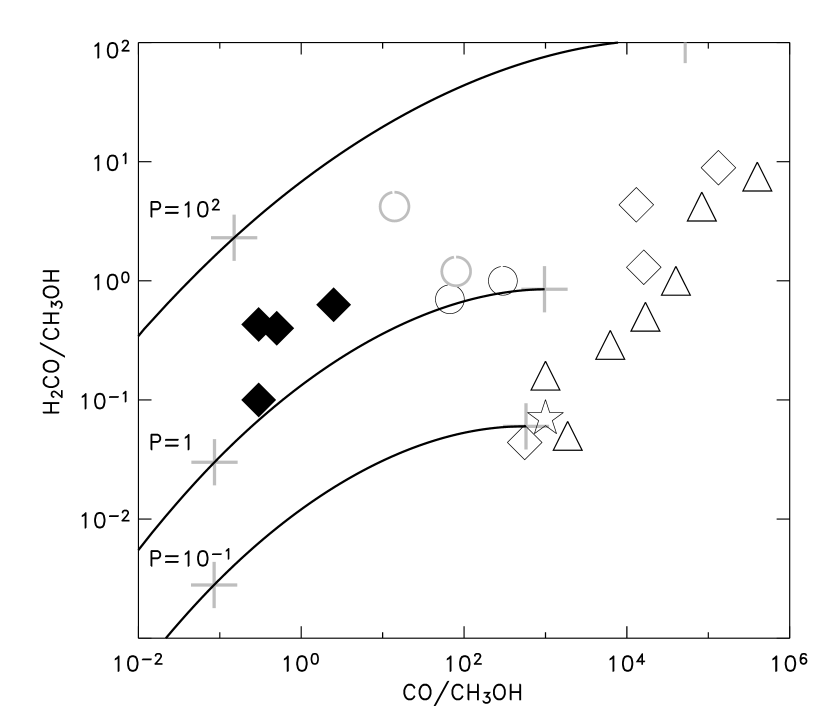
Figure 8: Abundances ratio of H₂CO and CO relative to CH₃OH. The curves show the grain chemistry model predictions for different ratio of the probability $P$ of H to react with CO relative to H₂CO. Along each curve, the density increases. The crosses denote densities of 10⁴ and 10⁵ cm^-3. Black diamonds indicates observed ice abundances towards a number of embedded young stellar objects (Keane & Tielens 2005). Open diamonds represent the gas phase abundances observed in the same objects. The star denotes the gas phase composition of the Orion hot core (Sutton et al. 1995). The open circles indicate gas phase observations of low mass protostars (this study). Black circles represent IRAS16293-2422 and NGC1333-IRAS2, for which the jumps detections are firm, while grey circles represent NGC1333-IRAS4B and L1448-MM. The triangles indicate the observed gas phase abundances towards high mass YSO (van der Tak et al. 2000a, b). Adapted from Keane & Tielens (2005).

6 Conclusions

Methanol lines observations of a sample of Class 0 protostars have been presented. Using a detailed 1-D radiative transfer model, the methanol abundance profiles have been derived and compared with chemical scenarios of the formation of this molecule. Our main conclusions are:

1. The methanol abundances in the outer cold envelopes ($<$ 90 K) are 3-20 $\times$ 10^-10, a comparable value with the ones observed in cold dark clouds.

2. Constant abundance models fail to reproduce the observations in two sources of our sample, IRAS16293-2422 and NGC1333-IRAS2. A jump at the radius where the temperature reaches 90 K has to be included in order to reproduce the observations. In two other sources, NGC1333-IRAS4B and L1448-MM, jumps in the abundance are also detected, but at a lower confidence level. In the three remaining sources, NGC1333-IRAS4A, L1448-N and L1157-MM, the observations are well reproduced by a constant abundance model, but the presence of a jump in the abundance cannot be ruled out.

3. In the sources where abundances jumps are detected, the abundance in the inner hot region ($>$ 90 K) are 1-7 $\times$ 10^-7, i.e. about two orders of magnitude larger than in cold dark cloud. The abundances in these hot cores compare well with those derived for the Orion hot core, as well as in the inner region of high mass YSO.

4. We have compared the observed methanol abundances with gas phase and grain surface chemistry models. Gas phase chemistry models predict methanol abundances (10^-11) much lower than observed in these hot cores. Grain surface chemistry models provide good agreement with the observed abundance ratios involving CH₃OH, H₂CO, and CO. However, absolute abundances are more difficult to reproduce and may point towards the presence of multiple ice components and the effects of difference in volatility between different ices species.

Table 4: Lines intensities and width for methanol transitions in NGC1333-IRAS4A.

Transition	E$\mathrm{up}$	$\nu$	$\int{T_{\mathrm{mb}}\,dv}$	$\Delta v$	Telescope	HPBW
	(K)	(GHz)	($\mathrm{K}\,\mathrm{km}\,\mathrm{s}^{-1}$)	($\mathrm{km}\,\mathrm{s}^{-1}$)		($\arcsec$)
50-40 E+	48.0	241.700	1.70 $\pm$ 0.41	2.7 $\pm$ 0.4	IRAM-30m	10
51-41 E-	40.5	241.767	4.63 $\pm$ 0.87	2.9 $\pm$ 0.2	IRAM-30m	10
50-40 A+	34.8	241.791	7.46 $\pm$ 1.40	3.7 $\pm$ 0.2	IRAM-30m	10
54-44 A±	115.2	241.806	$<$ 0.21	…	IRAM-30m	10
54-44 E-	122.8	241.813	$<$ 0.21	…	IRAM-30m	10
54-44 E+	135.8	241.829	$<$ 0.21	…	IRAM-30m	10
53-43 A±	84.7	241.832	$<$ 0.21	…	IRAM-30m	10
52-42 A-a	72.6	241.842	$<$ 0.21	…	IRAM-30m	10
53-43 E-	97.6	241.852	$<$ 0.21	…	IRAM-30m	10
51-41 E+	55.9	241.879	$<$ 0.21	…	IRAM-30m	10
52-42 A+	72.6	241.887	$<$ 0.21	…	IRAM-30m	10
71-61 E-	70.6	338.345	6.71 $\pm$ 2.08	8.1 $\pm$ 0.1d	JCMT	13
70-60 A+b	65.1	338.409	7.95 $\pm$ 2.45	8.0 $\pm$ 0.8d	JCMT	13
76-66 E-	254.7	338.431	$<$ 0.06	…	JCMT	13
76-66 A±	258.9	338.442	$<$ 0.06	…	JCMT	13
75-65 E-	189.2	338.457	0.03 $\pm$ 0.04	1.1 $\pm$ 1.3	JCMT	13
75-65 E+	206.1	338.475	$<$ 0.06	…	JCMT	13
75-65 A±	203.0	338.486	$<$ 0.06	…	JCMT	13
74-64 E-	153.1	338.504	$<$ 0.06	…	JCMT	13
72-62 A-c	102.8	338.513	0.46 $\pm$ 0.22	6.9 $\pm$ 1.4d	JCMT	13
74-64 E+	166.0	338.530	$<$ 0.06	…	JCMT	13
73-63 A±	114.9	338.541	0.75 $\pm$ 0.27	7.4 $\pm$ 0.5d	JCMT	13
73-63 E-	127.9	338.560	$<$ 0.06	…	JCMT	13
73-63 E+	112.8	338.583	0.14 $\pm$ 0.07	3.1 $\pm$ 0.9d	JCMT	13
71-61 E+	86.1	338.615	1.40 $\pm$ 0.47	7.6 $\pm$ 0.3d	JCMT	13
72-62 A+	102.8	338.640	0.29 $\pm$ 0.13	6.5 $\pm$ 1.1d	JCMT	13

^a Blended with 5₃-4₃ E⁺.
^b Blended with 7₆-6₆ E⁺.
^c Blended with 7₄-6₄ A^±.
^d Uncertain flux because of outflow contamination

Table 5: As in Table 4 for NGC1333-IRAS4B.

Transition	E$\mathrm{up}$	$\nu$	$\int{T_{\mathrm{mb}}\,dv}$	$\Delta v$	Telescope	HPBW
	(K)	(GHz)	($\mathrm{K}\,\mathrm{km}\,\mathrm{s}^{-1}$)	($\mathrm{km}\,\mathrm{s}^{-1}$)		($\arcsec$)
50-40 E+	48.0	241.700	1.56 $\pm$ 0.50	1.2 $\pm$ 0.4	IRAM-30m	10
51-41 E-	40.5	241.767	2.39 $\pm$ 0.53	1.1 $\pm$ 0.1	IRAM-30m	10
50-40 A+	34.8	241.791	3.74 $\pm$ 0.77	1.3 $\pm$ 0.1	IRAM-30m	10
54-44 A±	115.2	241.806	$<$ 0.30	…	IRAM-30m	10
54-44 E-	122.8	241.813	$<$ 0.30	…	IRAM-30m	10
54-44 E+	135.8	241.829	$<$ 0.30	…	IRAM-30m	10
53-43 A±	84.7	241.832	$<$ 0.30	…	IRAM-30m	10
52-42 A-a	76.8	241.842	$<$ 0.30	…	IRAM-30m	10
53-43 E-	97.6	241.852	$<$ 0.30	…	IRAM-30m	10
51-41 E+	55.9	241.879	$<$ 0.30	…	IRAM-30m	10
52-42 A+	72.6	241.887	$<$ 0.30	…	IRAM-30m	10
71-61 E-	70.6	338.345	5.27 $\pm$ 1.66	3.7 $\pm$ 0.1	JCMT	13
70-60 A+b	65.1	338.409	5.78 $\pm$ 1.81	3.4 $\pm$ 0.6	JCMT	13
76-66 E-	254.7	338.431	$<$ 0.08	…	JCMT	13
76-66 A±	258.9	338.442	$<$ 0.08	…	JCMT	13
75-65 E-	189.2	338.457	$<$ 0.08	…	JCMT	13
75-65 E+	206.1	338.475	$<$ 0.08	…	JCMT	13
75-65 A±	203.0	338.486	$<$ 0.08	…	JCMT	13
74-64 E-	153.1	338.504	$<$ 0.08	…	JCMT	13
72-62 A-c	131.2	338.513	0.76 $\pm$ 0.29	4.7 $\pm$ 0.5	JCMT	13
74-64 E+	166.0	338.530	$<$ 0.08	…	JCMT	13
73-63 A±	114.9	338.541	1.29 $\pm$ 0.47	5.3 $\pm$ 0.4	JCMT	13
73-63 E-	127.9	338.560	$<$ 0.08	…	JCMT	13
73-63 E+	112.8	338.583	0.30 $\pm$ 0.19	3.0 $\pm$ 1.0	JCMT	13
71-61 E+	86.1	338.615	1.60 $\pm$ 0.61	4.2 $\pm$ 0.4	JCMT	13
72-62 A+	102.8	338.640	0.52 $\pm$ 0.27	4.0 $\pm$ 1.1	JCMT	13

^a Blended with 5₃-4₃ E⁺.
^b Blended with 7₆-6₆ E⁺.
^c Blended with 7₄-6₄ A^±.

Table 6: As in Table 4 for NGC1333-IRAS2.

Transition	E$\mathrm{up}$	$\nu$	$\int{T_{\mathrm{mb}}\,dv}$	$\Delta v$	Telescope	HPBW
	(K)	(GHz)	($\mathrm{K}\,\mathrm{km}\,\mathrm{s}^{-1}$)	($\mathrm{km}\,\mathrm{s}^{-1}$)		($\arcsec$)
50-40 E+	48.0	241.700	0.89 $\pm$ 0.34	2.9 $\pm$ 0.8	IRAM-30m	10
51-41 E-	40.5	241.767	1.67 $\pm$ 0.41	2.4 $\pm$ 0.3	IRAM-30m	10
50-40 A+	34.8	241.791	1.74 $\pm$ 0.40	2.0 $\pm$ 0.2	IRAM-30m	10
54-44 A±	115.2	241.806	0.54 $\pm$ 0.20	3.5 $\pm$ 1.0	IRAM-30m	10
54-44 E-	122.8	241.813	0.47 $\pm$ 0.19	3.3 $\pm$ 1.0	IRAM-30m	10
54-44 E+	135.8	241.829	0.42 $\pm$ 0.22	3.4 $\pm$ 1.3	IRAM-30m	10
53-43 A±	84.7	241.832	0.74 $\pm$ 0.27	3.2 $\pm$ 0.8	IRAM-30m	10
52-42 A-a	76.8	241.842	0.75 $\pm$ 0.22	3.6 $\pm$ 0.5	IRAM-30m	10
53-43 E-	97.6	241.852	0.39 $\pm$ 0.16	2.8 $\pm$ 0.9	IRAM-30m	10
51-41 E+	55.9	241.879	1.00 $\pm$ 0.26	3.5 $\pm$ 0.5	IRAM-30m	10
52-42 A+	72.6	241.887	0.63 $\pm$ 0.18	2.7 $\pm$ 0.5	IRAM-30m	10
71-61 E-	70.6	338.345	1.59 $\pm$ 0.59	5.9 $\pm$ 0.5d	JCMT	13
70-60 A+b	65.1	338.409	1.89 $\pm$ 0.68	6.5 $\pm$ 0.5d	JCMT	13
76-66 E-	254.7	338.431	0.27 $\pm$ 0.14	3.0 $\pm$ 0.8	JCMT	13
76-66 A±	258.9	338.442	0.13 $\pm$ 0.12	3.2 $\pm$ 2.4	JCMT	13
75-65 E-	189.2	338.457	0.27 $\pm$ 0.19	3.1 $\pm$ 2.0	JCMT	13
75-65 E+	206.1	338.475	0.27 $\pm$ 0.18	2.7 $\pm$ 1.0	JCMT	13
75-65 A±	203.0	338.486	0.29 $\pm$ 0.20	3.0 $\pm$ 1.7	JCMT	13
74-64 E-	153.1	338.504	0.37 $\pm$ 0.22	3.4 $\pm$ 1.3	JCMT	13
72-62 A-c	131.2	338.513	0.40 $\pm$ 0.23	3.2 $\pm$ 1.3	JCMT	13
74-64 E+	166.0	338.530	0.43 $\pm$ 0.24	3.2 $\pm$ 1.1	JCMT	13
73-63 A±	114.9	338.541	0.71 $\pm$ 0.34	4.8 $\pm$ 1.0	JCMT	13
73-63 E-	127.9	338.560	0.33 $\pm$ 0.20	3.2 $\pm$ 0.8	JCMT	13
73-63 E+	112.8	338.583	0.41 $\pm$ 0.22	3.1 $\pm$ 0.9	JCMT	13
71-61 E+	86.1	338.615	0.67 $\pm$ 0.33	4.2 $\pm$ 1.1	JCMT	13
72-62 A+	102.8	338.640	0.37 $\pm$ 0.19	2.6 $\pm$ 0.7	JCMT	13

^a Blended with 5₃-4₃ E⁺.
^b Blended with 7₆-6₆ E⁺.
^c Blended with 7₄-6₄ A^±.
^d Uncertain flux because of outflow contamination

Table 7: As in Table 4 for L1448-MM.

Transition	E$\mathrm{up}$	$\nu$	$\int{T_{\mathrm{mb}}\,dv}$	$\Delta v$	Telescope	HPBW
	(K)	(GHz)	($\mathrm{K}\,\mathrm{km}\,\mathrm{s}^{-1}$)	($\mathrm{km}\,\mathrm{s}^{-1}$)		($\arcsec$)
50-40 E+	48.0	241.700	0.30 $\pm$ 0.15	1.3 $\pm$ 0.1	IRAM-30m	10
51-41 E-	40.5	241.767	0.70 $\pm$ 0.14	1.2 $\pm$ 0.1	IRAM-30m	10
50-40 A+	34.8	241.791	0.93 $\pm$ 0.17	1.1 $\pm$ 0.1	IRAM-30m	10
54-44 A±	115.2	241.806	$<$ 0.05	…	IRAM-30m	10
54-44 E-	122.8	241.813	$<$ 0.05	…	IRAM-30m	10
54-44 E+	135.8	241.829	$<$ 0.05	…	IRAM-30m	10
53-43 A±	84.7	241.832	$<$ 0.05	…	IRAM-30m	10
52-42 A-a	76.8	241.842	0.26 $\pm$ 0.07	3.5 $\pm$ 0.6	IRAM-30m	10
53-43 E-	97.6	241.852	0.25 $\pm$ 0.07	2.0 $\pm$ 0.4	IRAM-30m	10
51-41 E+	55.9	241.879	0.32 $\pm$ 0.08	1.8 $\pm$ 0.3	IRAM-30m	10
52-42 A+	72.6	241.887	$<$ 0.05	…	IRAM-30m	10
71-61 E-	70.6	338.345	0.60 $\pm$ 0.36	7.5 $\pm$ 2.5	JCMT	13
70-60 A+b	65.1	338.409	0.54 $\pm$ 0.24	5.9 $\pm$ 1.0	JCMT	13
76-66 E-	254.7	338.431	$<$ 0.11	…	JCMT	13
76-66 A±	258.9	338.442	$<$ 0.11	…	JCMT	13
75-65 E-	189.2	338.457	$<$ 0.11	…	JCMT	13
75-65 E+	206.1	338.475	$<$ 0.11	…	JCMT	13
75-65 A±	203.0	338.486	$<$ 0.11	…	JCMT	13
74-64 E-	153.1	338.504	$<$ 0.11	…	JCMT	13
72-62 A-c	131.2	338.513	$<$ 0.11	…	JCMT	13
74-64 E+	166.0	338.530	$<$ 0.11	…	JCMT	13
73-63 A±	114.9	338.541	$<$ 0.11	…	JCMT	13
73-63 E-	127.9	338.560	$<$ 0.11	…	JCMT	13
73-63 E+	112.8	338.583	$<$ 0.11	…	JCMT	13
71-61 E+	86.1	338.615	0.30 $\pm$ 0.19	7.9 $\pm$ 2.7	JCMT	13
72-62 A+	102.8	338.640	$<$ 0.11	…	JCMT	13

^a Blended with 5₃-4₃ E⁺.
^b Blended with 7₆-6₆ E⁺.
^c Blended with 7₄-6₄ A^±.

Table 8: As in Table 4 for L1448-N.

Transition	E$\mathrm{up}$	$\nu$	$\int{T_{\mathrm{mb}}\,dv}$	$\Delta v$	Telescope	HPBW
	(K)	(GHz)	($\mathrm{K}\,\mathrm{km}\,\mathrm{s}^{-1}$)	($\mathrm{km}\,\mathrm{s}^{-1}$)		($\arcsec$)
50-40 E+	48.0	241.700	0.39 $\pm$ 0.15	1.2 $\pm$ 0.4	IRAM-30m	10
51-41 E-	40.5	241.767	1.00 $\pm$ 0.20	1.1 $\pm$ 0.1	IRAM-30m	10
50-40 A+	34.8	241.791	1.33 $\pm$ 0.25	1.3 $\pm$ 0.1	IRAM-30m	10
54-44 A±	115.2	241.806	$<$ 0.05	…	IRAM-30m	10
54-44 E-	122.8	241.813	$<$ 0.05	…	IRAM-30m	10
54-44 E+	135.8	241.829	$<$ 0.05	…	IRAM-30m	10
53-43 A±	84.7	241.832	$<$ 0.05	…	IRAM-30m	10
52-42 A-a	76.8	241.842	$<$ 0.05	…	IRAM-30m	10
53-43 E-	97.6	241.852	$<$ 0.05	…	IRAM-30m	10
51-41 E+	55.9	241.879	0.26 $\pm$ 0.09	2.6 $\pm$ 0.6	IRAM-30m	10
52-42 A+	72.6	241.887	$<$ 0.05	…	IRAM-30m	10
71-61 E-	70.6	338.345	0.38 $\pm$ 0.18	1.8 $\pm$ 0.3	JCMT	13
70-60 A+b	65.1	338.409	0.48 $\pm$ 0.21	2.0 $\pm$ 0.3	JCMT	13
76-66 E-	254.7	338.431	$<$ 0.06	…	JCMT	13
76-66 A±	258.9	338.442	$<$ 0.06	…	JCMT	13
75-65 E-	189.2	338.457	$<$ 0.06	…	JCMT	13
75-65 E+	206.1	338.475	$<$ 0.06	…	JCMT	13
75-65 A±	203.0	338.486	$<$ 0.06	…	JCMT	13
74-64 E-	153.1	338.504	$<$ 0.06	…	JCMT	13
72-62 A-c	131.2	338.513	$<$ 0.06	…	JCMT	13
74-64 E+	166.0	338.530	$<$ 0.06	…	JCMT	13
73-63 A±	114.9	338.541	0.11 $\pm$ 0.10	2.8 $\pm$ 1.6	JCMT	13
73-63 E-	127.9	338.560	$<$ 0.06	…	JCMT	13
73-63 E+	112.8	338.583	$<$ 0.06	…	JCMT	13
71-61 E+	86.1	338.615	$<$ 0.06	…	JCMT	13
72-62 A+	102.8	338.640	$<$ 0.06	…	JCMT	13

^a Blended with 5₃-4₃ E⁺.
^b Blended with 7₆-6₆ E⁺.
^c Blended with 7₄-6₄ A^±.

Table 9: As in Table 4 for L1157-MM.

Transition	E$\mathrm{up}$	$\nu$	$\int{T_{\mathrm{mb}}\,dv}$	$\Delta v$	Telescope	HPBW
	(K)	(GHz)	($\mathrm{K}\,\mathrm{km}\,\mathrm{s}^{-1}$)	($\mathrm{km}\,\mathrm{s}^{-1}$)		($\arcsec$)
50-40 E+	48.0	241.700	$<$ 0.07	…	IRAM-30m	10
51-41 E-	40.5	241.767	0.51 $\pm$ 0.13	1.2 $\pm$ 0.2	IRAM-30m	10
50-40 A+	34.8	241.791	0.54 $\pm$ 0.13	1.2 $\pm$ 0.2	IRAM-30m	10
54-44 A±	115.2	241.806	$<$ 0.07	…	IRAM-30m	10
54-44 E-	122.8	241.813	$<$ 0.07	…	IRAM-30m	10
54-44 E+	135.8	241.829	$<$ 0.07	…	IRAM-30m	10
53-43 A±	84.7	241.832	$<$ 0.07	…	IRAM-30m	10
52-42 A-a	76.8	241.842	$<$ 0.07	…	IRAM-30m	10
53-43 E-	97.6	241.852	$<$ 0.07	…	IRAM-30m	10
51-41 E+	55.9	241.879	$<$ 0.07	…	IRAM-30m	10
52-42 A+	72.6	241.887	$<$ 0.07	…	IRAM-30m	10
71-61 E-	70.6	338.345	$<$ 0.21	…	JCMT	13
70-60 A+b	65.1	338.409	0.41 $\pm$ 0.27	7.8 $\pm$ 3.7	JCMT	13
76-66 E-	254.7	338.431	$<$ 0.21	…	JCMT	13
76-66 A±	258.9	338.442	$<$ 0.21	…	JCMT	13
75-65 E-	189.2	338.457	$<$ 0.21	…	JCMT	13
75-65 E+	206.1	338.475	$<$ 0.21	…	JCMT	13
75-65 A±	203.0	338.486	$<$ 0.21	…	JCMT	13
74-64 E-	153.1	338.504	$<$ 0.21	…	JCMT	13
72-62 A-c	131.2	338.513	$<$ 0.21	…	JCMT	13
74-64 E+	166.0	338.530	$<$ 0.21	…	JCMT	13
73-63 A±	114.9	338.541	$<$ 0.21	…	JCMT	13
73-63 E-	127.9	338.560	$<$ 0.21	…	JCMT	13
73-63 E+	112.8	338.583	$<$ 0.21	…	JCMT	13
71-61 E+	86.1	338.615	$<$ 0.21	…	JCMT	13
72-62 A+	102.8	338.640	$<$ 0.21	…	JCMT	13

^a Blended with 5₃-4₃ E⁺.
^b Blended with 7₆-6₆ E⁺.
^c Blended with 7₄-6₄ A^±.

Table 10: As in Table 4 for IRAS16293-2422.

Transition	E$\mathrm{up}$	$\nu$	$\int{T_{\mathrm{mb}}\,dv}$	$\Delta v$	Telescope	HPBW
	(K)	(GHz)	($\mathrm{K}\,\mathrm{km}\,\mathrm{s}^{-1}$)	($\mathrm{km}\,\mathrm{s}^{-1}$)		($\arcsec$)
50-40 E+	48.0	241.700	2.67 $\pm$ 0.83	4.5 $\pm$ 1.0	JCMT	20
51-41 E-	40.5	241.767	4.36 $\pm$ 0.97	3.3 $\pm$ 0.3	JCMT	20
50-40 A+	34.8	241.791	4.91 $\pm$ 1.03	3.2 $\pm$ 0.2	JCMT	20
54-44 A±	115.2	241.806	0.72 $\pm$ 0.46	fixeda	JCMT	20
54-44 E-	122.8	241.813	$<$ 0.10	…	JCMT	20
54-44 E+	135.8	241.829	$<$ 0.10	…	JCMT	20
53-43 A±	84.7	241.832	1.99 $\pm$ 0.75	5.3 $\pm$ 1.4	JCMT	20
52-42 A-b	72.6	241.842	1.97 $\pm$ 0.77	6.3 $\pm$ 1.7	JCMT	20
53-43 E-	97.6	241.852	0.61 $\pm$ 0.44	fixeda	JCMT	20
51-41 E+	55.9	241.879	2.29 $\pm$ 0.78	4.9 $\pm$ 1.2	JCMT	20
52-42 A+	72.6	241.887	1.67 $\pm$ 0.82	7.8 $\pm$ 3.0	JCMT	20
52-42 E-	60.8	241.904	3.28 $\pm$ 0.91	4.6 $\pm$ 0.7	JCMT	20

^a Gaussian fit with a fixed line width of 5.0 km.s^-1.
^b Blended with 5₃-4₃ E⁺.

Appendix A Spectral designation

Methanol (CH₃OH) is a slightly asymmetric rotor with hindered internal rotation of the methyl (CH₃) group. The first excited state of the torsional vibration is about 200 cm^-1 above the ground state, low enough to be populated in some particular interstellar conditions (Menten et al. 1986). Energy levels are labelled by the total angular momentum $J$, its projection along the symmetry $a$-axis $k$ or $K=|k|$, the torsional vibration quantum number $v_{t}$ and the torsional sublevel quantum number $\sigma$. The threefold symmetric torsional barrier in methanol indeed leads to the existence of three torsional symmetry states, usually designated $A$, $E_{1}$ and $E_{2}$ corresponding to $\sigma=0,+1,-1$, respectively (Lees & Baker 1968). For the $E$ species, $k\geq 0$ states are degenerate with the $E_{2}$ $k\leq 0$ states, and vice versa. It is thus simplest to refer to these states as doubly degenerate states of $E$ symmetry with positive and negative values for $k$ (Lees 1973). Levels of the $A$ species are torsionally doubly degenerate but this degeneracy is lifted by the slight asymmetry of the molecule. These doublets may be labelled by the $C_{3v}$ symmetry group notation $A_{1}$ and $A_{2}$ but the most common convention is tu use the labels $A^{+}$ and $A^{-}$. Full details about notations can be found in Lees & Baker (1968). An alternate convention for labelling the $A$ symmetry states is the use of the standard asymmetric top notation $J_{K_{a}K_{c}}$, where $K_{a}$ denotes the above $K$, as done for example in the Cologne database for molecular spectroscopy (Müller et al. 2001). In this paper, the former notation is employed.