Prospects for Dark Energy Evolution:
a Frequentist Multi-Probe Approach

A major quest in cosmology is the understanding of the nature of dark energy. It is now well known that a combination of cosmological probes is required to break the underlying degeneracies on cosmological parameters. In this paper, we present a method, based on a frequentist approach, to combine probes without any prior constraints, taking full account of the correlations in the parameters. As an application, a combination of current SNIa and CMB data with an evolving dark energy component is first compared to other analyses. We emphasise the consequences of the implementation of the dark energy perturbations on the result for a time varying equation of state. The impact of future weak lensing surveys on the measurement of dark energy evolution is then studied in combination with future measurements of the cosmic microwave background and type Ia supernovae. We present the combined results for future mid-term and long-term surveys and confirm that the combination with weak lensing is very powerful in breaking parameter degeneracies. A second generation of experiment is however required to achieve a 0.1 error on the parameters describing the evolution of dark energy.

1 Introduction

Supernovae type Ia (SNIa) observations (Knop et al. SCP04 (2003), Riess et al. Riess04 (2004)) provide strong evidence that the universe is accelerating, in very good agreement with the WMAP Cosmic Microwave Background (CMB) results (Bennett et al. wmap (2003), Spergel et al. WMAPSpergel (2003)) combined with measurements of large scale structures (Hawkins et al. 2dF (2003), Tegmark et al. SDSSWMAP (2004)). The simplest way to explain the present acceleration is to introduce a cosmological constant in Einstein’s equations. Combined with the presence of Cold Dark Matter, it forms the so-called $\Lambda$CDM model. Even if this solution agrees well with current data, the measured value of the cosmological constant is very small compared to particle physics expectations of vacuum energy, requiring a difficult fine tuning. A favourite solution to this problem involves the introduction of a new component, called ”dark energy” (DE), which can be a scalar field as in quintessence models (Wetterich Wetterich (1988), Peebles & Ratra PeeblesRatra (1988)).

The most common way to study this component is to measure its ”equation of state” (EOS) parameter, defined as $w=p/\rho\,$, where $p\,$ is the pressure and $\rho\,$ the energy density of the dark energy. Most models predict an evolving equation $w(z)$. It has been shown (e.g., Maor et al. Maor (2001), Maor et al. Maor02 (2002), Virey et al. 2004a , Gerke & Efstathiou Gerke (2002)) that neglecting such evolution biases the discrimination between $\Lambda$CDM and other models. The analysis of dark energy properties needs to take time evolution (or redshift $z$ dependence) into account.

Other attractive solutions to the cosmological constant problem imply a modification of gravity (for a review, cf., e.g., Lue et al. Lue (2004), or Carroll et al. Carroll (2005) and references therein). In this case, there is no dark energy as such and thus no dark energy equation of state. In this paper, we consider only the dark energy solution, keeping in mind that Lue et al. (Lue (2004)), among others, have shown that the induced changes in the Friedmann equations could be parameterised in ways very similar to a dark energy evolving solution.

As various authors have noted (e.g., Huterer & Turner HutererTurner (2001), Weller & Albrecht WA (2002)), SNIa observations alone will not be able to distinguish between an evolving equation of state and $\Lambda$CDM. This technique indeed requires prior knowledge of the values of some parameters. In particular, the precision on the prior matter density $\Omega_{m}$ has an impact on the constraints on the time evolution of the equation of state $w$, even in the simplest flat Universe cosmology (e.g., Virey et al. 2004b ).

Extracting dark energy properties thus requires a combined analysis of complementary data sets. This can be done by combining SNIa data with other probes such as the CMB, the large scale distributions of galaxies, Lyman $\alpha$ forest data, and, in the near future, the observation of large scale structure with the Sunyaev-Zeldovich effect (SZ) (Sunyaev & Zeldovich SZ80 (1980)) or with weak gravitational lensing surveys (WL), which provide an unique method to directly map the distribution of dark matter in the universe (for reviews, cf., e.g., Bartelmann & Schneider bar99 (2001), Mellier et al. mel02 (2002); Hoekstra et al. hoe02 (2002), Refregier alexandre (2003), Heymans et al. Heymans (2005) and references therein).

Many combinations have already been performed with different types of data and procedures, (e.g., Bridle et al. Bridle (2003), Wang & Tegmark WangTegmark (2004), Tegmark et al. SDSSWMAP (2004), Upadhye et al. Upadhye (2004), Ishak Ishak (2005), Seljak et al. Seljak (2004), Corasaniti et al. Corasaniti (2004), Xia et al. ZhangXM (2004)). All studies have shown the consistency of existing data sets with the $\Lambda$CDM model and the complementarity of the different data sets in breaking degeneracies and constraining dark energy for future experiments. But the results differ by as much as 2$\sigma$ on the central values of the parameters describing an evolving equation of state.

In this paper, we have chosen three probes, which seem to best constrain the parameters of an evolving equation of state when combined, namely, SNIa, CMB and weak lensing. Considering a flat Universe, we combine the data in a coherent way, that is to say, under identical assumptions for the dark energy properties for the three probes, and we completely avoid the use of priors. This had not always been done systematically in all previous combinations. We also adopt a frequentist approach for the data combination, where the full correlations between the cosmological parameters are taken into account. This method allows us to provide, simultaneously, confidence intervals on a large number of distinct cosmological parameters. Moreover, this approach is very flexible as it is easy to add or remove parameters in contrast with other methods.

The paper is organised as follows: In Sec. 2, we describe our framework and statistical procedure, based on a frequentist approach, which can accommodate all parameters without marginalisation. For our simulation and analysis, we use the CMBEASY package for CMB (Doran CMBEASY (2003)), the Kosmoshow program for SNIa (Tilquin kosmoshow (2003)) and an extension of the calculations from Refregier et al. (2003) for weak lensing. In each case, the programs take into account the time evolution of the equation of state (cf Sec. 2.2 for details).

In Sec. 3, we apply this method to current data sets of SNIa and WMAP data. We first verify that the constraints on the cosmological parameters estimated with a Fisher matrix technique (Fisher Fisher (1935)), are consistent with those obtained with a complete error analysis. We then compare these errors with other works and discuss the differences. In particular, we discuss how the treatment of the dark energy perturbations can explain some of the differences found in the literature.

In Sec. 4, we study the statistical sensitivities of different combinations of future surveys. We simulate expectations for the ground surveys from the Canadian French Hawaii Telescope Legacy Surveys (CFHTLS) and new CMB data from Olimpo as well as the longer term Planck and SNAP space missions. For these future experiments, the results are combined with a Fisher matrix technique, compared and discussed.

Finally, our conclusions are summarised in Sec. 5.

2 Combination method

In this section, we first summarise the framework used in this paper, and describe our approach based on frequentist statistics.

2.1 Dark Energy Parametrization

The evolution of the expansion parameter is given by the Hubble parameter $H$ through the Friedmann equation

$$\left(\frac{H(z)}{H_{0}}\right)^{2}\;=\;(1+z)^{3}\,\Omega_{m}+{\rho_{X}(z)\over\rho_{X}(0)}\,\Omega_{X}+(1+z)^{2}\,\Omega_{k},\\$$ (1)

with

$${\rho_{X}(z)\over\rho_{X}(0)}\;=\;\exp\left[3\int_{0}^{z}\,\left(1+w(z^{\prime})\right)\,d\,\ln(1+z^{\prime})\right]$$ (2)

where the ratio of the dark energy density to the critical density is denoted $\Omega_{X}$ in a general model and $\Omega_{\Lambda}$ in the simplest case of a Cosmological Constant ($w=-1$). $\Omega_{M}$ is the corresponding parameter for (baryonic+cold dark) matter. Note that we have neglected the radiation component $\Omega_{R}$. The present total and curvature density parameters are $\Omega$ and $\Omega_{\kappa}=1-\Omega$, respectively. The present value of the Hubble constant is parameterised as $H_{0}=100h$ km s^-1 Mpc^-1.

As it is not possible to constrain a completely unknown functional form $w(z)$ of the time evolution of the equation of state, we adopt a parametric representation of the $z$ dependence of the equation of state. We need this parametric form to fit all the data sets over a large range of $z$: from $z\simeq 0-1$ for the SNIa and weak lensing, up to $z\simeq 1100$ for the CMB. For this purpose, we choose the parametrization proposed by Chevallier & Polarski (Polarskiparam (2001)) and Linder (LinderA (2003)) :

$$w(z)=w_{0}+{w_{a}}z/(1+z),$$ (3)

which has an adequate asymptotic behaviour. In this paper, we thus use two parameters, $w_{0}$ and $w_{a}$, to describe the time evolution of the equation of state (see justifications in Linder & Huterer  Linder05 (2005)). For this parametrization of $w(z)$, Eq. 2 reduces to:

$$\rho_{X}(z)\;=\;\rho_{X}(0)\,e^{-3w_{a}z/(1+z)}\,(1+z)^{3(1+w_{0}+w_{a})}.$$ (4)

For a constant $w\equiv w_{0}$ ($w_{a}=0$), the usual form $\rho_{X}(z)\;=\;\rho_{X}(0)\ (1+z)^{3(1+w_{0})}$ is recovered.

The comoving distance $\chi$ is defined as

$$\chi(z)=\int_{0}^{z}\,\frac{c}{H(z^{\prime})}dz^{\prime},$$ (5)

and the comoving angular-diameter distance $r(\chi)$ is equal, respectively, to $\chi$, $R_{0}sin(\chi/R_{0})$, $R_{0}\sinh(\chi/R_{0})$, for a flat, closed and open Universe where the present curvature radius of the universe is defined as $R_{0}=c/(\kappa H_{0})$ with respectively $\kappa^{2}\equiv 1$, $-\Omega_{\kappa}$, and $\Omega_{\kappa}$.

2.2 Statistical approach

Most recent CMB analysis use Markov Chains Monte Carlo simulations (Gilks et al. MCMC (1996), Christensen & Meyer MCMC_CMB (1998)) with bayesian inference. The philosophical debate between the bayesian and the frequentist statistical approaches is beyond the scope of this paper (for a comparison of the two approaches see, for instance, Feldman & Cousins Frequentist (1998) and Zech Zech (2002)). Here, we briefly review the principles of each approach.

For a given data set, the bayesian approach computes the probability distribution function (PDF) of the parameters describing the cosmological model. The bayesian probability is a measure of the plausibility of an event, given incomplete knowledge. In a second step, the bayesian constructs a ’credible’ interval, centered near the sample mean, tempered by ’prior’ assumptions concerning the mean. On the other hand, the frequentist determines the probability distribution of the data as a function of the cosmological parameters and gives a confidence level that the given interval contains the parameter. In this way, the frequentist completely avoids the concept of a PDF defined for each parameter. As the questions asked by the two approaches are different, we might expect different confidence intervals. However, the philosophical difference between the two methods should not generally lead, in the end, to major differences in the determination of physical parameters and their confidence intervals when the parameters stay in a physical region.

Our work is based on the ’frequentist’ (or ’classical’) confidence level method originally defined by Neyman (Neyman (1937)). This choice avoids any potential bias due to the choice of priors. In addition, we have also found ways to improve the calculation speed, which gives our program some advantages over other bayesian programs. Among earlier combination studies (e.g., Bridle et al. Bridle (2003), Wang & Tegmark WangTegmark (2004), Tegmark et al. SDSSWMAP (2004), Upadhye et al. Upadhye (2004), Ishak Ishak (2005), Seljak et al. Seljak (2004), Corasaniti et al. Corasaniti (2004), Xia et al. ZhangXM (2004)) only that of Upadhye et al. (Upadhye (2004)) uses also a frequentist approach.

2.2.1 Confidence levels with a frequentist approach

For a given cosmological model defined by the $n$ cosmological parameters $\theta=(\theta_{1},\ldots,\theta_{n})$, and for a data set of $N$ quantities $x=(x_{1},\ldots,x_{N})$ measured with gaussian experimental errors $\sigma_{x}=(\sigma_{1},\ldots,\sigma_{N})$, the likelihood function can be written as:

$${\cal L}(x,\sigma_{x};\theta)=\frac{1}{\sqrt{2\pi}\sigma_{i}}exp\biggl{(}-\frac{(x_{i}-x_{i,model})^{2}}{2\sigma_{i}^{2}}\biggr{)}.$$ (6)

where $x_{model}=(x_{1,model},\ldots,x_{N,model})$ is a set of corresponding model dependent values.

In the rest of this paper, we adopt a $\chi^{2}$ notation, which means that the following quantity is minimised:

$$\chi^{2}(x,\sigma_{x};\theta)=-2\ln({\cal L}(x,\sigma_{x};\theta))$$ (7)

We first determine the minimum $\chi^{2}_{0}$ of $\chi^{2}(x,\sigma_{x};\theta)$ letting free all the cosmological parameters. Then, to set a confidence level (CL) on any individual cosmological parameter $\theta_{i}$, we scan the variable $\theta_{i}$: for each fixed value of $\theta_{i}$, we minimise again $\chi^{2}(x,\sigma_{x};\theta)$ but with $n-1$ free parameters. The $\chi^{2}$ difference, $\Delta\chi^{2}(\theta_{i})$, between the new minimum and $\chi^{2}_{0}$, allows us to compute the CL on the variable, assuming that the experimental errors are gaussian,

$$1-{\rm CL}(\theta_{i})=\frac{1}{\sqrt{2^{N_{dof}}}\Gamma(N_{dof}/2)}\int_{\Delta\chi^{2}(\theta_{i})}^{\infty}e^{-t/2}t^{N_{dof}/2-1}dt$$ (8)

where $\Gamma$ is the gamma function and the number of degrees of freedom $N_{dof}$ is equal to 1. This method can be easily extended to two variables. In this case, the minimisations are performed for $n-2$ free parameters and the confidence level ${\rm CL}(\theta_{i},\theta_{j})$ is derived from Eq. 8 with $N_{dof}=2$.

By definition, this frequentist approach does not require any marginalisation to determine the sensitivity on a single individual cosmological parameter. Moreover, in contrast with bayesian treatment, no prior on the cosmological parameters is needed. With this approach, the correlations between the variables are naturally taken into account and the minimisation fit can explore the whole phase space of the cosmological parameters.

In this study, the minimisations of $\chi^{2}(x,\sigma_{x};\theta)$ are performed with the MINUIT package (James minuit (1978)). For the 9 parameter study proposed in this paper, each fit requires around 200 calculations of $\chi^{2}$. The consumed CPU-time is dominated by the computation of the angular power spectrum ($C_{\ell}$) of the CMB in CMBEASY (Doran  CMBEASY (2003)). In practice, to get the CL for one variable, as shown, for instance, in Fig. 1, the computation of the $C_{\ell}$ is done around 10000 times. The total number of calls to perform the study presented in Tab. 1, is typically 3 or 4 times smaller than the number of calls in the MCMC technique used by Tegmark et al. (SDSSWMAP (2004)). This method is very powerful for studying the impacts of the parameters: it is not costly to add or remove parameters because the number of $C_{\ell}$ computations scales with the number of parameters, in contrast with the MCMC method, which requires the generation of a new chain.

2.2.2 Combination of cosmological probes with Fisher matrices

In parallel with this frequentist approach, to study the statistical sensitivities of different combinations of future surveys, we perform a prospective analysis based on the Fisher matrix technique (Fisher Fisher (1935)). We validate this approach by comparing its estimates of the statistical errors for the current data set with those obtained with the frequentist method described above.

The statistical errors on the $n$ cosmological parameters $\theta=(\theta_{1},\ldots,\theta_{n})$ are determined by using the inverse of the covariance matrix $V$ called the Fisher matrix $F$ defined as:

$$(V^{-1})_{ij}=F_{ij}=-\frac{\partial^{2}\ln{\cal L}(x;\theta)}{\partial\theta_{i}\partial\theta_{j}},$$ (9)

where ${\cal L}(x;\theta)$ is the likelihood function depending on the $n$ cosmological parameters and a data set of $N$ measured quantities $x=(x_{1},\ldots,x_{N})$. A lower bound, and often a good estimate, for the statistical error on the cosmological parameter $\theta_{i}$ is given by $(V_{ii})^{1/2}$.

When the measurements of several cosmological probes are combined, the total Fisher matrix $F_{tot}$ is the sum of the three Fisher matrices $F_{SN}$, $F_{WL}$ and $F_{CMB}$ corresponding respectively to the SNIa, weak lensing and CMB observations. The total covariance matrix $F_{tot}^{-1}$ allows us to estimate both, the expected sensitivity on the cosmological parameters, with the diagonal terms, and the correlations between the parameters, with the off-diagonal terms. The Fisher matrices for each probe are computed as follows.

CMB: 

In the case of CMB experiments, the data set vector $x$ corresponds to the measurements of $C_{\ell}$, the angular power spectrum of the CMB from $\ell=2$ to some cutoff $\ell_{max}$. Using Eq. 9, the Fisher matrix is written as

$$(F_{CMB})_{ij}=\sum_{l=2}^{\ell_{max}}\frac{1}{\sigma_{C_{\ell}}^{2}}\cdot\frac{\partial C_{\ell}}{\partial\theta_{i}}\cdot\frac{\partial C_{\ell}}{\partial\theta_{j}}$$ (10)

where $\sigma_{C_{\ell}}$ is the statistical error on $C_{\ell}$ obtained directly from published results or estimated as (see Knox knox95 (1995)):

$$\sigma_{C_{\ell}}=\sqrt{\frac{2}{(2\ell+1)f_{sky}}}\biggl{[}C_{\ell}+(\theta_{fwhm}s)^{2}\cdot e^{\frac{\ell^{2}\theta_{fwhm}^{2}}{8\ln(2)}}\biggr{]}$$ (11)

where the second term incorporates the effects of instrumental noise and beam smearing. In Eq. 11, $\theta_{fwhm}$, $f_{sky}$, and $s$ are respectively the angular resolution, the fraction of the sky observed and the expected sensitivity per pixel.

The $C_{\ell}$ and their derivatives with respect to the various cosmological parameters are computed with CMBEASY (Doran  CMBEASY (2003)), an object oriented C++ package derived from CMBFAST (Seljak & Zaldarriaga  cmbfast (1996)).

SNIa: 

The SNIa apparent magnitudes $m$ can be expressed as a function of the luminosity distance as

$$m(z)=M_{s_{0}}+5log_{10}(D_{L})$$ (12)

where $D_{L}(z)\equiv(H_{0}/c)\;d_{L}(z)$ is the $H_{0}$-independent luminosity distance to an object at redshift $z$. The usual luminosity distance $d_{L}(z)$ is related to the comoving angular-diameter distance $r(\chi)$ by $d_{L}(z)=(1+z)\cdot r(\chi)$, with the definition of $r(\chi)$ and $\chi(z)$ given in Sec. 2.1. The normalisation parameter $M_{s_{0}}$ thus depends on $H_{0}$ and on the absolute magnitude of SNIa.

The Fisher matrix, in this case, is related to the measured apparent magnitude $m_{k}$ of each object and its statistical error $\sigma_{m_{k}}$ by

$$(F_{SN})_{ij}=\sum_{k}\frac{1}{\sigma_{m_{k}}^{2}}\cdot\frac{\partial m_{k}}{\partial\theta_{i}}\cdot\frac{\partial m_{k}}{\partial\theta_{j}}.$$ (13)

Weak lensing: 

The weak lensing power spectrum is given by (e.g., Hu & Tegmark HuTeg99 (1999), cf, Refregier alexandre (2003) for conventions)

$$C_{\ell}=\frac{9}{16}\left(\frac{H_{0}}{c}\right)^{4}\Omega_{m}^{2}\int_{0}^{\chi_{h}}d\chi\leavevmode\nobreak\ \left[\frac{g(\chi)}{ar(\chi)}\right]^{2}P\left(\frac{\ell}{r},\chi\right),$$ (14)

where $r(\chi)$ is the comoving angular-diameter distance, and $\chi_{h}$ corresponds to the comoving distance to horizon. The radial weight function $g$ is given by

$$g(\chi)=2\int_{\chi}^{\chi_{h}}d\chi^{\prime}\leavevmode\nobreak\ n(\chi^{\prime})\frac{r(\chi)r(\chi^{\prime}-\chi)}{r(\chi^{\prime})},$$ (15)

where $n(\chi)$ is the probability of finding a galaxy at comoving distance $\chi$ and is normalised as $\int d\chi\leavevmode\nobreak\ n(\chi)=1$.

The linear matter power spectrum $P(k,z)$ is computed using the transfer function from Bardeen et al. (bar86 (1986)) with the conventions of Peacock (pea97 (1997)), thus ignoring the corrections on large scales for quintessence models (Ma et al. Ma99 (1999)). The linear growth factor of the matter overdensities $\delta$ is given by the well known equation:

$$\ddot{\delta}+2H\dot{\delta}-\frac{3}{2}H^{2}\Omega_{m}(a)\delta=0,$$ (16)

where dots correspond to time derivatives, and $\Omega_{m}(a)$ is the matter density parameter at the epoch corresponding to the dimensionless scale factor $a$. This equation is integrated numerically with boundary conditions given by the matter-dominated solution, $G=\delta/a=1$ and $\dot{G}=0$, as $a\rightarrow 0$ (see eg. Linder & Jenkins LinderJenkins (2003)). We enforce the CMB normalisation of the power spectrum $P(k,0)$ at $z=0$ using the relationship between the WMAP normalisation parameter $A$ and $\sigma_{8}$ given by Hu (Hu04 (2004)). Considerable uncertainties remain for the non-linear corrections in quintessence models (cf. discussion in Hu (Hu02 (2002))). Here, we use the fitting formula from Peacock & Dodds (pea96 (1996)).

For a measurement of the power spectrum, the Fisher matrix element is defined as:

$$(F_{WL})_{ij}=\sum_{\ell}\frac{1}{\sigma_{C_{\ell}}^{2}}\frac{\partial C_{\ell}}{\partial\theta_{i}}\frac{\partial C_{\ell}}{\partial\theta_{j}},$$ (17)

where the summation is over modes $\ell$ which can be reliably measured. This expression assumes that the errors $\sigma_{C_{\ell}}$ on the lensing power spectrum are gaussian and that the different modes are uncorrelated. Mode-to-mode correlations have been shown to increase the errors on cosmological parameters (Cooray & Hu  coo01 (2001)) but are neglected in this paper.

Neglecting non-gaussian corrections, the statistical error $\sigma_{C_{\ell}}$ in measuring the lensing power spectrum $C_{\ell}$ (cf., e.g., Kaiser b13 (1998), Hu & Tegmark HuTeg99 (1999), Hu Hu02 (2002)) is given by:

$$\sigma_{C_{\ell}}=\sqrt{\frac{2}{(2l+1)f_{\rm sky}}}\left(C_{l}+\frac{\sigma_{\gamma}^{2}}{2n_{g}}\right),$$ (18)

where $f_{\rm sky}$ is the fraction of the sky covered by the survey, $n_{g}$ is the surface density of usable galaxies, and $\sigma_{\gamma}^{2}=\langle|\gamma|^{2}\rangle$ is the shear variance per galaxy arising from intrinsic shapes and measurement errors.

2.3 Cosmological parameters and models

For the studies presented in this paper, we limit ourselves to the 9 cosmological parameters: $\theta=\Omega_{b},\Omega_{m},h,n_{s},\tau,w_{0},w_{a},A$ and $M_{s_{0}}$, with the following standard definitions:
- ($\Omega_{i}$ , i=b,m) are densities for baryon and matter respectively ($\Omega_{m}$ includes both dark matter and baryons),
- $h$ is the Hubble constant in units of 100 km/s/Mpc,
- $n_{s}$ is the spectral index of the primordial power spectrum,
- $\tau$ is the reionisation optical depth,
- $A$ is the normalisation parameter of the power spectrum for CMB and weak lensing (cf Hu & Tegmark (HuTeg99 (1999)) for definitions). The matter power spectrum is normalised according to the COBE normalisation (Bunn & White BunnWhite (1997)), which corresponds to $\sigma_{8}=0.88$. This is consistent with the WMAP results (Spergel et al. WMAPSpergel (2003)) and with the average of recent cosmic shear measurements (see compilation tables in Mellier et al. mel02 (2002), Hoekstra et al. hoe02 (2002), Refregier alexandre (2003)).
- $M_{s_{0}}$ is the normalisation parameter from SNIa (cf Sec. 2.2.2),
- Dark energy is described by the $w_{0}$ parameter corresponding to the value of the equation of state at $z$=0. When the $z$ dependence of the equation of state is studied, an additional parameter $w_{a}$ is defined (cf Sec. 2.1).

The reference fiducial model of our simulation is a $\Lambda$CDM model with parameters $\Omega_{m}=0.27$, $\Omega_{b}=0.0463$, $n_{s}=0.99$, $h=0.72$, $\tau=0.066$, $A=0.86$, consistent with the WMAP experiment (see tables 1-2 in Spergel et al. WMAPSpergel (2003)). In agreement with this experiment, we assume throughout this paper that the universe is flat, i.e., $\Omega=\Omega_{m}+\Omega_{X}=1$. We also neglect the effect of neutrinos, using 3 degenerate families of neutrinos with masses fixed to 0.

In the following, we will consider deviations from this reference model. For the equation of state, we use as a reference $w_{0}=-0.95$ and $w_{a}=0$ as central values (we have not used exactly $w_{0}=-1$ to avoid transition problems in the CMB calculations). To estimate the sensitivity on the parameters describing the equation of state, we also consider two other fiducial models: a SUGRA model, with ($w_{0}=-0.8,w_{a}=0.3$) as proposed by, e.g., Weller & Albrecht (WA (2002)) to represent quintessence models, and a phantom model (Caldwell Caldwell (2002)) with ($w_{0}=-1.2,w_{a}=-0.3$).

In this analysis, the full covariance matrix on all parameters is used with no prior constraints on the parameters, avoiding biases from internal degeneracies. We have implemented the time evolving parametrization of the equation of state in simulations and analysis of the three probes we consider in this paper, i.e. CMB, SNIa and weak lensing.

3 Combination of current surveys

We first apply our statistical approach to the combination of recent SNIa and CMB data, without any external constraints or priors. The comparison of the statistical errors obtained with a global fit using this frequentist treatment, with those predicted with the Fisher matrix technique, also allows us to validate the procedure described in Sec. 2. Finally, we compare our results with other published results.

3.1 Current surveys

We use the ’Gold sample’ data compiled by Riess et al. (Riess04 (2004)), with 157 SNIa including a few at $z>1.3$ from the Hubble Space Telescope (HST GOODS ACS Treasury survey), and the published data from WMAP taken from Spergel et al. (WMAPSpergel (2003)).

We perform two distinct analyses: in the first case, the equation of state is held constant with a single parameter $w_{0}$ and we fit 8 parameters, as described in Sec. 2.2; in the second case, the $z$ dependence of the equation of state is modelled by two variables $w_{0}$ and $w_{a}$ as defined in Sec. 2.1, and we fit 9 parameters.

3.2 Results

The results of this frequentist combination of CMB and SNIa data are summarised in Tab. 1. When the equation of state is considered constant, we obtain $w_{0}=-0.92_{-0.13}^{+0.10}$ (1-$\sigma$) and the shape of the CL is relatively symmetrical around the value of $w_{0}$ obtained at the $\chi^{2}$ minimum. When a $z$ dependence is added to the equation of state, the CL is still symmetrical with $w_{0}=-1.09_{-0.15}^{+0.13}$ but $w_{a}$ becomes asymmetrical with a long tail for smaller values of $w_{a}$, as can be seen in Fig. 1. The 1-D CL for $w_{a}$ gives the resulting CL at 68%$(1\sigma)$ and 95%$(2\sigma)$: $w_{a}=0.82_{-0.26}^{+0.21}\,{}_{-0.80}^{+0.42}$.

Table 1: Results of the frequentist fit to WMAP and Riess et al. (2004) SNIa data. For the 8 parameter fit with a constant EOS, the first column gives the value of the variable at the $\chi^{2}$ minimum, with the confidence interval at 68% (1 $\sigma$), the second column shows the $1\sigma$ error computed with the Fisher matrix techniques. The third and fourth columns present the same information for the 9 parameter fit with a $z$ dependent EOS. The $1\sigma$ errors are symmetrical for all the variables except for $w_{a}$. Its error goes from ${}_{-0.26}^{+0.21}$ for CL at 68% to ${}_{-0.80}^{+0.42}$ for CL at 95% (see text).

	constant EOS		$z$ dependent EOS
	fit	$\sigma_{Fisher}$	fit	$\sigma_{Fisher}$
${\mathbf{\Omega}_{b}}$	$0.049_{-0.003}^{+0.005}$	$\pm 0.003$	$0.055_{-0.003}^{+0.003}$	$\pm 0.003$
${\mathbf{\Omega}_{m}}$	$0.29_{-0.04}^{+0.05}$	$\pm 0.04$	$0.33_{-0.04}^{+0.04}$	$\pm 0.04$
${\mathbf{h}}$	$0.69_{-0.02}^{+0.03}$	$\pm 0.03$	$0.69_{-0.02}^{+0.03}$	$\pm 0.03$
${\mathbf{n}_{S}}$	$0.97_{-0.03}^{+0.03}$	$\pm 0.03$	$0.97_{-0.03}^{+0.03}$	$\pm 0.03$
${\mathbf{\tau}}$	$0.13_{-0.04}^{+0.04}$	$\pm 0.04$	$0.14_{-0.04}^{+0.04}$	$\pm 0.04$
${\mathbf{w}_{0}}$	$-0.92_{-0.13}^{+0.10}$	$\pm 0.11$	$-1.09_{-0.15}^{+0.13}$	$\pm 0.14$
${\mathbf{w}_{a}}$	-	-	$0.82_{-0.26}^{+0.21}$	$\pm 0.25$
${\mathbf{A}}$	$0.79_{-0.07}^{+0.08}$	$\pm 0.10$	$0.80_{-0.07}^{+0.08}$	$\pm 0.10$
${\mathbf{M}_{s0}}$	$15.94_{-0.03}^{+0.03}$	$\pm 0.03$	$15.95_{-0.03}^{+0.03}$	$\pm 0.03$

Tab. 1 compares the $1\sigma$ errors obtained with the frequentist method and the errors predicted with the Fisher matrix techniques. The agreement is good, and in the remaining part of this paper, for the combination of expectations from future surveys, we will use the Fisher matrix approach.

However Upadhye et al. (Upadhye (2004)) noticed that the high redshift limit of the parametrization of the EOS plays an important role when we consider CMB data which impose $w(z\to\infty)<0$. With our choice of parametrization (see definition in Eq. 3), we get the condition $w_{0}+w_{a}<0$. When a fit solution is found close to this boundary condition, as is the case with the current data, the CL distributions are asymmetric, giving asymmetrical errors. The Fisher matrix method is not able to represent complicated 2-D CL shapes, as those shown in Fig. 2. For example, the error on $w_{a}$ increases when the $(w_{0},w_{a})$ solution moves away from the ’unphysical’ region $w_{0}+w_{a}>0$. To avoid this limitation, we will thus use fiducial values of $w_{a}$ closer to zero for the prospective studies with future surveys.

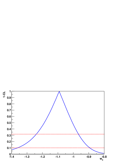
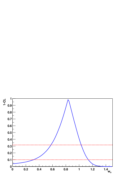
Figure 1: Confidence level (CL) plots on parameters $w_{0}$ (left) and $w_{a}$ (right), using WMAP and Riess et al. Riess04 (2004) SNIa data for a 9 parameter fit with evolving EOS. The dashed lines correspond to the 68%$(1\sigma)$ and 90%$(1.64\sigma)$ confidence intervals.

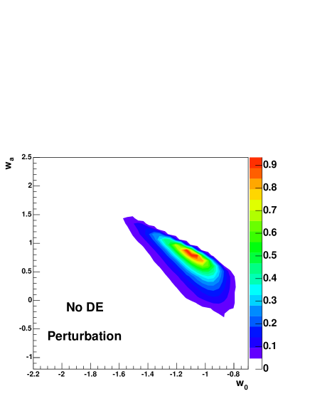
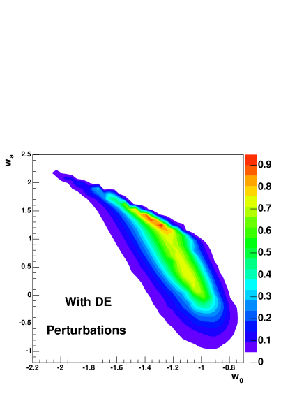
Figure 2: Confidence level contour plots with WMAP and Riess et al. Riess04 (2004) SNIa data, for the 9 parameter fit with a $z$ dependent EOS in the plane ($w_{0},w_{a}$). The plot on the left hand side corresponds to the case when we introduce no dark energy perturbation. For the plot on the right hand side, we introduce dark energy perturbations only when $w>-1$.

It is worth noting that the solution found by the fit corresponds to a value of $w$ slightly smaller than -1 for $z=0$, and a value of $w$ slightly larger than -1 for high $z$. The errors are such that the value of $w$ is compatible with -1. However, this technically means that the Universe crosses the phantom line in its evolution. This region ($w<-1$) cannot be reached by the fit, if dark energy perturbations are computed in the CMBEASY version we use. To obtain a solution and compare with other published results, we therefore probed two different conditions, both illustrated in Fig. 2.

First, we removed altogether the perturbations for the dark energy, which gives the results presented above. This allows a comparison with Seljak et al. (Seljak (2004)), who have likely removed dark energy perturbations. Their central value corresponds to $w_{0}=-0.98_{-0.37}^{+0.38}$ and $w_{a}=-0.05_{-1.13}^{+1.92}$ at 95%$(2\sigma)$. It is closer to $w=-1$ than our result and gives errors for $w_{a}$ larger than the ones we get. The comparison is however not exact, since Seljak et al. use a bayesian approach for the fits, and give results for an evolving equation of state, only for the total combination of the WMAP and SNIa data with other SDSS probes (galaxies clustering, bias, and Lyman $\alpha$ forest).

We also performed the fits, including dark energy perturbations, only when $w>-1$ (which is the default implementation in CMBFAST). Caldwell & Doran (DoranCaldwell (2005)) have argued convincingly that crossing the cosmological constant boundary leaves no distinct imprint, i.e., the contributions of $w<-1$ are negligible, because $w<-1$ dominates only at late times and dark energy does not generally give strong gravitational clustering. Our analysis, including dark energy perturbations only when $w>-1$, gives a minimum (cf. right hand side plot in Fig. 2) for $w_{0}=-1.32_{-0.19}^{+0.15}$ and $w_{a}=1.2_{-0.8}^{+0.5}$ at $1\sigma$. This is some $2\sigma$ away from the no perturbation case. We remark that these values are very close to those obtained by Upadhye et al.(Upadhye (2004)), who use a procedure similar to ours, without any marginalisation on parameters, a weak constraint $w_{0}+w_{a}\leq 0$ inside their fit. Their result, $w_{0}=-1.3_{-0.39}^{+0.34}$ and $w_{a}=1.25_{-2.17}^{+0.40}$ at 95%$(2\sigma)$, has almost the same central value as our fit, when we switch on the dark energy perturbation for $w>-1$. The errors we get are also compatible, and are much larger than in the no perturbation case.

The importance and impact of introducing dark energy perturbations has been discussed by Weller & Lewis (Weller (2003)). Their combined WMAP and SNIa analysis with a constant sound speed also gives a more negative value of $w$, when a redshift dependence is taken into account. Although Rapetti et al. (Rapetti (2004)) observe a reduced effect when they add cluster data, they still indicate a similar trend. Finally, when dark energy perturbations are included, we observe that the minimisation is more difficult and correlations between parameters increase.

We conclude that our results are compatible with other published papers using various combinations of cosmological probes. There is a good agreement of all analysis when $w_{0}$ is constant, showing that data agree well with the $\Lambda CDM$ model. However, large uncertainties remain for the location of the minimum in the ($w_{0},w_{a}$) plane, when a redshift variation is allowed. We emphasise that this is not due to the statistical method but to internal assumptions. Upadhye et al.(Upadhye (2004)) mention the sensitivity to the choice of parametrization. We show that the introduction of dark energy perturbations for $w>-1$, can change the minimum by nearly 2$\sigma$ and that the minimum is not well established as correlations between parameters increase, and errors, in this zone of parameter space are very large.

For the sake of simplicity, we decided to present, in the rest of this paper, a prospective study without dark energy perturbations, using a Fisher matrix technique.

4 Combination of future surveys

In this section, we study the sensitivity of the combination of future CMB, SNIa and weak lensing surveys for dark energy evolution. We expect new measurements from the CHTLS surveys in SNIa and weak lensing in the next few years, which can be combined with the first-year WMAP together with the expected CMB data from the Olimpo CMB balloon experiment. These are what we call ’mid term’ surveys.

The combined mid term results will be compared to the ’long term’ expectations from the next generation of observations in space which are under preparation, i.e., the Planck Surveyor mission for CMB, expected in 2007, and the SNAP/JDEM mission, a large imaging survey, expected for 2014, which includes both SNIa and weak lensing surveys.

4.1 Mid term surveys

The different assumptions we use for the mid term simulations are as follows, and are summarised in Tab. 3.

CMB: 

We add to the WMAP data, some simulated CMB expectations from the Olimpo balloon experiment (Masi et al. Olimpo (2003)), equipped with a 2.6 m telescope and 4 bolometers arrays for frequency bands centered at 143, 220, 410 and 540 GHz. This experiment will also allow us to observe the first ”large” survey of galaxies cluster through the SZ effect. For this paper, we will limit our study to CMB anisotropy aspects.

For a nominal 10 days flight with an angular resolution $\theta_{fwhm}=4^{\prime}$ and with $f_{sky}\simeq 1\%,$ the expected sensitivity per pixel is $s=3.4\times 10^{-6}$. We use Eq. 11 to estimate the statistical error $\sigma_{C_{\ell}}$ on the angular power spectrum.

SNIa: 

We simulate future SNIa measurements derived from the large SNLS (SNLS (2001)) ground based survey within the CFHTLS (cfht (2001)). This survey has started in 2003 and expects to collect a sample of 700 identified SNIa in the redshift range $0.3<z<1$, after 5 years of observations. We simulate the sample, as explained in Virey et al. (2004a ) with the number of SNIa shown in Tab. 2, in agreement with the expected SNIa rates from SNLS. We assume a magnitude dispersion of 0.15 for each supernova, constant in redshift after all corrections. This uncertainty corresponds to the most favourable case in which experimental systematic errors are not considered.

A set of 200 very well calibrated SNIa at redshift $<0.1$ should be measured by the SN factory (Wood-Vasey et al. SNfactory (2004)) project. This sample is needed to normalise the Hubble diagram and will be called the ’nearby’ sample.

Table 2: Number of simulated SNIa by bins of 0.1 in redshift for SNLS+HST and SNAP respectively.

z	0.2	0.3	0.4	0.5	0.6	0.7	0.8	0.9	1.0	1.1	1.2	1.3	1.4	1.5	1.6	1.7
SNLS + HST	-	44	56	80	96	100	104	108	10	14	7	12	5	2	3	1
SNAP	35	64	95	124	150	171	183	179	170	155	142	130	119	107	94	80

Finally, to be as complete as possible, we simulate a set of 54 SNIa, expected from HST programs, with a magnitude dispersion of 0.17 for each supernova, at redshifts between 1 and 1.7. Tab. 3 summarises the simulation parameters.

Weak lensing: 

The coherent distortions that lensing induces on the shape of background galaxies have now been firmly measured from the ground and from space. The amplitude and angular dependence of this ‘cosmic shear’ signal can be used to set strong constraints on cosmological parameters.

Earlier studies of the constraints on dark energy from generic weak lensing surveys can be found in Hu & Tegmark (HuTeg99 (1999)), Huterer (Hut01 (2001)), Hu (Hu02 (2002)). More recently, predictions for the constraints on an evolving $w(a)$ were studied by several authors (e.g., Benabed & van Waerbeke Benabed (2004), Lewis & Bridle LewisBridle (2002)). We expect, in the near future, new cosmic shear results from the CFHTLS wide survey (CFHTLS  cfht (2001)).

In this paper, we will consider measurements of the lensing power spectrum $C_{\ell}$ with galaxies in two redshift bins. We will only consider modes between $\ell=10$ and $20000$, thus avoiding small scales where instrumental systematics and theoretical uncertainties are more important.

For the CFHTLS survey, we assume a sky coverage of $170^{\circ 2}$. The rms shear error per galaxy is taken as $\sigma_{\gamma}=0.35$ and the surface density of usable galaxies as $20\,\rm amin^{-2}$ which is divided evenly into to redshift bins with median redshifts $z_{m}=0.72$ and $1.08$. The redshift distribution of the galaxies in each redshift bin is taken to be as in Bacon et al. (bac00 (2000)) with the above median redshifts (cf Tab. 3 for a summary of the survey parameters). We use Eq. 18 to estimate the statistical error $\sigma_{C_{\ell}}$.

Table 3: Simulation inputs for CMB, SNIa and Weak Lensing observations

CMB surveys
		$\mathbf{f_{sky}}$	$\mathbf{f(GHz)}$	$\mathbf{\theta_{fwhm}(\prime)}$	$\mathbf{s(10^{-6})}$
Current	WMAP (Spergel et al.(WMAPSpergel (2003)))	full sky	23/33/41/61/94	13	-
Data
Mid term	Olimpo	0.01	143/220/410/540	4	3.4
Data	+ WMAP
Long term		full Sky	100	9.2	2.0
data	Planck		143	7.1	2.2
			217	5.0	4.8
SN surveys
		SN #	Redshift range	Statistical error	Systematic error
Current	Riess et al. (Riess04 (2004)) + HST	157	$z<1.7$	$\sim 0.25$	-
Data
Mid term	SNfactory	200	$z<0.1$	0.15	-
Data	SNLS	700	$0.3<z<1$	0.15	-
	HST	54	$1<z$	0.17
Long term	SNfactory	300	$z<0.1$	0.15
Data	SNAP	2000	$0.1<z<1.7$	0.15	0.02
WL surveys
		$\mathbf{z}_{m}$ (2 bins)	$\mathbf{A(\deg^{2})}$	total $\mathbf{n_{g}(\rm{\bf amin}^{-2})}$	$\mathbf{\sigma_{\gamma}}$
Mid term	CFHTLS	0.72, 1.08	170	$20$	0.35
Data
Long term	SNAP	0.95, 1.74	1000	100	0.31
Data

4.2 Long term survey

The future will see larger surveys both from the ground and space. To estimate the gain for large ground surveys compared to space, critical studies taking into account the intrinsic ground limitation (both in distance and in systematics) should be done, and systematic effects, not included here, will be the dominant limitation. In this paper, we limit ourselves to the future space missions.

We simulate the Planck Surveyor mission using Eq. 11 with the performances described in Tauber et al. (planck (2004)). Assuming that the other frequency bands will be used to identify the astrophysical foregrounds, for the CMB study over the whole sky, we consider only the three frequency bands (100, 143 and 217 GHz) with respectively $(\theta_{fwhm}=9.2^{\prime},\,\,7.1^{\prime}\,\,{\rm and}\,\,5.0^{\prime})$ resolution and $(s=2.0\,10^{-6},\,\,2.2\,10^{-6}\,\,{\rm and}\,\,4.8\,10^{-6})$ sensitivity per pixel.

We also simulate observations from the future SNAP satellite, a 2 m telescope which plans to discover around 2000 identified SNIa, at redshift 0.2$<z<$1.7 with very precise photometry and spectroscopy. The SNIa distribution, given in Tab. 2, is taken from Kim et al. (Kim (2004)). The magnitude dispersion $\sigma(m)_{disp}$ is assumed to be 0.15, constant and independent of the redshift, for all SNIa after correction. Moreover, we introduce an irreducible systematic error $\sigma(m)_{irr}$ following the prescription of Kim et al. (Kim (2004)). In consequence, the total error on the magnitude $\sigma(m)_{tot}$ per redshift bin $i$, is defined as: $\sigma(m)_{tot,i}^{2}=\sigma(m)_{disp}^{2}/N_{i}+\sigma(m)_{irr}^{2}$ where $N_{i}$ is the number of SNIa in the ith 0.1 redshift bin. In the case of SNAP, $\sigma(m)_{irr}$ is equal to $0.02$.

The SNAP mission also plans a large cosmic shear survey. The possibilities for the measurement of a constant equation of state parameter $w$ with lensing data were studied by Rhodes et al. (Rhodes (2004)), Massey et al. (massey (2004)), Refregier et al. (Refregier (2004)). We extend here the study in the case of an evolving equation of state. We use in the simulation the same assumptions as in Refregier et al. (Refregier (2004)) with a measurement of the lensing power spectrum in 2 redshift bins, except for the survey size, which has increased from $300^{\circ 2}$ to $1000^{\circ 2}$ (Aldering et al. SNAP (2004)) and for the more conservative range of multipoles $\ell$ considered (see §4.1).

The long term survey parameters are summarised in Tab. 3.

4.3 Results

The combination of the three data sets is performed with, and without, a redshift variation for the equation of state, for both mid term and long term data sets.

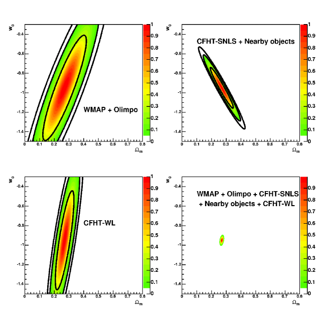
Figure 3: CL contours for mid term CMB (WMAP +Olimpo), SNIa and weak lensing data from CFHTLS and the combination of the three probes for the 8 parameter fit in the plane ($\Omega_{m},w_{0}$) (see also Tab. 4). The solid lines represent 68% (1 $\sigma$), 95% (2$\sigma$), and 99% CL contours.

The different plots in Fig. 3 show the results for individual mid term probes and for their combination. The results are for a constant $w_{0}$, plotted as a function of the matter density $\Omega_{m}$. The combined contours are drawn using the full correlation matrix on the 8 parameters for the different sets of data.

The SNLS survey combined with the nearby sample will improve the present precision on $w$ by a factor 2. The expected contours from cosmic shear have the same behaviour as the CMB but provide a slightly better constraint on $\Omega_{m}$ and a different correlation with $w$: CMB and weak lensing data have a positive ($w,\Omega_{m}$) correlation compared to SNIa data, which have a negative correlation. This explains the impressive gain when the three data sets are combined, as shown in Tab. 4. Combining WMAP with Olimpo data, helps to constrain $w$ through the correlation matrix as Olimpo expects to have more information for the large $\ell$ of the power spectrum.

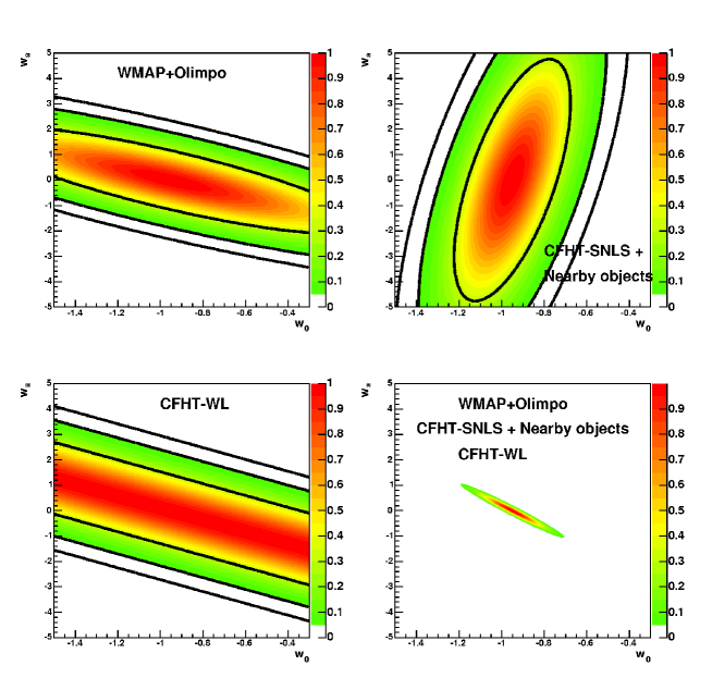
Figure 4: CL contours for mid term CMB (WMAP +Olimpo), SNIa and weak lensing data from CFHTLS and the combination of the three probes for the 9 parameter fit in the plane ($w_{0},w_{a}$) (see also Tab. 4). The solid lines represent 68% (1 $\sigma$), 95% (2$\sigma$), and 99% CL contours.

Fig. 4 gives the expected accuracy of the mid term surveys on the parameters of an evolving equation of state. The CL contours plots of $w_{a}$ versus $w_{0}$, are obtained with a 9 cosmological parameter fit. Here also, we observe a good complementarity: there is little information on the time evolution from SNIa with no prior, while the large redshift range from CMB data is adding a strong anti-correlated constraint on $w_{a}$.

A combined analysis proves far superior to analysis with only SNIa. In the favourable case, where we add more SNIa from HST survey, we expect a gain of a factor 2 on the errors, but it is not enough to lift degeneracies and the expected precision on $w_{a}$ with these data will not be sufficient to answer questions on the nature of the dark energy.

Table 4: Expected sensitivity on cosmological parameters for three scenarii: Current supernova and CMB experiments (WMAP and Riess et al.Riess04 (2004)), mid term experiments (CFHT-SNLS (supernova surveys), CFHTLS-WL (weak lensing) and CMB (WMAP+Olimpo)), long term experiments (CMB (Planck) and SNAP (supernovae and weak lensing)). For each scenario, the first column gives the $1\sigma$ error computed with the Fisher matrix techniques for the 8 free parameter configuration and the second columns gives the $1\sigma$ error for the 9 free parameter configuration.

Scenario	Today		Mid term		Long Term
${\mathbf{\Omega}_{b}}$	$0.003$	$0.004$	$0.001$	$0.002$	$0.0008$	$0.0008$
${\mathbf{\Omega}_{m}}$	$0.04$	$0.04$	$0.01$	$0.01$	$0.004$	$0.004$
${\mathbf{h}}$	$0.03$	$0.03$	$0.01$	$0.01$	$0.006$	$0.006$
${\mathbf{n}_{s}}$	$0.03$	$0.03$	$0.006$	$0.009$	$0.003$	$0.003$
${\mathbf{\tau}}$	$0.05$	$0.04$	$0.01$	$0.01$	$0.01$	$0.01$
${\mathbf{w}_{0}}$	$0.11$	$0.22$	$0.02$	$0.10$	$0.02$	$0.04$
${\mathbf{w}_{a}}$	$-$	$0.99$	$-$	$0.43$	$-$	$0.07$
${\mathbf{A}}$	$0.10$	$0.10$	$0.02$	$0.02$	$0.02$	$0.02$
${\mathbf{M}_{s0}}$	$0.03$	$0.03$	$0.01$	$0.01$	$0.01$	$0.01$

The simulated future space missions show an improved sensitivity to the time evolution of the equation of state. The accuracy on $w_{a}$ for the different combinations are summarised in Tab. 4. There is again a large improvement from the combination of the three data sets. The precision, for the long term surveys, will be sufficient to discriminate between the different models we have chosen, as shown in the left hand side plot of Fig. 5 and in Tab. 5, while it is not the case for the mid term surveys. This figure illustrates, moreover, that the errors on $w_{a}$ and $w_{0}$, and the correlation between these two variables are strongly dependent on the choice of the fiducial model.

Table 5: Expected sensitivity on cosmological parameters for the long term missions with CMB (Planck) and SNAP (supernova surveys and weak lensing) for the 9 free parameter configuration.

Model	$\mathbf{\Lambda}$CDM	SUGRA	Phantom
${\mathbf{\Omega}_{b}}$	$0.0008$	$0.0008$	$0.0007$
${\mathbf{\Omega}_{m}}$	$0.004$	$0.004$	$0.003$
${\mathbf{h}}$	$0.006$	$0.006$	$0.005$
${\mathbf{n}_{S}}$	$0.003$	$0.003$	$0.003$
${\mathbf{\tau}}$	$0.01$	$0.01$	$0.01$
${\mathbf{w}_{0}}$	$0.04$	$0.04$	$0.03$
${\mathbf{w}_{a}}$	$0.07$	$0.06$	$0.14$
${\mathbf{A}}$	$0.02$	$0.02$	$0.02$
${\mathbf{M}_{s0}}$	$0.015$	$0.014$	$0.013$

More generally, the combination of the probes with the full correlation matrix allows the extraction of the entire information available. For instance, the large correlation between $n_{S}$ and $w_{a}$ observed for the weak lensing probe combined with the precise measurement of $n_{s}$ given by the CMB, gives a better sensitivity on $w_{a}$ than the simple combination of the two $w_{a}$ values, obtained separately for the CMB and weak lensing. Such an effect occurs for several other pairs of cosmological parameters considered in this study. The plot, in the right hand side of Fig 5, is an illustration of this effect. It shows the combination of the 3 probes in the ($w_{0},w_{a}$) plane. The $1\sigma$ contour for the combined three probes, is more constraining than the 2-D combination in the ($w_{0},w_{a}$) plane of the three probes.

Finally, in the long term scenario, the weak lensing probe provides a sensitivity on the measurement of $(w_{0},w_{a})$ comparable with those of the combined SN and CMB probes, whereas in the mid term scenario the information brought by weak lensing was marginal. This large improvement observed in the information provided by the weak lensing, can be explained by the larger survey size and the deeper volume probed by SNAP/JDEM, compared to the ground CFHTLS WL survey. We thus conclude that adding weak lensing information will be an efficient way to help distinguishing between dark energy models. If systematic effects are well controlled, the future dedicated space missions may achieve a sensitivity of order 0.1 on $w_{a}$.

The SNAP/JDEM space mission is designed, in principle, to control its observational systematic effects for SNIa to the $\%$ level, which is probably impossible to reach for future ground experiments. In this study, we assign an irreducible systematic error on SNIa magnitudes of 0.02 and systematic effects have been neglected for CMB and weak lensing. This can have serious impacts on the final sensitivity, in particular, on the relative importance of each probe.

Other probes, whose combined effects we have not presented in this paper, but intend to do in forthcoming studies, remain therefore most useful. For example, the recent evidence for baryonic oscillations (Eisenstein et al. 2005) is a proof that new probes can be found. The present constraints that these results provide, do not improve the combined analysis we present here. However, getting similar results from different probes greatly contributes to the credibility of a result, in particular, when the systematical effects can be quite different, as is the case for the different probes we consider. Finally, the joint analysis of cluster data observed simultaneously with WL, SZ effect and X-rays, will allow the reduction of the intrinsic systematics of the WL probe.

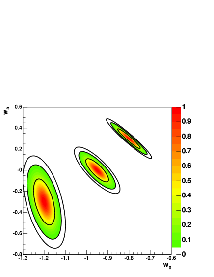
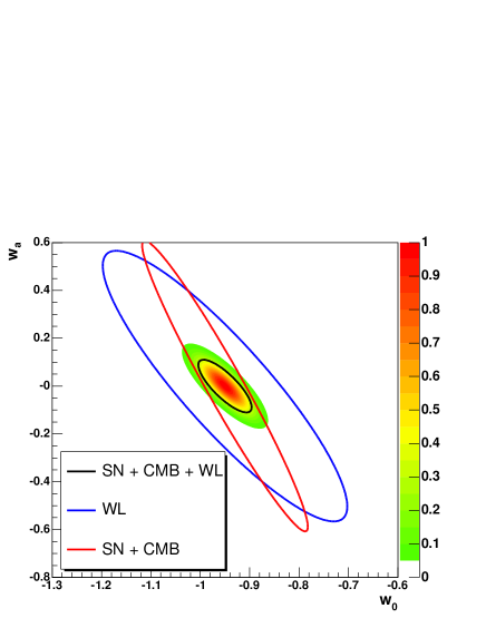
Figure 5: CL contours for future space data from SNAP (SNIa and WL) and Planck (CMB) for a 9 parameter fit in the plane ($w_{0},w_{a}$). The left hand side figure shows the combination of SNAP (SNIa+WL) and CMB for three different models ($\Lambda$CDM, SUGRA and Phantom). The solid lines represent 68% (1 $\sigma$), 95% (2$\sigma$), and 99% CL contours. The right hand side figure shows the CL for the combined three ”long term” probes. The solid lines are the 1$\sigma$ contours for different combinations: WL alone, combined SNIa and CMB, and the three combined probes.

5 Conclusions

In this paper, we have presented a statistical method based on a frequentist approach to combine different cosmological probes. We have taken into account the full correlations of parameters without any priors, and without the use of Markov chains.

Using current SNIa and WMAP data, we fit a parametrization of an evolving equation of state and find results in good agreement with other studies in the literature. We confirm that data prefer a value of $w$ less than -1 but are still in good agreement with the $\Lambda CDM$ model. We emphasise the impact of the implementation of the dark energy perturbations. This can explain the discrepancies in the central values found by various authors. We have performed a complete statistical treatment, evaluated the errors for existing data and validated that the Fisher matrix technique is a reliable approach as long as the parameters $(w_{0},w_{a})$ are in the ‘physical’ region imposed by CMB boundary condition: $w(z\to\infty)<0$.

We have then used the Fisher approximation to calculate the expected errors for current surveys on the ground (e.g., CFHTLS) combined with CMB data, and compared them with the expected improvements from future space experiments. We confirm that the complete combination of the three probes, including weak lensing data, is very powerful for the extraction of a constant $w$. However, a second generation of experiments like the Planck and SNAP/JDEM space missions is required, to access the variation of the equation of state with redshift, at the 0.1 precision level. This level of precision needs to be confirmed by further studies of systematical effects, especially for weak lensing.

- (1) Aldering G. et al., SNAP Collaboration, 2004, astro-ph/0405232
- (2) Bacon, D.J., Refregier, A., & Ellis, R., 2000, MNRAS 318, 625
- (3) Bacon, D.J., Refregier, A., Clowe, D., Ellis, R. , 2001, MNRAS 325, 1065
- (4) Bardeen, J.M., Bond, J.R., Kaiser, N., Szalay, A.S., 1986, Astrophys.J. 304, 15
- (5) Bartelmann, M., & Schneider, P., 2001, Phys. Rep. 340, 291
- (6) Benabed K. & Van Waerbeke L., 2004, Phys. Rev. D70, 123515
- (7) Bennett C.et al., (WMAP Collaboration), 2003, Astrophys. J. Suppl. 148, 1
- (8) Bunn E. & White S., 1997, Astrop. J. 480, 6
- (9) Bridle S.L.et al., 2003, Science 299, 1532
- (10) Caldwell, R.R., 2002, Phys. Lett. B. 545, 23
- (11) CFHTLS: see e.g. http://cfht.hawaii.edu, http://cfht.hawai.edu/Science/CFHTLS-OLD/history2001.html
- (12) Caldwell R.R. and Doran M., 2005, astro-ph/0501104
- (13) Carlin B.P. and Louis T.A., Bayes and Empirical Bayes Methods for Data Analysis, 1996, (Chapman and Hall, London)
- (14) Carroll S.M. et al., 2005, Phys.Rev. D71, 063513
- (15) Chevallier M.& Polarski D., 2001, Int.J.Mod.Phys. D10, 213
- (16) Christensen N. and Meyer R., 1998, Phys. Rev. D58, 082001
- (17) Cooray, A., & Hu, W., 2001, Astrophys. J. 554, 56
- (18) Corasaniti P. et al., 2004, Phys.Rev. D70, 083006
- (19) Doran M., 2003, astro-ph/0302138
- (20) Eisenstein et al., 2005, astro-ph/0501171
- (21) Fisher, R.A. 1935, J. Roy. Stat. Soc. 98, 39
- (22) Feldman G.J., Cousins R.D., 1998, Phys. Rev. D57, 3873
- (23) Gerke B. F. & Efstathiou G., 2002, MNRAS 335, 33
- (24) Gilks W.R., Richardson S., Spiegelhalter D. J., 1996, Markov Chain Monte Carlo in Practice (Chapman and Hall, London)
- (25) Hawkins E. et al., 2003, MNRAS 347, 78
- (26) Heymans C. et al., 2005, astro-ph/0506112
- (27) Hoekstra, H., Yee, H., & Gladders, M., 2002, New Astron. Rev.46, 767
- (28) Hu, W., & Tegmark, M., 1999, Astrophys.J. 514, L65
- (29) Hu, W., 1999, Astrophys. J. 522, L21
- (30) Hu, W., 2002, Phys. Rev. D65 023003
- (31) Hu, W., 2004, preprint astro-ph/0407158
- (32) Huterer, D., 2001, Phys. Rev. D65, 063001
- (33) Huterer, D. and Turner, M.S., 2001, Phys. Rev. D64 123527
- (34) Ishak M., 2005, astro-ph/0501594.
- (35) James F., 1978, CERN Program Library Long Writeup, D506.
- (36) Kaiser, N., 1998, Astrophys.J. 498, 26.
- (37) Kim A.G.et al., 2004, Mon. Not. R. Astron Soc. 347, 909
- (38) Knop R.A.et al., 2003, Astrophys. J. 598, 102
- (39) Knox L., 1995, Phys. Rev. D52, 4307
- (40) Lewis A. & Bridle S., 2002, Phys. Rev D66, 103511
- (41) Linder E.V., 2003, Phys. Rev. Lett. 90, 091301
- (42) Linder E.V. & Jenkins A., 2003, MNRAS 346, 573
- (43) Linder E.V. and Huterer D., 2005, astro-ph/0505330
- (44) Lue A., Scoccimaro R. and Starkman G., 2004, Phys. Rev. D69, 044005
- (45) Ma, C.-P., Caldwell, R.R., Bode, P., & Wang, L., 1999, Astrophys.J. 521, L1
- (46) Maor I.et al., 2001, Phys. Rev. Lett. 86, 6
- (47) Maor I. et al., 2002, Phys. Rev. D65, 123003
- (48) Masi S. et al., Olimpo Collaboration, 2003, Mem. S.A.It. Vol 74, 96
- (49) Massey R. et al., 2004, Astron. J. 127 3089
- (50) Mellier, Y. et al., 2002, SPIE Conference 4847 Astronomical Telescopes and Instrumentation, Kona, August 2002, preprint astro-ph/0210091
- (51) Neyman J., Phil. Trans. Royal Soc. London, Series A, 236, 333-80.
- (52) Peacock, J.A., & Dodds, 1996, MNRAS 280 L19
- (53) Peacock, J.A., 1997, MNRAS 284 885
- (54) Peebles P.J.E. & Ratra R., 1988, Astrophys. J. Lett. 325 L17
- (55) Rapetti D., Allen S., Weller J., 2004, astro-ph/0409574, accepted, MNRAS
- (56) Refregier A., 2003, ARAA 41, 645
- (57) Refregier A. et al., 2004, Astron.J. 127, 3102
- (58) Rhodes J.et al., 2004, Astrophys.J. 605 29
- (59) Riess A.G. et al., 2004, Astrophys. J. 607, 665
- (60) Seljak U. & Zaldarriaga M., 1996, Astrophys. J. 469, 437
- (61) Seljak U.et al., astro-ph/0407372
- (62) Spergel D.N., 2003, Astrophys.J.Suppl. 148, 175
- (63) SNLS http://cfht.hawaii.edu/Science/CFHTLS-OLD/history2001.html, cf e.g. http://cfht.hawaii.eduSNLS
- (64) Sugiyama N., 1995, Astrophys.J.Suppl. 100, 281
- (65) Sunyaev R.A. and Zeldovich Ya.B., 1980, Ann. Rev. Astron. Astrophys. 18, 537
- (66) Tauber J.A. et al., Planck Collaboration, 2004, Advances in Space Research, 34, 491
- (67) Tilquin A.,2003,
- (68) Tegmark M. et al., 2004, Phys. Rev. D69, 103501
- (69) Upadhye A.et al., astro-ph/0411803
- (70) Virey J.-M. et al., 2004a, Phys. Rev. D70, 043514
- (71) Virey J.-M. et al., 2004b, Phys. Rev. D70, 121301
- (72) Wang Y. & Tegmark M., 2004, Phys. Rev. Lett. 92, 241302
- (73) Weller J. & Albrecht A., 2002, Phys. Rev. D65, 103512
- (74) Weller J. & Lewis A.M , 2003, MNRAS 346, 987
- (75) Wetterich C., 1988, Nucl. Phys. B302, 668
- (76) Wood-Vasey W.M.et al., Nearby Supernova Factory, 2004, New Astron.Rev. 48, 637
- (77) Xia J.-Q., Feng B. & Zhang X.-M., 2004, astro-ph/0411501
- (78) Zech, G., 2002, Eur.Phys.J.direct C4, 12