The Dipole Anisotropy of the 2 Micron All-Sky Redshift Survey

Abstract

We estimate the acceleration on the Local Group (LG) from the Two Micron All Sky Redshift Survey (2MRS). The sample used includes about 23,200 galaxies with extinction corrected magnitudes brighter than $K_{\rm s}=11.25$ and it allows us to calculate the flux weighted dipole. The near-infrared flux weighted dipoles are very robust because they closely approximate a mass weighted dipole, bypassing the effects of redshift distortions and require no preferred reference frame. This is combined with the redshift information to determine the change in dipole with distance. The misalignment angle between the LG and the CMB dipole drops to 12${}^{\circ}\pm$7^∘ at around 50 $h^{-1}{\rm Mpc}$, but then increases at larger distances, reaching 21${}^{\circ}\pm$8^∘ at around 130 $h^{-1}{\rm Mpc}$. Exclusion of the galaxies Maffei 1, Maffei 2, Dwingeloo 1, IC342 and M87 brings the resultant flux dipole to 14${}^{\circ}\pm$7^∘ away from the CMB velocity dipole In both cases, the dipole seemingly converges by 60 $h^{-1}{\rm Mpc}$. Assuming convergence, the comparison of the 2MRS flux dipole and the CMB dipole provides a value for the combination of the mass density and luminosity bias parameters ${\Omega_{\rm m}}^{0.6}/b_{\rm L}=0.40\pm 0.09$.

1 Introduction

The most popular mechanism for the formation of large-scale structure and motions in the Universe is the gravitational growth of primordial density perturbations. According to this paradigm, if the density perturbations are small enough to be approximated by a linear theory, then the peculiar acceleration vector ${\bf g}({\bf r})$ induced by the matter distribution around position ${\bf r}$ is related to the mass by

$${\bf g}({\bf r})=G\bar{\rho}\int\limits_{\bf r}^{\infty}d^{3}{\bf r}^{\prime}\delta_{m}({{\bf r}^{\prime}})\frac{{\bf r}^{\prime}-{\bf r}}{|{\bf r}^{\prime}-{\bf r}|^{3}}$$ (1)

where $\bar{\rho}$ is the mean matter density and $\delta_{m}({\bf r})$ = $(\rho_{m}({\bf r})-\bar{\rho})/\bar{\rho}$ is the density contrast of the mass perturbations. In linear theory, the peculiar velocity field, ${\bf v}({\bf r})$, is proportional to the peculiar acceleration:

$${\bf v}({\bf r})=\frac{H_{0}f(\Omega_{\rm m})}{4\pi G\bar{\rho}}{\bf g}({\bf r})=\frac{2f(\Omega_{\rm m})}{3H_{0}\Omega_{\rm m}}{\bf g}({\bf r}),$$ (2)

where $H_{0}$ = 100 $h$ ${\rm km}{\rm s}^{-1}{\rm Mpc}^{-1}$ is the Hubble constant and $f(\Omega_{\rm m})\approx\Omega_{\rm m}^{0.6}$ is the logarithmic derivative of the amplitude of the growing mode of the perturbations in mass with respect to the scale factor (Peebles 1980). The factor $f(\Omega_{\rm m})$ is only weakly dependent on the cosmological constant (Lahav et al. 1991).

During the past twenty five years, particular attention has been paid to the study of the gravitational acceleration and the peculiar velocity vectors of the Local Group (LG) of galaxies. It is now widely accepted that the cosmic microwave background (CMB) dipole is a Doppler effect arising from the motion of the Sun (but see e.g. Gunn 1988 and Paczyński & Piran 1990 who argue that the CMB dipole is of primordial origin). In this case, the dipole anisotropy of the CMB is a direct and accurate measurement of the LG peculiar velocity (c.f. Conklin 1969 and Henry 1971). The LG acceleration can also be estimated using surveys of the galaxies tracing the density inhomogeneities responsible for the acceleration. By comparing the CMB velocity vector with the acceleration vector obtained from the galaxy surveys, it is possible to investigate the cause of the LG motion and its cosmological implications. This technique was first applied by Yahil, Sandage & Tammann (1980) using the Revised Shapley-Ames catalogue and later by Davis & Huchra (1982) using the CfA catalogue. Both catalogues were two-dimensional and the analyses were done using galaxy fluxes. Since both the gravity and the flux are inversely proportional to the square of the distance, the dipole vector can be calculated by summing the flux vectors and assuming an average value for the mass-to-light ratio. Lahav (1987) applied the same method to calculate the dipole anisotropy using maps based on three galaxy catalogues, UGC, ESO, MCG. The most recent application of the galaxy flux dipole analysis was carried out by Maller et al. (2003), using the two-dimensional Two Micron All-Sky Survey (2MASS) extended source catalogue (XSC), with a limiting magnitude of $K_{\rm s}=13.57$. They found that the LG dipole direction is 16^∘ away that of the CMB.

Our ability to study the LG motion was greatly advanced by the whole-sky galaxy samples derived from $IRAS$ Galaxy Catalogues. Yahil, Walker & Rowan-Robinson (1986), Meiksin & Davis (1986), Harmon, Lahav & Meurs (1987), Villumsen & Strauss (1987) and Lahav, Rowan-Robinson & Lynden-Bell (1988) used the two-dimensional $IRAS$ data to obtain the LG dipole. The dipole vectors derived by these authors are in agreement with each other and the CMB dipole vector to within 10^∘-30^∘ degrees. The inclusion of galaxy redshifts in the dipole analyses allowed the estimation of the distance at which most of the peculiar velocity of the LG is generated (the convergence depth). However, the estimates of the convergence depth from various data sets have not agreed. Strauss et al. (1992, $IRAS$ sample), Webster, Lahav & Fisher (1997, $IRAS$ sample), Lynden-Bell, Lahav & Burstein (1989, optical sample) and da Costa et al. (2000, a sample of early-type galaxies) suggested that the LG acceleration is mostly due to galaxies $\lesssim 50h^{-1}{\rm Mpc}$, while other authors such as Scaramella, Vettolani & Zamorani (1994, Abell/ACO cluster sample), Branchini & Plionis (1996, Abell/ACO cluster sample), Kocevski et al. (2004) and Kocevski & Ebeling (2005, both using samples of X-ray clusters) claimed that there is significant contribution to the dipole from depths of up to $\approx$200 $h^{-1}{\rm Mpc}$.

Dipole analyses are often used to estimate the combination of matter density and biasing parameters ${\Omega_{\rm m}}$ and $b$. In theory, one can equate the velocity inferred from the CMB measurements with the value derived from a galaxy survey and obtain a value for $\beta$. In practice, however, the galaxy surveys do not measure the true total velocity due their finite depth (e.g. Lahav, Kaiser & Hoffman 1990 and Juszkiewicz, Vittorio & Wyse 1990). The true ${\bf v}_{LG}$, as obtained from the CMB dipole, arises from structure on all scales including structures further away than the distance a galaxy survey can accurately measure. Furthermore, the magnitude/flux/diameter limit of the survey and any completeness variations over the sky introduce selection effects and biases to the calculations. These effects amplify the errors at large distances (for redshift surveys) and faint magnitudes (for two dimensional surveys) where the sampling of the galaxy distribution becomes more sparse. This, combined with the fact that we sample discretely from an underlying continuous mass distribution leads to an increase in shot noise error. There may also be a significant contribution to the dipole from galaxies behind the Galactic Plane (the zone of avoidance). The analysis of the convergence of the dipole is further complicated by the redshift distortions on small and large scales which introduce systematic errors to the derived dipole (the rocket effect, Kaiser 1987). The following sections discuss these effects in the context of two different models of biasing.

In this paper, we use the Two Micron All-Sky Redshift Survey (2MRS, Huchra et al. 2005) to study the LG dipole. The inclusion of the redshift data allows the calculation of the selection effects of the survey as a function of distance and enables the study of convergence and thus improves the analysis of Maller et al. (2003). The paper is structured as follows: The Two Micron Redshift Survey is described in Section 2. Section 3 discusses the method used in the analysis including the different weighting schemes, the rocket effect and the choice of reference frames. The results are presented in Section 4. The final section includes some concluding remarks and plans for future work.

2 The Two Micron All-Sky Redshift Survey

The Two Micron All-Sky Redshift Survey (2MRS) is the densest all-sky redshift survey to date. The galaxies in the northern celestial hemisphere are being observed mainly by the FLWO 1.5-m telescope and at low latitudes by the CTIO. In the southern hemisphere, most galaxies are observed as a part of the six degree field galaxy survey (6dFGS, Jones et al. 2004) conducted by the Anglo Australian Observatory. The first phase of the 2MRS is now completed. In this phase we obtained redshifts for approximately 23,000 2MASS galaxies from a total sample of about 24,800 galaxies with extinction corrected magnitudes (Schlegel, Finkbeiner & Davis 1998) brighter than $K_{\rm s}=11.25$. This magnitude limit corresponds to a median redshift of $z\approx 0.02$ ($\approx 60h^{-1}$ Mpc). The majority of the 1600 galaxies that remain without redshifts are at very low galactic latitudes or obscured/confused by the dust and the high stellar density towards the Galactic Centre. Figure 1 shows all the objects in the 2MRS in Galactic Aitoff Projection. Galaxies with ${\rm z}\leq 0.01$ are plotted in red, $0.01<{\rm z}\leq 0.025$ are plotted in blue, $0.025<{\rm z}<0.05$ are plotted in green and ${\rm z}\geq 0.05$ are plotted in magenta. Galaxies without measured redshifts are plotted in black. The 2MRS can be compared with the deeper 2MASS galaxy catalogue (K$<$14th mag) shown in Jarrett (2004, Figure 1).

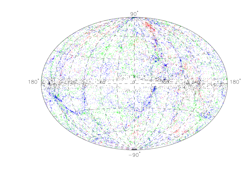
Figure 1: All Objects in the 2MASS Redshift Catalogue in Galactic Aitoff Projection. Galaxies with ${\rm z}\leq 0.01$ are plotted in red, $0.01<{\rm z}\leq 0.025$ are plotted in blue, $0.025<{\rm z}<0.05$ are plotted in green and ${\rm z}\geq 0.05$ are plotted in magenta. Galaxies without measured redshifts are plotted in black. The masked region is outlined by dashed lines.

2.1 Survey Completeness

The 2MASS has great photometric uniformity and an unprecedented integral sky coverage. The photometric uniformity is better than $4\%$ over the sky including the celestial poles (e.g. Jarrett et al. 2000$a$, 2003). The uniform completeness of the galaxy sample is limited by the presence of the foreground stars. For a typical high latitude sky less than $2\%$ of the area is masked by stars. These missing regions are accounted for using a coverage map, defined as the fraction of the area of an 8′$\times$8′pixel that is not obscured by stars brighter than 10th mag. Galaxies are then weighted by the inverse of the completeness although the analysis is almost unaffected by this process as the completeness ratio is very close to one for most parts of the sky.

The stellar contamination of the catalogue is low and is reduced further by manually inspecting the objects below a redshift of $cz=200$${\rm\thinspace km}{\rm\thinspace s}^{-1}$. The foreground stellar confusion is highest at low Galactic latitudes, resulting in decreasing overall completeness of the 2MASS catalogue (e.g. Jarrett et al. 2000$b$) and consequently the 2MRS sample. Stellar confusion also produces colour bias in the 2MASS galaxy photometry (Cambresy, Jarrett & Beichman 2005) but this bias should not be significant for the 2MRS because of its relatively bright magnitude limit.

In order to account for incompleteness at low Galactic latitudes we fill the Zone of Avoidance (the plane where $|b|<5^{\circ}$ and $|b|<10^{\circ}$ in the region $|l|<30^{\circ}$) with galaxies. We keep the galaxies with observed redshifts and apply two different methods to compensate for the unobserved (masked) sky:

• Method 1: The masked region is filled with galaxies whose fluxes and redshifts are chosen randomly from the whole data set. These galaxies are placed at random locations within the masked area. The masked region has the same average density of galaxies as the rest of the sky.

• Method 2: The masked region is filled following Yahil et al. (1991). The area is divided into 36 bins of $10^{\circ}$ in longitude. In each angular bin, the distance is divided into bins of 1000 ${\rm\thinspace km}{\rm\thinspace s}^{-1}$. The galaxies in each longitude/distance bin are then sampled from the corresponding longitude/distance bins in the adjacent strips $-|b_{masked}|-10^{\circ}<b<|b_{masked}|+10^{\circ}$ (where $|b_{masked}|=5^{\circ}$ or $|b_{masked}|=10^{\circ}$). These galaxies are then placed in random latitudes within the mask region. This procedure gives similar results to the more elaborate method of Wiener reconstruction across the zone of avoidance (Lahav et al. 1994). The number of galaxies in each masked bin is set to a random Poisson deviate whose mean equals to the mean number of galaxies in the adjacent unmasked strips. This procedure is carried out to mimic the shot noise effects.

In reality, the shape of the Zone of Avoidance is not as symmetric as defined in this paper with Galactic Bulge centred at $l\approx+5^{\circ}$ and with latitude offsets (see Kraan-Korteweg 2005). However, since we keep the galaxies in the masked regions, our dipole determinations should not be greatly influenced by assuming a symmetric mask. We test this by changing the centre of the Galactic bulge. We confirm that our results are not affected. Figure 2 shows the 2MRS galaxies used in the analyses in a Galactic Aitoff projection. The galaxies in masked regions are generated using the first (top plot) and the second method (bottom plot).

$\begin{array}[]{c}\psfig{angle=0,width=390.25534pt,height=213.39566pt,clip={}}\\ \psfig{angle=0,width=390.25534pt,height=213.39566pt,clip={}}\\ \end{array}$

Figure 2: Top: Objects in the 2MASS Redshift Catalogue used in the analysis in a Galactic Aitoff Projection, including the random galaxies generated by using the first technique. Galaxies with ${\rm z}\leq 0.01$ are plotted in red, $0.01<{\rm z}\leq 0.025$ are plotted in blue, $0.025<{\rm z}<0.05$ are plotted in green and ${\rm z}\geq 0.05$ are plotted in magenta.Bottom: Same as the top plot but now including the random galaxies generated in using the second technique. The regions inside the dashed lines in the plots are masked out and replaced with the random galaxies shown in the plots. There are 21510 galaxies in each plot.

2.2 Magnitude and Flux Conversions

The 2MRS uses the 2MASS magnitude $K_{20}$, which is defined as the magnitude inside the circular isophote corresponding to a surface brightness of $\mu_{K_{s}}=20{\rm mag}$ arcsec^-2 (e.g. Jarrett et al. 2000$a$). The isophotal magnitudes underestimate the total luminosity by $10\%$ for the early-type and $20\%$ for the late-type galaxies (Jarrett et al. 2003). Following Kochanek et al. (2001, Appendix), the offset of $\Delta=-0.20\pm 0.04$ is added to the $K_{20}$ magnitudes. The galaxy magnitudes are corrected for Galactic extinction using the dust maps of Schlegel, Finkbeiner & Davis (1998) and an extinction correction coefficient of $R_{K}=0.35$ (Cardelli, Clayton & Mathis 1989). As expected, the extinction corrections are small for the 2MRS sample. The $K_{\rm s}$ band $k$-correction is derived by Kochanek et al. (2001) based on the stellar population models of Worthey (1994). The k-correction of $k(z)=-6.0\log(1+z)$, is independent of galaxy type and valid for $z\lesssim 0.25$.

The fluxes $S$ are computed from the apparent magnitudes using

$$S=S(0\,{\rm mag})10^{-0.4(K_{20}+ZPO)}$$ (3)

where the zero point offset is $ZPO=0.017\pm 0.005$ and $S(0{\rm mag})=1.122\times 10^{-14}\pm 1.891\times 10^{-16}{\rm Wcm}^{-2}$ for the $K_{\rm s}$ band (Cohen, Wheaton & Megeath 2003).

2.3 The Redshift Distribution and the Selection Function

The redshift distribution of the 2MRS is shown in Figure 3. The $IRAS$ PSCz survey redshift distribution (Saunders et al. 2000) is also plotted for comparison. The 2MRS samples the galaxy distribution better than the PSCz survey out to $cz=15000$${\rm\thinspace km}{\rm\thinspace s}^{-1}$. The selection function of the survey (i.e. the probability of detecting a galaxy as a function of distance) is modeled using a parametrised fit to the redshift distribution:

$$dN(z)=Az^{\gamma}\exp\left[-\left(\frac{z}{z_{c}}\right)^{\alpha}\right]dz\;,$$ (4)

with best-fit parameters of $A=116000\pm 4000$, $\alpha=2.108\pm 0.003$, $\gamma=1.125\pm 0.025$ and $z_{c}=0.025\pm 0.001$. This best-fit is also shown in Figure 3 (solid line). The overall selection function $\phi(r)$ is the redshift distribution divided by the volume element

$$\phi(r)=\frac{1}{\Omega_{s}r^{2}}\left(\frac{dN}{dz}\right)_{r}\left(\frac{dz}{dr}\right)_{r}\;$$ (5)

where $\Omega_{s}(\approx 4\pi$ steradians) is the solid angle of the survey and $r$ is the comoving distance.

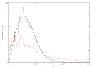
Figure 3: Redshift histogram for 2MRS galaxies and a least squares fit (Equation 4) to the data (black). For comparison, also plotted is a redshift histogram for PSCz galaxies (Saunders et al. 2000) (red).

2.4 Taking out the Local Group Galaxies

Galaxies that are members of the Local Group need to be removed from the 2MRS catalogue to maintain the internal consistency of the analysis. We used the Local Group member list of thirty five galaxies (including Milky Way) given in Courteau and Van den Bergh (1999) to identify and remove eight LG members (IC 10, NGC 147, NGC 185, NGC 205, NGC 6822, M31, M32, M33) from our analysis. In Section 4, we will calculate the acceleration on to the Milky Way due to these LG members.

2.5 Assigning distances to nearby Galaxies

In order to reduce the distance conversion errors, we cross-identified 35 galaxies which have HST Key Project distances (see Freedman et al. 2001 and the references therein) and 110 galaxies which have distance measurements compiled from several sources (see Karachentsev et al. 2004 and the references therein). We assign these galaxies measured distances instead of converting them from redshifts. In addition, we identify nine blue-shifted galaxies in the 2MRS which are members of the Virgo cluster. We assign these galaxies the distance to the centre of Virgo ($\approx 15.4$ Mpc, Freedman et al. 2001). Finally, there are four remaining blue-shifted galaxies without known distance measurements which are assigned to 1.18 $h^{-1}$ Mpc . Thus by assigning distances to galaxies, we do not need to exclude any non-LG galaxy from the analysis.

3 The Methods and Weighting Schemes

In order to compare the CMB and the LG dipoles, it is necessary to postulate a relation between the galaxy distribution and the underlying mass distribution. In this paper, we will use both a number weighted and a flux weighted prescription. Although quite similar in formulation, these schemes are based on very different models for galaxy formation. The number weighted prescription assumes that the mass distribution in the Universe is a continuous density field and that the galaxies sample this field in a Poisson way. On the other hand, the flux weighted model is based on the assumption that the mass in the Universe is entirely locked to the mass of the halos of the luminous galaxies.

3.1 Number Weighted Dipole

It is commonly assumed that the galaxy and the mass distributions in the Universe are directly proportional to each other and are related by a proportionality constant, the linear bias parameter $b$: $\delta n/n\equiv\delta_{g}=b\delta_{m}$. In this case, Equation 2 for the LG can be rewritten as

$${\bf v}_{LG}=\frac{H_{0}\beta}{4\pi}\int_{{\bf r}}^{\infty}d^{3}{\bf r}^{\prime}\delta_{g}({{\bf r}^{\prime}})\frac{{\bf r}^{\prime}-{\bf r}}{|{\bf r}^{\prime}-{\bf r}|^{3}}$$ (6)

where $\beta\equiv{\Omega_{\rm m}}^{0.6}/b$.

For the number weighted model, incomplete sampling due to the magnitude limit is described by the selection function, $\phi(r)$ given in Section 2.3. Each galaxy $i$ is assigned a weight:

$$w_{i}=\frac{1}{\phi(r_{i})C_{i}}$$ (7)

where $\phi(r_{i})$ and $C_{i}$ are the values of the radial selection function and the completeness ($0\leq C_{i}\leq 1$) for each galaxy, respectively. The observed velocity of the Local Group with respect to the CMB is given by

$${\bf v}({\bf r})=\frac{H_{0}\beta}{4\pi\bar{n}}\sum\limits_{i}^{N}\,\frac{w_{i}\hat{{\bf r}}_{i}}{r_{i}^{2}}$$ (8)

where $\bar{n}$ is the mean galaxy density of the survey and $\hat{{\bf r}}_{i}$ is the unit vector of the galaxy’s position. The sum in the equation is over all galaxies in the sample that lie in the distance range $r_{min}<r_{i}<r_{max}$. Calculated this way, the velocity vector does not depend on the Hubble constant ($h$ cancels out).

If the galaxies are assumed to have been drawn by a Poisson point process from an underlying density field, then it is straightforward to calculate the shot noise errors. The shot noise is estimated as the $rms$ of the cumulative variance, $\sigma_{sn}^{2}$ given by

$$\sigma_{sn}^{2}=\left(\frac{H_{0}\beta}{4\pi\bar{n}}\right)^{2}\sum\limits_{i}^{N}\,\left(\frac{\hat{{\bf r}}_{i}}{r_{i}^{2}\phi(r_{i})C_{i}}\right)^{2}\;.$$ (9)

The shot noise error per dipole component is $\sigma_{1D}=\sigma_{sn}/\sqrt{3}$.

3.2 Flux Weighted Dipole

For this model, each galaxy is a ‘beacon’ which represents the underlying mass. This is characterised by the mass-to-light ratio $\Upsilon={\rm M}/{\rm L}$. $\Upsilon$ is probably not constant and varies with galaxy morphology (e.g. Lanzoni et al. 2004) but mass-to-light ratios of galaxies vary less in the near-infrared than in the optical (e.g. Cowie et al. 1994; Bell & de Jong 2001). In the context of dipole estimation, this model of galaxy formation implies that the Newtonian gravitational acceleration vector for a volume limited sample is

$${\bf g}({\bf r}) = {\rm G}\sum\limits_{i}\,M_{i}\frac{\hat{{\bf r}}_{i}}{r_{i}^{2}}\backsimeq{\rm G}\left\langle\frac{M}{L}\right\rangle\sum\limits_{i}\,L_{i}\frac{\hat{{\bf r}}_{i}}{r_{i}^{2}}$$ (10)

$$= 4\pi{\rm G}\left\langle\frac{M}{L}\right\rangle\sum\limits_{i}\,{\rm S}_{i}\hat{{\bf r}}_{i},\vspace{2mm}$$

where the sum is over all galaxies in the Universe, $\left\langle M/L\right\rangle$ is the average mass-to-light ratio and ${\rm S}_{i}=L_{i}/4\pi r^{2}$ is the flux of galaxy $i$. The peculiar velocity vector is derived by substituting Equation 10 into the second line of Equation 2. For a flux limited catalogue the observed LG velocity is

$${\bf v}({\bf r})=\frac{8\pi{\rm G}f(\Omega_{\rm m})}{3H_{0}\Omega_{\rm m}b_{\rm L}}\left\langle\frac{M}{L}\right\rangle\sum\limits_{i}\,w_{L_{i}}{\rm S}_{i}\hat{{\bf r}}_{i}$$ (11)

where $b_{\rm L}$ is the luminosity bias factor introduced to account for the dark matter haloes not fully represented by 2MRS galaxies and $w_{L_{i}}$ is the weight assigned to galaxy $i$ derived in the next section. The mass-to-light ratio, assumed as constant, is given by

$$\left\langle\frac{M}{L}\right\rangle=\frac{\rho_{\rm m}}{\rho_{\rm L}}=\frac{3H_{0}^{2}\Omega_{\rm m}}{8\pi G\rho_{\rm L}}$$ (12)

where $\rho_{\rm L}$ is the luminosity density so Equation 11 is rewritten as:

$${\bf v}({\bf r})=\frac{H_{0}f(\Omega_{\rm m})}{\rho_{\rm L}b_{\rm L}}\sum\limits_{i}^{N}\,w_{L_{i}}{\rm S}_{i}\hat{{\bf r}}_{i}.$$ (13)

The flux weighting method (originally proposed by Gott) has been applied extensively to two-dimensional galaxy catalogues (e.g. Yahil, Walker & Rowan-Robinson 1986, Villumsen & Strauss 1987, Lahav, Rowan-Robinson & Lynden-Bell 1988) and most recently to 2MASS XSC (Maller et al. 2003). Since these surveys lack radial information, the dipoles were calculated by either assuming $w_{L_{i}}=1$ (e.g. Maller et al. 2003) or by using a luminosity function based on a redshift survey in a section of the two-dimensional catalogue (e.g. Lahav, Rowan-Robinson & Lynden-Bell 1988). In either case, it was not possible to determine the convergence of the dipole as a function of redshift. The three-dimensional $IRAS$ dipoles (Strauss et al. 1990, Webster, Lahav & Fisher 1997, Schmoldt et al. 1999 and Rowan-Robinson et al. 2000) were derived using the number weighted scheme because the $IRAS$ catalogues are biased towards star forming galaxies with widely varying mass-to-light ratios resulting in a very broad luminosity function making it difficult to estimate the distance. The 2MRS is mainly sensitive to total stellar mass rather than instantaneous star formation rates (e.g. Cole et al. 2001) and consequently the 2MRS mass-to-light ratios do not have as much scatter. Thus, for the first time, the 2MRS enables the determination the convergence of the flux dipole as a function of distance. There are many advantages to using the flux weighted model for the dipole calculation and these will be discussed in the coming sections.

For the flux weighted case, the weighting function is derived as follows: Let $\rho_{\rm L}({\rm L}\geq 0)$ be the luminosity density in the volume element $\delta V$ of a volume limited catalogue. In this case the dipole velocity is simply

$${\bf v}({\bf r})=\frac{H_{0}f(\Omega_{\rm m})}{\rho_{\rm L}b_{\rm L}}\sum\limits_{i}^{N}\,\frac{\delta V_{i}\rho_{\rm L}({\rm L_{i}}\geq 0)\hat{{\bf r}}_{i}}{r_{i}^{2}}.$$ (14)

In practice, however, we have a flux limited catalogue with $S\geq S_{\rm lim}$ so only galaxies with luminosity $L\geq L_{\rm lim}=4\pi r^{2}S_{\rm lim}$ are included in the survey. Thus the total luminosity in the infinitesimal volume $\delta V$ is

$$\delta V\rho_{\rm L}({\rm L}\geq 0)=L_{\rm obs}+\delta V\rho_{\rm L}({\rm L}<{\rm L}_{\rm lim})$$ (15)

where $L_{\rm obs}=\delta V\rho_{\rm L}({\rm L}\geq{\rm L}_{\rm lim})$ is the observed luminosity and $\delta V\rho_{\rm L}({\rm L}<{\rm L}_{\rm lim})$ is the luminosity that was not observed due to the flux limit of the survey. Substituting

$$\delta V=\frac{L_{\rm obs}}{\rho_{\rm L}({\rm L}\geq{\rm L}_{\rm lim})}$$ (16)

into Equation 15 yields

$$\delta V\rho_{\rm L}({\rm L}\geq 0) = L_{\rm obs}\Bigg{[}1+\frac{\rho_{\rm L}({\rm L}<{\rm L}_{\rm lim})}{\rho_{\rm L}({\rm L}\geq{\rm L}_{\rm lim})}\Bigg{]}$$ (17)

$$= L_{\rm obs}\Bigg{[}1+\frac{\rho_{\rm L}({\rm L}\geq 0)-\rho_{\rm L}({\rm L}\geq{\rm L}_{\rm lim})}{\rho_{\rm L}({\rm L}\geq{\rm L}_{\rm lim})}\Bigg{]}$$

$$= L_{\rm obs}\frac{\rho_{\rm L}({\rm L}\geq 0)}{\rho_{\rm L}({\rm L}\geq{\rm L}_{\rm lim})}\equiv\frac{L_{\rm obs}}{\psi({\rm L}\geq{\rm L}_{\rm lim})}\vspace{2mm}$$

where $\psi({\rm L}\geq{\rm L}_{\rm lim})$ is the flux weighted selection function. In Figure 4, the interpolated fit $\psi({\rm L}\geq{\rm L}_{\rm lim})$ for the 2MRS galaxies is shown as a function of redshift.

Figure 4: The flux weighted selection function as a function of redshift.

Thus, the overall weight factor, $w_{L}$, is

$$w_{L_{i}}=\frac{1}{\psi(r_{i})C_{i}}.$$ (18)

The luminosity density of the 2MRS is

$$\rho_{L}=\frac{1}{V}\sum_{i}\;\frac{L_{i}}{\psi(L\geq L_{i,lim})}=(7.67\pm 1.02)\times 10^{8}\rm\thinspace L_{\odot}h{\rm Mpc}^{-3}$$ (19)

where $V$ is the survey volume. The value of $\rho_{L}$ is in good agreement with the value derived by Kochanek et al. (2001), $\rho_{L}=(7.14\pm 0.75)\times 10^{8}$ $\rm\thinspace L_{\odot}$$h{\rm Mpc}^{-3}$. We note that the number weighted selection function, $\phi(r)$, drops with distance faster than the luminosity weighted selection function, $\psi(r)$. At large distances, we observe only the most luminous galaxies, so the amount of ‘missing’ luminosity from a volume of space is not as big as the number of ‘missing’ galaxies. Therefore, as shown below, the flux weighted dipole is more robust at large distances than the number weighted dipole.

For the flux weighted scheme, the shot noise is estimated as

$$\sigma_{sn}^{2}=\left(\frac{H_{0}f(\Omega_{\rm m})}{\rho_{\rm L}}\right)^{2}\sum\limits_{i}\,\left(\frac{S_{i}\hat{{\bf r}}_{i}}{\psi(r_{i})C_{i}}\right)^{2}\;.$$ (20)

As the exact shot noise effects for the different models of galaxy formation are difficult to model, we will use the Poisson estimate above as an indicator of uncertainties (see also Kaiser & Lahav 1989). However, we note that the quoted uncertainties overestimate the noise at small distances where the survey is volume limited and underestimate it at large distances where only the brightest galaxies are sampled. The uncertainties and the variation in the mass-to-light ratios relation also affect the calculation but they are not accounted for in this analysis.

3.3 The Redshift-Space Effects

It is well known that the peculiar velocities distort the pattern of density enhancements in redshift-space. The peculiar acceleration of the Local Group calculated using redshifts instead of real distances will differ from the actual LG acceleration (Kaiser 1987 and Kaiser & Lahav 1989). This effect, referred to as the rocket effect, is easily visualised by supposing that only the Local Group has a velocity in an homogeneous universe without any peculiar velocities. If the LG frame redshifts are used as distance indicators then there will be a spurious contribution from the galaxies that are in the direction of the LG motion. The prediction for net spurious acceleration is given by (Kaiser & Lahav 1988):

$${\bf v}_{spur}=\frac{1}{3}{\bf v}({\bf 0})\Bigg{[}\Bigg{(}2+\frac{d\ln\phi}{d\ln r}\Bigg{)}_{z_{vol}}\ln\frac{z_{vol}}{z_{min}}+\ln\frac{\phi(z_{max})z_{max}^{2}}{\phi(z_{vol})z_{vol}^{2}}\Bigg{]}$$ (21)

where $z_{min}$ is the minimum, $z_{max}$ is the maximum redshift of the survey and $z_{vol}$ is the redshift for which the survey is volume limited ($cz_{vol}\approx$4500 ${\rm\thinspace km}{\rm\thinspace s}^{-1}$for the 2MRS).

The rocket effect is very important for the number weighted LG dipole calculation because of the dependence on $r_{i}$ in Equation 8. For the 2MRS, the predicted error from the rocket effect is a contribution to the total dipole by roughly ${\bf v}_{spur}\approx-0.6{\bf v}({\bf 0})$. There are two ways to overcome this error. One is to work in real-space instead of redshift-space. This will be discussed in a forthcoming paper where the Local Group dipole will be calculated using the Wiener reconstructed real-space density field. The other one is to use the flux weighted model. For the flux weighted LG dipole, the rocket effect is almost negligible as it plays a role only in the determination of the radii of the concentric spheres within which the dipole is calculated.

3.4 The Reference Frames

Brunozzi et al. (1995) and Kocevski, Mullis & Ebeling (2004) claim that the dipole in the LG and the CMB frames are over- and under-estimates of the real dipole, respectively. The redshift of an object is defined by

$$cz=H_{0}r+({\bf v}({\bf r})-{\bf v}({\bf 0}))\cdot\hat{{\bf r}}$$ (22)

where ${\bf v}({\bf r})$ is the peculiar velocity of the object and ${\bf v}({\bf 0})$ is the observer’s peculiar velocity. In the LG frame $|{\bf v}({\bf 0})|=627\pm 22$${\rm\thinspace km}{\rm\thinspace s}^{-1}$and in the CMB frame $|{\bf v}({\bf 0})|=0$${\rm\thinspace km}{\rm\thinspace s}^{-1}$by definition. Therefore, the redshift of a galaxy that has the same direction of motion as the LG would be larger in the CMB frame than that in the LG frame. In this case, since the acceleration vector is proportional to $1/r^{2}$, the amplitude of the dipole in the LG frame is expected to be larger than the amplitude of the dipole in the CMB frame. As the dipole is thought to be dominated by the nearby objects that participate together with the LG in a bulk motion (i.e. ${\bf v}({\bf r})\approx{\bf v}({\bf 0})$ so that $cz_{LG}\approx H_{0}r$), it is often assumed that the real LG dipole is closer to the dipole in the LG frame than that in the CMB frame. On the other hand, Branchini & Plionis (1996) find that the real-space reconstruction of the LG dipole gives a result halfway between the LG frame and the CMB frame values.

We perform the analysis using both the LG and the CMB frame redshifts. All galaxies are referenced to the rest frame of the LG using the transformation in consistency with who use the same conversion Courteau & Van Den Bergh (1999):

$$cz_{LG}=cz_{hel}-79\cos(l)\cos(b)+296\sin(l)\cos(b)-36\sin(b)$$ (23)

where $z_{hel}$ is the heliocentric redshift and $l$ and $b$ are the longitude and the latitude of the galaxy in the Galactic coordinates, respectively. We convert from the LG frame to the CMB frame using

$$cz_{CMB} = cz_{LG}+v_{LG}[\sin(b)\sin(b_{LG})$$ (24)

$$+ \cos(b)\cos(b_{LG})\cos(|l_{LG}-l|)],\vspace{2mm}$$

where $v_{LG}$ is the amplitude of the LG velocity with respect to the CMB and ($l_{LG}$, $b_{LG}$) is the direction of its motion. We use the CMB dipole value of Bennett et al. (2003). Using the first year of data from WMAP, they find that the Sun is moving at a speed of 369.5$\pm$3.0 km ${\rm s}^{-1}$, towards ($l=263.85^{\circ}\pm 0.10^{\circ}$, $b={48.25}^{\circ}\pm 0.40^{\circ}$). Using the revised values of the motion of the Sun relative to the LG a velocity of 306$\pm$18 ${\rm\thinspace km}{\rm\thinspace s}^{-1}$towards ($l=99^{\circ}\pm 5^{\circ}$, $b={-4}^{\circ}\pm 4^{\circ}$) derived by Courteau & Van Den Bergh (1999), we find a LG velocity relative to the CMB of $v_{LG}=627\pm 22$ ${\rm\thinspace km}{\rm\thinspace s}^{-1}$, towards ($l_{LG}=273^{\circ}\pm 3^{\circ}$, $b_{LG}=29^{\circ}\pm 3^{\circ}$).

The choice of reference frames highlights another advantage of the flux weighted dipole calculation. As the redshifts only enter the calculation in the determination of the radius of the concentric spheres, the results are robust to changes in reference frames.

4 Dipole Results

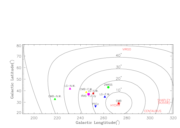
Figure 7: The triangles show the dipole directions at 13000 ${\rm\thinspace km}{\rm\thinspace s}^{-1}$derived in this paper. The direction of the number weighted 2MRS dipole in the LG frame is shown in magenta (LG-N.W., $l=231^{\circ}$, $b=42^{\circ}$). The red triangle shows the direction of the flux weighted 2MRS in the LG frame (LG-F.W., $l=251^{\circ}$, $b=38^{\circ}$). The blue triangle shows the direction of the flux weighted 2MRS in the LG frame excluding Maffei 1, Maffei 2, M81, IC342 and Dwingeloo 1 (LG-F.W., $l=261^{\circ}$, $b=35^{\circ}$). The red star shows the CMB dipole direction ($l=273^{\circ}$, $b=29^{\circ}$). The green triangle is the number weighted LG dipole in the CMB frame (CMB-N.W., $l=218^{\circ}$, $b=33^{\circ}$); the yellow triangle is the flux weighted LG dipole in CMB frame (CMB-F.W., $l=245^{\circ}$, $b=39^{\circ}$). The green circle is the 2MASS dipole ($l=264^{\circ}$, $b=43^{\circ}$, Maller et al. 2003). The magenta square is the $IRAS$ 1.2-Jy dipole ($l=247^{\circ}$, $b=37^{\circ}$, Webster et al. 1997). The blue upside-down triangle is the $IRAS$ PSCz dipole ($l=253^{\circ}$, $b=26^{\circ}$, Rowan-Robinson et al. 2000). Contours are drawn at constant misalignment angles. Also shown are the Virgo Cluster ($l=280^{\circ}$, $b=75^{\circ}$), the Hydra Cluster ($l=270^{\circ}$, $b=27^{\circ}$), the Centaurus Cluster ($l=302^{\circ}$, $b=22^{\circ}$) and A3558 ($l=312^{\circ}$, $b=31^{\circ}$).

The results are presented in Figures 6-7. The top plots of Figures 6-6 show the amplitudes and three spatial components of the acceleration on the Local group (top) and the convergence of the angle between the LG dipole and the CMB dipole (bottom) as a function of distance in two reference frames. For these plots, the galaxies in the masked regions are interpolated from the adjacent regions (Method 2). The right panel in each figure shows the results for the flux weighted dipole and the left panels show the results for the number weighted dipole. Figure 6 is for the the Local Group Frame and Figure 6 is in the CMB frame. As discussed in the next section, the results for the filling Method 1 where the galaxies are sampled randomly do not look very different than the results in Figures 6 & 6 and thus are not shown. Figure 7 compares the direction of the LG dipole estimate to that of the CMB and other LG dipole measurements.

We give the results for the flux weighted dipole calculated using the second method of mask filling in Table LABEL:tab:tab2. Column 1 is the radii of the concentric spheres within which the values are calculated; columns 2 and 3 are the amplitude of the velocity vector and the shot noise divided by ${\Omega_{\rm m}}^{0.6}/b_{\rm L}$, respectively; Columns 4, 5 and 6 show the direction of the velocity vector and its angle to the CMB dipole. The first line gives the results in the LG frame and the second line gives the results in CMB frame. Table LABEL:tab:tab3 is structured in the same way as Table LABEL:tab:tab2 however the analysis excludes five galaxies.

4.1 The Tug of War

In Figures 6 & 6, the LG velocity is dominated by structure within a distance of 60 ${\rm\thinspace km}{\rm\thinspace s}^{-1}$(except for the CMB frame number weighted dipole where the contribution from the distant structure is over-estimated.). The ‘tug of war’ between the Great Attractor and the Perseus-Pisces is clearly evident. The dip in the velocity vector is an indication that the local flow towards the Great Attractor is counteracted by the Perseus-Pisces complex in the opposite direction. If we take out 420 galaxies in the Perseus-Pisces ridge (defined by $-40\leq b\leq-10$, $110\leq b\leq 130$, 4600 ${\rm kms}^{-1}\leq cz\leq$ 6000 ${\rm kms}^{-1}$) and recalculate the convergence, the dip almost disappears and the convergence is dominated by the Great Attractor. This leads us to conclude that the Perseus-Pisces plays a significant role in the gravitational acceleration of the LG.

4.2 Filling the Zone of Avoidance

The choice of method used to fill the masked regions does not have much effect on the results. The convergence of the misalignment angle for the second method is slightly more stable than the first method and the overall direction of the LG dipole is closer to the CMB dipole. Since the Galactic $z$ component is least affected by the zone of avoidance, the discrepancy between the amplitudes in each plot comes mainly from the Galactic $x$ and $y$ components. The direction of the dipole is 2^∘-3^∘ closer to the CMB vector for the second method at distances where the Great Attractor lies. Of course, one cannot rule out the possibility that there may be important contribution to the dipole from other structures behind the zone of avoidance. The Great Attractor is most likely centred on the Norma Cluster ($l\approx$325^∘, $b\approx$-7^∘, Kraan-Korteweg et al. 1996) which lies very close to the obscured plane. Although, the 2MRS samples the Norma cluster much better than the optical surveys, the latitude range $|b|\lesssim 5$ which is still obscured in the 2MRS may have structure that play an important role in the dipole determinations. In fact, Scharf et al. (1992) and Lahav et al. (1993) point out that there is significant contribution to the local flow by the Puppis complex at low galactic latitudes that are not sampled by the 2MRS.

Kraan-Korteweg & Lahav (2000) point out that since the dipole is dominated by local structures, the detection of nearby galaxies can be more important to the dipole analyses than the detection of massive clusters at larger distances. We test this by excluding the five most luminous nearby galaxies (Maffei 1, Maffei 2, IC342, Dwingeloo 1 and M81) from our analysis. Remarkably, the direction of the resultant dipole moves much closer to that of the CMB (see Table LABEL:tab:tab3). All of these galaxies expect M81 lie very close to the Zone of Avoidance and they are excluded from most dipole analyses either because they are not in the catalogue (e.g. Rowan-Robinson et al. 2000) or they are masked out (e.g. Maller et al. 2003). In fact, when we change our mask to match that of Maller et al. (2003) and keep M81 in the analysis our resulting dipole is only 3^∘ degrees away from the dipole calculated by Maller et al. (2003). This illustrates the importance of the nearby structure behind the Zone of Avoidance.

The comparison of Tables LABEL:tab:tab2 and LABEL:tab:tab3 also highlights the vital role non-linear dynamics induced by nearby objects play in dipole calculations. Maller et al. (2003) investigate the non-linear contribution to the LG dipole by removing the bright galaxies with $K_{s}<8$. They report that the LG dipole moves to within a few degrees of the CMB dipole. They repeat their calculations for the PSCz survey and observe the same pattern. We do not observe this behaviour. When we remove the objects brighter that $K_{s}=8$ (428 galaxies), the misalignment angle of the resulting dipole decreases by $3^{\circ}$ for the flux weighted dipole and remains the same for the number weighted case. The dipole amplitudes decreases substantially in both cases, notably in the case of the flux dipole, suggesting that the brightest 2MRS galaxies play a significant role in inducing the LG velocity.

4.3 The Choice of Reference Frames

The number weighted LG dipole looks very different in different reference frames (Figures 6 and 6) whereas the flux weighted dipole is almost unaffected by the change. The number weighted dipole is similar to the flux weighted dipole in the LG frame. Thus, we conclude that it is more accurate to use the LG frame redshifts than that of the CMB frame.

4.4 The Choice of Weighting Schemes

The amplitudes of the number weighted LG dipole and the flux weighted LG dipole are very similar in the LG frame. However, the convergence of the misalignment angles of the flux and the number dipoles is quite different in both frames, especially at large distances. The angle of the flux weighted dipole is closer to the CMB dipole than its number weighted counterpart at all distances. With either weighting scheme, the dipoles are closest to the CMB dipole at a distance of about 5000 ${\rm\thinspace km}{\rm\thinspace s}^{-1}$and move away from the CMB dipole direction further away. However, the change in the direction of the flux weighted dipole is much smaller compared to the number weighted dipole and there is convergence within the error bars by 6000 ${\rm\thinspace km}{\rm\thinspace s}^{-1}$. The misalignment angles in the LG frame at 130 $h^{-1}$ Mpc are 21^∘ and $37^{\circ}$ for the flux and the number dipoles, respectively. The discrepancy is probably mainly due to the fact the number dipole is plagued with errors due to the lack of peculiar velocity information. In fact, when we use just the redshift information instead of the distance measurements (see Section 2.4) the number dipole moves $\approx 7^{\circ}$ towards the CMB dipole. The flux dipole assumes that the mass traces light whereas the number dipole assumes that all galaxies have the same mass. The former assumption is of course more valid, however, since the amplitudes of the dipoles are so similar in the LG frame, we conclude that the equal mass assumption for the number weighted dipole do not introduce large errors and that the discrepancy results from the errors in distance.

In all figures, $v_{x}$ and $v_{y}$ change with distance more rapidly in the number weighted scheme than the flux weighted. At further distances, the flux weighted $v_{x}$ flattens whereas its number weighted counterpart continues to grow. It is expected that the $(x,y)$ directions are particularly sensitive to the shape of the zone of avoidance, although it is not obvious why the flux weighted components remain so robust. Assuming the dipole has converged we can obtain values for ${\Omega_{\rm m}}^{0.6}/b$ (number weighted) and ${\Omega_{\rm m}}^{0.6}/b_{\rm L}$ (flux weighted) by comparing the amplitude of our dipole estimates to the CMB dipole. These values are summarised in Table 1. The values are quoted in the LG frame at 13000 ${\rm\thinspace km}{\rm\thinspace s}^{-1}$using the second mask and with the luminosity density value derived earlier, $\rho_{L}=7.67\pm 1.02\times 10^{8}$ $\rm\thinspace L_{\odot}$$h{\rm Mpc}^{-3}$. The errors take the shot noise, the uncertainties in the CMB dipole and $\rho_{L}$ (for the flux limited case) into account. The $\beta$ values obtained for the two different weighting schemes are in excellent agreement suggesting that the dark matter haloes are well sampled by the survey. Our value for $\beta$ is also in good agreement with results from 2MASS (Pike & Hudson 2005) and IRAS surveys (e.g. Zaroubi et al. 2002, Willick & Strauss 1998). In order to calculate the uncertainties introduced by the errors in the galaxy redshifts, ten realisations of the 2MRS catalogue are created with each galaxy redshift drawn from a Gaussian distribution with standard deviation equal to its error. It is found that the scatter in the dipole results due to the errors in redshifts are very small compared to the shot noise errors and thus are not quoted.

Table 1: The values derived for ${\Omega_{\rm m}}$, $\beta$.

${\Omega_{\rm m}}^{0.6}/b_{\rm L}$ from the flux weighted scheme	$=$	$0.40\pm 0.09$
${\Omega_{\rm m}}^{0.6}/b$ from the number weighted scheme	$=$	$0.40\pm 0.08$

4.5 The Milky Way Dipole

We also investigate the acceleration on our galaxy due to other eight members of the LG excluded from the LG dipole analysis. As expected, the flux dipole is strongly dominated by Andromeda (M31) with an amplitude of ${\rm v}/\beta\approx 220$${\rm\thinspace km}{\rm\thinspace s}^{-1}$directly towards M31 ($l\approx 121.4^{\circ},b\approx-21.7^{\circ}$), confirming that near-infrared fluxes are good tracers of mass. The number weighted dipole which assumes that the galaxies have the same weight gives a similar amplitude of ${\rm v}/\beta\approx 190$${\rm\thinspace km}{\rm\thinspace s}^{-1}$but its direction ($l\approx 104.6^{\circ},b\approx-21.6^{\circ}$) is skewed towards NGC 6822 ($l\approx 25.3^{\circ},b\approx-18.4^{\circ}$) which lies further away from the other seven galaxies that are grouped together.

Table 2: The convergence values calculated for flux weighted dipole using the second method for the masked region. The columns give (i)Radius of the concentric spheres within which the values are calculated; (ii) and (iii) amplitude of the velocity vector and the shot noise divided by $f(\Omega_{\rm m})$, respectively; (iv), (v) and (vi) direction of the velocity vector and its angle to the CMB dipole. The results in the first and second line are given in LG and CMB frames, respectively.

Dist	$V_{tot}b_{L}/f(\Omega_{\rm m})$	l	b	$\delta\theta$
km $s^{-1}$	km $s^{-1}$	deg	deg	deg
1000	590 $\pm$294	259${}^{\circ}\pm$ 59 ∘	39${}^{\circ}\pm$20 ∘	42${}^{\circ}\pm$20 ∘
	362 $\pm$289	331${}^{\circ}\pm$171 ∘	23${}^{\circ}\pm$23 ∘	99${}^{\circ}\pm$26 ∘
2000	1260 $\pm$318	249${}^{\circ}\pm$ 17 ∘	41${}^{\circ}\pm$13 ∘	25${}^{\circ}\pm$11 ∘
	993 $\pm$316	222${}^{\circ}\pm$ 22 ∘	41${}^{\circ}\pm$15 ∘	44${}^{\circ}\pm$15 ∘
3000	1633 $\pm$322	260${}^{\circ}\pm$ 12 ∘	40${}^{\circ}\pm$10 ∘	17${}^{\circ}\pm$ 8 ∘
	1334 $\pm$320	241${}^{\circ}\pm$ 17 ∘	44${}^{\circ}\pm$13 ∘	31${}^{\circ}\pm$11 ∘
4000	1784 $\pm$323	264${}^{\circ}\pm$ 10 ∘	39${}^{\circ}\pm$ 9 ∘	14${}^{\circ}\pm$ 7 ∘
	1513 $\pm$322	252${}^{\circ}\pm$ 14 ∘	41${}^{\circ}\pm$11 ∘	22${}^{\circ}\pm$ 9 ∘
5000	1838 $\pm$324	265${}^{\circ}\pm$ 10 ∘	36${}^{\circ}\pm$ 9 ∘	12${}^{\circ}\pm$ 7 ∘
	1497 $\pm$323	252${}^{\circ}\pm$ 13 ∘	39${}^{\circ}\pm$11 ∘	22${}^{\circ}\pm$ 9 ∘
6000	1633 $\pm$325	259${}^{\circ}\pm$ 10 ∘	34${}^{\circ}\pm$ 9 ∘	15${}^{\circ}\pm$ 8 ∘
	1438 $\pm$324	250${}^{\circ}\pm$ 12 ∘	36${}^{\circ}\pm$11 ∘	22${}^{\circ}\pm$ 9 ∘
7000	1682 $\pm$325	256${}^{\circ}\pm$ 10 ∘	36${}^{\circ}\pm$ 9 ∘	18${}^{\circ}\pm$ 8 ∘
	1503 $\pm$324	247${}^{\circ}\pm$ 12 ∘	36${}^{\circ}\pm$10 ∘	24${}^{\circ}\pm$ 9 ∘
8000	1697 $\pm$326	255${}^{\circ}\pm$ 11 ∘	37${}^{\circ}\pm$10 ∘	18${}^{\circ}\pm$ 8 ∘
	1566 $\pm$325	248${}^{\circ}\pm$ 12 ∘	39${}^{\circ}\pm$10 ∘	24${}^{\circ}\pm$ 9 ∘
9000	1683 $\pm$326	255${}^{\circ}\pm$ 11 ∘	38${}^{\circ}\pm$10 ∘	19${}^{\circ}\pm$ 8 ∘
	1573 $\pm$325	248${}^{\circ}\pm$ 12 ∘	39${}^{\circ}\pm$10 ∘	24${}^{\circ}\pm$ 9 ∘
10000	1674 $\pm$326	253${}^{\circ}\pm$ 11 ∘	38${}^{\circ}\pm$10 ∘	20${}^{\circ}\pm$ 8 ∘
	1599 $\pm$325	246${}^{\circ}\pm$ 12 ∘	39${}^{\circ}\pm$10 ∘	26${}^{\circ}\pm$ 8 ∘
11000	1677 $\pm$326	253${}^{\circ}\pm$ 11 ∘	38${}^{\circ}\pm$10 ∘	21${}^{\circ}\pm$ 8 ∘
	1624 $\pm$325	246${}^{\circ}\pm$ 12 ∘	40${}^{\circ}\pm$10 ∘	26${}^{\circ}\pm$ 8 ∘
12000	1676 $\pm$326	253${}^{\circ}\pm$ 11 ∘	38${}^{\circ}\pm$10 ∘	21${}^{\circ}\pm$ 8 ∘
	1624 $\pm$325	246${}^{\circ}\pm$ 12 ∘	40${}^{\circ}\pm$10 ∘	26${}^{\circ}\pm$ 8 ∘
13000	1652 $\pm$326	251${}^{\circ}\pm$ 11 ∘	38${}^{\circ}\pm$10 ∘	21${}^{\circ}\pm$ 8 ∘
	1629 $\pm$325	245${}^{\circ}\pm$ 12 ∘	39${}^{\circ}\pm$10 ∘	26${}^{\circ}\pm$ 8 ∘
14000	1659 $\pm$327	251${}^{\circ}\pm$ 11 ∘	38${}^{\circ}\pm$10 ∘	22${}^{\circ}\pm$ 8 ∘
	1636 $\pm$326	245${}^{\circ}\pm$ 11 ∘	39${}^{\circ}\pm$10 ∘	26${}^{\circ}\pm$ 8 ∘
15000	1640 $\pm$327	251${}^{\circ}\pm$ 11 ∘	37${}^{\circ}\pm$10 ∘	21${}^{\circ}\pm$ 8 ∘
	1633 $\pm$326	246${}^{\circ}\pm$ 11 ∘	39${}^{\circ}\pm$10 ∘	25${}^{\circ}\pm$ 8 ∘
16000	1638 $\pm$327	251${}^{\circ}\pm$ 11 ∘	37${}^{\circ}\pm$10 ∘	21${}^{\circ}\pm$ 8 ∘
	1643 $\pm$326	247${}^{\circ}\pm$ 11 ∘	38${}^{\circ}\pm$10 ∘	25${}^{\circ}\pm$ 8 ∘
17000	1630 $\pm$327	251${}^{\circ}\pm$ 11 ∘	37${}^{\circ}\pm$10 ∘	21${}^{\circ}\pm$ 8 ∘
	1643 $\pm$326	247${}^{\circ}\pm$ 11 ∘	38${}^{\circ}\pm$10 ∘	25${}^{\circ}\pm$ 8 ∘
18000	1604 $\pm$328	251${}^{\circ}\pm$ 11 ∘	37${}^{\circ}\pm$10 ∘	21${}^{\circ}\pm$ 8 ∘
	1631 $\pm$327	247${}^{\circ}\pm$ 11 ∘	38${}^{\circ}\pm$10 ∘	25${}^{\circ}\pm$ 8 ∘
19000	1591 $\pm$328	251${}^{\circ}\pm$ 11 ∘	37${}^{\circ}\pm$10 ∘	21${}^{\circ}\pm$ 8 ∘
	1629 $\pm$327	247${}^{\circ}\pm$ 11 ∘	38${}^{\circ}\pm$10 ∘	24${}^{\circ}\pm$ 8 ∘
20000	1577 $\pm$328	251${}^{\circ}\pm$ 12 ∘	37${}^{\circ}\pm$10 ∘	21${}^{\circ}\pm$ 8 ∘
	1620 $\pm$327	247${}^{\circ}\pm$ 11 ∘	37${}^{\circ}\pm$10 ∘	24${}^{\circ}\pm$ 8 ∘

Table 3: Same as Table LABEL:tab:tab2 but the analysis excludes the galaxies: Maffei 1, Maffei 2, Dwingeloo 1, IC342 and M81.

Dist	$V_{tot}b_{L}/f(\Omega_{\rm m})$	l	b	$\delta\theta$
km $s^{-1}$	km $s^{-1}$	deg	deg	deg
1000	585 $\pm$254	280${}^{\circ}\pm$ 30 ∘	34${}^{\circ}\pm$17 ∘	25${}^{\circ}\pm$ 9 ∘
	181 $\pm$228	360${}^{\circ}\pm$108 ∘	24${}^{\circ}\pm$29 ∘	67${}^{\circ}\pm$37 ∘
2000	1258 $\pm$282	263${}^{\circ}\pm$ 13 ∘	38${}^{\circ}\pm$11 ∘	15${}^{\circ}\pm$ 9 ∘
	963 $\pm$261	259${}^{\circ}\pm$ 18 ∘	39${}^{\circ}\pm$13 ∘	19${}^{\circ}\pm$12 ∘
3000	1661 $\pm$285	269${}^{\circ}\pm$ 9 ∘	37${}^{\circ}\pm$ 9 ∘	11${}^{\circ}\pm$ 5 ∘
	1352 $\pm$266	265${}^{\circ}\pm$ 12 ∘	41${}^{\circ}\pm$10 ∘	16${}^{\circ}\pm$ 8 ∘
4000	1824 $\pm$287	272${}^{\circ}\pm$ 8 ∘	36${}^{\circ}\pm$ 8 ∘	10${}^{\circ}\pm$ 4 ∘
	1571 $\pm$268	269${}^{\circ}\pm$ 9 ∘	37${}^{\circ}\pm$ 9 ∘	12${}^{\circ}\pm$ 5 ∘
5000	1891 $\pm$288	272${}^{\circ}\pm$ 8 ∘	33${}^{\circ}\pm$ 7 ∘	8${}^{\circ}\pm$ 3 ∘
	1559 $\pm$270	268${}^{\circ}\pm$ 9 ∘	35${}^{\circ}\pm$ 8 ∘	10${}^{\circ}\pm$ 5 ∘
6000	1678 $\pm$289	268${}^{\circ}\pm$ 8 ∘	31${}^{\circ}\pm$ 8 ∘	9${}^{\circ}\pm$ 4 ∘
	1504 $\pm$271	266${}^{\circ}\pm$ 9 ∘	32${}^{\circ}\pm$ 8 ∘	10${}^{\circ}\pm$ 5 ∘
7000	1713 $\pm$289	264${}^{\circ}\pm$ 8 ∘	33${}^{\circ}\pm$ 8 ∘	11${}^{\circ}\pm$ 6 ∘
	1551 $\pm$272	263${}^{\circ}\pm$ 9 ∘	33${}^{\circ}\pm$ 8 ∘	12${}^{\circ}\pm$ 6 ∘
8000	1721 $\pm$290	264${}^{\circ}\pm$ 9 ∘	35${}^{\circ}\pm$ 8 ∘	11${}^{\circ}\pm$ 7 ∘
	1611 $\pm$272	264${}^{\circ}\pm$ 9 ∘	36${}^{\circ}\pm$ 8 ∘	12${}^{\circ}\pm$ 7 ∘
9000	1704 $\pm$290	264${}^{\circ}\pm$ 9 ∘	35${}^{\circ}\pm$ 8 ∘	12${}^{\circ}\pm$ 7 ∘
	1614 $\pm$272	264${}^{\circ}\pm$ 9 ∘	36${}^{\circ}\pm$ 8 ∘	12${}^{\circ}\pm$ 7 ∘
10000	1691 $\pm$290	262${}^{\circ}\pm$ 9 ∘	36${}^{\circ}\pm$ 8 ∘	13${}^{\circ}\pm$ 7 ∘
	1634 $\pm$272	262${}^{\circ}\pm$ 9 ∘	36${}^{\circ}\pm$ 8 ∘	13${}^{\circ}\pm$ 7 ∘
11000	1691 $\pm$290	262${}^{\circ}\pm$ 9 ∘	36${}^{\circ}\pm$ 8 ∘	13${}^{\circ}\pm$ 7 ∘
	1658 $\pm$273	262${}^{\circ}\pm$ 9 ∘	37${}^{\circ}\pm$ 8 ∘	14${}^{\circ}\pm$ 7 ∘
12000	1690 $\pm$291	262${}^{\circ}\pm$ 9 ∘	35${}^{\circ}\pm$ 8 ∘	13${}^{\circ}\pm$ 7 ∘
	1658 $\pm$273	261${}^{\circ}\pm$ 9 ∘	37${}^{\circ}\pm$ 8 ∘	14${}^{\circ}\pm$ 7 ∘
13000	1665 $\pm$291	261${}^{\circ}\pm$ 9 ∘	35${}^{\circ}\pm$ 9 ∘	14${}^{\circ}\pm$ 7 ∘
	1663 $\pm$273	261${}^{\circ}\pm$ 9 ∘	36${}^{\circ}\pm$ 8 ∘	14${}^{\circ}\pm$ 7 ∘
14000	1671 $\pm$291	260${}^{\circ}\pm$ 9 ∘	35${}^{\circ}\pm$ 8 ∘	14${}^{\circ}\pm$ 7 ∘
	1668 $\pm$273	260${}^{\circ}\pm$ 9 ∘	36${}^{\circ}\pm$ 8 ∘	14${}^{\circ}\pm$ 6 ∘
15000	1652 $\pm$291	260${}^{\circ}\pm$ 9 ∘	35${}^{\circ}\pm$ 9 ∘	14${}^{\circ}\pm$ 7 ∘
	1670 $\pm$274	261${}^{\circ}\pm$ 9 ∘	36${}^{\circ}\pm$ 8 ∘	13${}^{\circ}\pm$ 6 ∘
16000	1653 $\pm$292	261${}^{\circ}\pm$ 9 ∘	34${}^{\circ}\pm$ 9 ∘	13${}^{\circ}\pm$ 7 ∘
	1683 $\pm$274	261${}^{\circ}\pm$ 8 ∘	35${}^{\circ}\pm$ 8 ∘	13${}^{\circ}\pm$ 6 ∘
17000	1647 $\pm$292	261${}^{\circ}\pm$ 9 ∘	34${}^{\circ}\pm$ 8 ∘	13${}^{\circ}\pm$ 7 ∘
	1684 $\pm$274	261${}^{\circ}\pm$ 8 ∘	35${}^{\circ}\pm$ 8 ∘	13${}^{\circ}\pm$ 6 ∘
18000	1619 $\pm$292	260${}^{\circ}\pm$ 9 ∘	34${}^{\circ}\pm$ 9 ∘	14${}^{\circ}\pm$ 7 ∘
	1672 $\pm$274	261${}^{\circ}\pm$ 9 ∘	35${}^{\circ}\pm$ 8 ∘	13${}^{\circ}\pm$ 6 ∘
19000	1606 $\pm$292	260${}^{\circ}\pm$ 9 ∘	34${}^{\circ}\pm$ 9 ∘	14${}^{\circ}\pm$ 7 ∘
	1672 $\pm$274	262${}^{\circ}\pm$ 8 ∘	35${}^{\circ}\pm$ 8 ∘	13${}^{\circ}\pm$ 6 ∘
20000	1594 $\pm$293	261${}^{\circ}\pm$ 9 ∘	34${}^{\circ}\pm$ 9 ∘	13${}^{\circ}\pm$ 7 ∘
	1665 $\pm$275	262${}^{\circ}\pm$ 8 ∘	34${}^{\circ}\pm$ 8 ∘	12${}^{\circ}\pm$ 6 ∘

Figure 5: Top: Three components and the magnitudes of the acceleration of the Local Group due to galaxies within a series of successively larger concentric spheres centred on the local group in the Local Group frame. The galaxies in the masked regions are interpolated from the adjacent regions (Method 2). Left panel is the number weighted velocity and right panel is the flux weighted velocity. The growth of the estimated shot noise is also shown. Bottom: Convergence of the direction of the LG dipole where the misalignment angle is between the LG and the CMB dipoles. The dotted lines denote 1$\sigma$ errors from shot noise. Left plot is the direction of the number weighted LG dipole and right plot is the direction of the flux weighted LG dipole. We note for the number weighted dipole the dramatic increase in shot noise beyond 15000 ${\rm\thinspace km}{\rm\thinspace s}^{-1}$, where the dipole’s behaviour cannot be interpreted reliably.

Figure 6: Same as in Figure 6 but in CMB frame.

5 Discussion

In this paper, we calculate the 2MRS dipole using number and flux weighting schemes. The flux weighted dipole bypasses the effects of redshift space distortions and the choice of reference frames giving very robust results.

Our dipole estimates are dominated by the tug of war between the Great Attractor and the Perseus-Pisces superclusters and seemingly converge by 6000 ${\rm\thinspace km}{\rm\thinspace s}^{-1}$. The contribution from structure beyond these distances is negligible. The direction of the flux dipole (l=251${}^{\circ}\pm$12^∘,b=37${}^{\circ}\pm$ 10 ^∘) is in good agreement with the 2MASS dipole derived by Maller et al. (2003) (l=264.5${}^{\circ}\pm$2^∘,b=43.5${}^{\circ}\pm$ 4 ^∘). The difference in results is probably due to the fact that they use a higher latitude cutoff in the mask ($|b|<7^{\circ}$) and exclude all galaxies below this latitude. We confirm this by changing our treatment of the Zone of Avoidance to match theirs. We find that the flux dipole is very close to their dipole direction. Their limiting Kron magnitude is $K_{s}=13.57$ which corresponds to an effective depth of 200 $h^{-1}$ Mpc. As their sample is deep enough to pick out galaxies in the Shapley Supercluster, the comparison of their dipole value with our values suggests that the contribution to the LG dipole from structure further away than the maximum distance of our analysis is not significant. Following Maller et al. (2003), when we adopt $\Omega_{\rm m}=0.27$ we get $b_{L}=1.14\pm 0.25$, in good agreement with their value of $b=1.06\pm 0.17$ suggesting that the 2MRS galaxies are unbiased. We note that the 2MRS value for the linear bias is somewhat lower than expected considering that the 2MRS has a high proportion of early type galaxies which are known to reside mostly in high density regions (e.g. Norberg et al. 2001, Zehavi et al. 2002). The values we derive for $\beta$ and ${\Omega_{\rm m}}$ are consistent with the concordance $\Lambda$-CDM model values given their error bars.

Figure 3 shows that the 2MRS samples the Great Attractor region better than the PSCz survey but that the PSCz redshift distribution has a longer redshift tail than the 2MRS. Nevertheless, PSCz dipole agrees well with that of the 2MRS. Rowan-Robinson et al. (2000) derive a value for $\beta=0.75^{+0.11}_{-0.08}$ which is higher than the value we derive in this paper. The PSCz sample is biased towards star-forming galaxies and thus under-samples the ellipticals which lay in high density regions. Contrarily, the 2MRS is biased towards early-type galaxies. This difference may be the reason why they get a higher value for $\beta$. The flux weighted dipole is in excellent agreement with the $IRAS$ 1.2 Jy dipole (Webster, Lahav & Fisher 1997) which was obtained using a number weighted scheme but with an added filter that mitigates the shot noise and deconvolves redshift distortions. Our number weighted dipole differs from their results. This is probably due to fact that the 2MRS number weighted dipole is plagued wit redshift distortions. Webster, Lahav & Fisher (1997) obtain the real-space density field from that in the redshift-space using a Wiener Filter. In a forthcoming paper, we will use the same technique to address this issue. Similarly, the 2MRS number weighted dipole also differs from the PSCz dipole which was calculated using a flow model for massive clusters.

The analysis of the $IRAS$ QDOT galaxies combined with Abell clusters (Plionis, Coles & Catelan 1993) and the X-Ray cluster only dipole (Kocevski, Mullis & Ebeling 2004 and Kocevski & Ebeling 2005) imply a significant contribution to the LG velocity by the Shapley Supercluster. Kocevski & Ebeling (2005) report a significant contribution to the LG dipole (56%) from distances beyond 60 $h^{-1}$ Mpc. The discrepancy between their results and ours is possibly due to the fact that the 2MRS is a better tracer of the galaxies at nearby distances, whereas the X-ray cluster data are better samplers of the matter distribution beyond 150 $h^{-1}$ Mpc.

The misalignment angle between the LG and the CMB dipole is smallest at 5000 ${\rm\thinspace km}{\rm\thinspace s}^{-1}$where it drops to 12${}^{\circ}\pm$7^∘ and increases slightly at larger distances presumably due to shot-noise. This behaviour is also observed in the other dipole analyses (e.g. Webster, Lahav, Fisher 1997 & Rowan-Robinson et al. 2000). This is a strong indication that most of the LG velocity is due to the Great Attractor and the Perseus-Pisces superclusters. Of course, we still cannot rule out a significant contribution from Shapley as we do not sample that far. However, it may be more important ask what the velocity field in the Great Attractor region is. In other words, whether we observe a significant backside infall towards the Great Attractor.

The smallest misalignment angle at 13000 ${\rm\thinspace km}{\rm\thinspace s}^{-1}$is 21${}^{\circ}\pm$8^∘, found for the LG frame, flux weighted scheme using the second mask. This misalignment can be due to several effects:

• The analysis uses linear perturbation theory which is correct only to first order $\delta$. There may be contributions to the LG dipole from small scales which would cause gravity and the velocity vectors to misalign, even with perfect sampling. However, Ciecielag, Chodorowski & Kudlicki (2001) show that these non-linear effects cause only small misalignments for the $IRAS$ PSCz survey. However, removing the five most luminous nearby galaxies moves the flux dipole to ($l=261^{\circ}\pm 9^{\circ}$, $b=34^{\circ}\pm 9^{\circ}$,cz=20000 ${\rm\thinspace km}{\rm\thinspace s}^{-1}$), 8^∘ closer to that of the CMB. This suggests that the non-linear effects might be very important in dipole determinations.

• The sampling is not perfect and the selection effects of the surve will increase the shot noise-errors especially at large distances causing misalignments.

• There may be uncertainties in the assumptions in galaxy formation and clustering. For example the mass-to-light ratios might differ according to type and/or vary with luminosity or the galaxy biasing might be non-linear and/or scale dependent.

• There may be a significant contribution to the LG dipole from structure further away than the maximum distance of our analysis.

• The direction of the LG dipole may be affected by nearby galaxies at low latitudes which are not sampled by the 2MRS. In the future, the masked regions will be filled by galaxies from other surveys such as the ongoing HI Parkes Deep Zone of Avoidance Survey (Henning et al. 2004) as well as the galaxies that are sampled from the 2MRS itself.

Our initial calculations of the expected LG acceleration (c.f. Lahav, Kaiser & Hoffman 1990; Juszkiewicz, Vittorio & Wyse 1990) suggest that the misalignment of 21${}^{\circ}\pm$8^∘ is within 1 $\sigma$ of the dipole probability distribution in a CDM Universe with $\Omega_{\rm m}=0.3$. In a forthcoming paper, the cosmological parameters will be constrained more vigourously using a maximum likelihood analysis based on the spherical harmonics expansion (e.g. Fisher, Scharf & Lahav 1994; Heavens & Taylor 1995) of the 2MRS density field.

References

- [1] Bell E.F. & de Jong R.S., 2001, ApJ, 550, 212
- [2] Bennett C.L., et al. , 2003, ApJS, 148, 1
- [3] Branchini E. & Plionis M., 1996, ApJ, 460, 569
- [4] Brunozzi P.T., Borgani S., Plionis M., Moscardini L. & Coles P., 1995, MNRAS, 277, 1210
- [5] Cambresy L., Jarrett T.H. & Beichman C.A., 2005, A&A,435, 131
- [6] Cardelli J.A., Clayton G.C. & Mathis J.S., 1989, ApJ, 345, 245
- [7] Ciecielag P., Chodorowski M. & Kudlicki A., 2001, Acta Astronomical, 51, 103
- [8] Cohen M., Wheaton W.A. & Megeath S.T., 2003, AJ, 126, 1090
- [9] Cole S. & the 2dFGRS team, 2001, MNRAS, 326, 255
- [10] Conklin E.K., Nature, 1969, 222, 971
- [11] Courteau S. & Van Den Bergh S., 1999, AJ, 118, 337
- [12] Cowie L.L., Gardner J.P., Hu E.M., Songaila A., Hodapp K.W. & Wainscoat R.J., 1994, ApJ, 434, 114
- [13] Davis M. & Huchra J.P., 1982, ApJ, 254, 437
- [14] da Costa L.N., et al. , 2000, ApJ, 537, L81
- [15] Fisher K.B., Scharf C.A. & Lahav O., 1994, MNRAS, 266, 219
- [16] Freedman W.L., et al., 2001, ApJ, 553, 47
- [17] Gunn J. E. 1988, in ASP Conf. Ser., Vol. 4, The Extragalactic Distance Scale, eds. S. van den Bergh & C. J. Pritchet (San Francisco: ASP), 344
- [18] Harmon R.T., Lahav O. & Meurs E.J.A., 1987, MNRAS, 228, 5
- [19] Huchra J.P. et al. , 2005, in preperation
- [20] Heavens A.F. & Taylor A.N., 1995, MNRAS, 275, 483
- [21] Henry P.S., 1971, Nature, 231, 516
- [22] Jarrett T.H., Chester T., Cutri R., Schneider S.E., Skrutsie M. & Huchra J.P., 2000, AJ, 119, 2498
- [23] Jarrett T.H., Chester T., Cutri R., Schneider S.E., Rosenberg J., & Huchra J.P., 2000, AJ, 120, 298
- [24] Jarrett T.H., Chester T., Cutri R., Schneider S.E. & Huchra J.P., 2003, AJ, 125, 525
- [25] Jarrett T.H., 2004, PASA, 21, 396
- [26] Jones D. H. & the 6dFGS Team, 2004, MNRAS, 355, 747
- [27] Juszkiewicz R., Vittorio N. & Wyse R.F.G., 1990, ApJ, 349, 408
- [28] Karachentsev I.D., Karachentseva V.E., Huchtmeier W. K., Makarov, D.I. 2004, AJ, 127, 2031
- [29] Kaiser N., 1987, MNRAS, 227, 1
- [30] Kaiser N. & Lahav 0., 1988, in Large-Scale Motions in the Universe, ed. V. C. Rubin & G. V. Coyne, Princeton University Press, p. 339
- [31] Kaiser N. & Lahav 0., 1989, MNRAS, 237, 129
- [32] Kochanek C.S., et al. , 2001, ApJ, 560, 566
- [33] Kocevski D.D., Mullis C.R. & Ebeling H., 2004, ApJ, 608, 721
- [34] Kocevski D.D. & Ebeling H., 2005, submitted to ApJ
- [35] Kraan-Korteweg R.C., Woudt P.A., Cayatte V., Fairall F.P., Balkowski C. & Henning P.A., 1996, Nature, 379, 519
- [36] Kraan-Korteweg R.C. & Lahav O., 2000, A&ARv, 10, 211
- [37] Kraan-Korteweg R.C., 2005, Reviews in Modern Astronomy 18, ed. S. Röser, (New York: Wiley),48
- [38] Lahav O., 1987, MNRAS, 225, 213
- [39] Lahav O., Rowan-Robinson M. & Lynden-Bell, 1988, MNRAS, 234, 677
- [40] Lahav O., Kaiser N. & Hoffman Y., 1990, ApJ, 352, 448
- [41] Lahav O., Lilje P.B., Primack J.R. & Rees M., 1991, MNRAS, 251, 128
- [42] Lahav O., Yamada T., Scharf C. & Kraan-Korteweg R.C., 1993, MNRAS, 262, 711
- [43] Lahav O., Fisher K.B., Hoffman Y., Scharf C.A. & Zaroubi S., 1994, ApJ, 423, 93
- [44] Lanzoni B., Ciotti L., Cappi A., Tormen G. & Zamorani G., 2004, ApJ, 600, 640
- [45] Lynden-Bell D., Lahav O. & Burstein D., 1989, MNRAS, 241,325
- [46] Maller A.H., McIntosh D.H., Katz N. & Weinberg M.D., 2003, ApJ, 598, L1
- [47] Maller A.H., McIntosh D.H., Katz N. & Weinberg M.D., 2005, ApJ, 619, 147
- [48] Meiksin A. & Davis M., 1986, AJ, 91, 191
- [49] Norberg P. & the 2dFGRS Team, 2001, MNRAS, 328, 64
- [50] Paczyński B. & Piran T., 1990, ApJ, 364, 341
- [51] Peebles P.J.E., 1980, The Large-Scale Structure of the Universe, Princeton University Press, Princeton
- [52] Pike R.W. & Hudson M.J., 2005, ApJ, in press
- [53] Plionis M., Coles P. & Catelan P., 1993, MNRAS, 262, 465
- [54] Rowan-Robinson M., et al. 2000, MNRAS, 314, 375
- [55] Saunders W., et al. , 2000, MNRAS, 317, 55
- [56] Scaramella R., Vettolani G. & Zamorani G., 1991, ApJ, 376, L1
- [57] Scharf C.A., Hoffman Y., Lahav O. & Lynden-Bell D., 1992, MNRAS, 256, 229
- [58] Schlegel D.J., Finkbeiner D.P. & Davis M., 1998, ApJ, 500, 525
- [59] Schmoldt I.M., et al. , 1999, MNRAS, 304, 893
- [60] Strauss M.A., Yahil A., Davis M., Huchra J.P. & Fisher K., 1992, ApJ, 397, 395
- [61] Villumsen J.V. & Strauss M.A., 1987, ApJ, 322, 37
- [62] Webster M., Lahav O. & Fisher K., 1997, MNRAS, 287,425
- [63] Willick J.A. & Strauss M.A., 1998, ApJ, 507, 64
- [64] Worthey G., 1994, ApJS, 95, 107
- [65] Yahil A., Sandage A. & Tammann G.A., 1980, ApJ, 242, 448
- [66] Yahil A., Walker D. & Rowan-Robinson M., 1986, ApJ, 301, L1
- [67] Yahil A., Strauss M., Davis M. & Huchra J.P., 1991, ApJ, 372, 393
- [68] Zaroubi S., Branchini E., Hoffman Y. & da Costa L.N., 2002, MNRASm 336, 1234
- [69] Zehavi I. & the SDSS Team, 2002, ApJ, 571, 172