Non-Gaussianity in the WMAP data using the peak-peak correlation function

Abstract

We present a search for non-Gaussianity in the WMAP first-year data using the two-point correlation function of maxima and minima in the temperature map. We find evidence for non-Gaussianity on large scales, whose origin appears to be associated with unsubstracted foregrounds, but which is not entirely clear. The signal appears to be associated most strongly with cold spots, and is more pronounced in the Southern galactic hemisphere. Removal of the region of sky near the galactic plane, or filtering out large-scale modes removes the signal. Analysis of individual frequency maps shows strongest signal in the 41GHz Q band. A study of difference maps tests the hypothesis that the non-Gaussianity is due to residual foregrounds and noise, but shows no significant detection. We suggest that the detection is due to large-scale residual foregrounds affecting more than one frequency band, but a primordial contribution from the Cosmic Microwave Background cannot be excluded.

Non-Gaussianity in the WMAP data using the peak-peak correlation function

1 Introduction

The hypothesis of primordial statistical random Gaussianity lies at the core of our understanding of the Universe. The currently favoured standard cosmological model is built upon the assumption of a set of initial conditions laid down during Inflation (Guth, 1981). In the most simple model of Inflation, these initial conditions produce nearly Gaussian temperature fluctuations of the Cosmic Microwave Background (CMB). If the CMB temperature field is indeed Gaussian distributed, its two-point angular correlation function (or power spectrum in dual space) contains all the information needed to characterise its statistical properties fully. In the Inflation paradigm and the hypothesis of statistical isotropy (i.e. invariance under rotations of n-point correlation functions), the angular power spectrum $C_{\ell}$ naturally became the standard statistical tool from which to extract all the cosmological information present in the CMB data (Jungman et al., 1996). If, on the contrary, the microwave background radiation is significantly non-Gaussian, it would be powerful evidence against Inflation with far-reaching consequences for our understanding of structure formation.

As a consequence, testing the precise statistical nature of the CMB anisotropies is of extreme importance in order to test the validity of our present theories of structure formation and of our current methods of parameter estimation. These statistical tests are complicated by the inevitable presence of foregrounds, such as the emission from our own galaxy or extra-galactic point sources and systematic and instrumental effects which may introduce spurious non-Gaussianities in the measurements. At small angular scales, secondary anisotropies such as the Sunyaev-Zel’dovich effect (Sunyaev & Zeldovich, 1972), the Ostriker-Vishniac effect (Ostriker & Vishniac, 1986; Castro, 2003), the Rees-Sciama effect (Rees & Sciama, 1968) and lensing by intervening structures (Blanchard & Schneider, 1987; Hu, 2001; Cooray & Kesden, 2003) as well as cross correlations between them (Cooray & Hu, 2000; Cooray, 2001a, b; Komatsu, 2001; Verde & Spergel, 2002) will also leave their own non-Gaussian signatures; these a valuable source of cosmological and astrophysical information in their own right.

Due to the scientific importance of measuring any non-Gaussianity, but also to the difficulty of detecting it, many non-Gaussianity studies have been performed at various angular scales since the first CMB measurements by the Cosmic Background Explorer (COBE) satellite (Smoot et al., 1992). Remarkably COBE provided the first non-Gaussianity detection by means of the bispectrum (Ferreira, Magueijo & Górski, 1998; Heavens, 1998), a detection that was later claimed to be due to undocumented systematic effects (Banday, Zaroubi & Górski, 2000; Magueijo, 2000; Magueijo & Medeiro, 2004). With the advent of higher sensitivity and higher resolution experiments, in particular the Wilkinson Microwave Anisotropy Probe (WMAP;  Bennett et al. 2003), with its low noise and large sky coverage, the pursuit of non-Gaussianity has become one of the main objectives of the CMB field.

As non-Gaussianity can take innumerable forms, it is difficult to test its presence and there is no optimal general test for detecting and quantifying it. Different tests can show higher or lower sensitivity depending on the type of non-Gaussianity being tested (see e.g.  Aghanim et al. (2003)). Clearly, it is important to apply as many different estimators as possible as the eventual understanding of any deviation from Gaussianity will likely come from a combination of complementary results.

A multitude of non-Gaussian estimators have thus been applied to the WMAP first year data such as the bispectrum, Minkowski functionals, three-point angular correlation function, higher-order moments of the angular correlation function, wavelets, phase correlations, tensor modes etc. (Colley & Gott, 2003; Komatsu et al., 2003; Park, 2004; Vielva et al., 2004; Coles et al., 2004; Copi, Huterer & Starkman, 2004; Cruz et al., 2005; Eriksen et al., 2004a, b, 2005; Land & Magueijo, 2005b, c; McEwen et al., 2005; Mukherjee & Wang, 2004; Gurzadyan et al., 2005; Jaffe et al., 2005; Land & Magueijo, 2005a; Liu & Zhang, 2005). Curiously, the data consistently show a variety of anomalies. The first of them concerns the low value of the quadrupole (multipole $\ell=2$), previously observed in the COBE data and whose origin has been discussed in terms of super-horizon fluctuations and spatial curvature e.g. Berera, Fang & Hinshaw (1998); Berera & Heavens (2000); Efstathiou (2003). Subsequently, studies indicated an unusual low probability planarity and alignment of the quadrupole and of the octopole ($\ell=3$), maybe even extending to higher multipole values ($\ell=5$). In addition, an analysis performed with Spherical Mexican Hat Wavelets (Cruz et al., 2005) provided the detection of a very non-Gaussian structure in the data, associated to a cold spot of around $10$ degrees, visible in the WMAP temperature maps. Last but not least, the data appear to exhibit a North-South asymmetry on large scales. Notoriously, all these claims indicate not only a deviation from the Gaussianity hypothesis but most alarming a violation of statistical isotropy, one of the two fundamental pillars – together with statistical homogeneity– of the Cosmological Principle. A plausible explanation for these surprising results is likely to be simply the presence of unaccounted systematics. But one cannot put aside the possibility of there being of cosmological origin, in which case it would have far-reaching consequences for our perception of the Universe and thus for the standard Cosmological model.

The peak-peak correlation function of a Gaussian random field has been calculated exactly, both in the full-sky and in the flat-sky approximation, and depends, as it must, only on the power spectrum (Heavens & Sheth, 1999; Heavens & Gupta, 2001). It has been shown to display a rich structure, in particular at small angular scales, raising the hope that it has a good sensitivity to a global non-Gaussian signal. The present study uses an estimator of the 2-point correlation function of the temperature hot spots (local maxima) and cold spots (local minima) to look for any deviation from the Gaussian hypothesis in the WMAP first-year temperature data. Following the claims of a North-South asymmetry, we also analyse both hemispheres separately.

This paper is organised as follows. In Section 2 and 3 we explain in detail our methodology, including the map construction pipeline, the peak-peak correlation function estimator used and the statistical method chosen to test robustly the Gaussianity of the data. In Section 4 we apply our method to the WMAP first year maps and present our results. In order to test various statistical properties of the whole data, we performed a full-sky study and a North-South comparison analysis of a map resulting from combining all the different frequency assemblies maps provided by WMAP. In particular we investigated how this North-South comparison changes with cuts both in harmonic and real space. To further test for the origin of any non-Gaussianity, we present both a full-sky and a North-South analysis performed on single-frequency maps and on frequency-difference maps, which removes the primordial signal and tests noise and residual foregrounds. Finally, in Section 5 we present our conclusions.

2 Method

The two-point correlation function of peaks of a Gaussian random field can be calculated analytically, given only its power spectrum  (Heavens & Gupta, 2001).

The power spectrum has been estimated from the WMAP data (Hinshaw et al., 2003), and we test the hypothesis that the field giving rise to this power spectrum is Gaussian. We do this by taking a brute force approach and use the best-fit $\Lambda$CDM theoretical power spectrum to the WMAP data as the starting point to generate a large number of Gaussian maps at all WMAP frequencies, to which we then apply sky cuts, window functions and noise so as to mimic the real data.

In this way, we estimate the hot spot and cold spot correlation functions, and their covariance, for the Gaussian maps created with the same algorithm as the real data. We then use these to test the Gaussian hypothesis.

2.1 The maps

2.1.1 The WMAP map

The WMAP satellite probed the CMB at five different frequencies with two radiometers, producing ten differencing assemblies (DAs): four on the W-band (94GHz), two on the V-band (61GHz), two on the Q-band (41GHz), one on the Ka-band (33GHz) and one on the K-band (23GHz). Each of these assemblies, after calibration and removal of the monopole and dipole, is available for download from the WMAP web-site. All the maps are provided in the Hierarchical Equal Area isoLatitude Pixelisation (HEALPix) scheme, which has proved to have several advantages over other methods of pixelising the surface of a sphere, in particular the fact that the pixel area is kept constant throughout the surface of the sphere. However, the pixel shapes can vary largely between the equatorial and polar regions and distance between pixel centres is not kept constant. The HEALPix scheme divides the sphere surface into 12 faces of 4 sides each, giving a minimum resolution of 12 pixels. Each side is divided in $N_{side}$ pixels, giving a total number of pixels in a map of $12N_{side}^{2}$. The WMAP maps were provided at a resolution of $N_{side}=512$ giving a total of 3,145,728 pixels separated on average by $\theta_{pix}=0.115$ degrees $=6.87$ arc minutes.

Each DA map pixel $p$ contains the temperature field (in mK) and a field containing the number of observations, $N_{obs}(p)$, which allows the noise per pixel to be estimated using

$$\sigma(p)=\frac{\sigma_{0}}{\sqrt{N_{obs(p)}}}$$ (1)

where $\sigma_{0}$ is the noise dispersion per map and which has been published for each of the different assemblies (Hinshaw et al., 2003). Also available is a foreground-cleaned map of each of the DAs (for details concerning the removal of the foregrounds see Bennett et al. (2003)), from which a Galactic foreground template has been removed, consisting of synchrotron, free-free and dust emission.

The WMAP map used in this work is a linear combination of the eight foreground-cleaned assemblies in the Q, V and W bands (the QVW map). We follow the construction method suggested by Komatsu et al. (2003) and produce a temperature map given by

$$T_{QVW}(p)=\frac{\sum^{8}_{j=1}T_{j}(p)w_{j}(p)}{\sum_{j=1}^{8}w_{j}(p)}$$ (2)

with the weights being given by

$$w_{j}(p)=\frac{1}{\sigma_{j}^{2}(p)}$$ (3)

The index $j$ corresponds to the different DAs: $j=1,2$ corresponds to the V band, $j=3,4$ to the Q band and $j=5$ to $8$ to the W band.

This map proved to be well suited for this work. Compared to other foreground-cleaned maps such as the Internal Linear Combination (ILC) map published by the WMAP team and the Tegmark Clean Map (Tegmark, Oliveira-Costa & Hamilton, 2003) (TCM), the QVW map keeps all the small scale structure by not smoothing the DAs to a common resolution before construction (also keeping the noise per pixel nicely uncorrelated) and shows less noise power at high multipoles. And since all the weights are known in the QVW map, it also becomes trivial to construct Gaussian simulations of this map.

2.1.2 The Gaussian maps

To construct Gaussian simulations of the CMB, we follow the method suggested by Komatsu et al. (2003) and proceed in the following way:

• We generate one sky realisation from the best fit $\Lambda$CDM model power spectrum, published in the WMAP web-site.

• We copy this map 8 times, one for each assembly, and convolve each of the copies with the appropriate beam transfer function, again published in the WMAP web-site.

• We add uncorrelated noise to each of the maps according to equation (1) (a more accurate noise model is used for difference maps).

• We combine the 8 resulting maps using equations (2) and (3).

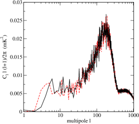
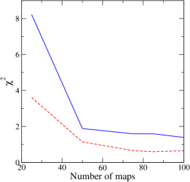
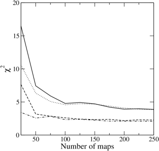
We repeat this procedure to create many Gaussian simulations of the CMB, each being a random Gaussian realisation of the same initial power spectrum. We used different numbers of Gaussian maps in different types of analysis, and we quote each number within the appropriate section. The maps are time-consuming to produce but in each case we check convergence of $\chi^{2}$ (see Figures 3, 12 and 16 for examples). A comparison of the power spectrum of the real and a simulated map can be seen in Figure 1.

Figure 1: The power spectrum of our working maps. WMAP data in the solid line (black in the online version) and one of our Gaussian maps in the dashed line (red in the online version).

Although at small angular scales the noise properties are white, fully understood and easily modelled (see discussion in section 2.1.1), at large angular scales, individual Q, V and W assemblies present noise characteristics which are non-white. Fortunately these are entirely dominated by the signal and one does not need to worry about them (see Fig. 1 of  Hinshaw et al. (2003)). The WMAP team have produced a set of 110 noise maps which include white noise (dominating at small scales), $1/f$ noise (dominating at large scales) and inter-channel correlations for each of the radiometers, and ideally one would like to incorporate all known effects into the analysis. However, being limited by the relatively small number of full noise simulations and due to the high signal to noise ratio at the scales where the noise properties deviate from white, we choose to include only white noise in our Gaussian QVW and single frequency maps.

2.1.3 A more extensive set of masks

In addition to the masks published in the WMAP web-site, a new set of masks was constructed, based on the WMAP team’s kp0 mask which masks the galactic plane plus all known point sources in the sky. The initial motivation came from the need to work with smoothed maps. The QVW maps (real and Gaussian) show a large number of peaks at full resolution which creates a problem concerning the computational time taken to calculate the peak-peak correlation function. So a trade-off between resolution and computational limitations was reached and this consisted of applying an additional Gaussian beam of FWHM = 12 arc minutes to the raw maps (real and Gaussian), as constructed in Section 2.1.1. Because some of the unwanted (masked) signal could leak from the masked regions due to this smoothing, the mask kp0 was also increased (by effectively smoothing it with the same smoothing kernel applied to the data) to create a new mask, dubbed mask 30B. Regions in the smoothed mask with values greater than 0.01 were masked, where the raw mask map has values zero and one, with one meaning masked.

In addition to this extension, the new mask was further modified to include either only the Northern or the Southern hemisphere and also to optionally exclude a region close the galactic plane, $|b|<30^{\circ}$.

A summary of the properties of each of the new masks is given in Table 1.

Table 1: The new and original masks

Mask name	$|b|$ cut	Percentage of removed sky
	(degrees)
kp0	-	23
30B	-	28
30B_knorth	-	64
30B_ksouth	-	64
bcut30_knorth	30	76
bcut30_ksouth	30	77

2.2 Peak-peak correlation function

The two-point correlation function $\xi$ of a discrete distribution of points can be defined as

$$dP=n(1+\xi(\theta))d\Omega$$ (4)

where $dP$ is the probability of finding a data point within a solid angle $d\Omega$, at a distance $\theta$ from another randomly chosen data point and $n$ is the average density of points in the sample. So $\xi(\theta)$ can be seen as an excess of probability of finding a pair at a distance $\theta$, compared to a random catalogue - it is a measurement of clustering - and $\xi(\theta)=0$ indicates a uniform random distribution (no clustering).

There are several estimators suggested in the literature to estimate $\xi(\theta)$ directly from the data. They all work by comparing the sample of points to an uniform, random catalogue with the same spatial distribution as the real data. We used the Hamilton (1993) estimator, which promises fast convergence:

$$\xi(\theta)=\frac{RR(\theta).DD(\theta)}{DR(\theta)^{2}}-1$$ (5)

where $RR(\theta)$ and $DD(\theta)$ are the number of random and data pairs respectively at a distance $\theta$ from each other and $DR(\theta)$ is the number of cross-pairs separated by a distance $\theta$ (all weighted by the number of total random, data and cross pairs in the catalogue). Indeed, we found it to converge faster than the standard estimator, $\xi(\theta)=\frac{DD(\theta)}{DR(\theta)}-1$. We use large random catalogues of 400,000 points for full sky and 200,000 points for single hemispheres, with the same sky cut as the appropriate WMAP map, and ensure that the estimator has converged to a stable value. A hot spot (cold spot) is defined for the purposes of this analysis as the centre of any pixel whose temperature is higher (lower) than the temperature of all pixels with which it shares a boundary.

The correlation function is estimated in 300 equally-spaced bins up to a maximum separation of 1800 arc minutes.

3 Comparison with Gaussian maps

We test the Gaussianity hypothesis of the WMAP data by comparing our estimator of the peak-peak correlation function $\xi(\theta)$ applied to the data with its values when applied to a set of synthetic Gaussian maps with the same cosmology as the WMAP best-fit.

As explained in the previous section, we apply an additional Gaussian beam of FWHM of 12 arc minutes to our real and Gaussian maps, constructed as in section 2.1.1 and 2.1.2, to smooth out some of the small scale noise and make the number of peaks slightly more manageable. We mask all maps with the mask 30B and we select all maxima with temperature above a given threshold $\nu$ and all minima below $-\nu$ ($\nu$ in units of the map rms, $\sigma$). We estimate the peak-peak correlation function using equation (5).

We choose to quantify the robustness of any non-Gaussianity detection by means of the $\chi^{2}$ statistic, which we compute for the WMAP data and for each of the Gaussian maps:

$$\chi^{2}=\sum_{i,j}(\xi_{i}-\bar{\xi}^{G}_{i})C_{ij}^{-1}(\xi_{j}-\bar{\xi}_{j}^{G})$$ (6)

where the covariance matrix $C_{ij}$ is estimated from the Gaussian maps available:

$$C_{ij}=\langle(\xi^{G}_{i,n}-\bar{\xi}^{G}_{i})(\xi^{G}_{j,n}-\bar{\xi}^{G}_{j})\rangle$$ (7)

Here $i,j$ are bins at a given angular separation and the $\bar{\xi}_{i}$ is the average of our estimator over all Gaussian maps of that particular bin. Previously to computing equations (6) and (7) we rebin all data to 19 bins, of which we discard the first one. Rebinning is necessary, otherwise $C_{ij}$ is close to singular and numerically unstable to inversion.

For Gaussian and uncorrelated errors we recall that the $99\%$ confidence level for a reduced $\chi^{2}$ distribution with 18 degrees of freedom comes at $\chi^{2}\leq 0.38$ and $\chi^{2}\geq 1.93$. We also use the $\chi^{2}$ distribution estimated directly from all of the Gaussian maps to give more empirical values for confidence levels - see Section 4.7 for a more detailed discussion on confidence levels. We present our all results using reduced values of $\chi^{2}$ with a total of 18 degrees of freedom.

4 Results

We use the peak-peak correlation function in a number of different ways to investigate the properties of the maps (we use H for Hot, C for Cold, N for North and S for South):

• The most obvious way is to conduct a full-sky analysis in the unmasked regions of the maps, which we do for hot and cold spots separately - $\xi_{H,i}$ and $\xi_{C,i}$.

• We also compute the peak-peak correlation function in each of the hemispheres individually, again looking at hot and cold spots separately in each case - $\xi_{NH,i}$, $\xi_{NC,i}$, $\xi_{SH,i}$ and $\xi_{SC,i}$.

• In addition we look at the difference of correlation between the two hemispheres at a given angular scale and we define $\Delta\xi_{H,i}=\xi_{SH,i}-\xi_{NH,i}$ (similar for cold spots).

• Finally, we take the average of the peak-peak correlation function in the Northern and Southern hemispheres in order to produce a computationally faster way to estimate the full-sky function - $\tilde{\xi}_{H,i}$ (similarly for cold spots).

We explain each of these in detail in the following sections.

4.1 All-sky analysis

We first consider all the hot spots above a certain threshold $\nu\sigma$ (or cold spots below a negative threshold $-\nu\sigma$), for the entire sky except for the masked regions of galactic plane and point sources. The results for a threshold of $\nu=1.5$ are shown in Figure 2. However, with no specific type of non-Gaussianity in mind there is no particular reason to choose any given threshold - too high a threshold reduces the number of peaks and the study is limited by cosmic variance, too low and the computation time is uncomfortably long. Our choice was a compromise to obtain a large number of extrema to get small errors, whilst not being computationally too expensive. We also plot the peak-peak correlation function averaged over 100 Gaussian maps and the error bars on the Gaussian curve are the errors on the mean. The small error bars show good convergence of the average of the peak-peak correlation function from the 100 Gaussian maps. Figure 3 shows the convergence of $\xi_{H}$ and $\xi_{C}$ with increasing number of maps.

Figure 2: The peak-peak correlation function of WMAP’s data hot spots in the dashed (red) line and cold spots in the solid (blue) line. Simulated data (averaged over 100 Gaussian simulations) in the middle (black) line - the error bars shown are the errors on the mean. Note that as these are correlation functions, the errors are correlated.

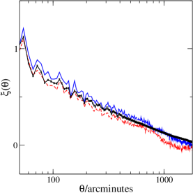
Although not optimally sampled, the structure we see at small angular scales is real structure, as expected from Heavens & Sheth (1999) and Heavens & Gupta (2001)

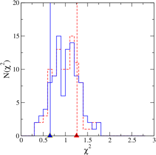
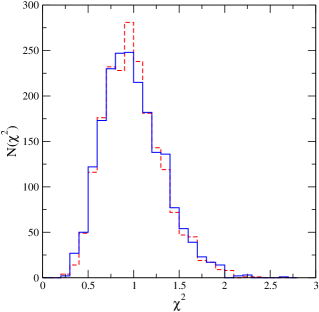
We see immediately that neither the hot spots nor the cold spots follow the Gaussian simulations - the cold spots show an excess of correlation whereas the hot spots show a lack of correlation with respect to the Gaussian simulations. These differences are, however, not significant; one disadvantage of the correlation function is that the errors can be highly correlated. The distribution of the $\chi^{2}$ values for all of the Gaussian maps can be seen in Figure 4, together with the values for the WMAP data. We find $\chi^{2}=1.25$ for the hot spots and $\chi^{2}=0.65$ for the cold spots, which are within the Gaussian $1\sigma$ confidence level. So the maps analysed in this way do not show any sign of non-Gaussianity. This is in agreement with Larson & Wandelt (2005) who also find no significant deviation from Gaussianity when they compute the peak-peak correlation of hot and cold spots (although they work with lower resolution maps).

Figure 3: Convergence of $\xi_{C}$ (solid, blue line) and $\xi_{H}$ (dashed, red line) with number of Gaussian maps used to estimate $\bar{\xi}^{G}_{i}$ and $C_{ij}$ as defined in Section 3.

Figure 4: The distribution of reduced $\chi^{2}$ values for all of the 100 Gaussian maps: hot spots in the dashed (red) line and cold spots in the solid (blue) line. The $\chi^{2}$ values for the WMAP data are represented by the small triangles and vertical lines.

There have been numerous claims in the literature (see Introduction) that the WMAP maps show an asymmetry in their statistical properties between the Northern and the Southern hemispheres, so we turn to this next.

4.2 North-South analysis

To further investigate any discrepancy between the WMAP data and our Gaussian simulations we apply the masks 30BN and 30BS to all our maps and proceed to get an estimation of the peak-peak correlation function for the Northern and Southern hemispheres separately.

Figure 5 shows the peak-peak correlation function of the WMAP data for cold and hot spots calculated in the Northern and Southern hemispheres.

Figure 5: The peak-peak correlation for the WMAP data in the two hemispheres - solid lines show the South and dashed lines the North. The inner pale (red) lines show hot spots and the outter (blue) lines show cold spots.

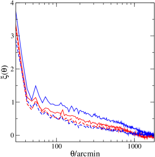
We find a difference between the correlation of cold spots in the different hemispheres. Again we use a $\chi^{2}$ statistic, $\chi^{2}_{NS}$ for $\Delta\xi_{C}$ and $\Delta\xi_{H}$, with the mean and covariance matrix estimated from 250 Gaussian maps. By analysing each hemisphere seperately, we are reducing the number of peaks available for the estimation of the peak-peak correlation function. Hence we found that a greater number of maps was needed to ensure good convergence of the average peak-peak correlation function and of the covariance matrix. See Figure 12 in the next section for convergence of some of the statistics with increasing number of maps.

We calculate $\chi^{2}_{NS}$ for our ensemble of Gaussian maps, whose distribution can be seen in Figure 6, together with the $\chi^{2}_{NS}$ value calculated for the WMAP data, for hot and cold spots.

Figure 6: The distribution of reduced $\chi^{2}_{NS}$ for all 250 Gaussian maps. Hot spots in the dashed (red) line and cold spots in the solid (blue) line. The $\chi^{2}_{NS}$ values for the WMAP data are represented by the small triangles and vertical lines.

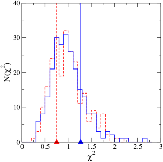
We note that the fact we are finding the South-North difference not to be significant ($\chi^{2}_{NS}=0.748$ and $1.27$ for hot and cold spots respectively) may be due to the fact that the peak-peak correlation function of threshold-selected peaks is highly sensitive to cosmic variance in the low multipoles. All the estimators are highly correlated and are shifted up and down in synchrony from Gaussian realisation to Gaussian realisation: the noisy low-$\ell$ multipoles can shift large numbers of peaks above or below the threshold depending on the mode amplitude. This suggests that the use of a high-pass filter - effectively removing the signal from cosmic variance above a given angular scale on the sky - may be an efficient way to increase the sensitivity to non-Gaussian features.

4.3 Constraining in harmonic space

We high-pass filter our maps (real and Gaussian) by constructing several window functions given by ${\mathcal{W}}_{\ell_{cut}}(\ell)=0$ for $\ell\leq\ell_{cut}$, ${\mathcal{W}}_{\ell_{cut}}(\ell)=1$ otherwise, which we apply to our maps and we investigate cases with $\ell_{cut}=0,5,10,15,20,25,30$ and $40$.

We mask the WMAP maps before filtering. This is necessary because of the presence of foregrounds - the strong ringing effect in pixel space which results from such a sharp cut-off in harmonic space causes unwanted foreground signal to leak from the masked region. We follow the algorithm described below:

• We mask the WMAP data.

• We extract the $a_{lm}$ coefficients using HEALPix’s routine anafast.

• We multiply the harmonic coefficients by the respective window function.

• We generate the map in pixel space by using the HEALPix’s routine synfast.

• We re-mask the map.

• We remove the monopole/dipole from the unmasked regions.

Since there is no foreground contamination in the Gaussian maps, there is no need to apply the initial mask. For testing purposes, we applied both methods to a number of Gaussian maps and found them to produce the same final results.

For each case we construct an ensemble of 250 Gaussian maps. We compute $\Delta\xi_{H}$, $\Delta\xi_{C}$, $\xi_{NH}$, $\xi_{NC}$, $\xi_{SH}$, $\xi_{SC}$, $\tilde{\xi}_{H}$ and $\tilde{\xi}_{C}$ for all our Gaussian maps as well as the WMAP data. Figure 12 shows convergence of $\xi_{SC}$ and $\Delta\xi_{C}$ with number of maps in the solid and dashed lines respectively. The same plot also shows the convergence of the same statistics but this time calculated in a single-frequency Q-band map (see Section 4.5 for a single-frequency analysis). We quote all significance levels in Table 2.

Figure 7: $\Delta\xi_{C}(\theta)$ for the WMAP map high-pass filtered with different values of $\ell_{cut}$.

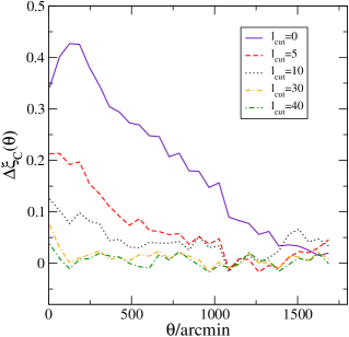
Figure 7 shows $\Delta\xi_{C}(\theta)$ for some different $\ell_{cut}$ in the WMAP data. We note that the difference between the Southern and Northern hemispheres decreases as we remove more and more of the low order multipoles. This could be either due to the fact that cosmic variance alone is to blame for the North/South difference we see, or it could be due to the fact that whatever is causing this North/South difference is intrinsically a large scale effect.

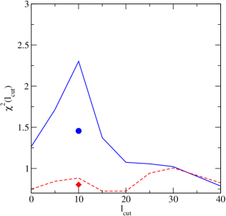
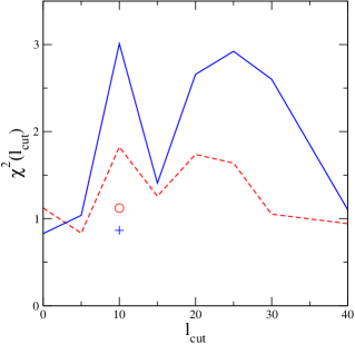
We test the significance of each of these differences by using $\chi^{2}_{NS}$. Figure 8 shows $\chi_{NS}^{2}(\ell_{cut})$ for cold and hot spots. We plot the distribution of $\chi^{2}_{NS}$ using all the different $\ell_{cut}$ Gaussian maps - these maps are not strictly independent (although the statistics share the same underlying $\chi^{2}$ distribution over all values of $\ell_{cut}$) so we use only the 250 independent maps at each $\ell_{cut}$ to draw conclusions about the significance of each detection - see Section 4.7. The added histogram over the 2000 maps can be seen in Figure 9.

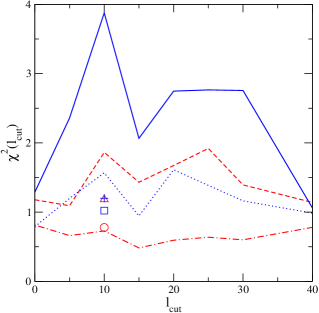
We do the same test and construct identical plots for all our statistics: $\tilde{\xi}_{H}$/$\tilde{\xi}_{C}$ in Figure 10 and $\xi_{NH}$/$\xi_{NC}$/$\xi_{SH}$/$\xi_{SC}$ in Figure 11. The added histograms across all values of $\ell_{cut}$ for these statistics are very similar to that shown in Figure 9.

The first point to make is that the non-Gaussianity is consistently absent at $\ell_{cut}=40$: there is no evidence from the peak-peak correlation function of non-Gaussianity on scales with $\ell>40$.

The most significant non-Gaussian detections come from the cold spots in the Southern hemisphere, $\xi_{SC}$, at $\ell_{cut}=10$ (with a value of $\chi^{2}=3.877$ and a probability formally estimated to be $10^{-7}$ - see Section 4.7), where we also find significant detections in the South-North difference for cold spots, $\Delta\xi_{C}$ $(\chi^{2}_{NS}=2.302)$, and in the average of Northern and Southern hemispheres for cold spots, $\tilde{\xi}_{C}$ $(\chi^{2}=3.011)$. In addition to this, we have less significant detections at $\ell_{cut}=20,25$ and $30$ in $\xi_{SC}$ ($\chi^{2}=2.747,2.764$ and $2.756$ respectively) and $\tilde{\xi}_{C}$ ($\chi^{2}=2.658,2.923$ and $2.601$, see Figures 10 and 11). All of these do not appear in a North minus South analysis. This could be simply because the signal is not significant enough to show up in such analysis (we are roughly doubling the variance of our estimator by subtracing the data of the Sorthern and Northern hemispheres).

Figure 8: $\chi^{2}_{NS}$ as a function of $\ell_{cut}$ for the WMAP data. Hot spots in the solid (red) line, cold spots in the dashed line (blue). The circle (blue) and the diamond (red) are the $\chi^{2}$ value (cold spots and hot spots respectively) for runs with the regions of sky within $30$ degrees of the galactic plane removed (see Section 4.4). We recall that the 99$\%$ confidence levels for a $\chi^{2}$ distribution of 18 degrees of freedom come at $\chi^{2}\leq 0.42$ and $\chi^{2}\geq 1.93$. See Figure 9 for the distribution of the $\chi^{2}_{NS}$ values of all Gaussian maps.

Figure 9: The added distribution of $\chi_{NS}^{2}$ values for all our Gaussian maps at all different $\ell_{cut}$. Hot spots in the dashed (red) line, cold spots in the solid (blue) line. Similar histograms were produced for all of our other statistics, and all show an identical added distribution of reduced $\chi^{2}$ values.

Figure 10: $\chi^{2}(\ell_{cut})$ for $\tilde{\xi}_{C}$ solid (blue) line and $\tilde{\xi}_{C}$ dashed (red) line for the WMAP data. The single points at $\ell_{cut}=10$ are the $\chi^{2}$ values for cold spots (blue cross) and hot spots (red circle) in runs with the regions of sky within $30$ degrees of the galactic plane removed (see Section 4.4).

Figure 11: $\chi^{2}(\ell_{cut})$ for $\xi_{NC}$ (blue dotted line), $\xi_{NH}$ (red dot-dashed line), $\xi_{SC}$ (blue solid line) and $\xi_{SH}$ (red dashed line) for the WMAP data. The single point at $\ell_{cut}=10$ are the $\chi^{2}$ values for runs with the regions of sky within $30$ degrees of the galactic plane removed (see Section 4.4): $\xi_{NH}$ in the red circle, $\xi_{NC}$ in the blue square, $\xi_{SH}$ in the red triangle and $\xi_{SC}$ in the blue cross.

Figure 12: Convergence of some of our statistics which yielded detections of non-Gaussianity with increasing number of maps. For the QVW map we show $\xi_{SC}$ in the solid line and $\Delta\xi_{C}$ in the dashed line. For the single-frequency Q-band map we show $\xi_{SC}$ in the dotted line and $\Delta\xi_{C}$ in the dot-dashed line

4.4 Constraining in real space

We further investigate the origin of this detection by removing extra regions near the masked galactic plane. We work on the maps where the significance of the signal is the strongest (those with $\ell_{cut}=10$), which we mask with the extended masks: bcut30_knorth and bcut30_ksouth.

We proceed the same way as before and compute the full set of estimators: $\Delta\xi_{H}$, $\Delta\xi_{C}$, $\xi_{NH}$, $\xi_{NC}$, $\xi_{SH}$, $\xi_{SC}$, $\tilde{\xi}_{H}$ and $\tilde{\xi}_{C}$ for all our Gaussian maps as well as the WMAP data and use the adequate $\chi^{2}$ statistic for each of them to test the WMAP data for non-Gaussianity (we generate new random catalogues whose spacial distribution follows that of the new masks).

Figures 8, 10 and 11 show how the new $\chi^{2}$ values compare with the ones previously obtained when we did not use any extra galactic cut - all values drop significantly to values which are perfectly consistent with the Gaussian hypothesis (the most extreme value being $\chi^{2}_{NS}=1.46$ for $\Delta\xi_{C}$) , indicating that our significant non-Gaussian detection in the cold spots is located within $30$ degrees of the galactic plane. Clearly, this hints at residual foreground contamination associated with the Milky Way.

We note that we have only tested this on maps with $\ell_{cut}=10$ since this is where we have found our strongest detection. We cannot discard the possibility that the effect that yields detections on maps with $\ell_{cut}=15,25$ and $30$ is a different effect altogether which does not lie in the galactic region.

4.5 A single-frequency analysis

To check whether the non-Gaussian signal we detect is related to possible residual foregrounds in the WMAP data we conduct a single frequency analysis of the maps. Indeed, the expected galactic foreground contribution to the WMAP maps consists mainly of synchrotron, free-free and dust emission. All of these effects are frequency-dependent and obviously non-Gaussian. If any foreground residuals are still present in the foreground-cleaned data then we would expect them to contribute differently to each of the different frequency maps. We note that any residual noise may also contribute differently to each frequency.

We construct the real map and each of the 250 simulated single frequency maps by following the same method we used to construct the co-added QVW map (described in Section 2.1), but we use only the relevant DAs for each of the frequencies. We then smooth the WMAP and Gaussian maps with a 12 arc minute FWHM Gaussian beam and high-pass filter with a $\ell_{cut}=10$ window function (where we had the most significant non-Gaussian detection).

We calculate the full set of estimators for each of the frequencies: $\Delta\xi_{H}$, $\Delta\xi_{C}$, $\xi_{NH}$, $\xi_{NC}$, $\xi_{SH}$, $\xi_{SC}$, $\tilde{\xi}_{H}$ and $\tilde{\xi}_{C}$, for which the $\chi^{2}$ values can be seen in Figures 13, 14 and 15.

Figure 13: $\chi^{2}_{NS}$ for all three frequencies: Q (41 GHz), V (61 GHz) and W (94 GHz) on maps with $\ell_{cut}=10$. Statistics for cold spots in the solid (blue) line, for hot spots in the dashed (red) line.

Figure 14: $\chi^{2}$ for all three frequencies: Q (41 GHz), V (61 GHz) and W (94 GHz) on maps with $\ell_{cut}=10$. Statistics for $\xi_{NH}$ in the dot dashed (red) line, $\xi_{NC}$ in the dotted (blue) line, $\xi_{SH}$ in the dashed (red) line and finally for $\xi_{SC}$ in the solid (blue) line.

Figure 15: $\chi^{2}$ for all three frequencies: Q (41 GHz), V (61 GHz) and W (94 GHz) on maps with $\ell_{cut}=10$. Statistics for $\tilde{\xi}_{H}$ in the dashed (red) line and for $\tilde{\xi}_{C}$ in the solid (blue) line.

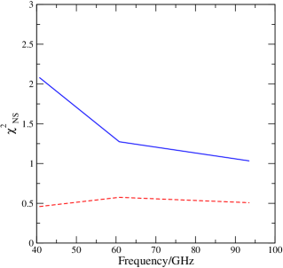
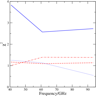
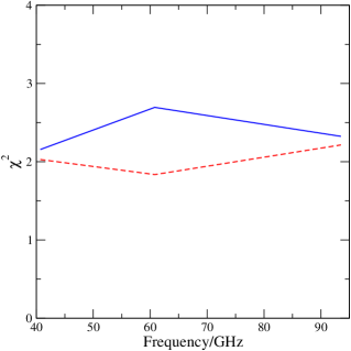
We find significant non-Gaussian signals coming from the cold spots $\Delta\xi_{C}$ in the Q band ($\chi^{2}_{NS}=2.081$) and $\xi_{SC}$ in all three bands, although it is strongest in the Q band (with $\chi^{2}=3.831$). We also find detections in our full-sky estimates in the cold spots in all three bands, and, for the first time, in the hot spots in bands Q and W (see Figure 15).

We may be seeing a frequency-dependent type of non-Gaussianity, although we can not put aside the possibility of a cosmological origin. To improve readability we do not present the plots with the $\chi^{2}$ distributions of the 250 Gaussian maps for each of the frequencies and for each of the estimators. We do, however, quote the number of Gaussian maps with a $\chi^{2}_{Gaussian}\geq\chi^{2}_{WMAP}$ for all significant detections in Table 2, Section 4.7.

4.6 Removing the cosmological signal

In order to investigate the possibility of any contributions from foregrounds or unexplained noise properties, we remove what is taken to be the cosmological signal from our analysis.

To do so we subtract different single-frequency maps to produce three maps which contain only a mix of subtracted residual foregrounds (if any) and noise. We produce a $V-Q$, a $V-W$ and a $Q-W$ map, which are simply a pixel-by-pixel subtraction of each of the single frequency maps, constructed as described in Section 4.5.

With the cosmological signal removed, the detailed noise properties of these 3 subtracted maps at large angular scales now become important for our analysis and one should be careful when constructing equivalent Gaussian maps (see Section 2.1.2). We therefore take a slightly different route to construct the Gaussian simulations with which we compare the WMAP data, and we now make use of the 110 noise simulations supplied by the WMAP team. We construct single-frequency noise maps by adding the respective individual radiometer simulations following the same weighting scheme as described in Section 2.1, which we then smooth and high-pass filter with a $\ell_{cut}=10$ window. We then subtract different frequency noise maps in order to produce 110 simulations with which we compare our real $V-Q$, $V-W$ and $Q-W$ maps. We reemphasize that for maps which include the signal, the non-white nature of the noise at low-$\ell$ is essentially irrelevant, as the signal dominates entirely  (Hinshaw et al., 2003).

We construct $\Delta\xi_{H}$, $\Delta\xi_{C}$, $\xi_{NH}$, $\xi_{NC}$, $\xi_{SH}$, $\xi_{SC}$, $\tilde{\xi}_{H}$ and $\tilde{\xi}_{C}$ for the simulations and the real data as before and use the respective $\chi^{2}$ statistic to probe for non-Gaussian signatures.

In this case, our total number of maps was constrained by the number of noise simulations provided by the WMAP team. Figure 16 shows how the reduced $\chi^{2}$ values for $\Delta\xi_{H}$, $\Delta\xi_{C}$, $\xi_{NH}$, $\xi_{NC}$, $\xi_{SH}$ and $\xi_{SC}$ in the $Q-W$ map change with number of simulated maps used (the $Q-V$ and $V-W$ maps produced very similar results). The results show clear convergence to some value well within the $1\sigma$ confidence levels. The reason why we observe faster convergence in these maps could simply be due to the fact that we are removing the cosmological signal from the analysis and with it much of the variance.

Figure 16: Convergence of the reduced $\chi^{2}$ values for $\Delta\xi_{H}$, $\Delta\xi_{C}$, $\xi_{NH}$, $\xi_{NC}$, $\xi_{SH}$ and $\xi_{SC}$ in the $Q-W$ map as a function of number of Gaussian maps.

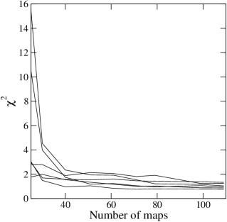
Figure 17 shows $\xi_{NC}$ and $\xi_{SC}$ for the WMAP data and also $\bar{\xi}^{G}_{NC}$ and $\bar{\xi}^{G}_{SC}$ where the average is done over the 110 simulated $V-Q$ noise maps.

Figure 17: $\xi_{NC}$ and $\xi_{SC}$ estimated from the $V-Q$ subtracted maps. WMAP’s data are the solid line for Southern hemisphere and dashed line for Northern hemisphere (both in blue). Gaussian averaged data in dotted line for Southern hemisphere, dot dashed line for Northern hemisphere (both in black).

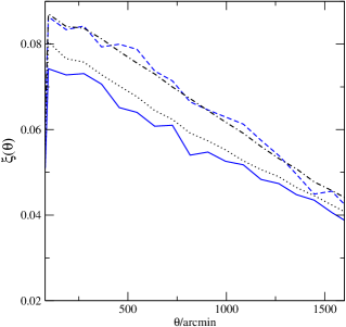
Some comments on this figure are appropriate. Firstly we note that there is an intrinsic North/South asymmetry in the Gaussian noise maps. This is due to the large-scale structure generated in the noise due to the uneven scanning pattern of the WMAP satellite. We recall that pixel noise is weighted according to the number of times a pixel has been observed, and as such this feature is fully simulated in all our previous maps. This large-scale structure combined with the fact we are applying an asymmetric mask to the data results in the non-zero and North/South asymmetric peak-peak correlation function we see. We draw attention to the fact that this asymmetry is qualitatively different from what we found in Sections 4.2, 4.3, 4.4 and 4.5, since we now find an excess in correlation in the Northern hemisphere, as opposed to in the South. This excess in correlation in the North is indeed seen in the Gaussian-averaged peak-peak correlation function of all our previous maps, although on a much smaller scale. Finally we note that there is a more noticeable deviation of the WMAP data from the Gaussian simulations in the Southern hemisphere. However, we find none of these to be significant. In fact, this statement extends to the other two cases: $V-W$ and $Q-W$. We find no signs of non-Gaussianity in any of the estimators in any of our combined noise and foreground maps, with all the $\chi^{2}$ values well within values which are consistent with the Gaussian hypothesis (our most extreme $\chi^{2}$ value comes from $\xi_{SH}$ in the $V-Q$ map, where we find $\chi^{2}=1.49$ - see Table 2 in the next section for a summary of the most extreme values in all three maps).

4.7 A summary of our results

In this subsection we take the opportunity to summarise our results into one table and to elaborate on the confidence levels we have quoted throughout the paper. We do this by presenting a table with all the statistics for which we have found the WMAP data to have a reduced $\chi_{WMAP}^{2}\geq 2$, Table 2.

We recall that in all cases we have rebinned the data into 19 linearly-spaced bins, of which we use the last 18 to compute each of the $\chi^{2}$ statistics. The $P_{theory}$ column gives the probability of randomly obtaining a given value of $\chi^{2}\geq\chi^{2}_{WMAP}$ assuming the underlying distribution is a $\chi^{2}$ distribution with 18 degrees of freedom, and the $N_{Gaussian}$ column shows how many Gaussian maps have a $\chi^{2}\geq\chi^{2}_{WMAP}$ for the correspondent estimator (the number in brackets in the total number of Gaussian maps). It is worth noting that the $\chi^{2}$ distribution we estimate from the Gaussian maps fits a $\chi^{2}$ distribution with 18 degrees of freedom which has been shifted slightly by $\Delta\chi^{2}\approx 0.1$ to lower values. Hence any limit on high values of $\chi^{2}$ based on this theoretical distribution is a conservative one. These are the limits we quote throughout the text. Shifting the Gaussian $\chi^{2}$ distribution by $\Delta\chi^{2}=0.1$ results in the $P_{theory}$ values in Table 2 roughly being halved.

We draw attention to our most striking detections, which come from the cold spots in the Southern hemisphere, appearing both in the co-added QVW map and in the single frequency Q band map with reduced $\chi^{2}$ values of $3.877$ and $3.831$ respectively.

Table 2: Our main detections. We present all situations which yielded vales of $\chi^{2}\geq 2$. In addition to this and for the sake of completeness we also present the most extreme $\chi^{2}$ values obtained in Section 4.6. $P_{theory}$ is the theoretical probability of randomly obtaining a reduced $\chi^{2}\geq\chi^{2}_{WMAP}$ assuming a reduced $\chi^{2}$ distribution with 18 degrees of freedom and $N_{Gaussian}$ is the total number of Gaussian maps with $\chi^{2}\geq\chi^{2}_{WMAP}$. In brackets is the number of Gaussian realisations used for each statistic.

Map	$\ell_{cut}$	Estimator	$\chi^{2}_{WMAP}$	$P_{theory}$	$N_{Gaussian}$
QVW	10	$\Delta\xi_{C}$	2.302	$1.32\times 10^{-3}$	0 (250)
QVW	5	$\xi_{SC}$	2.358	$9.58\times 10^{-4}$	0 (250)
QVW	10	$\xi_{SC}$	3.877	$4.91\times 10^{-8}$	0 (250)
QVW	20	$\xi_{SC}$	2.747	$9.15\times 10^{-5}$	0 (250)
QVW	25	$\xi_{SC}$	2.764	$8.23\times 10^{-5}$	0 (250)
QVW	30	$\xi_{SC}$	2.756	$8.65\times 10^{-5}$	0 (250)
QVW	10	$\tilde{\xi}_{C}$	3.011	$1.71\times 10^{-5}$	0 (250)
QVW	20	$\tilde{\xi}_{C}$	2.658	$1.59\times 10^{-4}$	0 (250)
QVW	25	$\tilde{\xi}_{C}$	2.923	$3.01\times 10^{-5}$	0 (250)
QVW	30	$\tilde{\xi}_{C}$	2.601	$2.25\times 10^{-4}$	0 (220)
Q	10	$\Delta\xi_{C}$	2.081	$4.57\times 10^{-3}$	2 (250)
Q	10	$\xi_{SC}$	3.831	$6.78\times 10^{-8}$	0 (250)
V	10	$\xi_{SC}$	2.571	$2.70\times 10^{-4}$	0 (250)
W	10	$\xi_{SC}$	2.729	$1.02\times 10^{-4}$	0 (250)
Q	10	$\tilde{\xi}_{C}$	2.156	$3.02\times 10^{-3}$	0 (250)
V	10	$\tilde{\xi}_{C}$	2.695	$1.26\times 10^{-4}$	0 (250)
W	10	$\tilde{\xi}_{C}$	2.325	$1.16\times 10^{-3}$	0 (250)
Q	10	$\tilde{\xi}_{H}$	2.029	$6.04\times 10^{-3}$	0 (250)
W	10	$\tilde{\xi}_{H}$	2.215	$2.17\times 10^{-3}$	1 (250)
V-Q	10	$\xi_{SH}$	1.494	$8.10\times 10^{-2}$	10 (110)
Q-W	10	$\Delta\xi_{H}$	1.328	$1.58\times 10^{-1}$	22 (110)
V-W	10	$\Delta\xi_{C}$	1.426	$1.07\times 10^{-2}$	10 (110)

5 Conclusions

In this paper we have used the peak-peak correlation function of the local extrema in the CMB temperature fluctuations to probe for non-Gaussian signatures. As explained at the start of Section 4, we have constructed a series of statistics which look both at cold and hot spots in the full sky, in the Northern and Southern hemispheres separately and at the difference between both hemispheres. We have also looked at a variety of maps: a co-added QVW map with a standard mask applied, a co-added QVW map with an extended galactic cut applied, three co-added maps at the same frequency and three differences maps so as to remove the cosmological signal. In the case of the co-added QVW map we also investigated eight different cases with some of the low multipoles removed.

Our main results are summarised in Table 2 in Section 4.7 - we find strong evidence for non-Gaussianity, mainly associated with the cold spots and with the Southern hemisphere; this non-Gaussianity disappears completely if we filter out the harmonic modes $\ell\leq 40$ and at least partially if we exclude sky within $|b|<30^{\circ}$, so it is a large-scale effect associated with the galactic plane.

Recently, Larson & Wandelt (2005) have also used the peak-peak correlation function of cold and hot spots in their search for non-Gaussianity. Direct comparison of results is not straightforward as the resolutions of the maps used in the two studies are significantly different. However, in the simplest case where both groups looked at the full sky CMB temperature field (with equivalent masks based on the standard kp0 mask applied), both results are in agreement in the sense that both fail to yield a detection. We believe this lack of detection is a result of large cosmic variance in low-$\ell$ multipoles.

We investigate this further by removing some of the low order multipoles from the maps, in the hope that by doing so we are increasing our sensitivity to non-Gaussian features by reducing the effects of cosmic variance. Once we remove all harmonic modes with $\ell\leq 10$ we systematically find anomalies related to the cold spots in the WMAP data and, when looking at both hemispheres separately, we not only find a striking North/South asymmetry, we repeatedly find the strongest anomalies to be in the Southern hemisphere. This is not unheard of: Vielva et al. (2004) first found an anomalous large cold spot in the Southern hemisphere (nicknamed The Spot), detection which was followed by Cruz et al. (2005), Mukherjee & Wang (2004) and McEwen et al. (2005) and confirmed repeatedly. However, we do find that our detections disappear when we exclude sky regions within 30 degrees of the galactic place (we recall that The Spot is localised at approximately $(b=-57^{\circ},l=209^{\circ})$, well outside our cut regions of sky). We therefore conclude that our detections come mainly from something other than The Spot.

The North/South asymmetry is also something which has been quoted time and time again in the literature: Park (2004), Eriksen et al. (2004a, b, 2005) and other work previously quoted in this paper have consistently found non-Gaussian asymmetries between the two galactic hemispheres. The asymmetry we find in this study seems to be a large scale effect, once again related only to the cold spots and to be contained within 30 degrees of the galactic plane.

We investigate our detections further by firstly conducting an analysis in single frequency maps. We find some evidence for a dependence of the signal with frequency when we look at different hemispheres (peaking at 41GHz, corresponding to the Q band and in agreement with Liu & Zhang (2005)), but this detection does not appear in a full-sky analysis. Secondly we remove the cosmological signal from the analysis by subtracting different frequency maps and testing the resulting foreground/noise combination maps for non-Gaussian signals. We find no signs of non-Gaussianity in these subtracted maps.

How do we make sense of these results? A simple explanation seems untenable. The fact that the signal becomes insignificant when the galactic plane is removed suggests unsubtracted galactic foregrounds are responsible; the large-scale nature of the signal is certainly consistent with this picture. One would then expect the individual frequency maps to show a significant signal, and this we do find, most strikingly in the Q band. However, the difference maps do not show a significant detection; these maps should directly test the residual foregrounds and noise, so the absence of detected non-Gaussianity does not obviously support this picture. We can reconcile these observations if the residual foregrounds affect more than one frequency band, and the subtraction removes the contamination to some extent. The fact that we find non-Gaussianity in all the single-frequency bands adds some support to this complex picture. In our view this is the most likely explanation for the results we find, but we cannot exclude a primordial origin for at least part of the non-Gaussian signal.

6 Acknowledgments

RT is funded by the Fundação para a Ciência e a Tecnologia under the reference PRAXIS SFRH/BD/16973/04. PGC is supported by the PPARC through a Postoctoral Rolling grant. SG is supported by the PPARC. SG and RT would like to thank Rob Crittenden for helpful discussions. RT would like to thank John Peacock for helpful discussions and suggestions. We acknowledge the use of the Legacy Archive for Microwave Background data analysis (LAMBDA). Support for LAMBDA is provided by the NASA Office of Space Science. Some of the results in this paper have been derived using the HEALPix (Górski, Hivon, and Wandelt 1999) package.

References

- Aghanim et al. (2003) Aghanim N., Kunz M., Castro P.G., Forni O., 2003, A&A, 406, 797
- Banday, Zaroubi & Górski (2000) Banday A.J., Zaroubi S., Górski K.M., 2000, ApJ, 533, 575
- Bennett et al. (2003) Bennett C.L. et al., 2003, ApJS, 148, 1
- Berera & Heavens (2000) Berera A., Heavens A.F., 2000, Phys. Rev. D62, 123513
- Berera, Fang & Hinshaw (1998) Berera A., Fang F.-Z., Hinshaw G., 1998, Phys. Rev. D57, 2207
- Blanchard & Schneider (1987) Blanchard A., Schneider J., 1987, A&A, 184, 1
- Castro (2003) Castro P.G., 2003, Phys. Rev. D67, 123001
- Coles et al. (2004) Coles P. et al., 2004, MNRAS, 350, 983
- Colley & Gott (2003) Colley W.N., Gott J.R., 2003 MNRAS, 344, 686
- Cooray (2001a) Cooray A., 2001a, Phys. Rev. D64, 043516
- Cooray (2001b) Cooray A., 2001b, Phys. Rev. D64, 063514
- Cooray & Kesden (2003) Cooray A., Kesden M., 2003, New Astronomy, 8, 255
- Cooray & Hu (2000) Cooray A., Hu W., 2000, ApJ, 534, 533
- Copi, Huterer & Starkman (2004) Copi C.J., Huterer D., Starkman G.D, 2004, Phys. Rev. D70, 043515
- Cruz et al. (2005) Cruz M. et al., 2005, MNRAS, 356, 29
- Efstathiou (2003) Efstathiou G., 2003, MNRAS, 343, 95
- Eriksen et al. (2004a) Eriksen H.K. et al., 2004a, ApJ, 605, 14
- Eriksen et al. (2004b) Eriksen H.K. et al., 2004b, ApJ, 612, 633
- Eriksen et al. (2005) Eriksen H.K. et al., 2005, ApJ, 622, 58
- Ferreira, Magueijo & Górski (1998) Ferreira P.G., Magueijo J., Górski K.M., 1998, ApJ, 503, L1
- Guth (1981) Guth A., 1981, Phys. Rev. D23, 347
- Gurzadyan et al. (2005) Gurzadyan V.G. et al., 2005, Mod.Phys.Lett., A20, 813
- Hamilton (1993) Hamilton A.J., 1993, ApJ, 417, 19
- Heavens (1998) Heavens A.F., 1998, MNRAS, 299, 805
- Heavens & Gupta (2001) Heavens A.F., Gupta S., 2001, MNRAS, 324, 960
- Heavens & Sheth (1999) Heavens A.F., Sheth R.K., 1999, MNRAS, 310, 1062
- Hinshaw et al. (2003) Hinshaw G. et al., 2003, ApJS, 148, 135
- Hu (2001) Hu W., 2001, Phys. Rev. D64, 083005
- Jaffe et al. (2005) Jaffe T.R., et al., 2005, preprint (astro-ph/0503213)
- Jungman et al. (1996) Jungman G., Kamionkowski M., Kosowsky A., Spergel D., 1996 Phys. Rev. D54, 1332
- Komatsu (2001) Komatsu E., 2002, Ph.D. thesis, Tohoku University
- Komatsu et al. (2003) Komatsu E. et al., 2003, ApJS, 148, 119
- Land & Magueijo (2005a) Land K., Magueijo J., 2005a, MNRAS, 2005, 357, 994
- Land & Magueijo (2005b) Land K., Magueijo J., 2005b, preprint (astro-ph/0502237)
- Land & Magueijo (2005c) Land K., Magueijo J., 2005c, preprint (astro-ph/0502574)
- Larson & Wandelt (2005) Larson D.L., Wandelt B.D., 2005, preprint (astro-ph/0505046)
- Liu & Zhang (2005) Liu X. and Zhang, S.N., 2005, preprint (astro-ph/0504589)
- Magueijo (2000) Magueijo J., 2000, ApJL, 528, 57
- Magueijo & Medeiro (2004) Magueijo J., Medeiros J., 2004, MNRAS, 351, L1
- McEwen et al. (2005) McEwen J.D. et al., 2005, MNRAS, 359, 1583
- Mukherjee & Wang (2004) Mukherjee P., Wang Y., 2004, ApJ, 613, 51
- Ostriker & Vishniac (1986) Ostriker J.P., Vishniac E.T., 1986, ApJ, 306, L51
- Park (2004) Park C.-G., 2004, MNRAS, 349, 313
- Rees & Sciama (1968) Rees M.J, Sciama D.W., 1968, Nat517, 611
- Smoot et al. (1992) Smoot G. et al., 1992, ApJ, 396, L1
- Sunyaev & Zeldovich (1972) Sunyaev R., Zel’dovich Y., 1972, Comm. Astrophys. Sp. Phys., 4, 173
- Tegmark, Oliveira-Costa & Hamilton (2003) Tegmark M., Oliveira-Costa A., Hamilton A., 2003, Phys. Rev. D68, 123523
- Verde & Spergel (2002) Verde L., Spergel D.N., 2002, Phys. Rev. D65, 3007
- Vielva et al. (2004) Vielva P. et al., 2004, ApJ, 609, 22
- Wandelt, Hivon & Górsky (2001) Wandelt B.D., Hivon E., Górski K.M., 2001, Phys. Rev. D64, 083003