Numerical Relativistic Hydrodynamics Based on the Total Variation Diminishing Scheme

Abstract

This paper describes a multidimensional hydrodynamic code which can be used for studies of relativistic astrophysical flows. The code solves the special relativistic hydrodynamic equations as a hyperbolic system of conservation laws based on the total variation diminishing (TVD) scheme. It uses a new set of conserved quantities and employs an analytic formula for transformation from the conserved quantities in the reference frame to the physical quantities in the local rest frame. Several standard tests, including relativistic shock tubes, a relativistic wall shock, and a relativistic blast wave, are presented to demonstrate that the code captures discontinuities correctly and sharply in ultrarelativistic regimes. The robustness and flexibility of the code are demonstrated through test simulations of the relativistic Hawley-Zabusky shock and a relativistic extragalactic jet.

1 Introduction

Many high-energy astrophysical problems involve relativistic flows, and thus understanding relativistic flows is important for correctly interpreting astrophysical phenomena. For instance, intrinsic beam velocities larger than $0.9c$ are typically required to explain the apparent superluminal motions observed in relativistic jets in microquasars in the Galaxy (Mirabel & Rodríguez, 1999) as well as in extragalactic radio sources associated with active galactic nuclei (Zensus, 1997). In some powerful extragalactic radio sources, ejections from galactic nuclei produce true beam velocities of more than $0.98c$. Relativistic descriptions are also inevitable in other situations of rapid expansion such as the early stages of supernova explosions (Burrows, 2000) and the production of energetic gamma-ray bursts (Mészáros, 2002). In the general fireball model of gamma-ray bursts, the internal energy of gas is converted into the bulk kinetic energy during expansion and this expansion leads to relativistic outflows with high bulk Lorentz factors $\gtrsim 100$. Since such relativistic flows are highly nonlinear and intrinsically complex, in addition to possessing large Lorentz factors, often studying them numerically is the only possible approach.

For numerical study of non-relativistic hydrodynamics, explicit finite difference upwind schemes have been developed and implemented successfully. The schemes which have been used for astrophysical researches include the Roe scheme (Roe, 1981), the total variation diminishing (TVD) scheme (Harten, 1983), the piecewise parabolic method (PPM) scheme (Colella & Woodward, 1984), and the essentially non-oscillatory (ENO) scheme (Harten et al., 1987). These schemes are based on exact or approximate Riemann solvers using the characteristic decomposition of the hyperbolic system of hydrodynamic conservation equations. They all are able to capture sharp discontinuities robustly in the complex flows, and to describe the physical solution accurately.

Although the upwind schemes were originally developed for non-relativistic hydrodynamics, some have been extended to special relativistic hydrodynamics. For instance, Dolezal & Wong (1995) adapted the ENO scheme to one-dimensional relativistic hydrodynamics. They fulfilled the ENO scheme using the local characteristic approach which depends on the local linearizion of the system of conservation equations. Martí & Müller (1996) adapted the PPM scheme to one-dimensional relativistic hydrodynamics using an exact relativistic Riemann solver to calculate numerical fluxes at cell interfaces. Donat et al. (1998) and Aloy et al. (1999) constructed multidimensional relativistic hydrodynamic codes based on the ENO scheme and the PPM scheme, respectively. Reviews of various numerical approaches and test problems can be found in Martí & Müller (2003) and Wilson & Mathews (2003). These works showed that the advantage of the upwind schemes, high accuracy and robustness, are carried over to relativistic hydrodynamics.

In this paper we describe a multidimensional code for special relativistic hydrodynamics based on the total variation diminishing (TVD) scheme (Harten, 1983). The TVD scheme is an explicit Eulerian finite difference upwind scheme and an extension of the Roe scheme to second-order accuracy in space and time. The advantage of the TVD scheme is that a code based on it is simple and fast, and yet performs well. A non-relativistic hydrodynamic code based the TVD scheme was built and applied to astrophysical problems such as the large scale structure formation of the universe by one of authors (Ryu et al., 1993). The special relativistic hydrodynamic code in this paper was built by extending the non-relativistic code. All the components of the the non-relativistic code was kept, so the relativistic code has the structure parallel to the non-relativistic counterpart. It makes the relativistic code comprehensible and easily usable. Through tests, we demonstrate that the newly developed code for special relativistic hydrodynamics can handle interesting astrophysical problems involving large Lorentz factors or ultrarelativistic regimes where energy densities greatly exceed rest mass densities.

This paper is organized as follows. In Section 2 we describe the step by step procedures for building the code including the basic equations, characteristic decomposition, TVD scheme, multidimensional extension, and Lorentz transformation. Tests are presented in Section 3. A summary and discussion follows in Section 4.

2 Numerical Relativistic Hydrodynamics

2.1 Basic Equations

The ideal relativistic hydrodynamic equations can be written as a hyperbolic system of conservation equations

$$\frac{\partial D}{\partial t}+\frac{\partial}{\partial x_{j}}\left(Dv_{j}\right)=0,$$ (1)

$$\frac{\partial M_{i}}{\partial t}+\frac{\partial}{\partial x_{j}}\left(M_{i}v_{j}+p\delta_{ij}\right)=0,$$ (2)

$$\frac{\partial E}{\partial t}+\frac{\partial}{\partial x_{j}}\left[\left(E+p\right)v_{j}\right]=0,$$ (3)

where the equation of state is given by

$$p=\left(\gamma-1\right)\left(e-\rho\right).$$ (4)

Here, $D$, $M_{i}$, and $E$ are the mass density, momentum density, and total energy density in the reference frame, and $\rho$, $v_{j}$, and $e$ are the mass density, velocity, and internal plus mass energy density in the local rest frame, respectively. In general, the adiabatic index $\gamma$ is taken as $5/3$ for mildly relativistic cases and as $4/3$ for ultrarelativistic cases where $e\gg\rho$. In equations (1)–(3), the indices $i$ and $j$ run over $x$, $y$, and $z$ and the conventional Einstein summation is used. The speed of light is set to unity ($c\equiv 1$) throughout this paper.

The quantities in the reference frame are related to those in the local rest frame via Lorentz transformation

$$D=\Gamma\rho,$$ (5)

$$M_{i}=\Gamma^{2}\left(e+p\right)v_{i},$$ (6)

$$E=\Gamma^{2}\left(e+p\right)-p,$$ (7)

where the Lorentz factor is given by

$$\Gamma=\frac{1}{\sqrt{1-v^{2}}}$$ (8)

with $v^{2}=v_{x}^{2}+v_{y}^{2}+v_{z}^{2}$.

In the non-relativistic limit, the quantities $D$, $M_{i}$, and $E$ approach their non-relativistic counterparts $\rho^{N}$, $\rho^{N}v_{i}^{N}$, and $E^{N}+\rho^{N}c^{2}$ and equations (1)–(3) reduce to the non-relativistic hydrodynamic equations

$$\frac{\partial\rho^{N}}{\partial t}+\frac{\partial}{\partial x_{j}}\left(\rho^{N}v_{j}^{N}\right)=0,$$ (9)

$$\frac{\partial\rho^{N}v_{i}^{N}}{\partial t}+\frac{\partial}{\partial x_{j}}\left(\rho^{N}v_{i}^{N}v_{j}^{N}+p^{N}\delta_{ij}\right)=0,$$ (10)

$$\frac{\partial E^{N}}{\partial t}+\frac{\partial}{\partial x_{j}}\left[\left(E^{N}+p^{N}\right)v_{j}^{N}\right]=0,$$ (11)

where the pressure is given by

$$p^{N}=\left(\gamma-1\right)\left(E^{N}-\frac{1}{2}\rho^{N}{v^{N}}^{2}\right).$$ (12)

2.2 Characteristic Decomposition

Equations (1)–(3) can be written as

$$\frac{\partial\vec{q}}{\partial t}+\frac{\partial\vec{F}_{j}}{\partial x_{j}}=0$$ (13)

with the state and flux vectors

$$\vec{q}=\left[\matrix{D\cr M_{i}\cr E}\right],\qquad\vec{F}_{j}=\left[\matrix{Dv_{j}\cr M_{i}v_{j}+p\delta_{ij}\cr\left(E+p\right)v_{j}}\right],$$ (14)

or as

$$\frac{\partial\vec{q}}{\partial t}+A_{j}\frac{\partial\vec{q}}{\partial x_{j}}=0,\qquad A_{j}=\frac{\partial\vec{F}_{j}}{\partial\vec{q}}.$$ (15)

Here, $A_{j}$ is the $5\times 5$ Jacobian matrix composed with the state and flux vectors. The construction of the matrix $A_{j}$ can be simplified by introducing a parameter vector, $\vec{u}$, as

$$A_{j}=\frac{\partial\vec{F}_{j}}{\partial\vec{u}}\frac{\partial\vec{u}}{\partial\vec{q}}.$$ (16)

We choose the parameter vector which consists of the physical quantities in the local rest frame,

$$\vec{u}=\left[\matrix{\rho\cr v_{i}\cr e}\right].$$ (17)

In building an upwind code to solve a hyperbolic system of conservation equations, the eigen-structure (eigenvalues and eigenvectors) of the Jacobian matrix is required. Eigen-structures for relativistic hydrodynamics in multidimensions were previously described, for instance, in Donat et al. (1998). However, the state vector in this paper is different from that of Donat et al. (1998), so the eigen-structure is different. In the following, our eigen-structure of equation (16) is presented. We first define the specific enthalpy, $h$, and the the sound speed, $c_{s}$, respectively as

$$h=\frac{e+p}{\rho},\qquad c_{s}^{2}=\frac{\gamma p}{\rho h}.$$ (18)

Then the eigenvalues of $A_{x}$ for $j=x$ are

$$a_{1}=\frac{\left(1-c_{s}^{2}\right)v_{x}-\sqrt{\left(1-v^{2}\right)c_{s}^{2}\left[1-v^{2}c_{s}^{2}-\left(1-c_{s}^{2}\right)v_{x}^{2}\right]}}{1-v^{2}c_{s}^{2}},$$ (19)

$$a_{2}=v_{x},$$ (20)

$$a_{3}=v_{x},$$ (21)

$$a_{4}=v_{x},$$ (22)

$$a_{5}=\frac{\left(1-c_{s}^{2}\right)v_{x}+\sqrt{\left(1-v^{2}\right)c_{s}^{2}\left[1-v^{2}c_{s}^{2}-\left(1-c_{s}^{2}\right)v_{x}^{2}\right]}}{1-v^{2}c_{s}^{2}}.$$ (23)

The eigenvalues $a_{1-5}$ represent the five characteristic speeds associated with two sound wave modes ($a_{1,5}$) and three entropy modes ($a_{2-4}$).

The complete set of the corresponding right eigenvectors ($A_{x}\vec{R}=a\vec{R}$) is

$$\vec{R}_{1}=\left[\frac{1-v_{x}a_{1}}{\Gamma h\left(1-v_{x}^{2}\right)},a_{1},\frac{\left(1-v_{x}a_{1}\right)v_{y}}{1-v_{x}^{2}},\frac{\left(1-v_{x}a_{1}\right)v_{z}}{1-v_{x}^{2}},1\right]^{\mathrm{T}},$$ (24)

$$\vec{R}_{2}=\left[\frac{-\Gamma\left(2h-1\right)v_{y}}{h},0,1,0,0\right]^{\mathrm{T}},$$ (25)

$$\vec{R}_{3}=\left[\frac{\Gamma^{2}\left(2h-1\right)\left(v^{2}-v_{x}^{2}\right)+h}{\Gamma h},v_{x},0,0,1\right]^{\mathrm{T}},$$ (26)

$$\vec{R}_{4}=\left[\frac{-\Gamma\left(2h-1\right)v_{z}}{h},0,0,1,0\right]^{\mathrm{T}},$$ (27)

$$\vec{R}_{5}=\left[\frac{1-v_{x}a_{5}}{\Gamma h\left(1-v_{x}^{2}\right)},a_{5},\frac{\left(1-v_{x}a_{5}\right)v_{y}}{1-v_{x}^{2}},\frac{\left(1-v_{x}a_{5}\right)v_{z}}{1-v_{x}^{2}},1\right]^{\mathrm{T}}.$$ (28)

The complete set of the left eigenvectors ($\vec{L}A_{x}=a\vec{L}$), which are orthonormal to the right eigenvectors, is

$$\vec{L}_{1}=\left[\frac{-\Gamma h\left(v_{x}-a_{5}\right)}{\left(h-1\right)\left(a_{1}-a_{5}\right)},\Delta_{12},\frac{-\Gamma^{2}\left(2h-1\right)\left(v_{x}-a_{5}\right)v_{y}}{\left(h-1\right)\left(a_{1}-a_{5}\right)},\frac{-\Gamma^{2}\left(2h-1\right)\left(v_{x}-a_{5}\right)v_{z}}{\left(h-1\right)\left(a_{1}-a_{5}\right)},\Delta_{15}\right],$$ (29)

$$\vec{L}_{2}=\left[\frac{\Gamma hv_{y}}{h-1},\frac{\left[\Gamma^{2}\left(2h-1\right)\left(v^{2}-v_{x}^{2}\right)+h\right]v_{x}v_{y}}{\left(h-1\right)\left(1-v_{x}^{2}\right)},\frac{\Gamma^{2}\left(2h-1\right)v_{y}^{2}}{h-1}+1,\frac{\Gamma^{2}\left(2h-1\right)v_{y}v_{z}}{h-1},\right.$$

$$\left.\frac{-\left[\Gamma^{2}\left(2h-1\right)\left(v^{2}-v_{x}^{2}\right)+h\right]v_{y}}{\left(h-1\right)\left(1-v_{x}^{2}\right)}\right],$$ (30)

$$\vec{L}_{3}=\left[\frac{\Gamma h}{h-1},\frac{\left[\Gamma^{2}\left(2h-1\right)\left(v^{2}-v_{x}^{2}\right)+1\right]v_{x}}{\left(h-1\right)\left(1-v_{x}^{2}\right)},\frac{\Gamma^{2}\left(2h-1\right)v_{y}}{h-1},\frac{\Gamma^{2}\left(2h-1\right)v_{z}}{h-1},\right.$$

$$\left.\frac{-\Gamma^{2}\left(2h-1\right)\left(v^{2}-v_{x}^{2}\right)-1}{\left(h-1\right)\left(1-v_{x}^{2}\right)}\right],$$ (31)

$$\vec{L}_{4}=\left[\frac{\Gamma hv_{z}}{h-1},\frac{\left[\Gamma^{2}\left(2h-1\right)\left(v^{2}-v_{x}^{2}\right)+h\right]v_{x}v_{z}}{\left(h-1\right)\left(1-v_{x}^{2}\right)},\frac{\Gamma^{2}\left(2h-1\right)v_{y}v_{z}}{h-1},\frac{\Gamma^{2}\left(2h-1\right)v_{z}^{2}}{h-1}+1,\right.$$

$$\left.\frac{-\left[\Gamma^{2}\left(2h-1\right)\left(v^{2}-v_{x}^{2}\right)+h\right]v_{z}}{\left(h-1\right)\left(1-v_{x}^{2}\right)}\right],$$ (32)

$$\vec{L}_{5}=\left[\frac{-\Gamma h\left(v_{x}-a_{1}\right)}{\left(h-1\right)\left(a_{5}-a_{1}\right)},\Delta_{52},\frac{-\Gamma^{2}\left(2h-1\right)\left(v_{x}-a_{1}\right)v_{y}}{\left(h-1\right)\left(a_{5}-a_{1}\right)},\frac{-\Gamma^{2}\left(2h-1\right)\left(v_{x}-a_{1}\right)v_{z}}{\left(h-1\right)\left(a_{5}-a_{1}\right)},\Delta_{55}\right],$$ (33)

where the auxiliary variables are defined as

$$\Delta_{12}=\frac{-\left[\Gamma^{2}\left(2h-1\right)\left(v^{2}-v_{x}^{2}\right)+1\right]\left(v_{x}-a_{5}\right)v_{x}}{\left(h-1\right)\left(1-v_{x}^{2}\right)\left(a_{1}-a_{5}\right)}+\frac{1}{a_{1}-a_{5}},$$ (34)

$$\Delta_{15}=\frac{\left[\Gamma^{2}\left(2h-1\right)\left(v^{2}-v_{x}^{2}\right)+1\right]\left(v_{x}-a_{5}\right)}{\left(h-1\right)\left(1-v_{x}^{2}\right)\left(a_{1}-a_{5}\right)}-\frac{a_{5}}{a_{1}-a_{5}},$$ (35)

$$\Delta_{52}=\frac{-\left[\Gamma^{2}\left(2h-1\right)\left(v^{2}-v_{x}^{2}\right)+1\right]\left(v_{x}-a_{1}\right)v_{x}}{\left(h-1\right)\left(1-v_{x}^{2}\right)\left(a_{5}-a_{1}\right)}+\frac{1}{a_{5}-a_{1}},$$ (36)

$$\Delta_{55}=\frac{\left[\Gamma^{2}\left(2h-1\right)\left(v^{2}-v_{x}^{2}\right)+1\right]\left(v_{x}-a_{1}\right)}{\left(h-1\right)\left(1-v_{x}^{2}\right)\left(a_{5}-a_{1}\right)}-\frac{a_{1}}{a_{5}-a_{1}}.$$ (37)

The eigenvalues and eigenvectors of $A_{y}$ and $A_{z}$ can be obtained by properly redefining indices. We note that the eigenvalues are same regardless of the choice of state or parameter vectors. But the right and left eigenvectors are different or can be presented in different forms.

2.3 One-Dimensional Functioning Code Based on the TVD Scheme

The TVD scheme we employ to build one-dimensional functioning code is practically identical to that in Harten (1983) and Ryu et al. (1993). But for completeness, the procedure is shown here. The state vector $\vec{q}_{i}^{n}$ at the cell center $i$ at the time step $n$ is updated by calculating the modified flux vector $\bar{\vec{f}}_{x,i\pm 1/2}$ along the $x$-direction at the cell interface $i\pm 1/2$ as follows:

$$L_{x}\vec{q}_{i}^{n}=\vec{q}_{i}^{n}-\frac{\Delta t^{n}}{\Delta x}\left(\bar{\vec{f}}_{x,i+1/2}-\bar{\vec{f}}_{x,i-1/2}\right),$$ (38)

$$\bar{\vec{f}}_{x,i+1/2}=\frac{1}{2}\left[\vec{F}_{x}(\vec{q}_{i}^{n})+\vec{F}_{x}(\vec{q}_{i+1}^{n})\right]-\frac{\Delta x}{2\Delta t^{n}}\sum_{k=1}^{5}\beta_{k,i+1/2}\vec{R}_{k,i+1/2}^{n},$$ (39)

$$\beta_{k,i+1/2}=Q_{k}(\frac{\Delta t^{n}}{\Delta x}a_{k,i+1/2}^{n}+\gamma_{k,i+1/2})\alpha_{k,i+1/2}-\left(g_{k,i}+g_{k,i+1}\right),$$ (40)

$$\gamma_{k,i+1/2}=\left\{\begin{array}[]{lcl}\left(g_{k,i+1}-g_{k,i}\right)/\alpha_{k,i+1/2}&\mathrm{for}&\alpha_{k,i+1/2}\neq 0,\\ 0&\mathrm{for}&\alpha_{k,i+1/2}=0,\end{array}\right.$$ (41)

$$g_{k,i}=\mathrm{sign}(\tilde{g}_{k,i+1/2})\mathrm{max}\{0,\mathrm{min}[|\tilde{g}_{k,i+1/2}|,\mathrm{sign}(\tilde{g}_{k,i+1/2})\tilde{g}_{k,i-1/2}]\},$$ (42)

$$\tilde{g}_{k,i+1/2}=\frac{1}{2}\left[Q_{k}(\frac{\Delta t^{n}}{\Delta x}a_{k,i+1/2}^{n})-\left(\frac{\Delta t^{n}}{\Delta x}a_{k,i+1/2}^{n}\right)^{2}\right]\alpha_{k,i+1/2},$$ (43)

$$\alpha_{k,i+1/2}=\vec{L}_{k,i+1/2}^{n}\cdot\left(\vec{q}_{i+1}^{n}-\vec{q}_{i}^{n}\right),$$ (44)

$$Q_{k}(x)=\left\{\begin{array}[]{lcl}x^{2}/4\varepsilon_{k}+\varepsilon_{k}&\mathrm{for}&|x|<2\varepsilon_{k},\\ |x|&\mathrm{for}&|x|\geq 2\varepsilon_{k}.\end{array}\right.$$ (45)

Here, $k=1$ to 5 stand for the five characteristic modes. The internal parameters $\varepsilon_{k}$’s are associated with numerical viscosity, and defined for $0\leq\varepsilon_{k}\leq 0.5$; $\varepsilon_{1,5}=0.1-0.3$ for the sound wave modes and $\varepsilon_{2-4}=0-0.1$ for the entropy modes are reasonable choices.

We note that the flux limiter in equation (42) is the min-mod limiter. The min-mod limiter is known to be very stable but has the cost of additional diffusion. To reproduce sharper structures with less diffusion, other flux limiters, such as the monotonized central difference limiter (MC limiter)

$$g_{k,i}=\mathrm{sign}(\tilde{g}_{k,i+1/2})\mathrm{max}\{0,\mathrm{min}[\frac{1}{2}(|\tilde{g}_{k,i+1/2}|+\mathrm{sign}(\tilde{g}_{k,i+1/2})\tilde{g}_{k,i-1/2}),2|\tilde{g}_{k,i+1/2}|,$$

$$2\mathrm{sign}(\tilde{g}_{k,i+1/2})\tilde{g}_{k,i-1/2}]\},$$ (46)

or the superbee limiter

$$g_{k,i}=\mathrm{sign}(\tilde{g}_{k,i+1/2})\mathrm{max}\{0,\mathrm{min}[|\tilde{g}_{k,i+1/2}|,2\mathrm{sign}(\tilde{g}_{k,i+1/2})\tilde{g}_{k,i-1/2}],\mathrm{min}[2|\tilde{g}_{k,i+1/2}|,$$

$$\mathrm{sign}(\tilde{g}_{k,i+1/2})\tilde{g}_{k,i-1/2}]\},$$ (47)

may be used; however, these limiters are more susceptible to oscillations at discontinuities. In the tests described in §3, the min-mod limiter was used.

In order to define the physical quantities at the cell interfaces, the TVD scheme originally used the Roe’s linearizion technique (Harten, 1983). Although it is possible to implement this linearizion technique in the relativistic domain in a computationally feasible way (see Eulderink & Mellema, 1995), there is unlikely to be a significant advantage from the computational point of view. Instead, we simply calculate the algebraic averages of quantities at two adjacent cell centers to define the physical quantities at the cell interfaces;

$$v_{x,i+1/2}=\frac{v_{x,i}+v_{x,i+1}}{2},~{}v_{y,i+1/2}=\frac{v_{y,i}+v_{y,i+1}}{2},~{}v_{z,i+1/2}=\frac{v_{z,i}+v_{z,i+1}}{2},$$ (48)

$$h_{i+1/2}=\frac{h_{i}+h_{i+1}}{2},$$ (49)

$$c_{s,i+1/2}=\left[\frac{\left(\gamma-1\right)\left(h_{i+1/2}-1\right)}{h_{i+1/2}}\right]^{1/2}.$$ (50)

2.4 Multidimensional Extension

To extend the one-dimensional code to multidimensions, the procedure described in the previous subsection is applied separately to the $y$ and $z$-directions. Multiple spatial dimensions are treated through the Strang-type dimensional splitting (Strang, 1968). Then, the state vector is updated by

$$\vec{q}^{n+1}=L_{z}L_{y}L_{x}\vec{q}^{n}.$$ (51)

In order to maintain second-order accuracy in time, the order of the dimensional splitting is permuted as follows

$$L_{z}L_{y}L_{x},~{}L_{x}L_{y}L_{z},~{}L_{x}L_{z}L_{y},~{}L_{y}L_{z}L_{x},~{}L_{y}L_{x}L_{z},~{}L_{z}L_{x}L_{y}.$$ (52)

The time step $\Delta t^{n}$ is restricted by the usual Courant stability condition

$$\Delta t^{n}=\min\left[\frac{C_{\mathrm{Cour}}\Delta x}{\mathrm{max}(a_{k,i+1/2}^{n})_{x}},\frac{C_{\mathrm{Cour}}\Delta y}{\mathrm{max}(a_{k,i+1/2}^{n})_{y}},\frac{C_{\mathrm{Cour}}\Delta z}{\mathrm{max}(a_{k,i+1/2}^{n})_{z}}\right].$$ (53)

The Courant constant should be $C_{\mathrm{Cour}}<1$. We typically use $C_{\mathrm{Cour}}\lesssim 0.9$. The time step is calculated at the beginning of a permutation sequence and used through the complete sequence.

2.5 Lorentz Transformation

In the code, the conserved quantities $D$, $M_{i}$, and $E$ in the reference frame are evolved in time, but the physical quantities $\rho$, $v_{j}$, and $e$ in the local rest frame are needed for fluxes to be estimated. The quantities $\rho$, $v_{j}$, and $e$ can be obtained through Lorentz transformation of equations (5)–(7) at each time step. Schneider et al. (1993) showed that the transformation is reduced to a single quartic equation for $v$

$$f(v)=\left[\gamma v\left(E-Mv\right)-M\left(1-v^{2}\right)\right]^{2}-\left(1-v^{2}\right)v^{2}\left(\gamma-1\right)^{2}D^{2}=0,$$ (54)

where $M^{2}=M_{x}^{2}+M_{y}^{2}+M_{z}^{2}$. They also showed that the physically meaningful solution for $v$ is between the lower limit, $v_{1}$, and the upper limit, $v_{2}$,

$$v_{1}=\frac{\gamma E-\sqrt{\left(\gamma E\right)^{2}-4\left(\gamma-1\right)M^{2}}}{2\left(\gamma-1\right)M},~{}v_{2}=\frac{M}{E},$$ (55)

and that the solution is unique. Once $v$ is known, the quantities $\rho$, $v_{j}$, and $e$ can be straightforwardly calculated from the following relations

$$\rho=\frac{D}{\Gamma},$$ (56)

$$v_{x}=\frac{M_{x}}{M}v,~{}v_{y}=\frac{M_{y}}{M}v,~{}v_{z}=\frac{M_{z}}{M}v,$$ (57)

$$e=E-M_{x}v_{x}-M_{y}v_{y}-M_{z}v_{z}.$$ (58)

Equation (54) could be solved using a numerical procedure such as the Newton-Raphson root-finding method, as suggested in Schneider et al. (1993). A problem with the numerical approach is, however, that iterations can fail to converge. For instance, convergence can fail if one of the relativistic conditions is violated due to numerical errors, e.g., $M>E$, in a cell. This occurs mostly in extreme regimes. In addition, we found that convergence is often slow or sometimes fails in the limit $M\ll E$. On the other hand, quartic equations have analytic solutions. The general form of roots can be found in standard books such as Abramowitz & Stegun (1972) or on webs such as “http://mathworld.wolfram.com/QuarticEquation.html”. Although it is too complicated to prove analytically, we found numerically that for the physical meaningful values of $v$ and $c_{s}$, $v<1$ and $c_{s}<\sqrt{\gamma-1}$, among the four roots of equation (54), two are complex and the other two are real. While the smaller real root is smaller than the lower limit $v_{1}$, the larger real root is between the two limits $v_{1}$ and $v_{2}$. So the larger real root is the one we are looking for, and we use its analytic formula in our code. The advantages of the analytic approach are obvious. It always gives a solution we are looking for, and it is easier to predict and deal with unphysical situations if one of the relativistic conditions is violated due to numerical errors.

3 Numerical Tests

3.1 Relativistic Shock Tube

We have performed two sets of relativistic shock tube tests in the one, two, and three-dimensional computational boxes with $x=[0,1]$, $y=[0,1]$, and $z=[0,1]$. Initially two different physical states are set up perpendicular to the direction along which waves propagate; along the $x$-axis in the one-dimensional calculation, along the diagonal line connecting $(0,0)$ and $(1,1)$ in the two-dimensional calculation, and along the diagonal line connecting $(0,0,0)$ and $(1,1,1)$ in the three-dimensional calculation. The initial states of the first test are

$$\left(\rho,v_{x},v_{y},v_{z},p\right)=\left\{\begin{array}[]{ll}\left(10,0,0,0,13.3\right)&0\leq x,~{}\left(x+y\right)/2,~{}\left(x+y+z\right)/3\leq 1/2,\\ \left(1,0,0,0,10^{-6}\right)&1/2<x,~{}\left(x+y\right)/2,~{}\left(x+y+z\right)/3\leq 1.\end{array}\right.$$ (59)

The initial states of the second test are

$$\left(\rho,v_{x},v_{y},v_{z},p\right)=\left\{\begin{array}[]{ll}\left(1,0,0,0,10^{3}\right)&0\leq x,~{}\left(x+y\right)/2,~{}\left(x+y+z\right)/3\leq 1/2,\\ \left(1,0,0,0,10^{-2}\right)&1/2<x,~{}\left(x+y\right)/2,~{}\left(x+y+z\right)/3\leq 1.\end{array}\right.$$ (60)

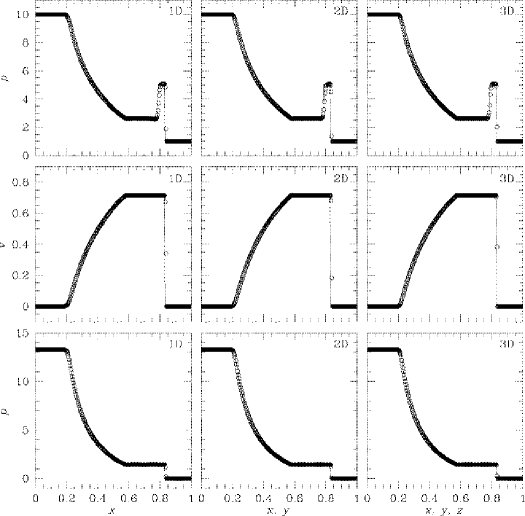
Figure 1: (a) 1D, 2D, and 3D mildly relativistic shock tube tests. The calculations have been done with the initial states in equation (59) using $256$, $256^{2}$, and $256^{3}$ cells. The numerical solutions (open circles) and the exact solutions (solid lines) are plotted at $t=0.4$, $0.4\sqrt{2}$, and $0.4\sqrt{3}$. (b) 1D, 2D, and 3D highly relativistic shock tube tests. The calculations have been done with the initial states in equation (60) using $256$, $256^{2}$, and $256^{3}$ cells. The numerical solutions (open circles) and the exact solutions (solid lines) are plotted at $t=0.4$, $0.4\sqrt{2}$, and $0.4\sqrt{3}$.

In equations (59) and (60), the expressions within inequalities are for one, two, and three dimensions, respectively. The first test involves a mildly relativistic flow and the second test involves a highly relativistic flow. In both tests, we assume the adiabatic index $\gamma=5/3$ and the outflow condition is used for the $x$, $y$, and $z$-boundaries. Both tests were previously considered by several authors (e.g., Martí & Müller, 1996). The estimation of accuracy was done by comparing the numerical solutions with the exact solutions described in Thompson (1986) and Martí & Müller (1994). In Figures 1(a) and (b), our numerical solutions are shown as open circles and the exact solutions are represented by solid lines.

Figure 1(a) shows the mildly relativistic shock tube test done using $256$, $256^{2}$, and $256^{3}$ cells with a Courant constant $C_{\mathrm{Cour}}=0.9$ and the parameters $\varepsilon_{1,5}=0.1$ and $\varepsilon_{2-4}=0$. The plots of one, two, and three-dimensions correspond to times $t=0.4$, $0.4\sqrt{2}$, and $0.4\sqrt{3}$, respectively. Structures such as the shock front, contact discontinuity and rarefaction wave are accurately produced. There are actually slight improvements in accuracy in the multidimensional calculations. Figure 1(b) shows the highly relativistic shock tube test done again using $256$, $256^{2}$, and $256^{3}$ cells with a Courant constant $C_{\mathrm{Cour}}=0.6$ and the parameters $\varepsilon_{1,5}=0.1$ and $\varepsilon_{2-4}=0$. The plots of one, two, and three-dimensions correspond to times $t=0.4$, $0.4\sqrt{2}$, and $0.4\sqrt{3}$, respectively. The flow is more extreme, but the structure is correctly reproduced without spurious oscillations. But in the rest mass density profile the peak does not reach the value of the exact solution due to the coarseness of computational cells. According to our tests, in a one-dimensional calculation, the peak can be accurately reproduced when $2048$ numerical cells are used. There are also improvements in accuracy in the multidimensional calculations.

For a more quantitative comparison, we have calculated the norm errors of the rest mass density, velocity, and pressure for different dimensions. The errors shown in Table 1 are calculated at the same times as in Figure 1. The errors are gradually reduced as the dimensionality increases and demonstrate a good agreement between the numerical and exact solutions. Note that the values of $\|E(p)\|$ exceeding unity are still acceptable because these are from the initial large value of pressure.

3.2 Relativistic Wall Shock

A one-dimensional relativistic wall shock test has been performed in the computational box of $x=[0,1]$. Initially a gas with extreme velocity occupying all numerical cells propagates along the $x$-axis against a reflecting wall placed at $x=1$. As the gas hits the wall, it is compressed and heated and eventually a reverse shock is generated. The initial condition of this test is

$$\left(\rho,v_{x},v_{y},v_{z},p\right)=\left(1,0.999999,0,0,10^{-4}\right)\qquad 0\leq x\leq 1.$$ (61)

The adiabatic index $\gamma=5/3$ is assumed and the inflow boundary condition is used at $x=0$. It is another test which was widely used by several authors (e.g., Donat et al., 1998).

The relativistic jump condition for strong shocks with negligible preshock pressure is given by Blandford & McKee (1976)

$$v_{s}=-\frac{\left(\gamma-1\right)\Gamma v}{\Gamma+1},$$ (62)

$$\rho^{*}=\rho\frac{\gamma\Gamma+1}{\gamma-1},$$ (63)

$$v^{*}=0,$$ (64)

$$p^{*}=\rho\left(\Gamma-1\right)\left(\gamma\Gamma+1\right).$$ (65)

Here, $v_{s}$ is the shock velocity and the superscript $\ast$ represents the postshock quantities, while the quantities without any superscript refer to the preshock gas.

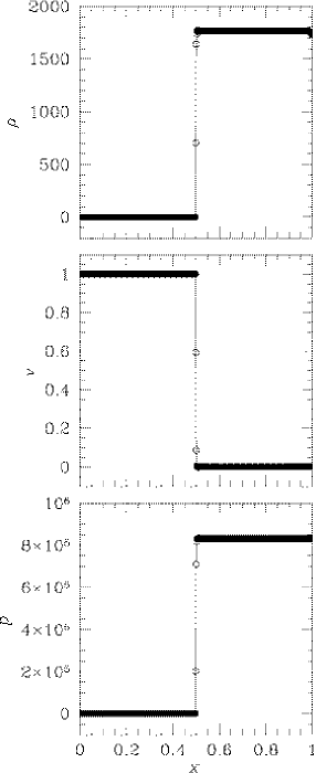
Figure 2: One-dimensional relativistic wall shock test. The calculation has been done with the initial states in equation (61) using $512$ cells. The numerical solution (open circles) and the exact solution (solid lines) are plotted at $t=0.75$.

Figure 2 shows the structure at $t=0.75$ when the reverse shock is located at $x=0.5$. The calculation has been done using $512$ computational cells with a Courant constant $C_{\mathrm{Cour}}=0.9$ and the parameters $\varepsilon_{1,5}=0.3$ and $\varepsilon_{2-4}=0.1$. The numerical solution is drawn with open circles and the exact solution is represented by solid lines. The numerical and exact solutions match exactly without any oscillation or overshoot in the rest mass density, velocity, and pressure profiles.

With different inflow velocities, we have calculated the mean errors in the rest mass density, velocity, and pressure. The errors are calculated for the same time as in Figure 2 and given in Table 2. Note that the order of the mean errors is $10^{-3}$, and that the accuracy does not depend systematically on the investigated Lorentz factor. The mean error in the rest mass density is $\lesssim 0.5\%$ for all the Lorentz factors and about $0.25\%$ for the maximum Lorentz factor. This accuracy is comparable to or better than that of other published upwind scheme codes.

3.3 Relativistic Blast Wave

The propagation of a relativistic blast wave has been tested in the two-dimensional computational box with $x=[0,1]$ and $y=[0,1]$. A gas of high density and pressure is initially confined in a spherical region and the subsequent explosion is allowed to evolve. This makes a spherical blast wave propagate outward. The initial condition of this test is

$$\left(\rho,v_{x},v_{y},v_{z},p\right)=\left\{\begin{array}[]{ll}\left(10,0,0,0,10^{3}\right)&0\leq\sqrt{x^{2}+y^{2}}\leq 1/2,\\ \left(1,0,0,0,1\right)&\mathrm{outside}.\end{array}\right.$$ (66)

The adiabatic index is taken to be $\gamma=4/3$ and the reflecting and outflow boundary conditions are used.

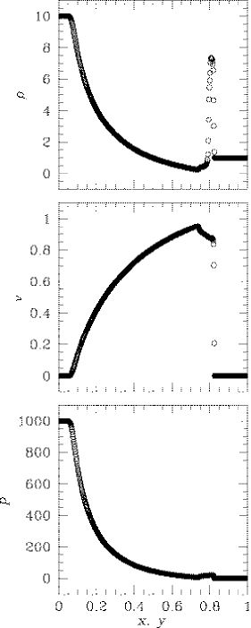
Figure 3: Two-dimensional relativistic blast wave test. The calculation has been done with the initial states in equation (66) using $512^{2}$ cells. The numerical solution (open circles) are plotted at $t=0.7$.

The calculation has been done using $512^{2}$ cells with a Courant constant $C_{\mathrm{Cour}}=0.6$ and the parameters $\varepsilon_{1,5}=0.1$ and $\varepsilon_{2-4}=0$. To test the symmetry properties of the code, the calculation has been stopped before a reverse shock reaches the inner reflecting boundary. Figure 3 shows the profiles of the rest mass density, velocity, and pressure measured along the diagonal line connecting $(0,0)$ and $(1,1)$ at $t=0.7$. The spherical blast wave successfully propagates to a larger radius, and we have found that all structures in it preserve the initial symmetry.

3.4 Relativistic Hawley-Zabusky Shock

In order to test the applicability of the code to complex relativistic flows, we have performed a two-dimensional test simulation of the relativistic version of the Hawley-Zabusky shock. The test was originally suggested by Hawley & Zabusky (1989) for non-relativistic hydrodynamics. Almost the same physical values as in the original paper are used here. Initially a plane-parallel shock with a Mach number $1.2$ propagates along the $x$-axis into two regions of different density. The regions are separated by oblique discontinuity whose inclination is $30^{\circ}$ with respect to the $x$-axis. The density jumps three times across the discontinuity. The initial configuration is summarized as

$$\left(\rho,v_{x},v_{y},v_{z},p\right)=\left\{\begin{array}[]{ll}\left(1,0.6,0,0,0.48\right)&0\leq x\leq 1/16,~{}0\leq y\leq 1,\\ \left(1,0,0,0,0.48\right)&1/16<x\leq\sqrt{3}y+1/4,~{}0\leq y\leq 1,\\ \left(3,0,0,0,0.48\right)&\mathrm{outside}.\end{array}\right.$$ (67)

The adiabatic index $\gamma=1.4$ is used. The inflow and outflow conditions are used at the $x$-boundaries and the reflecting condition is used at the $y$-boundaries.

The simulation has been done in the two-dimensional computational box with $x=[0,8]$ and $y=[0,1]$ using a uniform numerical grid of $2048\times 256$ cells. A Courant constant $C_{\mathrm{Cour}}=0.9$ and the parameters $\varepsilon_{1,5}=0.1$ and $\varepsilon_{2-4}=0$ were used. We have simulated this test until $t=20$ in order to see the long term evolution. The passage of the planar shock through the discontinuity causes the Kelvin-Helmholtz instability to occur along the discontinuity and end up with formation of vortices. The vortices roll up, interact, and merge during the simulation; the detailed morphology and the number of vortices formed are somewhat sensitive to numerical resolution. Figure 4 shows the gray-scale images of the rest mass density at different times ($t=2$, $11$, and $20$). Because all the structures are dragged to the right boundary as time goes on, only the left, middle, and right half of the computational box are shown at $t=2$, $11$, and $20$, respectively. The vortices along the discontinuity are clearly formed and overall the morphology is similar to that of the non-relativistic simulation.

3.5 Relativistic Extragalactic Jets

Finally, in order to test the applicability of the code to realistic relativistic flows, we have simulated a two-dimensional relativistic extragalactic jet propagating into homogeneous medium. The relativistic jet inflows with a velocity $0.99$ to the computational box of $x=[0,4]$ and $y=[0,1]$. The jet has initially radius $1/8$ ($32$ cells) and Mach number $8.76$. The density ratio of the jet to the ambient medium is $0.1$ and the pressure of the jet is in equilibrium with that of the ambient medium. The initial condition for jet inflow and ambient medium is summarized as

$$\left(\rho,v_{x},v_{y},v_{z},p\right)=\left\{\begin{array}[]{ll}\left(1,0.99,0,0,0.1\right)&0\leq x\leq 1/32,~{}0\leq y\leq 1/8,\\ \left(10,0,0,0,0.1\right)&\mathrm{outside}.\end{array}\right.$$ (68)

The adiabatic index $\gamma=4/3$ is used. The inflow and outflow conditions are used at the $x$-boundaries and the reflecting and outflow conditions are used at the $y$-boundaries.

The simulation has been done using a uniform numerical grid of $1024\times 256$ cells with a Courant constant $C_{\mathrm{Cour}}=0.3$ and the parameters $\varepsilon_{1,5}=0.3$ and $\varepsilon_{2-4}=0.1$. Figure 5 shows the gray-scale images of logarithm of the rest mass density, pressure, and Lorentz factor at $t=5$ when the bow shock reaches the right boundary. We can clearly see the dominant structures of bow shock, working surface, contact discontinuity, and cocoon. It is clear that the internal structure of the relativistic jet is less complex compared to that of a non-relativistic jet due to the effects of high Lorentz factor. The overall morphology and dynamics of our simulation match roughly with those of previous works, e.g., Duncan & Hughes (1994), although the initial conditions and the plotted epoch are different.

4 Summary and Discussion

A multidimensional code for special relativistic hydrodynamics was described. It differs from previous codes in the following aspects: 1) It is based on the total variation diminishing (TVD) scheme (Harten, 1983), which is an explicit Eulerian finite difference upwind scheme and an extension of the Roe scheme to second-order accuracy in space and time. 2) It employs a new set of conserved quantities, and so the paper describes a new eigen-structure for special relativistic hydrodynamics. 3) For the Lorentz transformation from the conserved quantities in the reference frame to the physical quantities in the local rest frame, an analytic formula is used.

To demonstrate the performance of the code, several tests were presented, including relativistic shock tubes, a relativistic wall shock, a relativistic blast wave, the relativistic version of the Hawley-Zabusky shock, and a relativistic extragalactic jet. The relativistic shock tube tests showed that the code clearly resolves mildly relativistic and highly relativistic shocks within $2-4$ numerical cells, although it requires more cells for resolving contact discontinuities. The relativistic wall shock test showed that the code correctly captures very strong shocks with very high Lorentz factors. The relativistic blast wave test showed that blast waves propagate through ambient medium while preserving the symmetry. The test simulations of the relativistic version of the Hawley-Zabusky shock and a relativistic extragalactic jet proved the robustness and flexibility of the code, and that the code can be applied to studies of practical astrophysical problems.

The strong points of the new code include the following: 1) Based on the TVD scheme, the code is simple and fast. The core routine of the TVD relativistic hydrodynamics is only about 300 lines long in the three-dimensional version. It runs only about $1.5-2$ times slower than the non-relativistic counterpart (per time step). Yet, tests have shown that the code is accurate and reliable enough to be suited for astrophysical applications. In addition, the use of an analytic formula for Lorentz transformation makes the code robust, so it ran for all the tests we have performed without failing to converge. 2) The code has been built in a way to be completely parallel to the non-relativistic counterpart. So it can be easily understood and used, once one is familiar with the non-relativistic code. In addition, the techniques developed for the non-relativistic code such as parallelization can be imported transparently.

Finally, the code is currently being applied for studies of relativistic jet interactions with inhomogeneous external media and turbulence of relativistic flows. The results will be reported in separate papers.

Table 1: Norm errors for the relativistic shock tube tests

RST	$n_{\mathrm{cell}}$	$\|E(\rho)\|$	$\|E(v)\|$	$\|E(p)\|$
(a) 1D	$256$	1.1688E$-$01	6.0952E$-$02	9.3517E$-$02
2D	$256^{2}$	1.1264E$-$01	6.0586E$-$02	9.6789E$-$02
3D	$256^{3}$	9.1309E$-$02	5.8222E$-$02	8.7047E$-$02
(b) 1D	$256$	1.7506E$-$01	2.6591E$-$02	5.2191E$+$00
2D	$256^{2}$	1.6375E$-$01	1.9552E$-$02	4.3126E$+$00
3D	$256^{3}$	1.3840E$-$01	1.3533E$-$02	2.8773E$+$00

Table 2: Mean errors for the relativistic wall shock tests

$v$	$\Gamma$	$\bar{E}(\rho)$	$\bar{E}(v)$	$\bar{E}(p)$
0.9	2.3	4.7423E$-$03	3.1483E$-$03	5.8100E$-$03
0.99	7.1	3.1938E$-$03	2.3634E$-$03	2.5168E$-$03
0.999	22.4	3.1876E$-$03	2.6687E$-$03	2.5015E$-$03
0.9999	70.7	5.0532E$-$03	4.1790E$-$03	3.8529E$-$03
0.99999	223.6	2.8425E$-$03	2.4914E$-$03	2.1466E$-$03
0.999999	707.1	2.4855E$-$03	2.0237E$-$03	1.8747E$-$03

Figure 4: Two-dimensional relativistic Hawley-Zabusky shock. The simulation has been carried out with the initial configurations in equation (67) using $2048\times 256$ cells. Gray-scale images show the rest mass density at $t=2$, $11$, and $20$ (top to bottom), using linear scales that range from $1.0$ (black) to $6.75$ (white).

Figure 5: Two-dimensional relativistic extragalactic jet. The simulation has been carried out with the initial conditions in equation (68) using $1024\times 256$ cells. Gray-scale images show logarithm of the rest mass density, pressure, and Lorentz factor (top to bottom) at $t=5$, using logarithmic scales that range from $-0.28$ (black) to $1.98$ (white) for log(density), $-1.0$ (black) to $1.30$ (white) for log(pressure), and $0$ (black) to $0.85$ (white) for log(Lorentz factor).

References

- Abramowitz & Stegun (1972) Abramowitz, M. A., & Stegun, I. A. 1972, Handbook of Mathematical Functions (Dover: Dover Publishing Company)
- Aloy et al. (1999) Aloy, M. A., Ibáñez, J. M., Martí, J. M., & Müller, E. 1999, ApJS, 122, 151
- Blandford & McKee (1976) Blandford, R. D., & McKee, C. F. 1976, Phys. Fluids, 19, 1130
- Burrows (2000) Burrows, A. 2000, Nature, 403, 727
- Colella & Woodward (1984) Colella, P., & Woodward, P. R. 1984, J. Comput. Phys., 54, 174
- Dolezal & Wong (1995) Dolezal, A., & Wong, S. S. M. 1995, J. Comput. Phys., 120, 266
- Donat et al. (1998) Donat, R., Font, J. A., Ibáñez, J. M., & Marquina, A. 1998, J. Comput. Phys., 146, 58
- Duncan & Hughes (1994) Duncan, G. C., & Hughes, P. A. 1994, ApJ, 436, L119
- Eulderink & Mellema (1995) Eulderink, F., & Mellema, G. 1995, A&AS, 110, 587
- Harten (1983) Harten, A. 1983, J. Comput. Phys., 49, 357
- Harten et al. (1987) Harten, A., Engquist, B., Osher, S., & Chakravarthy, S. R. 1987, J. Comput. Phys., 71, 231
- Hawley & Zabusky (1989) Hawley, J. F., & Zabusky, N. J. 1989, Phys. Rev. Lett., 63, 1241
- Martí & Müller (1994) Martí, J. M., & Müller, E. 1994, J. Fluid Mech., 258, 317
- Martí & Müller (1996) Martí, J. M., & Müller, E. 1996, J. Comput. Phys., 123, 1
- Martí & Müller (2003) Martí, J. M., & Müller, E. 2003, Living Rev. Relativity, 6, 7
- Mészáros (2002) Mészáros, P. 2002, ARA&A, 40, 137
- Mirabel & Rodríguez (1999) Mirabel, I. F., & Rodríguez, L. F. 1999, ARA&A, 37, 409
- Roe (1981) Roe, P. L. 1981, J. Comput. Phys., 43, 357
- Ryu et al. (1993) Ryu, D., Ostriker, J. P., Kang, H., & Cen, R. 1993, ApJ, 414, 1
- Schneider et al. (1993) Schneider, V., Katscher, U., Rischke, D. H., Waldhauser, B., Maruhn, J. A., & Munz, C.-D. 1993, J. Comput. Phys., 105, 92
- Strang (1968) Strang, G. 1968, SIAM J. Numer. Anal., 5, 506
- Thompson (1986) Thompson, K. W. 1986, J. Fluid Mech., 171, 365
- Wilson & Mathews (2003) Wilson, J. R., & Mathews, G. J. 2003, Relativistic Numerical Hydrodynamics (Cambridge: Cambridge Univ. Press)
- Zensus (1997) Zensus, J. A. 1997, ARA&A, 35, 607