Chemical Composition of Two H II Regions in NGC 6822 Based on VLT Spectroscopy

Abstract

We present long slit spectrophotometry of regions V and X of the local group irregular galaxy NGC 6822. The data consist of VLT FORS observations in the 3450 to 7500 Å range. We have obtained electron temperatures and densities using different line intensity ratios. We have derived the He, C, and O abundances relative to H based on recombination lines, the abundance ratios among these elements are almost independent of the temperature structure of the nebulae. We have also determined the N, O, Ne, S, Cl, and Ar abundances based on collisionally excited lines, the ratios of these abundances relative to that of H depend strongly on the temperature structure of the nebulae. The chemical composition of NGC 6822 V is compared with those of the Sun, the Orion nebula, NGC 346 in the SMC, and 30 Doradus in the LMC. The O/H value derived from recombination lines is in good agreement with the value derived by Venn et al. (2001) from two A type supergiants in NGC 6822.

1 Introduction

The main aim of this paper is to make a new determination of the chemical abundances of the two brightest H II regions in NGC 6822: regions V and X (Hubble, 1925). We include the following improvements over previous determinations: the consideration of the temperature inhomogeneities that affects the helium and heavy elements abundance determinations, the derivation of the O and C abundances from recombination line intensities, the consideration of the collisional excitation of the triplet He I lines from the $2^{3}$S level by determining the helium abundance from many line intensity ratios, and the study of the $2^{3}$S level optical depth effects on the intensity of the triplet lines by observing a large number of singlet and triplet lines of He I.

We are interested in three applications based on the abundance determinations: the determination of $t^{2}$, the comparison of the nebular abundances derived in this paper with the stellar abundances of supergiant stars in NGC 6822 derived elsewhere (Muschielok et al., 1999; Venn et al., 2001; Venn & Miller, 2002; Venn et al., 2004), and to provide accurate abundances for galactic chemical evolution models of this object (e. g. Carigi et al., 2005a).

NGC 6822 is an irregular galaxy member of the local group particularly suited for chemical evolution models because its star formation history is well known (Wyder, 2001), and apparently has not been affected by tidal effects, therefore its chemical composition might permit to decide if outflows to the intergalactic medium have occurred in this galaxy.

The importance of outflows to the intergalactic medium from nearby irregular galaxies depends on many factors, like their total mass, the distribution in time and space of their star formation, and tidal effects (e.g. Legrand et al., 2001; Tenorio-Tagle et al., 2003; Martin, 2003; Fragile et al., 2004, and references therein).

NGC 6822 apparently has not been affected by tidal effects from the main galaxies of the local group: the Milky Way and M31 (Sawa & Fujimoto, 2005). NGC 6822 is located at 495 kpc from our Galaxy and is moving away from it at a radial velocity of 44 km s^-1 (Trimble, 2000). NGC 6822 is also located at 880 kpc from M31, and it is separated from M31 by more than 90 degrees in the sky (Trimble, 2000).

In sections 2 and 3 the observations and the reduction procedure are described. In section 4 temperatures and densities are derived from four and three different intensity ratios respectively; also in this section, the mean square temperature fluctuation, $t^{2}$, is determined from the O II/[O III] line intensity ratios and from the difference between $T$(He I) and $T$([O III+O II]). In section 5 we determine ionic abundances based on recombination lines that are almost independent of the temperature structure, we determine also ionic abundances based on ratios of collisionally excited lines to recombination lines that do depend on the temperature structure of the nebula. In section 6 we determine the total abundances. In sections 7 and 8 we present the discussion and the conclusions.

2 Observations

The observations were obtained with the Focal Reducer Low Dispersion Spectrograph 1, FORS1, at the VLT Melipal Telescope in Chile. We used three grisms: GRIS_-600B+12, GRIS_-600R+14 with filter GG435, and GRIS_-300V with filter GG375 (see Table 1).

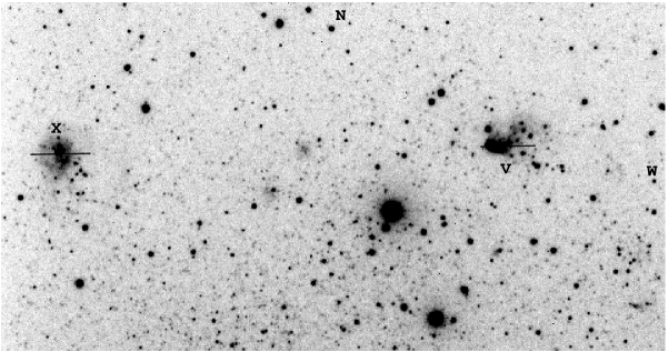
Figure 1: VLT image of regions V and X in NGC 6822. The image of $277"\times 145"$ is centered at $\alpha=19^{\rm h}44^{\rm m}57.4^{\rm s}$, $\delta=-14^{\rm o}43^{\prime}26"$ (J2000), and was taken with a filter that suppresses light bluer than 4350 Å. The extraction apertures are shown in the figure. The aperture for region V is centered at $\alpha=19^{\rm h}44^{\rm m}52.40^{\rm s}$, $\delta=-14^{\rm o}43^{\prime}13.4"$, with a size of $22.4"\times 0.51"$; and the aperture for region X is centered at $\alpha=19^{\rm h}45^{\rm m}05.23^{\rm s}$, $\delta=-14^{\rm o}43^{\prime}16.7"$, with a size of $24.6"\times 0.51"$. The position angle for the long slit was $91^{\rm o}$.

The slit was oriented almost east-west (position angle 91^o) to observe the brightest regions of NGC 6822 V and of 6822 X simultaneously. The linear atmospheric dispersion corrector, LACD, was used to keep the same observed region within the slit regardless of the air mass value. The slit width was set to 0.51” and the slit length was 410”. The aperture extractions were made for an area of 22.4” $\times$ 0.51” for region V and an area of 24.6” $\times$ 0.51” for region X, covering the brightest parts of both regions (see Figure 1). The resolution for the emission lines observed with the blue grism is given by $\Delta\lambda\sim\lambda/1300$, with the red grism is given by $\Delta\lambda\sim\lambda/1700$, and with the low resolution grism is given by $\Delta\lambda\sim\lambda/700$. The average seeing during the observations amounted to 0.8”.

The spectra were reduced using IRAF reduction packages, following the standard procedure of bias subtraction, aperture extraction, flatfielding, wavelength calibration and flux calibration. For flux calibration the standard stars LTT 2415, LTT 7389, LTT 7987 and EG 21 were used (Hamuy et al., 1992, 1994). The observed spectra are presented in Figures 2 and 3.

3 Line Intensities, Reddening Correction, and Radial Velocities

Line intensities were measured integrating all the flux in the line between two given limits and over a local continuum estimated by eye. In the few cases of line-blending, the line flux of each individual line was derived from a multiple Gaussian profile fit procedure. All these measurements were carried out with the splot task of the IRAF package.

The reddening coefficients, $C$(H$\beta$)’s, were determined by fitting the observed $I$(H$\beta$)/$I$(H Balmer lines) ratios to the theoretical ones computed by Storey & Hummer (1995) for $T_{e}$ = 10,000 K and $N_{e}$ = 100 cm^-3, (see below) and assuming the extinction law of Seaton (1979).

Table 2 presents the emission line intensities of the NGC 6822 H II regions. The first two columns include the adopted laboratory wavelength, $\lambda$, and the identification for each line. The third and fourth columns include the observed flux relative to H$\beta$, $F(\lambda$), and the flux corrected for reddening relative to H$\beta$, $I(\lambda$), for region V. The last two columns include the same information as the previous two but for region X. To combine all the line intensities, from the three different instrumental settings, on the same scale, we multiplied the intensities in each setting by a correction factor obtained from the lines present in more than one setting. The errors were estimated by comparing all the measured H line intensities, with those predicted by the computations of Storey & Hummer (1995) and by assuming that the signal to noise increases as the square root of the measured flux. These estimates are in agreement with the differences found when comparing the line fluxes observed in different exposures.

4 Physical Conditions

4.1 Temperatures and densities

The temperatures and densities presented in Table 3 were derived from the line intensities presented in Table 2. The determinations were carried out based on the temden IRAF subroutine; this subroutine models a 5-, 6-, or 8-level ion to derive these quantities.

To compute $T$([O II]), the contribution to the intensities of the $\lambda\lambda$ 7319, 7320, 7331, and 7332 [O II] lines due to recombination was taken into account based on the following equation:

$$I_{R}(7319+7320+7331+7332)/I({\rm H\beta})=9.36(T/10^{4})^{0.44}\times{\rm{O}}^{++}/{\rm{H}}^{+}$$ (1)

(see Liu et al., 2000).

Similarly, to compute $T$([N II]), the contribution to the intensity of the $\lambda$ 5755 [N II] line due to recombination was taken into account based on the following equation:

$$I_{R}(5755)/I({\rm H\beta})=3.19(T/10^{4})^{0.30}\times{\rm{N}}^{++}/{\rm{H}}^{+}$$ (2)

(see Liu et al., 2000).

4.2 Temperature variations

To derive the ionic abundance ratios the average temperature, $T_{0}$, and the mean square temperature fluctuation, $t^{2}$, were used. These quantities are given by

$$T_{0}(N_{e},N_{i})=\frac{\int T_{e}({\bf r})N_{e}({\bf r})N_{i}({\bf r})dV}{\int N_{e}({\bf r})N_{i}({\bf r})dV}$$ (3)

and

$$t^{2}=\frac{\int(T_{e}-T_{0})^{2}N_{e}N_{i}dV}{T_{0}^{2}\int N_{e}N_{i}dV},$$ (4)

respectively, where $N_{e}$ and $N_{i}$ are the electron and the ion densities of the observed emission line and $V$ is the observed volume (Peimbert, 1967).

To determine $T_{0}$ and $t^{2}$ we need two different methods to derive $T_{e}$: one that weighs preferentially the high temperature regions and one that weighs preferentially the low temperature regions (Peimbert, 1967). In this paper we have used the temperature derived from the ratio of the [O III] $\lambda\lambda$ 4363, 5007 lines, $T_{(4363/5007)}$, that is given by

$$T_{(4363/5007)}=T_{0}\left[1+{\frac{1}{2}}\left({\frac{91300}{T_{0}}}-3\right)t^{2}\right]$$ (5)

and the temperature derived from the ratio of the recombination lines of multiplet 1 of O II to the collisionally excited lines of [O III] that is given by (see Peimbert et al., 2004, equations 8-12)

$$T_{({\rm O\,\scriptscriptstyle II}\,rec/{\rm O\,\scriptscriptstyle III}\,coll)}=T_{(4649/5007)}=f_{1}(T_{0},t^{2}).$$ (6)

Using the O recombination lines of Region V, based on these equations, we obtain $T_{0}=10100$ K and $t^{2}=0.092\pm 0.026$. Since in this object most of the oxygen is twice ionized (see section 5.3), this $t^{2}$ value is representative for the whole H II region.

It is also possible to derive the $t^{2}$ value from the analysis of the helium lines (see section 5.1). The resulting values are: $t^{2}=0.060\pm 0.026$ and $0.056\pm 0.045$ for regions V and X respectively. For region V we combine the oxygen and the helium determinations and adopt $t^{2}=0.076\pm 0.018$; for region X we simply adopt the $t^{2}$ helium determination. The $t^{2}$ values derived for regions V and X are somewhat larger than those derived for Galactic H II regions, that typically are in the 0.03 to 0.04 range (Esteban et al., 2005) but are similar to those derived in giant extragalactic H II regions (Esteban et al., 2002; Peimbert, 2003).

5 Ionic Chemical Abundances

5.1 Helium ionic abundances

To obtain He⁺/H⁺ values we need a set of effective recombination coefficients for the He and H lines, the contribution due to collisional excitation to the helium line intensities, and an estimate of the optical depth effects for the helium lines. The recombination coefficients used were those by Storey & Hummer (1995) for H, and those by Smits (1996) and Benjamin, Skillman, & Smits (1999) for He. The collisional contribution was estimated from Sawey & Berrington (1993) and Kingdon & Ferland (1995). The optical depth effects in the triplet lines were estimated from the computations by Benjamin, Skillman, & Smits (Benjamin et al.2002).

Before using the helium lines, much in the same way as we do for hydrogen lines, we need to correct them for underlying absorption and, in the cases of $\lambda$ 3889 and $\lambda$ 4713, for blends. To correct the blue lines, $\lambda<5000$ Å, for underlying absorption we used the values determined by González Delgado et al. (1999), for the redder lines we used values determined by Cerviño M. (private communication) based on the paper by González Delgado et al. (2005). It should be noted that the underlying absorption in the helium lines scales, in the same way as it does in the hydrogen lines, as a fraction of the correction to H$\beta$. After discarding the lines that could not be easily unblended or those for which there is no accurate atomic data, the remaining lines are presented in Table 4.

We have many measured helium lines, each of them with a different dependence on temperature and density. In principle one can find He I line ratios that will allow to measure temperature or density. In practice the dependence of each ratio is weak, also each ratio depends simultaneously on $T_{0}$, $t^{2}$, $N_{e}$, and $\tau_{3889}$; making the determinations, obtained from any one ratio, to have large error bars. In order to optimize our data we used a maximum likelihood method (MLM) to search for the physical and chemical conditions ($T_{0}$, $t^{2}$, $\tau_{3889}$, and He⁺/H⁺) that would give us the best simultaneous fit to all the measured lines (see , Peimbert, Peimbert, & Ruiz2000).

For these objects the MLM can not determine the electron density with high enough accuracy to be useful; therefore we have adopted the electron densities derived from collisionally excited lines. Based on Table 3 we adopted $N_{e}=175\pm 30$ cm^-3 and $N_{e}=30\pm 30$ cm^-3, for regions V and X respectively, to help with the determinations.

To help break the degeneracy on $T_{0}$ and $t^{2}$ we need to use an additional temperature; since $T$(He I) weighs preferentially the low temperature regions, we used a temperature that weighs preferentially the high temperature regions (see section 4.2). In order for this temperature to be representative of the whole region we used a weighted average of $T$([O II]) and $T$([O III]) (see , Peimbert et al.2002): for region V we used $T$([O III+O II])$=12000$ K and for region X we used$T$([O III+O II])$=12250$ K.

From these line intensities, densities, temperatures and the MLM we obtained the He abundances presented in Table 5, a $t^{2}=0.060\pm 0.026$ for region V, and a $t^{2}=0.056\pm 0.045$ for region X.

5.2 C and O ionic abundances from recombination lines

The C⁺⁺ abundance was derived from the $\lambda 4267$ Å line of C II and the effective recombination coefficients computed by Davey, Storey, & Kisielius (2000) for Case A and $T=10,000$ K. We only observe the $\lambda 4267$ Å line in region V, the expected flux of this line for region X would produce a S/N$\approx$1, making it impossible to measure.

The O⁺⁺ abundance was derived from multiplet 1 of O II (Peimbert, Storey, & Torres-Peimbert, 1993; Storey, 1994). The multiplet consists of 8 lines and the sum of their intensities, $I$(sum), normalized to $I$(H$\beta$), is independent of the electron density. On the other hand the normalized intensity of each of the eight lines does depend on the electron density (Ruiz et al., 2003). It is rarely possible to measure all the lines of this multiplet, and frequently it is necessary to estimate the intensities of the unobserved (or blended) lines.

As with C II, we only observe O II recombination lines on region V. Of the 8 lines of multiplet 1 we only detect 4; which, due to the dispersion of our observations, are blended into 2 pairs $\lambda\lambda$ 4639+42 and 4649+51 Å.

Ruiz et al. (2003) found that, for typical H II region densities, the relative intensities of the lines of the multiplet deviate from the LTE computation predictions. In order to determine what fraction of the intensity of the whole multiplet is emitted in these 4 lines it is necessary to determine the density dependence of each of these lines. Ruiz et al. present the density dependence of $I$(4649)/$I$(sum). In order to determine the density relations, for all the lines of the multiplet, in Figures 4, 5, 6, and 7 we present plots of the data listed by Ruiz et al. in their Table 8 for the four sets of lines of multiplet 1 that originate in a given upper level (note that our Figure 7 is the same as Figure 2 by Ruiz et al.). From Figures 4 to 7 it can be seen that the intensity of the lines that originate in the 3p ⁴D${}^{0}_{3/2}$ and 3p ⁴D${}^{0}_{1/2}$ energy levels decreases with increasing local density, while the intensity of those lines that originate in the 3p ⁴D${}^{0}_{7/2}$ increases with increasing density. This is due to the effect of collisional redistribution that increases the population of the high statistical weight levels at the expense of the low statistical weight ones. Note that the intensity of the lines that originate from the 3p ⁴D${}^{0}_{5/2}$ energy level depend weakly on the electron density.

Based on Figures 4 to 7 and a relationship of the type

$$\left[\frac{I(line)}{I({\rm sum})}\right]_{obs}=\left[\frac{I(line)}{I({\rm sum})}\right]_{LTE}+\frac{\left[\frac{I(line)}{I({\rm sum})}\right]_{cas}-\left[\frac{I(line)}{I({\rm sum})}\right]_{LTE}}{\left[1+\frac{N_{e}({\rm FL})}{N_{e}({\rm crit})}\right]},$$ (7)

we have obtained the following equations:

$$\left[\frac{I(4651+74)}{I({\rm sum})}\right]_{obs}=0.101+\frac{0.144}{\left[1+N_{e}({\rm FL})/1325\right]},$$ (8)

$$\left[\frac{I(4639+62+96)}{I({\rm sum})}\right]_{obs}=0.201+\frac{0.205}{\left[1+N_{e}({\rm FL})/1325\right]},$$ (9)

$$\left[\frac{I(4642+76)}{I({\rm sum})}\right]_{obs}=0.301-\frac{0.057}{\left[1+N_{e}({\rm FL})/1325\right]},$$ (10)

and

$$\left[\frac{I(4649)}{I({\rm sum})}\right]_{obs}=0.397-\frac{0.292}{\left[1+N_{e}({\rm FL})/1325\right]},$$ (11)

where the first term on the right hand side corresponds to the LTE ratio presented by Wiese et al. (1996) and the second term takes into account the deviation from LTE. The intensity of the lines originating from the same upper level is constant and depends only on the ratio of the Einstein A coefficients for each level; thus $I(4651)$:$I(4674)$ is 0.844:0.156, $I(4639)$:$I(4662)$:$I(4696)$ is 0.455:0.506:0.039, and $I(4642)$:$I(4676)$ is 0.742:0.258; since $\lambda 4649$ Å is the only line originating from the 3p ⁴D${}^{0}_{7/2}$ upper level it will contain all the photons originating from this level.

Based on equations 8 to 11, the relative intensities of the lines originating from the same upper level, and the O II lines presented in Table 2 we have determined the $I$(sum) value for multiplet 1 which amounts to $I$(sum)/ $I$(H$\beta$)=0.0023 . We have derived the O⁺⁺ abundance presented in Table 5 from $I$(sum) and the effective recombination coefficient for multiplet 1 computed by Storey (1994) under the assumption of Case B for $T_{e}=10,000$ K and $N_{e}$ = 100 cm^-3.

5.3 Ionic abundances from collisionally excited lines

The values presented in Table 6 for $t^{2}=0.00$ were derived with the IRAF task abund, using only the low- and medium-ionization zones. abund requires as inputs a temperature and a density for each zone as well as the intensities of the observed collisionally excited lines relative to H$\beta$. These values are combined with a model of a 5-, 6-, or 8-level ion to determine the abundances. The low and medium ionization zones of abund correspond to the low and high ionization zones of this paper. For Region V we used $T_{low}=13000\;$K, $T_{high}=11900\;$K, and $N_{e\;low}=N_{e\;high}=175\;$cm^-3; and for Region X we used $T_{low}=13300\;$K, $T_{high}=12000\;$K, and $N_{e\;low}=N_{e\;high}=30\;$cm^-3.

To derive the abundances for $t^{2}>0.00$ we used the abundances for $t^{2}=0.00$ corrected by the formulation for $t^{2}>0.00$ presented by Peimbert & Costero (1969) (see also Peimbert et al., 2004). To derive abundances for other $t^{2}$ values it is possible to interpolate or to extrapolate the values presented in Table 6.

6 Total Abundances

To obtain the C and N gaseous abundances the following equations were adopted

$$\frac{N(\rm C)}{N(\rm H)}=ICF({\rm C})\frac{N({\rm C^{++}})}{N(\rm H^{+})}$$ (12)

and

$$\frac{N(\rm N)}{N(\rm H)}=ICF({\rm N})\frac{N({\rm N^{+}})}{N(\rm H^{+})},$$ (13)

the $ICF$(C) value was obtained from Garnett et al. (1995) and amounts to 0.07 dex. The $ICF$(N) value was obtained from the models by Moore et al. (2004) and amounts to 1.13 dex for region V and to 0.91 dex for region X. Note that the $ICF$(N) value predicted by Peimbert & Costero (1969) is given by $N$(O)/$N$(O⁺) and amounts to 0.97 dex for region V and to 0.75 dex for region X; the $ICF$(N) formula by Peimbert and Costero is a very good approximation for H II regions with low degree of ionization but becomes only fair for H II regions with high degree of ionization. The $ICF$(N) for models in which a large fraction of the ionizing photons escape from the H II region becomes even larger than those predicted by the models by Moore et al. (2004), see for example the results for NGC 346 obtained by (Relaño et al.2002).

The gaseous abundances for O and Ne were obtained from the following equations (Peimbert & Costero, 1969)

$$\frac{N(\rm O)}{N(\rm H)}=\frac{N({\rm O^{+}})+N(\rm O^{++})}{N(\rm H^{+})}$$ (14)

and

$$\frac{N(\rm Ne)}{N(\rm H)}=\left(\frac{N({\rm O^{+}})+N(\rm O^{++})}{N(\rm O^{++})}\right)\frac{N(\rm Ne^{++})}{N(\rm H^{+})}.$$ (15)

The gaseous abundances of S, Cl, and Ar, were obtained from the following equations:

$$\frac{N(\rm S)}{N(\rm H)}=ICF({\rm S})\frac{N({\rm S^{+}})+N(\rm S^{++})}{N(\rm H^{+})},$$ (16)

$$\frac{N(\rm Cl)}{N(\rm H)}=ICF({\rm Cl})\frac{N({\rm Cl^{++}})}{N(\rm H^{+})},$$ (17)

and

$$\frac{N(\rm Ar)}{N(\rm H)}=ICF({\rm Ar})\frac{N({\rm Ar^{++}})+N(\rm Ar^{3+})}{N(\rm H^{+})}.$$ (18)

The $ICF$(S) values were estimated from the models by Garnett (1989) and amount to 0.22 dex for region V and to 0.10 dex for region X. The $ICF$(Cl) values amount to 0.05 dex for regions V and X and were obtained by averaging the observed $N$(Cl⁺ + Cl⁺⁺ + Cl⁺³)/ $N$(Cl⁺⁺) values obtained for Orion, 30 Doradus, and NGC 3576 (Esteban et al., 2004; Peimbert, 2003; García-Rojas et al., 2004). The ionization correction factor due to the Ar⁺ fraction was estimated from $ICF$(Ar) = 1/[1 - O⁺/O] (Liu et al., 2000) and amounts to 0.05 dex and 0.09 dex for regions V and X respectively.

Based on the previous considerations, we present the total gaseous abundances of regions V and X in Tables 7 and 8 respectively. The errors for region X are larger than those for region V because the brightness of region X is about three times smaller than that of region V. Within the errors the abundances of both regions are similar. We need observations of higher quality, than those presented in this paper, to establish the presence of abundance variations among H II regions in NGC 6822.

In Table 9 we present the adopted total abundances for NGC 6822. To obtain the total O and C abundances we have to add a correction to the gaseous abundance due to the presence of dust. Following Esteban et al. (1998) this corrections amount to 0.08 dex for O and 0.10 dex for C.

We have also computed the hydrogen, helium, and heavy elements by mass for NGC 6822 V and amount to: $X$ = 0.7501, $Y$ = 0.2433, and $Z$ = 0.0066. The $Z$ value was computed from the C, N, O, Ne, and Fe abundances (see Table 9, where the Fe abundance comes from stellar data by Venn et al., 2001) and assuming that they constitute 83.3$\%$ of the total $Z$ value. This fraction was obtained by assuming that all the other heavy elements in NGC 6822 present the same abundances relative to O than in the Sun as presented by Asplund et al. (2005).

7 Discussion

7.1 Comparison with other nebular abundance determinations

There have been seven O/H determinations for Hubble V carried out by Smith (1975); Lequeux et al. (1979); Talent (1980); Peimbert & Spinrad (1970); Pagel et al. (1980); Skillman et al. (1989) and Hidalgo-Gámez et al. (2001) that amounted to 12 + log O/H = 8.45, 8.28, 8.20, 8.10, 8.19, 8.20 and 8.10 respectively; these determinations were made based on the $T$(O III) temperature and under the assumption that $t^{2}=0.00$. Statistical errors are typically about 0.1 dex, so to a first approximation there is good agreement among the seven determinations. A second look reveals a systematic difference, the first three determinations were made with the image intensified dissector scanner, IIDS, and yield an average value of 8.31 dex, while the other four were made with other detectors and yield an average value of 8.15 dex, the difference is real and is mainly due to the non-linearity of the IIDS detector (Peimbert & Torres-Peimbert, 1987).

In Tables 7 and 8 we compare our determinations with those of Lequeux et al. (1979) and Hidalgo-Gámez et al. (2001) for $t^{2}=0.00$. As expected our values for O/H and Ne/H are in better agreement with those by Hidalgo-Gámez et al. (2001). As mentioned above the reason is the non linearity of the IIDS detector that increases the difference between weak lines and strong lines, thus yielding lower temperatures and consequently larger O/H and Ne/H values. For Region V this non linearity also yields lower He⁺/H⁺ values , because the helium line intensities are weaker than the H line intensities. For region X the He⁺/H⁺ differences are not significative because the observational errors are larger than the differences predicted by the non-linearity. The smaller errors for region V than for region X are due to the higher luminosity of region V, as can be seen in Table 2. Due to the smaller errors in the line intensities of region V, we took the abundances of this region as representatives of the whole galaxy.

7.2 Comparison with stellar abundance determinations

The stars and H II regions of NGC 6822 have reliable O/H determinations that can be compared. In Table 10 we present the O/H abundances derived in this paper for Hubble V with those derived by Venn et al. (2001) for two A type supergiants; the A supergiants were formed a few million years ago, therefore we expect them to have the same abundances as the H II regions. We find excellent agreement between the stellar O/H values and the ones found using recombination lines; alternatively, the agreement with the values derived using collisionally excited lines ($t^{2}=0.00$) is poor. Also, based on three B supergiant stars in NGC 6822 Muschielok et al. (1999) find a Fe/H of -0.5 $\pm$ 0.2 dex relative to the Sun in excellent agreement with the results of Venn et al. (2001) for two A type supergiants.

7.3 Comparison with the Magellanic Clouds, the Orion nebula, and the Sun

Also in Table 9 we present the Orion and the solar abundances for comparison. For Orion: Fe comes from Cunha & Lambert (1994) based on Orion B stars, and all the other elements from Esteban et al. (2004). For the Sun: He comes from Christensen-Dalsgaard (1998), and all the other elements from Asplund et al. (2005), the solar abundances are the photospheric ones with the exception of He that corresponds to the initial He abundance and of Cl that comes from meteoritic data.

We consider that the Orion nebula is more representative of the present chemical composition of the solar vicinity than the Sun for two main reasons: a) the Sun appears deficient by roughly 0.1 dex in O, Si, Ca, Sc, Ti, Y, Ce, Nd and Eu, compared with its immediate neighbors with similar iron abundances (Allende Prieto et al., 2004), the probable reason for this difference is that the Sun is somewhat older than the comparison stars; and b) all the chemical evolution models of the Galaxy predict a steady increase of the O/H ratio in the solar vicinity with time, for example the chemical evolution models of the solar vicinity presented by Carigi (2003) and Carigi et al. (2005b) indicate that the O/H value in the solar vicinity has increased by 0.13 dex since the Sun was formed.

There are two independent methods to determine the O/H ratio in the ISM of the solar vicinity: a) From the solar 12 + log O/H ratio by Asplund et al. (2005) that amounts to 8.66 and taking into account the increase of the O/H ratio due to galactic chemical evolution since the Sun was formed, that according to state of the art chemical evolution models of the Galaxy amounts to 0.13 dex (e. g. Carigi et al., 2005b), we obtain a value of 8.79 dex; b) The O/H value derived by Esteban et al. (2005), based on the galactic gradient determined from the O II recombination lines observed in H II regions, that amounts to 8.79 dex in perfect agreement with the value based on the solar abundance and the chemical evolution of the Galaxy.

Lee et al. (2005) have derived a value of 12 + log O/H = 8.45 for the A supergiant WLM 15 in the Local Group dwarf irregular galaxy WLM, they have also derived a value of 12 + log O/H = 7.83 for two H II regions in the same galaxy based on the $T$(4363/5007) temperature and under the assumption that $t^{2}=0.00$. The discrepancy between these two determinations can be reduced by assuming that 20% of the oxygen atoms are trapped in dust grains inside H II regions, as is the case in the Orion nebula (Esteban et al., 1998), and by considering the presence of spatial temperature fluctuations. A typical correction for spatial temperature fluctuations based on the recombination lines of O II in NGC 6822V and other extragalactic H II regions (Esteban et al., 2002) amounts to about 0.25 dex.

8 Conclusions

We show that the ratios of the lines of multiplet 1 of O II are not constant, but instead they depend on density. Only at high densities they coincide with the ratios predicted using LTE. The same arguments can probably be made for most recombination lines from other multiplets of heavy elements.

We present a set of empirical equations to determine the O abundances from recombination lines of multiplet 1 of O II. These equations are useful for those cases in which not all the lines of the multiplet are observed.

We derive for the first time the C/H and O/H abundances of NGC 6822 based on recombination lines. We have also derived the N, O, Ne, S, Cl, and Ar abundances based on collisionally excited lines for $t^{2}=0.00$ and for $t^{2}>0.00$ (the $t^{2}$ derived in this paper).

The O/H ratio derived from O II recombination lines is 0.26 dex higher than that derived from [O III] $\lambda\lambda 4363,4959,5007$ collisionally excited lines under the assumption that $t^{2}=0.00$ (that is, by adopting the $T$(4363/5007) temperature).

We have found that, in NGC 6822, the O/H abundance ratio derived from O II recombination lines is in very good agreement with the O/H ratios derived from A-type supergiants, while the O/H abundances derived from collisionally excited lines are not. This result is qualitatively equivalent to that found for the solar vicinity by Esteban et al. (2004) and Carigi et al. (2005a); these authors find that the H II region O/H recombination abundances are in agreement with the O/H solar abundances after considering the O/H enrichment predicted by a chemical evolution model of the Galaxy, while the H II region O/H abundances derived from collisionally excited lines (assuming $t^{2}=0.00$) are not.

The high N/O ratio places NGC 6822 on the plateau formed by irregular galaxies in the N/O-O/H diagram, which implies that a large fraction of the N present in this object is already due to secondary production. From the O/H, C/O, and N/O values it follows that NGC 6822 is considerably more chemically evolved than the SMC. Chemical evolution models for NGC 6822 are presented elsewhere (Carigi et al., 2005a).

We are grateful to Leticia Carigi and Pedro Colín for several useful discussions. We are also grateful to Miguel Cerviño for providing us with the correction for underlying absorption of the He I red lines. We also acknowledge several excellent suggestions by Richard B.C. Henry, who was the referee of this paper, for a careful reading of the manuscript and several useful suggestions. AP received partial support from DGAPA UNAM (grant IN 118405). MP received partial support from DGAPA UNAM (grant IN 114601). MTR received partial support from FONDAP(15010003), and Fondecyt(1010404).

Table 1: Journal of Observations

Date	$\lambda$ (Å)		Exp. Time (s)
2002 Sept 10	3450–	5900	3$\times$720
2002 Sept 10	5250–	7450	3$\times$600
2002 Sept 12	3850–	7500	1$\times$300

Table 2: Line Intensities for Regions V and X

			Region V					Region X
$\lambda$	Id.	$F(\lambda)$		$I(\lambda)$				$F(\lambda)$		$I(\lambda)$
3634	He I	0.	12	0.	18 $\pm$	0.07		$\cdots$		$\cdots$
3687	H 19	0.	42	0.	62 $\pm$	0.12		$\cdots$		$\cdots$
3692	H 18	0.	51	0.	75 $\pm$	0.13		$\cdots$		$\cdots$
3697	H 17	0.	53	0.	77 $\pm$	0.14		$\cdots$		$\cdots$
3704	H 16	0.	85	1.	24 $\pm$	0.17		1.	01	1.	31 $\pm$	0.29
3712	H 15	0.	76	1.	10 $\pm$	0.16		0.	93	1.	21 $\pm$	0.26
3722	H 14	1.	14	1.	64 $\pm$	0.20		1.	12	1.	44 $\pm$	0.30
3726	[O II]	26.	90	38.	90 $\pm$	1.00		46.	80	60.	40 $\pm$	2.00
3729	[O II]	37.	80	54.	60 $\pm$	1.20		66.	90	86.	30 $\pm$	2.50
3734	H 13	1.	28	1.	85 $\pm$	0.21		1.	32	1.	70 $\pm$	0.33
3750	H 12	1.	44	2.	06 $\pm$	0.22		2.	68	3.	43 $\pm$	0.47
3771	H 11	2.	02	2.	87 $\pm$	0.26		2.	32	2.	95 $\pm$	0.44
3798	H 10	2.	49	3.	51 $\pm$	0.28		3.	81	4.	82 $\pm$	0.55
3820	He I	0.	42	0.	58 $\pm$	0.12		0.	91	1.	15 $\pm$	0.27
3835	H 9	4.	03	5.	61 $\pm$	0.36		4.	29	5.	39 $\pm$	0.58
3869	[Ne III]	25.	30	34.	70 $\pm$	0.90		21.	90	27.	30 $\pm$	1.30
3889	H 8+He I	11.	60	16.	10 $\pm$	0.60		13.	90	17.	10 $\pm$	1.00
3967	[Ne III]+H 7+He I	19.	00	25.	40 $\pm$	0.70		18.	90	23.	00 $\pm$	1.20
4026	He I	1.	21	1.	60 $\pm$	0.18		1.	40	1.	69 $\pm$	0.31
4069	[S II]	0.	75	0.	97 $\pm$	0.14		$\cdots$		$\cdots$
4076	[S II]	0.	17	0.	22 $\pm$	0.07		$\cdots$		$\cdots$
4101	H$\delta$	19.	20	24.	70 $\pm$	0.70		20.	20	24.	00 $\pm$	1.20
4144	He I	0.	19	0.	24 $\pm$	0.07		$\cdots$		$\cdots$
4146+53	O II+Ne II	0.	13	0.	16 $\pm$	0.06		$\cdots$		$\cdots$
4192+96	O II	0.	12	0.	15 $\pm$	0.05		$\cdots$		$\cdots$
4267	C II	0.	07	0.	09 $\pm$	0.02		$\cdots$		$\cdots$
4340	H$\gamma$	39.	20	47.	00 $\pm$	1.00		41.	40	46.	90 $\pm$	1.70
4363	[O III]	4.	87	5.	79 $\pm$	0.33		4.	21	4.	73 $\pm$	0.52
4388	He I	0.	32	0.	46 $\pm$	0.09		$\cdots$		$\cdots$
4471	He I	3.	48	3.	97 $\pm$	0.27		3.	50	3.	82 $\pm$	0.45
4591+96	O II	0.	06	0.	07 $\pm$	0.02		$\cdots$		$\cdots$
4639+42	O II	0.	10	0.	11 $\pm$	0.03		$\cdots$		$\cdots$
4649+51	O II	0.	06	0.	06 $\pm$	0.02		$\cdots$		$\cdots$
4658	[Fe III]	0.	23	0.	24 $\pm$	0.06		$\cdots$		$\cdots$
4711	[Ar IV] + He I	0.	83	0.	86 $\pm$	0.12		0.	26	0.	27 $\pm$	0.11
4740	[Ar IV]	0.	31	0.	32 $\pm$	0.07		$\cdots$		$\cdots$
4861	H$\beta$	100.	00	99.	10 $\pm$	1.30		100.	00	99.	10 $\pm$	2.30
4922	He I	1.	07	1.	04 $\pm$	0.12		1.	17	1.	14 $\pm$	0.23
4959	[O III]	183.	00	177.	00 $\pm$	2.00		147.	67	144.	00 $\pm$	3.00
5007	[O III]	557.	00	535.	00 $\pm$	4.00		439.	00	426.	00 $\pm$	5.00
5016	He I	2.	55	2.	40 $\pm$	0.19		2.	77	2.	65 $\pm$	0.35
5048	He I	0.	16	0.	17 $\pm$	0.05		$\cdots$		$\cdots$
5270	[Fe III]	0.	08	0.	07 $\pm$	0.03		$\cdots$		$\cdots$
5517	[Cl III]	0.	48	0.	39 $\pm$	0.07		0.	47	0.	40 $\pm$	0.13
5537	[Cl III]	0.	39	0.	31 $\pm$	0.06		0.	29	0.	25 $\pm$	0.10
5755	[N II]	0.	22	0.	16 $\pm$	0.04		$\cdots$		$\cdots$
5876	He I	15.	80	11.	40 $\pm$	0.40		14.	20	11.	20 $\pm$	0.70
6151	C II	0.	08	0.	05 $\pm$	0.02		$\cdots$		$\cdots$
6312	[S III]	2.	90	1.	88 $\pm$	0.14		2.	68	1.	98 $\pm$	0.27
6548	[N II]	2.	37	1.	46 $\pm$	0.12		3.	35	2.	39 $\pm$	0.29
6563	H$\alpha$	462.	00	285.	00 $\pm$	2.00		401.	00	285.	00 $\pm$	4.00
6584	[N II]	8.	33	5.	12 $\pm$	0.23		10.	00	7.	10 $\pm$	0.50
6678	He I	5.	25	3.	17 $\pm$	0.17		4.	20	2.	94 $\pm$	0.32
6716	[S II]	11.	20	6.	70 $\pm$	0.26		14.	80	10.	30 $\pm$	0.60
6731	[S II]	8.	42	5.	02 $\pm$	0.22		10.	30	7.	17 $\pm$	0.50
6734	C II	0.	11	0.	07 $\pm$	0.03		$\cdots$		$\cdots$
7065	He I	4.	42	2.	50 $\pm$	0.15		3.	34	2.	23 $\pm$	0.27
7136	[Ar III]	16.	50	9.	20 $\pm$	0.29		13.	70	9.	06 $\pm$	0.55
7281	He I	1.	21	0.	66 $\pm$	0.07		0.	75	0.	49 $\pm$	0.12
7320	[O II]	3.	22	1.	74 $\pm$	0.12		3.	36	2.	18 $\pm$	0.27
7330	[O II]	2.	29	1.	24 $\pm$	0.10		2.	97	1.	92 $\pm$	0.25
7751	[Ar III]	4.	36	2.	22 $\pm$	0.14		$\cdots$		$\cdots$
8502	Pa 16	0.	87	0.	40 $\pm$	0.06		$\cdots$		$\cdots$
8542	Pa 15	1.	28	0.	59 $\pm$	0.07		$\cdots$		$\cdots$
8596	Pa 14	1.	19	0.	55 $\pm$	0.06		$\cdots$		$\cdots$
8665	Pa 13	2.	17	0.	99 $\pm$	0.09		$\cdots$		$\cdots$
8750	Pa 12	2.	16	0.	97 $\pm$	0.08		$\cdots$		$\cdots$
log $EW$(H$\beta$)		225						215
$C$(H$\beta$)		$0.64\pm 0.05$						$0.45\pm 0.05$

Table 3: Densities and Temperatures

	Region V		Region X
Densities (cm-3)
O II	$190$	$\pm 30$	$30$	$\pm 30$
S II	$90$	$\pm 75$	$<100$
Cl III	$<1000$		$<1000$
Temperatures (K)
O II	$13000$	$\pm 1000$	$13300$	$\pm 900$
N II	$15500$	$\pm 2500$	$\cdots$
S II	$11500$	$\pm 2000$	$\cdots$
O III	$11900$	$\pm 250$	$12000$	$\pm 400$

Table 4: Input line intensity values for the MLM

$\lambda$	Region V		Region X
3820	0.	77	1.	32
3889	6.	92	7.	87
4026	1.	90	1.	97
4388	0.	54	$\cdots$
4471	4.	17	4.	01
4713	0.	41	$\cdots$
4922	1.	13	1.	23
5048	0.	23	$\cdots$
5876	11.	50	11.	30
6678	3.	21	2.	99
7065	2.	55	2.	29
7281	0.	68	0.	52

Table 5: Ionic Abundance Determinations from Recombination Lines

Ion	Region V			Region X
	$t^{2}=0.000$	$t^{2}=0.076\pm 0.018$		$t^{2}=0.000$	$t^{2}=0.054\pm 0.045$
He+	10.922$\pm$0.010	10.909$\pm$0.011		10.923$\pm$0.017	10.916$\pm$0.018
C++	7.94$\pm$0.11	7.94$\pm$0.11		$\cdots$	$\cdots$
O++	8.32$\pm$0.09	8.32$\pm$0.09		$\cdots$	$\cdots$

Table 6: Ionic Abundance Determinations from Collisionally Excited Lines

Ion	Region V			Region X
	$t^{2}=0.000$	$t^{2}=0.076\pm 0.018$		$t^{2}=0.000$	$t^{2}=0.054\pm 0.045$
N+	5.72$\pm$0.08	5.92$\pm$0.10		5.85$\pm$0.07	5.99$\pm$0.13
O+	7.11$\pm$0.12	7.37$\pm$0.13		7.26$\pm$0.12	7.44$\pm$0.19
O++	8.03$\pm$0.03	8.29$\pm$0.06		7.92$\pm$0.05	8.10$\pm$0.16
Ne++	7.30$\pm$0.03	7.58$\pm$0.07		7.18$\pm$0.05	7.37$\pm$0.17
S+	5.17$\pm$0.07	5.37$\pm$0.09		5.33$\pm$0.06	5.47$\pm$0.13
S++	6.36$\pm$0.04	6.55$\pm$0.06		6.37$\pm$0.07	6.50$\pm$0.13
Cl++	4.42$\pm$0.05	4.66$\pm$0.08		4.38$\pm$0.10	4.55$\pm$0.17
Ar++	5.76$\pm$0.02	5.97$\pm$0.05		5.75$\pm$0.04	5.90$\pm$0.14
Ar+3	4.63$\pm$0.09	4.91$\pm$0.11		$\cdots$	$\cdots$

Table 7: NGC 6822 V Gaseous Abundance Determinations

Element	This paper		L	H
	$t^{2}=0.000$	$t^{2}=0.076$	$t^{2}=0.000$	$t^{2}=0.000$
He	10.922$\pm$0.010	10.909$\pm$0.011	10.88	10.90
C	8.01 $\pm$0.12	8.01 $\pm$0.12	$\cdots$	$\cdots$
N	6.85 $\pm$0.15	7.05 $\pm$0.16	6.53	6.52
O	8.37 $\pm$0.09	8.37 $\pm$0.09	$\cdots$	$\cdots$
O	8.08 $\pm$0.03	8.34 $\pm$0.06	8.20	8.10
Ne	7.35 $\pm$0.03	7.63 $\pm$0.07	7.54	7.32
S	6.61 $\pm$0.05	6.80 $\pm$0.07	$\cdots$	$\cdots$
Cl	4.47 $\pm$0.05	4.71 $\pm$0.08	$\cdots$	$\cdots$
Ar	5.84 $\pm$0.03	6.06 $\pm$0.05	$\cdots$	$\cdots$

Table 8: NGC 6822 X Gaseous Abundance Determinations

Element	This paper		L	H
	$t^{2}=0.000$	$t^{2}=0.054$	$t^{2}=0.000$	$t^{2}=0.000$
He	10.923$\pm$0.010	10.916$\pm$0.011	10.92	11.0
N	6.76 $\pm$0.16	6.90 $\pm$0.22	6.50	6.4
O	8.01 $\pm$0.05	8.19 $\pm$0.16	8.27	8.12
Ne	7.27 $\pm$0.05	7.46 $\pm$0.17	7.61	7.4
S	6.51 $\pm$0.06	6.64 $\pm$0.13	$\cdots$	$\cdots$
Cl	4.43 $\pm$0.10	4.60 $\pm$0.17	$\cdots$	$\cdots$
Ar	5.84 $\pm$0.05	5.99 $\pm$0.14	$\cdots$	$\cdots$

Table 9: NGC 6822 V, NGC 346, 30 Doradus, Orion, and Solar Total Abundances

Element	NGC 6822 V		NGC 346		30 Doradus		Orion		Sun
12 + log He/H	$10.909$$\pm$	0.011	$10.900$$\pm$	0.003	$10.928$$\pm$	0.003	$10.988$$\pm$	0.003	$10.98$$\pm$	0.02
12 + log O/H	$8.42$$\pm$	0.06	$8.15$$\pm$	0.06	$8.59$$\pm$	0.05	$8.73$$\pm$	0.03	$8.66$$\pm$	0.05
log C/O	$-0.31$$\pm$	0.13	$-0.87$$\pm$	0.08	$-0.45$$\pm$	0.05	$-0.21$$\pm$	0.04	$-0.27$$\pm$	0.10
log N/O	$-1.37$$\pm$	0.17	$-1.34$$\pm$	0.15	$-1.24$$\pm$	0.08	$-1.00$$\pm$	0.10	$-0.88$$\pm$	0.12
log Ne/O	$-0.79$$\pm$	0.09	$-0.83$$\pm$	0.06	$-0.76$$\pm$	0.06	$-0.68$$\pm$	0.08	$-0.82$$\pm$	0.09
log S/O	$-1.62$$\pm$	0.09	$-1.59$$\pm$	0.12	$-1.60$$\pm$	0.10	$-1.51$$\pm$	0.05	$-1.52$$\pm$	0.08
log Cl/O	$-3.71$$\pm$	0.10	$\cdots$		$-3.67$$\pm$	0.12	$-3.40$$\pm$	0.05	$-3.43$$\pm$	0.06
log Ar/O	$-2.36$$\pm$	0.08	$-2.33$$\pm$	0.10	$-2.33$$\pm$	0.10	$-2.11$$\pm$	0.06	$-2.48$$\pm$	0.08
log Fe/O	$-1.41$$\pm$	0.10	$-1.41$$\pm$	0.10	$\cdots$		$-1.23$$\pm$	0.20	$-1.21$$\pm$	0.06

Table 10: H II region and stellar oxygen abundances

Object	H II regions			Stars
	$t^{2}=0.000$	$t^{2}>0.000$		A supergiants	Sun+GCE
NGC 6822	$8.16\pm 0.03$	$8.42\pm 0.06$		8.36	$\cdots$
Solar vicinity	$8.59\pm 0.03$	$8.79\pm 0.05$		8.59	$8.79\pm 0.06$
SMC	$8.07\pm 0.02$	$8.15\pm 0.04$		8.14	$\cdots$
WLM	$7.91$	$\cdots$		8.45	$\cdots$

Figure 2: Spectrum of region V that includes the blue and red high resolution spectra, the spectrum has been smoothed and consequently the FWHM of the emission lines is larger than in the raw data.

Figure 3: Same as Figure 2, but for region X.

Figure 4: Intensity ratio of the O II multiplet 1 lines $\lambda$$\lambda$ 4651 and 4674 that originate in the 3p ⁴D${}^{0}_{1/2}$ level relative to the sum of the intensities of the eight lines of that multiplet versus the local electron density derived from forbidden line ratios. The solid line represents the best fit to the data, see equation (8).

Figure 5: Same as Figure 4, but for $\lambda$$\lambda$ 4639, 4662, and 4696 that originate in the 3p ⁴D${}^{0}_{3/2}$ level. The solid line represents the best fit to the data, see equation (9).

Figure 6: Same as Figure 4, but for $\lambda$$\lambda$ 4642 and 4676 that originate in the 3p ⁴D${}^{0}_{5/2}$ level. The solid line represents the best fit to the data, see equation (10).

Figure 7: Same as Figure 4, but for $\lambda$ 4649 that originates in the 3p ⁴D${}^{0}_{7/2}$ level. The solid line represents the best fit to the data, see equation (11).

References

- Allende Prieto et al. (2004) Allende Prieto, C., Barklem, P. S., Lambert, D. L., & Cunha, K. 2004, A&A, 420, 183
- Asplund et al. (2005) Asplund, M., Grevesse, N., & Sauval, A. J. 2005, in: Cosmic Abundances as Records of Stellar Evolution and Nucleosynthesis, ed. F. N. Bash & T. G. Barnes, ASP Conference Series, in press, astro-ph/0410214
- Benjamin, Skillman, & Smits (1999) Benjamin, R. A., Skillman, E. D., & Smits, D. P. 1999, ApJ, 514, 307
- (4) Benjamin, R. A., Skillman, E. D., & Smits, D. P. 2002, ApJ, 569, 288
- Carigi (2003) Carigi, L. 2003, MNRAS, 339, 825
- Carigi et al. (2005a) Carigi, L. , Colín, P. & Peimbert, M. 2005a, ApJ, submitted
- Carigi et al. (2005b) Carigi, L. , Peimbert, M., Esteban, C., & García-Rojas, J. 2005b, ApJ, 623, 213
- Christensen-Dalsgaard (1998) Christensen-Dalsgaard, J. 1998, Space Sci. Rev., 85, 19
- Cunha & Lambert (1994) Cunha, K., & Lambert, D. L. 1994, ApJ, 426, 170
- Davey, Storey, & Kisielius (2000) Davey, A. R., Storey, P. J., & Kisielius, R. 2000, A&AS, 142, 85
- (11) Dufour, R. J., Shields, G. A., & Talbot, R. J. 1982, ApJ, 252, 461
- Esteban et al. (1998) Esteban, C., Peimbert, M., Torres-Peimbert, S., & Escalante, V. 1998, MNRAS, 295, 401
- Esteban et al. (2005) Esteban, C., García-Rojas, J., Peimbert, M., Peimbert, A., Ruiz, M. T., Rodríguez, M., & Carigi, L. 2005, ApJ, 618, L95
- Esteban et al. (2004) Esteban, C., Peimbert, M., García-Rojas, J., Ruiz, M. T., Peimbert, A., & Rodríguez, M. 2004, MNRAS, 355, 229
- Esteban et al. (2002) Esteban, C., Peimbert, M., Torres-Peimbert, S., & Rodríguez, M. 2002, ApJ, 581, 241
- Fragile et al. (2004) Fragile, P. C., Murray, S. D., & Lin, D. N. C. 2004, ApJ, 617, 1077
- García-Rojas et al. (2004) García-Rojas, J., Esteban, C., Peimbert, M., Rodríguez, M., Ruiz, M. T., & Peimbert, A. 2004, ApJS, 153, 501
- Garnett (1989) Garnett, D. R. 1989, ApJ, 345, 282
- Garnett et al. (1995) Garnett, D. R., Skillman, E. D., Dufour, R. J., Peimbert, M., Torres-Peimbert, S., Terlevich, R. J., Terlevich, E., & Shields, G. A. 1995, ApJ, 443, 64
- González Delgado et al. (2005) González-Delgado, R. M., Cerviño, M., Martins, L. P., Leitherer, C., & Hauschildt, P. H. 2005, MNRAS, 357, 945
- González Delgado et al. (1999) González-Delgado, R. M., Leitherer, C., & Heckman, T. M. 1999, ApJS, 125, 489
- Hamuy et al. (1992) Hamuy, M., Walker, A. R., Suntzeff, N. B., Gigoux, P., Heathcote, S. R., & Phillips, M. M. 1992, PASP, 104, 533
- Hamuy et al. (1994) Hamuy, M., Suntzeff, N. B., Heathcote, S. R., Walker, A. R., Gigoux, P., & Phillips, M. M. 1994, PASP, 106, 566
- Hidalgo-Gámez et al. (2001) Hidalgo-Gámez, A. M., Olofsson, K., & Masegosa, J. 2001, A&A, 367, 388
- Hubble (1925) Hubble, E. 1925, ApJ, 62, 409
- Hunter et al. (2005) Hunter, I., Dufton, P. L., Ryans, R. S. I., Lennon, D. J., Rolleston, W. R. J., Hubeny, I., &, Lanz, T. 2005, A&A, 436, 687
- Kingdon & Ferland (1995) Kingdon, J., & Ferland, G. 1995, ApJ, 442, 714
- Lee et al. (2005) Lee, H., Skillman, E. D., & Venn, K. A. 2005, ApJ, 620, 223
- Legrand et al. (2001) Legrand, F., Tenorio-Tagle, G., Silich, S., Kunth, D., & Cerviño, M. 2001, ApJ, 560, 630
- Lequeux et al. (1979) Lequeux, J., Peimbert, M., Rayo, J. F., Serrano, A., & Torres-Peimbert, S. 1979, A&A, 80, 155
- Liu et al. (2000) Liu, X.-W., Storey, P. J., Barlow, M. J., Danziger, I. J., Cohen, M., & Bryce, M. 2000, MNRAS, 312, 585
- Martin (2003) Martin, C. L. 2003, Rev. Mexicana Astron. Astrofís. Ser. Conf., 17, 56
- Moore et al. (2004) Moore, B. D., Hester, J. J., & Dufour, R. J. 2004, AJ, 127, 3484
- Muschielok et al. (1999) Muschielok, B. et al. 1999, A&A. 352, L40
- Pagel et al. (1980) Pagel, B. E. J., Edmunds, M. G., & Smith, G. 1980, MNRAS, 193, 219
- Peimbert (2003) Peimbert, A. 2003, ApJ, 584, 735
- (37) Peimbert, A., Peimbert, M., & Luridiana, V. 2002, ApJ, 565, 688
- Peimbert (1967) Peimbert, M. 1967, ApJ, 150, 825
- Peimbert & Costero (1969) Peimbert, M., & Costero, R. 1969, Bol. Obs. Tonantzintla y Tacubaya, 5, 3
- (40) Peimbert, M., Peimbert, A., & Ruiz, M. T. 2000, ApJ, 541, 688
- Peimbert et al. (2004) Peimbert, M., Peimbert, A., Ruiz, M. T., & Esteban, C. 2004, ApJS, 150, 431, 2004
- Peimbert & Spinrad (1970) Peimbert, M., & Spinrad, H. 1970, A&A, 7, 311
- Peimbert, Storey, & Torres-Peimbert (1993) Peimbert, M., Storey, P. J., & Torres-Peimbert, S. 1993, ApJ, 414, 626
- Peimbert & Torres-Peimbert (1987) Peimbert, M., & Torres-Peimbert, S. 1987, Rev. Mexicana Astron. Astrofís., 14, 540
- (45) Relaño, M., Peimbert, M., & Beckman, J. 2002, ApJ, 564, 704
- Rolleston et al. (2003) Rolleston, W. R. J., Venn, K. A., Tolstoy, E., & Dufton, P. L. 2003, A&A, 400, 21
- Ruiz et al. (2003) Ruiz, M. T., Peimbert, A., Peimbert, M., & Esteban, C. 2003, ApJ, 595, 247
- Sawa & Fujimoto (2005) Sawa, T., & Fujimoto, M. 2005, Publ. Astron. Soc. Japan, 57, 429
- Sawey & Berrington (1993) Sawey, P. M. J., & Berrington, K. A., 1993, Atomic Data and Nuclear Data Tables, 55, 81
- Seaton (1979) Seaton, M. J. 1979, MNRAS, 187, 73p
- Skillman et al. (1989) Skillman, E. D., Terlevich, R., & Melnick, J. 1989, MNRAS, 240, 563
- Smith (1975) Smith, H. E. 1975, ApJ, 199, 591
- Smits (1996) Smits, D. P. 1996, MNRAS, 278, 683
- Storey (1994) Storey, P. J. 1994, A&A, 282, 999
- Storey & Hummer (1995) Storey, P. J., & Hummer, D. G. 1995, MNRAS, 272, 41
- Talent (1980) Talent, D. L. 1980, Ph.D. Thesis, Rice University
- Tenorio-Tagle et al. (2003) Tenorio-Tagle, G., Silich, S., & Muñoz-Tuñón, C. 2003, Rev. Mexicana Astron. Astrofís. Ser. Conf., 18, 136
- Trimble (2000) Trimble, V. 2000, in Allen’s Astrophysical Quantities, ed. A. N. Cox, (Springer-Verlag: New York), 578
- Venn (1999) Venn, K. A. 1999, ApJ, 518, 405
- Venn et al. (2001) Venn, K. A., Lennon, D. J., Kaufer, A., McCarthy, J. K., Przybilla, N., Kudritzki, R. P., Lemke, M., Skillman, E. D. & Smartt, S. J. 2001, ApJ, 547, 765
- Venn & Miller (2002) Venn, K. A., & Miller, L. 2002, Revista Mexicana Astron. Astrofís. Ser. Conf., 12, 230
- Venn et al. (2004) Venn, K. A., Tolstoy, E., Kaufer, A., & Kudritzki, R. P. 2004, Origin and Evolution of the Elements, ed. A. McWilliam and M. Rauch, Carnegie Observatories Astrophysics Series, Vol. 4, 58
- Wiese et al. (1996) Wiese, W. L., Fuhr, J. R., & Deters, T. M. 1996, in Atomic Transition Probabilities of Carbon, Nitrogen, and Oxygen: A Critical Data Compilation, Journal of Physical and Chemical Data, Monograph No. 7
- Wyder (2001) Wyder, T. K. 2001, AJ, 122, 2490