Planetary Detection Efficiency of the Magnification 3000 Microlensing Event OGLE-2004-BLG-343

Abstract

OGLE-2004-BLG-343 was a microlensing event with peak magnification $A_{\rm max}=3000\pm 1100$, by far the highest-magnification event ever analyzed and hence potentially extremely sensitive to planets orbiting the lens star. Due to human error, intensive monitoring did not begin until 43 minutes after peak, at which point the magnification had fallen to $A\sim 1200$, still by far the highest ever observed. As the light curve does not show significant deviations due to a planet, we place upper limits on the presence of such planets by extending the method of Yoo et al. (2004b), which combines light-curve analysis with priors from a Galactic model of the source and lens populations, to take account of finite-source effects. This is the first event so analyzed for which finite-source effects are important, and hence we develop two new techniques for evaluating these effects. Somewhat surprisingly, we find that OGLE-2004-BLG-343 is no more sensitive to planets than two previously analyzed events with $A_{\rm max}\sim 100$, despite the fact that it was observed at $\sim 12$ times higher magnification. However, we show that had the event been observed over its peak, it would have been sensitive to almost all Neptune-mass planets over a factor of 5 of projected separation and even would have had some sensitivity to Earth-mass planets. This shows that some microlensing events being detected in current experiments are sensitive to very low-mass planets. We also give suggestions on how extremely high-magnification events can be more promptly monitored in the future.

1 Introduction

Current microlensing planet searches focus significant effort on high-magnification events, which have great promise for detecting low-mass extrasolar planets. It is therefore crucial to understand the potential for discovering planets and to optimize the early identifications and observational strategy of such events. In previous planetary detection efficiency analyses of high-magnification events, finite-source effects have often been ignored mainly due to computational limitations. However, such effects are intrinsically important in these events because the sources are more likely to be resolved at very low impact parameters. In this study, we improve the method of Yoo et al. (2004b) by incorporating finite-source effects to characterize the planetary detection efficiency of the extremely high-magnification event OGLE-2004-BLG-343, and we develop new efficient algorithms to make the calculations possible. Moreover, we attempt to find useful observational signatures of high-magnification events so as to help alleviate the difficulties in their early recognition.

1.1 High-Magnification Events & Earth-Mass Planets

Apart from pulsar timing (Wolszczan & Frail, 1992), microlensing is at present one of the few planet-finding techniques that is sensitive to Earth-mass planets. A planetary companion of an otherwise isolated lens star introduces two kinds of caustics into the magnification pattern: “planetary caustics” associated with the planet itself and a “central caustic” associated with the primary lens. When the source passes over or close to one of these caustics, the light curve deviates from its standard Paczyński (1986) form, thus revealing the presence of the planet (Mao & Paczyński, 1991; Liebes, 1964).

Since planetary caustics are generally far larger than central caustics, a “fair sample” of planetary microlensing events would be completely dominated by planetary-caustic events. Nevertheless, central caustics play a crucial role in current microlensing planet searches, particularly for Earth-mass planets (Griest & Safizadeh, 1998), for the simple reason that it is possible to predict in advance that the source of a given event will arrive close to the center of the magnification pattern where it will probe for the presence of these caustics. Hence, one can organize the intensive observations required to characterize the resulting anomalies. By contrast, the perturbations due to planetary caustics occur without any warning. The lower the mass of the planet, the shorter the duration of the anomaly, and so the more crucial is the warning to intensify the observations. This is the primary reason that planet-searching groups give high priority to high-magnification events, i.e., those that probe the central caustics . As a bonus, high-magnification events are also more sensitive to planetary-caustic perturbations than are typical events (Gould & Loeb, 1992) since their larger images increase the chances that they will be perturbed by planets. However, this enhancement is relatively modest compared to the rich potential of central-caustic crossings.

In principle, it is also possible to search for Earth-mass planets from perturbations due to their larger (and so more common) planetary and resonant caustics, but this would require a very different strategy from those currently being carried out. The problem is that these perturbations occur without warning during otherwise normal microlensing events, and typically last only 1 or 2 hr. Hence, one would have to intensively monitor the entire duration of many events. The only way to do this practically is to intensively monitor an entire field containing many ongoing microlensing events roughly once every 10 minutes in order to detect and properly characterize the planetary deviations. Proposals to make such searches have been advanced for both space-based (Bennett & Rhie, 2002) and ground-based (Sackett, 1997) platforms.

At present, two other microlensing planet-search strategies are being pursued. Both strategies make use of wide-area $(\gtrsim 10\,\rm deg^{2})$ searches for microlensing events toward the Galactic bulge. Observations are made once or a few times per night by the OGLE-III (Udalski, 2003) and MOA (Bond et al., 2001) surveys. When events are identified, they are posted as “alerts” on their respective Web sites. In the first approach, these groups check each ongoing event after each observation for signs of anomalous behavior, and if their instantaneous analysis indicates that it is worth doing so, they switch from survey mode to follow-up mode. This approach led to the first reliable detection of a planetary microlensing event, OGLE 2003-BLG-235/MOA-2003-BLG-53 (Bond et al., 2004).

In the second approach, follow-up groups such as the Probing Lensing Anomalies NETwork (PLANET; Albrow et al. 1998) and the Microlensing Follow-Up Network ($\mu$FUN; Yoo et al. 2004b) monitor a subset of alerted events many times per day and from locations around the globe. Generally these groups focus to the extent possible on high-magnification events for the reasons stated above. The survey groups can also switch from “survey mode” to “follow-up” mode to probe newly emerging high-magnification events.

Over the past decade several high-magnification events have been analyzed for planets. Gaudi et al. (2002) and Albrow et al. (2001) placed upper limits on the frequency of planets from the analysis of 43 microlensing events, three of which reached magnifications $A_{\rm max}\geq 100$, including OGLE-1998-BUL-15 ($A_{\rm max}=170\pm 30$), MACHO-1998-BLG-35 ($A_{\rm max}=100\pm 5$), and OGLE-1999-BUL-35 ($A_{\rm max}=125\pm 15$). However, the first of these was not monitored over its peak. MACHO-1998-BLG-35 was also analyzed by Rhie et al. (2000) and Bond et al. (2002), who incorporated all available data and found modest $(\Delta\chi^{2}=63)$ evidence for one, or perhaps two, Earth-mass planets.

Yoo et al. (2004b) analyzed OGLE-2003-BLG-423 ($A_{\rm max}=256\pm 43$), which at the time was the highest magnification event yet recorded. However, because this event was covered only intermittently over the peak, it proved less sensitive to planets than either MACHO-1998-BLG-35 or OGLE-1999-BUL-35.

Abe et al. (2004) analyzed MOA-2003-BLG-32/OGLE-2003-BLG-219, which at $A_{\rm max}=525\pm 75$, is the current record-holder for maximum magnification. Unlike OGLE-2003-BLG-423, this event was monitored intensively over the peak: the Wise Observatory in Israel was able to cover the entire 2.5 hr FWHM during the very brief interval that the bulge is visible from this northern site. The result is that this event has the best sensitivity to low-mass planets to date.

Recently, Udalski et al. (2005) detected a $\sim 3$-Jupiter mass planet by intensively monitoring the peak of the high-magnification event OGLE-2005-BLG-071. This was the second robust detection of a planet by microlensing and the first from perturbations due to a central caustic.

1.2 Planet Detection Efficiencies: Philosophy and Methods

The fundamental aim of microlensing planet searches is to derive meaningful conclusions about the presence of planets (or lack thereof) from these searches. Therefore, it is essential to quantitatively assess what planets could have been detected from the observations of individual non-planetary events if such planets had been present. Actually, this problem is not as easy to properly formulate as it might first appear. For example, the event parameters are measured with only finite precision. Among these, the impact parameter $u_{0}$ (in units of the angular Einstein radius $\theta_{\rm E}$) is particularly important: if the event really did have a $u_{0}$ equal to its best-fit value, then one could calculate whether a planet at a certain separation and position angle would have given rise to a detectable signal in the observed light curve. But the true value of $u_{0}$ may differ from the best-fit value by, say, $1\,\sigma$, and the same planet may not give rise to a detectable signal for this other, quite plausible geometry. (In principle, an error in the time of maximum, $t_{0}$, would cause a similar problem, displacing the assumed path through the Einstein ring by $\delta t_{0}/t_{\rm E}$, where $t_{\rm E}$ is the Einstein crossing time. However, because $u_{0}$ is strongly correlated with several other parameters while $t_{0}$ is not, the error in $u_{0}$ is substantially larger than the error in $t_{0}$ divided by $t_{\rm E}$.) Or, as another example, consider finite-source effects. Planetary perturbations have a fairly high probability of exhibiting finite-source effects, which then have a substantial impact on whether the deviation can be detected in a given data stream. If there is such a planetary perturbation, one can measure $\rho_{*}=\theta_{*}/\theta_{\rm E}$, the size of the source relative to the Einstein radius. But if there is no planet detected, no finite-source effects are typically detected, and hence there is no direct information on $\rho_{*}$. Therefore, one cannot reliably determine whether a given planetary perturbation would have been affected by finite-source effects and so whether it would have been detected. Finally, there are technical questions as to what exactly it means that a planet “would have been” detected.

The past decade of microlensing searches has been accompanied by a steady improvement in our understanding of these questions. Gaudi & Sackett (2000) developed the first method to evaluate detection efficiencies, which was later implemented by Albrow et al. (2000) and Gaudi et al. (2002). In this approach, binary models are fitted to the observed data with the three “binary parameters” $(b,q,\alpha)$ held fixed and the three “point-lens parameters” $(t_{0},u_{0},t_{\rm E})$ allowed to vary. Here $b$ is the planet-lens separation in units of $\theta_{\rm E}$, $q$ is the planet-star mass ratio, $\alpha$ is the angle of the source trajectory relative to the binary axis, $t_{0}$ is the time of the source’s closest approach to the center of the binary system, $u_{0}=u(t_{0})$ is the impact parameter, $t_{E}=\theta_{\rm E}/\mu$ is the Einstein timescale, and $\mu$ is the source-lens relative proper motion. If a particular $(b,q,\alpha)$ yielded a $\chi^{2}$ improvement $\Delta\chi^{2}<\chi^{2}_{\rm min}=-60$, a planet could be said to be detected. If not, then the ensemble of $(b,q,\alpha)$ for which $\Delta\chi^{2}>\chi^{2}_{\rm min}=60$ was said to be excluded for that event. For each $(b,q)$, the fraction of angles $0\leq\alpha\leq 2\pi$ that was excluded was designated the “sensitivity” for that geometry.

Gaudi et al. (2002) argued that this method underestimated the sensitivity because it allowed the fit to move $u_{0}$ to values for which the source trajectory would “avoid” the planetary perturbation but still be consistent with the light curve. That is, $u_{0}$ has some definite value, even if it were not known to the modelers exactly what that value should be. Yoo et al. (2004b) followed up on this by holding $u_{0}$ fixed at a series of values and estimated planetary detection efficiency at each. The total efficiency would then be the average of these weighted by the probability of each value of $u_{0}$. In principle, one should also integrate over $t_{0}$ and $t_{\rm E}$. In practice, Yoo et al. (2004b) found that, at least for the event they analyzed, $t_{0}$ and $t_{\rm eff}\equiv u_{0}t_{\rm E}$ were determined very well by the data, so that once $u_{0}$ was fixed, so were $t_{0}$ and $t_{\rm E}$.

Yoo et al. (2004b) departed from all previous planet-sensitivity estimates by incorporating a Bayesian analysis that accounts for priors derived from a Galactic model of the mass, distance, and velocity properties of source and lens population into the analysis. They simulated an ensemble of events and weighted each by both the prior probability of the various Galactic model parameters (lens mass, lens and source distances, lens and source velocities) and the goodness of fit of the resulting magnification profile to the observed light curve. This approach was essential to enable a proper weighting of different permitted values of $u_{0}$. As a bonus, it allowed one, for the first time, to determine the sensitivities as a function of the physical planetary parameters (such as planet mass $m_{p}$ and planet-star separation $r_{\perp}$) as opposed to the microlensing parameters, the planet-star mass ratio $q$ and the planet-star projected separation (in the units of $\theta_{\rm E}$) $b$.

Rhie et al. (2000) introduced a procedure for evaluating planet sensitivities that differs qualitatively from that of Gaudi & Sackett (2000). For each trial $(b,q,\alpha)$ and observed point-lens parameters $(t_{0},u_{0},t_{\rm E})$, they created a simulated light curve with epochs and errors similar to those of the real light curve. They then fitted this light curve to a point-lens model with $(t_{0},u_{0},t_{\rm E})$ left as free parameters. If the point-lens model had $\Delta\chi^{2}>\chi^{2}_{\rm min}$, then this $(b,q,\alpha)$ combination was regarded as excluded. That is, they mimicked their planet-detection procedure on simulated planetary events.

Abe et al. (2004) carried out a similar procedure except that they did not fit for $(t_{0},u_{0},t_{\rm E})$, but rather just held these three parameters fixed at their point-lens-fit values. Of course, this procedure necessarily yields a higher $\Delta\chi^{2}$ than that of Rhie et al. (2000), but Abe et al. (2004) expected that the difference would be small.

While all workers in this field have recognized that finite-source effects are important in principle, they have generally concluded that these did not play a major role in the particular events that they analyzed. This has proved fortunate because the source size is generally unknown, and even a single trial value for the source size typically requires several orders of magnitude more computing time than does a point-source model. Gaudi et al. (2002) estimated angular sizes $\theta_{*}$ of each of their 43 source stars from their positions on an instrumental color-magnitude diagram (CMD) by adopting $\mu=12.5\,\rm km\,s^{-1}\,kpc^{-1}$ for all events and evaluating $\rho_{*}=\theta_{*}/(\mu t_{\rm E})$. They made their sensitivity estimates for both this value of $\rho_{*}$ and for a point source ($\rho_{*}=0$) and found that generally the differences were small. They concluded that a more detailed finite-source evaluation was unwarranted (and also computationally prohibitive). Using their Monte Carlo technique, Yoo et al. (2004b) were able to evaluate the probability distribution of the parameter combination $z_{0}$, which is equal to impact parameter over source size. This analysis showed that $z_{0}\gg 1$ (no finite-source effects) with high confidence for their event. This implied that the source did not pass close to the central caustic and hence that finite-source effects were not important. Again, computation for additional values of $\rho_{*}$ would have been computationally prohibitive.

1.3 ”Seeing” the Lens in High-Magnification Events

In the very first paper on microlensing, Einstein (1936) already realized that it might be difficult to observe the magnified source due to “dazzling by the light of the much nearer [lens] star.”

Seventy years later, more than 2000 microlensing events have been discovered, but only for two of these has the “dazzling” light of the lens star been definitively observed. The best case is MACHO-LMC-5, for which the lens was directly imaged by the Hubble Space Telescope (HST) (Alcock et al., 2001; Drake et al., 2004), which yielded mass and distance estimates of the lens that agreed to good precision with those derived from the microlensing event itself (Gould et al., 2004).

The next best case is OGLE-2003-BLG-175/MOA-2003-BLG-45, for which Ghosh et al. (2004) showed that the blended light was essentially perfectly aligned with the source. This would be expected if the blend actually was the lens, but it would be most improbable if it were just an ambient field star. In this case, the blend was about 1 mag brighter than the baseline source in $I$ and 2 mag brighter in $V$, perhaps fitting Einstein’s criterion of a “dazzling” presence.

Intriguingly, the above two events positively identified to harbor luminous lenses are both high-magnification. It is quite plausible that events with luminous lenses are biased towards high magnification since they will more likely be missed if the magnifications are too low. This raises the question of whether OGLE-2003-BLG-423 has a luminous lens. In addition, identifying the lens star would allow us to directly determine the physical properties of the lens, which in turn would help better constrain parameters in the planetary detection analysis.

Here we analyze OGLE-2004-BLG-343, whose maximum magnification $A_{\rm max}\sim 3000$ is by far the highest of any observed event and the first to exceed the $A=1000$ benchmark initially discussed by Liebes (1964) as roughly the maximum possible magnification for typical Galactic sources and lenses.

As we describe below, the event was alerted as a possibly anomalous, very-high-magnification event in time to trigger intensive observations over the peak, but due to human error, the actual observations caught only the falling side of the peak. We analyze both the actual observations made of this event (in order to evaluate its actual sensitivity to planets) and the sequence of observations that should have been initiated by the trigger. The latter calculation illustrates the potential of state-of-the-art microlensing observations, although unfortunately this potential was not realized in this case.

We analyze the event within the context of the Yoo et al. (2004b) formalism with several major modifications. First, we adopt the Rhie et al. (2000) criterion of planet-sensitivity in place of that of Gaudi & Sackett (2000). That is, we say a planet configuration is ruled out if simulated data generated by this configuration are inconsistent with a point-lens light curve at $\Delta\chi^{2}>\Delta\chi^{2}_{\rm min}$ . Second, using a Monte Carlo simulation, we show that for this event, $z_{0}\sim 1$, and hence finite-source effects are quite important. This requires us to generalize the Yoo et al. (2004b) procedure to include a two-dimensional grid of trial parameters $(u_{0},\rho_{*})$ in place of the one-dimensional $u_{0}$ sequence used by Yoo et al. (2004b). From what was said above, it should be clear that the required computations would be completely prohibitive if they were carried out using previous numerical techniques. Therefore, third, we develop new techniques for finite-source calculations that are substantially more efficient than those used previously.

In § 2, we describe the data. Next, we discuss modeling of the event in § 3. Then in § 4, we present our procedures and results related to planet detection. We explore the possibility that the blended light is due to the lens in § 5. In § 6 we summarize our results and make suggestions on monitoring extremely high-magnification events in the future. Finally, the two new binary-lens finite-source algorithms that we have developed are described in Appendix A.

2 Observational Data

The first alert on OGLE-2004-BLG-343 was triggered by the OGLE-III Early Warning System (EWS; Udalski 2003) on 2004 June 16, about 3 days before its peak on HJD${}^{\prime}\equiv$ HJD$-2450000=3175.7467$. On June 18, after the first observation of the lens was taken, the OGLE real time lens monitoring system (Early Early Warning System [EEWS]; Udalski 2003) triggered an internal alert, indicating a deviation from the single lens light curve based on previous data. Two additional observations were made after that, but the new fits to all of the data were still fully compatible with single-mass lens albeit suggesting high magnification at maximum. Therefore, an alert to the microlensing community was distributed by OGLE on HJD^′ = 3175.1 suggesting OGLE-2004-BLG-343 as a possible high-magnification event. The observation at UT 0:57 (HJD^′ 3175.54508) the next night showed a large deviation from the light-curve prediction based on previous observations, and an internal EEWS alert was triggered again. Usually further observations would have been made soon after such an alert, but unfortunately no observations were performed until UT 6:29 (HJD^′ 3175.77626), about 0.71 hr after the peak. At that time, the event had brightened by almost 3 mag in $I$ relative to the previous night’s observation, and therefore it was regarded very likely to be the first caustic crossing of a binary-lens event. As a consequence, no $V$-band photometry was undertaken to save observation time and in the hope that observations in $V$ could be done when it brightened again. After two post-peak observations confirmed the event’s extremely high magnification, OGLE began maximally intensive observations with a cadence of 4.3 minutes. However, after it was clear that the event was falling in a regular fashion, it was then observed less intensively. A total of 14 observations were performed during 3.39 hr, and a new alert to the microlensing community was immediately released by OGLE as well. However, the next day the event faded drastically, by about 3 mag from the maximum point of the previous night, implying that if the event were a binary, the peak had probably been a cusp crossing rather than a caustic crossing. After being monitored for a few more days, it became clearer that OGLE-2004-BLG-343 was most probably a point-lens event of very high magnification and therefore very sensitive to planets. This recognition prompted OGLE to obtain a $V$-band point, but by this time (HJD^′ 3179.51) the source had fallen 6 mag from its peak, so that only a weak detection of the $V$ flux was possible. Hence, this yielded only a lower limit on the $V-I$ color.

By chance, $\mu$FUN made one dual-band observation in $I$ and $H$ 1 day before peak (HJD^′ 3174.74256) solely as a reference point to check on the future progress of the event. After the event peaked, $\mu$FUN also concluded that it was uninteresting until OGLE/$\mu$FUN email exchanges led to the conclusion that the event was important. Since the source was magnified by A$\sim$40 at this pre-peak $\mu$FUN observation, it enabled a clear $H$-band detection and so yielded an $(I-H)$ color measurement, which can be translated to $(V-I)$.

The OGLE data are available at the OGLE EWS Web site mentioned above and the $\mu$FUN data are available at the $\mu$FUN Web site .

There were 195 images in $I$ and eight images in $V$, both from OGLE, as well as three images in $H$ from $\mu$FUN. Since only OGLE $I$-band observational data are available near the peak, the following analysis is entirely based on the OGLE $I$-band data except that the OGLE $V$-band data and $\mu$FUN $H$-band data are used to constrain the color of the source star. The OGLE errors are renormalized by a factor of 1.42 so that the $\chi^{2}$ per degree of freedom for the best-fit point-source/point-lens (PSPL) model is close to unity. We also eliminate the two OGLE points that are $3\,\sigma$ outliers. These are both well away from the peak and therefore their elimination has no practical impact on our analysis.

3 Event Modeling

Yoo et al. (2004b) introduced a new approach to model microlensing events for which $u_{0}$ is not perfectly measured. As distinguished from previous analyses, this method establishes the prior probability of the event parameters by performing a Monte-Carlo simulation of the event using a Galactic model rather than simply assuming uniform distributions. This approach is not only more realistic but also makes possible the estimation of physical parameters, which are otherwise completely degenerate. Following the procedures of Yoo et al. (2004b), we begin our modeling by fitting the event to a PSPL model, evaluating the finite-source effects and performing a Monte-Carlo simulation. We then improve that method by considering finite-source effects when combining the simulation with the light-curve fits.

3.1 Point-Source Point-Lens Model

The PSPL magnification is given by (Paczyński, 1986)

$$A(u)={u^{2}+2\over u\sqrt{u^{2}+4}},\qquad{u(t)}=\sqrt{u_{0}^{2}+{{(t-t_{0})^{2}}\over{t_{\rm E}^{2}}}},$$ (1)

where $u$ is the projected lens-source separation in units of the angular Einstein radius $\theta_{\rm E}$, $t_{0}$ is the time of maximum magnification, $u_{0}=u(t_{0})$ is the impact parameter, and $t_{\rm E}$ is the Einstein timescale.

The predicted flux is then

$$F(t)=F_{s}A[u(t)]+F_{b},$$ (2)

where $F_{\rm s}$ is the source flux and $F_{\rm b}$ is the blended-light flux.

The observational data are fitted in the above model with five free parameters ($t_{0}$, $u_{0}$, $t_{\rm E}$, $F_{\rm s}$, and $F_{\rm b}$). The results of the fit are shown in Table 1 (also see Fig. 1). The best-fit $u_{0}$ is remarkably small, $u_{0}=0.000333\pm 0.000121$, which indicates that the maximum magnification is $A_{{\rm max}}=3000\pm 1100$. As discussed below in § 3.3, the $3\sigma$ lower limit is $A_{\rm max}\gtrsim 1450$. This is the first microlensing event ever analyzed in the literature with peak magnification higher than 1000. The uncertainties in $u_{0}$, $t_{E}$ and $F_{\rm s}$ are fairly large, roughly 35%. As pointed out in Yoo et al. (2004b), these errors are correlated, while combinations of these parameters, $t_{{\rm eff}}\equiv u_{0}t_{\rm E}$ and $F_{{\rm max}}\equiv F_{\rm s}/u_{0}$, have much smaller errors:

$$t_{\rm eff}=0.0141\pm 0.0008\,\rm days,\qquad I_{\rm min}=13.805\pm 0.065.$$ (3)

Here $I_{\rm min}$ is the calibrated $I$-band magnitude corresponding to $F_{\rm max}$.

3.2 Source Properties from Color-Magnitude Diagram

It is by now standard practice to determine the dereddened color and magnitude of a microlensed source by putting the best-fit instrumental color and magnitude of the source on an instrumental $(I,V-I)$ CMD. The dereddened color and magnitude can then be determined from the offset of the source position from the center of the red clump, which is locally measured to be $\left[M_{I},(V-I)_{0}\right]=(-0.20,1.00)$. We adopt a Galactocentric distance $R_{0}=8\,$kpc. However, at Galactic longitude $l=+4.21$, the red clump stars in the OGLE-2004-BLG-343 field are closer to us than the Galactic center by $0.15$ mag (Stanek et al., 1997). We derive $(I,V-I)_{0,\rm clump}=(14.17,1.00)$. Although the source instrumental color and magnitude are both fit parameters, only the magnitude is generally strongly correlated with other fit parameters. By contrast, the source instrumental color can usually be determined directly by a regression of $V$ on $I$ flux as the magnification changes. No model of the event is actually required to make this color determination. In the present case, we exploit both $(V-I)$ and $(I-H)$ data. Hence, in order to make use of this technique, we must convert the $(I-H)$ to $(V-I)$. This will engender some difficulties.

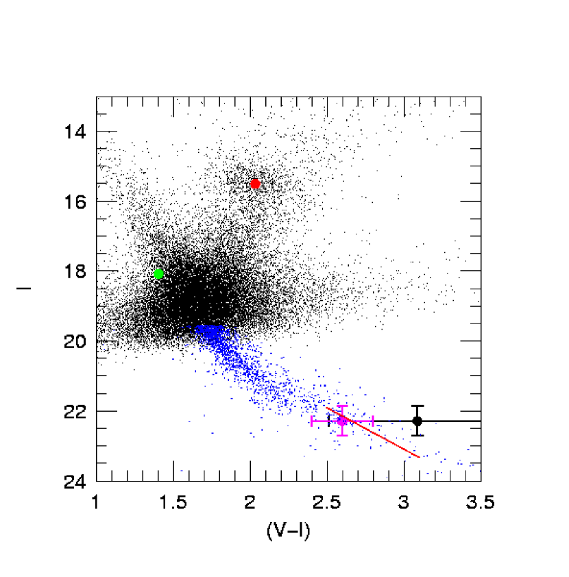
Figure 2: CMD of the OGLE-2004-BLG-343 field. Hipparcos main-sequence stars (blue dots), placed at $10^{-0.15/5}R_{0}=7.5\,$kpc and reddened by the reddening vector derived from the clump, are displayed with the OGLE-II stars (black dots). The Reid (1991) relation is plotted by the red solid line over the Hipparcos stars. On the CMD, the magenta filled circle is the red clump and the green filled circle is the blended star. The large black filled circle is the OGLE $V$ measurement of the source with of $1\sigma$ error bars, which sets a lower limit for the source $V-I$ color. The magenta filled circle with error bars is the result of combining the $(I-H)/(V-I)$ information (see Fig. 3) with the OGLE measurement.

As discussed in § 2, however, $V$-band measurements were begun only when the source had fallen nearly to baseline. Hence, the measurement of the $(V-I)$ color obtained by this standard procedure has very large errors and indeed is consistent with infinitely red ($F_{{\rm s},V}=0$) at the $2\,\sigma$ level (see Fig. 2). The CMD itself is based on OGLE-II photometry, and we have therefore shifted the OGLE-III-derived fluxes by $\Delta I=I_{\rm OGLE-II}-I_{\rm OGLE-III}=0.26$ mag. On this now calibrated CMD, the clump is at $(I,V-I)_{\rm clump}=(15.51,2.04)$. Hence, the dereddened source color and magnitude are given by $(I,V-I)_{0}=(I,V-I)+(I,V-I)_{0,\rm clump}-(I,V-I)_{\rm clump}=(I,V-I)-(1.34,1.04)$, the final offset being the reddening vector. This vector corresponds to $R_{VI}=1+1.34/1.04=2.29$, which is somewhat high compared to values obtained by Sumi (2004) for typical bulge fields. However, we will present below independent evidence for this or a slightly higher value of $R_{VI}$. Figure 2 also shows the position of the blended light, which lies in the so-called reddening sequence of foreground disk main sequence stars. This raises the question as to whether this blended star is actually the lens. We return to this question in § 5.

The source star is substantially fainter than any of the other stars in the OGLE-II CMD. In order to give a sense of the relation between this source CMD position and those of main-sequence bulge stars, we also display the Hipparcos main sequence (ESA, 1997), placed at $10^{-0.15/5}R_{0}=7.5\,$kpc and reddened by the reddening vector derived from the clump. At the best-fit value, $V-I=3.09$, the source lies well in front of (or to the red of) the bulge main-sequence. However, given the large color error, it is consistent with lying on the bulge main sequence at the $1\,\sigma$ level.

To obtain additional constraints on the color, we consider the $\mu$FUN instrumental $H$-band data. The single highly-magnified $(A\sim 40)$ $H$-band point (together with a few baseline points) yields $I_{\rm OGLE-II}-H_{\rm{\mu}FUN}=0.59\pm 0.11$ source color. To be of use, this must be translated to a $(V-I)_{\rm OGLE-II}$ color using a $(V-I)/(I-H)$ color-color diagram of the stars in the field.

Unfortunately, there are actually very few field stars in the appropriate color range. This partly results from the small size ($\sim 2$ arcmin²) of the $H$-band image and partly from the fact that a large fraction of stars are either too faint to measure in $V$-band or saturated in $H$-band. We therefore calibrate the $\mu$FUN $H$-band data by aligning them to Two Micron All Sky Survery (2MASS) data and generate a $(V-I)/(I-H_{\rm 2MASS})$ color-color diagram by matching stars from the 2MASS $H$-band data with OGLE-II $V,I$ photometry in a larger field centered on OGLE-2004-BLG-343. We find that $(H_{\rm 2MASS}-H_{\rm\mu{FUN}})=-1.99\pm 0.01$ from 48 stars in common in the field, with a scatter of 0.08 mag. We transform the above $I-H_{\rm{\mu}FUN}$ color to $I-H_{\rm 2MASS}$ and plot it as a vertical line on a $(V-I)/(I-H_{\rm 2MASS})$ color-color diagram (see Fig. 3). From the intersection of the vertical line with the diagonal track of stars in the field, we infer $V-I=2.40\pm 0.15$.

Since the field stars used to make the alignment are giants, this transformation would be strictly valid only if the source were a giant as well. However, the source star is certainly a dwarf (see Fig. 2). After transforming 2MASS to standard infrared bands (Carpenter, 2001), we use the data from Tables II and III of Bessell & Brett (1988) to construct dwarf and giant tracks on a $(V-I)_{0}/(I-H)_{0}$ color-color diagram. These are approximately coincident for blue stars $(I-H)_{0}<1.6$ but rapidly separate by 0.28 mag in $(V-I)_{0}$ by $(I-H)_{0}=1.7$. In principle, we should just adjust our estimate $(V-I)$ by the difference between these two tracks at the dereddened $(I-H)_{0}$ color of the source. Unfortunately, there are two problems with this seemingly straightforward procedure. First, the Bessell & Brett (1988) giant track displays a modest deviation from its generally smooth behavior close to the color of our source, a deviation that is not duplicated by either the giants in our field or the color-color diagram formed by combining Hipparcos and 2MASS data, which both show the same smooth behavior at this location. Second, if the Hipparcos/2MASS diagram or the Bessell & Brett (1988) diagram is reddened using the selective and total extinctions determined above from the position of the clump, then the giant tracks do not align with our field giants. To obtain alignment, one must use $R_{VI}=2.4$. The conflict among these three determinations of $R_{VI}$ ($1.9$–$2.1$ [Sumi 2004], 2.29 [clump], $\sim 2.4$ [Gould et al. 2001]) is quite a puzzle, but not one that we can explore here.

The bottom line is that there is considerable uncertainty in the dwarf-minus-giant adjustment but only in the upward direction. To take account of this, we add 0.2 mag error in quadrature to the upward error bar and finally adopt $V-I=2.4^{+0.25}_{-0.15}$ for the indirect color determination via the $(I-H)$ measurement. Finally, we combine this with the direct measurement of $V-I=3.09$ based on the combined $V$ and $I$ light curve. Because the errors on the latter measurement are extremely large (and are Gaussian in flux rather than magnitudes), we determine the probability distribution for the combined determination numerically in a flux-based calculation and then convert to magnitudes. We finally find $V-I=(V-I)_{\rm best}\pm\sigma{(V-I)}=2.60\pm 0.20$, which we show as a magenta point in Figure 2. Hence,

$$(V-I)_{0}=1.56\pm 0.20.$$ (4)

In contrast to most microlensing events that have been analyzed for planets, the color of OGLE-2004-BLG-343 is fairly uncertain. The color enters the analysis in two ways. First, it indicates the surface brightness and so determines the relation between dereddened source flux and angular size. Second, it determines the limb-darkening coefficient.

Given the color error, we consider a range of colors in our analysis and integrate over this range, just as we integrate over a range of impact parameters $u_{0}$ and source sizes (normalized to $\theta_{\rm E}$) $\rho_{*}$. We allow colors over the range $2.2<(V-I)<3.0$ corresponding to $1.16<(V-I)_{0}<1.96$. We integrate in steps of 0.1 mag. For each color, we adopt a surface brightness such that the source size $\theta_{*}$ is given by

$$\theta_{*}=\theta_{(V-I)}\,10^{-0.2(I-I_{\rm best})},$$ (5)

where $I$ is the (reddened) apparent magnitude in the model, $I_{\rm best}=22.24$, and $\theta_{2.2}\ldots\theta_{3.0}=(0.350,0.371,0.391,0.421,0.466,0.515,0.546,0.580,0.615)\mu$as. These values are derived from the color/surface-brightness relations for dwarf stars given in Kervella et al. (2004) using the method as described in Yoo et al. (2004a). In our actual calculations, we use the full distribution of source radii, but for reference we note that the $1\sigma$ range of this quantity is

$$\theta_{*}=0.47\pm 0.13\mu{\rm as}.$$ (6)

We find from the models of Claret (2000) and Hauschildt et al. (1999) that the linear limb-darkening coefficients for dwarfs in our adopted color range vary by only a few hundredths. Therefore, for simplicity, we adopt the mean of these values

$$\Gamma_{I}=0.50$$ (7)

for all colors. This corresponds to $c=3\Gamma/(2+\Gamma)=0.60$ in the standard limb-darkening parameterization (Afonso et al., 2000).

Finally, each model specifies not only a color and magnitude for the source, but also a source distance. Evaluation of the likelihood of each specific combination of these requires a color-magnitude relation. We adopt (Reid, 1991)

$$M_{I}=2.37(V-I)_{0}+2.89$$ (8)

with a scatter of 0.6 mag. The ridge of this relation is shown as a red line segment in Figure 2, with the sources placed at $10^{-0.15/5}R_{0}=7.5\,$kpc and reddened according to the red-clump determination, just as was done for the Hipparcos stars. This track is in reasonable agreement with the Hipparcos stars.

3.3 Finite-Source Effects

Yoo et al. (2004b) define $z_{0}\equiv u_{0}/\rho_{*}$ (where $\rho_{*}=\theta_{*}/\theta_{\rm E}$ is the angular size of the source $\theta_{*}$ in units of $\theta_{\rm E}$), which is a useful parameter to characterize the finite-source effects in single-lens microlensing events. We fit the observational data to a set of point-lens models on a grid of ($u_{0}$, $z_{0}$) and then compare the resulting $\chi^{2}$ with the best-fit PSPL model. As mentioned in § 3.2, we adopt the limb-darkening formalism of Yoo et al. (2004b) and for simplicity choose $\Gamma_{I}=0.50$.

Figure 4 displays the resulting $\Delta\chi^{2}$ contours. It shows that the 1 $\sigma$ contour extends from $z_{0}\simeq 0.2$ to arbitrarily large $z_{0}$. This is qualitatively similar to OGLE-2003-BLG-423 as analyzed in Yoo et al. (2004b). However, as we demonstrate in § 3.4, the range of $z_{0}$ that is consistent with the Galactic model is quite different for these two events. This is to be expected since $z_{0}=u_{0}/\rho_{*}=(u_{0}/\theta_{*})\theta_{{\rm E}}$, and $u_{0}/\theta_{*}$ is roughly 8 times smaller for this event, while $\theta_{{\rm E}}$ is generally of the same order.

Figure 4 shows contours for both $A_{\rm max}$ and $u_{0}^{-1}$. For $z_{0}\equiv u_{0}/\rho_{*}>2$, these are very similar, which is expected because in the absence of finite-source effects (and for $u_{0}\ll 1$), $A_{\rm max}=u_{0}^{-1}$. Note that the $A_{\rm max}$ contours are roughly rectangular, so that while $z_{0}$ is not well constrained, the $3\sigma$ lower limit $A_{\rm max}>10^{3.16}\sim 1450$ is quite well defined. This shows that although the blending is very severe, it is also very well constrained, implying that the event’s high magnification is secure.

3.4 Monte-Carlo Simulation

We perform a similar Monte-Carlo simulation using a Han & Gould (1996, 2003) model as described in Yoo et al. (2004b) by taking into account all combinations of source and lens distances, $D_{\rm l}<D_{\rm s}$, uniformly sampled along the line of sight toward the source $(l,b)=(4.21,-3.47)$. The simulation adopts the Gould (2000) mass function taking into account the bulge main sequence stars, white dwarfs (distributed around $0.6{\rm\ M_{\odot}}$), neutron stars (narrowly peaked at $1.35{\rm\ M_{\odot}}$), and stellar-mass black holes. This mass function is adequate to describe mass distributions of disk lenses except that the disk contains stars with masses greater than $1{\rm\ M_{\odot}}$ while the bulge does not. However, a disk main sequence star more massive than the Sun will be too bright to be the lens star for this event (see Fig. 2); so for simplicity, we use this mass function for both disk and bulge in our simulation. In Yoo et al. (2004b), the source flux is determined from the $t_{\rm E}$ for each Monte-Carlo event since only the PSPL model is considered at this step. However, when finite-source effects are taken into account, each $t_{\rm E}$ corresponds to a series of $F_{\rm s}$ depending on the source size $\rho_{*}$, so there is no longer a 1-1 correspondence between $F_{\rm s}$ and $t_{\rm E}$. As discussed in Yoo et al. (2004a), $\theta_{*}$ can be deduced from the source’s dereddened color and magnitude. Since $\theta_{\rm E}$ is known for each simulated event, $\rho_{*}$ is a direct function of $F_{\rm s}$ and the $(V-I)$ color of the source,

$$\rho_{*}={\theta_{(V-I)}\over\theta_{\rm E}}\,\sqrt{F_{\rm s}\over F_{\rm best}},$$ (9)

where $F_{\rm best}$ corresponds to $I_{\rm best}$ in equation (5). Using this constraint, we fit the $k$-th Monte-Carlo event to a point-lens model with finite-source effects, holding $t_{{\rm E},k}$ fixed at the value given by the simulation, for a variety of $(V-I)$ color values inferred from § 3.2. Hence, for the $j$-th $(V-I)$ color and $k$-th Monte-Carlo event, we have best-fit single-lens light-curve parameters $t_{0,j,k}$, $u_{0,j,k}$, $\rho_{*,j,k}$, $F_{{\rm s},j,k}$, $F_{{\rm b},j,k}$, as well as $\Delta\chi^{2}_{j,k}\equiv\chi^{2}_{j,k}-\chi^{2}_{\rm PSPL}$. We construct a three-dimensional table that includes these six quantities as well as the other parameters from the Monte-Carlo simulation ($t_{{\rm E},k}$, $\theta_{{\rm E},k}$, ${D_{{\rm s},k}}$, ${D_{{\rm l},k}}$, ${M_{{\rm l},k}}$, $\Gamma_{k}$), the Einstein timescale and radius, the source and lens distances, the lens mass, and the event rate. From these can also be derived two other important quantities, the source absolute magnitude $M_{I,j,k}$ and the physical Einstein radius $r_{{\rm E},k}\equiv{\theta_{{\rm E},k}\times{D_{{\rm l},k}}}$. This three-dimensional table is composed of nine two-dimensional tables, one for each $(V-I)_{j}$ color. Each table contains approximately 200,000 rows, one for each simulated event. To make the notation more compact, we refer to the parameters $a,b,c,...$ lying in the bin $a\in[a_{{\rm min}},a_{{\rm max}}];b\in[b_{{\rm min}},b_{{\rm max}}];c\in[c_{{\rm min}},c_{{\rm max}}]...$ as ${\rm bin}(\{a,b,c,...\})$.

Similarly to Yoo et al. (2004b), the posterior probability of $a_{i}$ lying in ${\rm bin}(a_{i})$ is given by

$$P[{\rm bin}(a_{i})]\propto\sum_{j,k}{{(P_{V-I})_{j}}\times(P_{\rm Reid})_{j,k}\times\exp[-\Delta\chi_{j,k}^{2}/2]\times{\rm BC}[{\rm bin}({\{a_{i}\}}_{j,k})]}\times\Gamma_{k},$$ (10)

where $(P_{\rm Reid})_{j,k}=\exp(-\{(M_{I})_{j,k}-M_{I,\rm Reid}[(V-I)_{0,j}]\}^{2}/2[\sigma^{2}_{\rm Reid}+{(\sigma_{M_{I}})}^{2}_{j,k}])$ accounts for the scatter ($\sigma_{\rm Reid}=0.6$) in $M_{I}$ about the Reid relation plus the dispersion ${(\sigma_{M_{I}})}_{j,k}$ from light-curve fitting, $(P_{V-I})_{j}=\exp\{-[(V-I)_{j}-(V-I)_{\rm best}]^{2}/2\sigma^{2}_{(V-I)}\}$ reflects the uncertainty in $V-I$ color, and ${\rm BC}$ is a boxcar function defined by ${\rm BC}[{\rm bin}(a)]\equiv\Theta\left(a-a_{{\rm min}}\right)\times\Theta\left(a_{{\rm max}}-a\right)$.

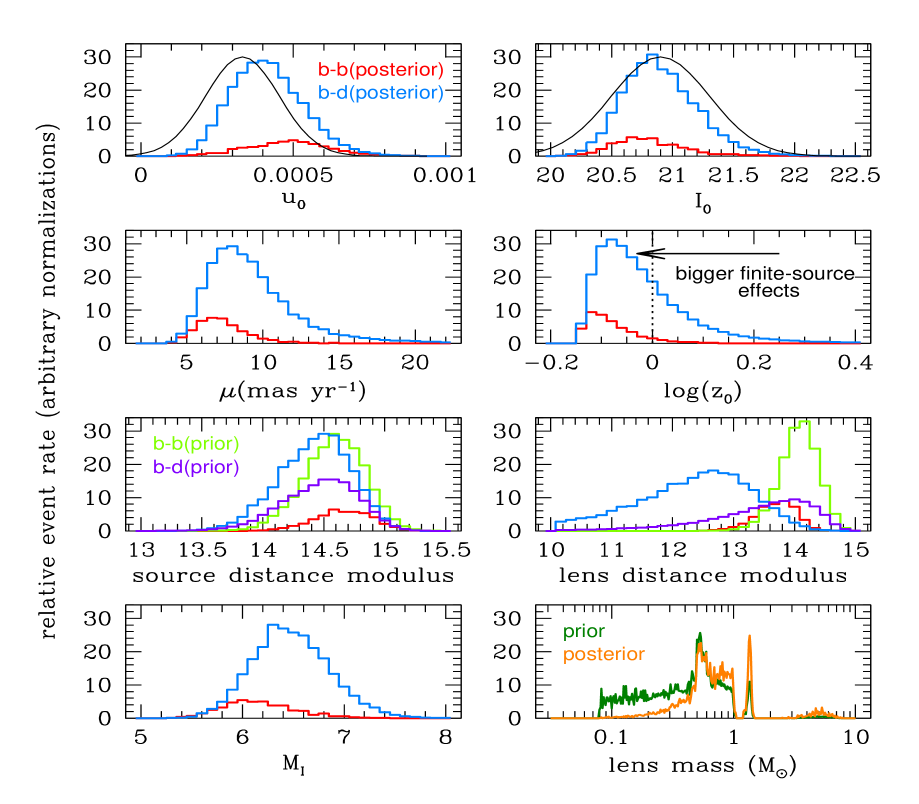
Figure 5: Probability distributions of $u_{0}$, dereddened apparent $I$-band magnitude of the source $I_{0}$, proper motion $\mu$, $\log(z_{0})$, source distance modulus, lens distance modulus, absolute $I$-band magnitude of the source $M_{I}$, and lens mass for Monte Carlo events toward the line of sight of OGLE-2004-BLG-343. Blue histograms represent the posterior probability distributions for bulge-disk microlensing events while red ones represent the posterior probability distributions for bulge-bulge events. In the source and lens distance-modulus panels, histograms in purple and green represent the prior probability distributions for bulge-disk and bulge-bulge events, respectively. The black Gaussian curves in the $u_{0}$ and $I_{0}$ panels show probability distributions from PSPL light-curve fitting alone. In the lens mass panel, the dark green histogram shows the prior probability distribution, while the orange histogram represents the posterior distribution.

Figure 5 shows the posterior probability distributions of various parameters, including $u_{0}$, dereddened apparent $I$-band magnitude of the source $I_{0}$, proper motion $\mu$, $z_{0}$, source distance modulus, lens distance modulus, absolute $I$-band magnitude of the source $M_{I}$, and lens mass. The blue and red histograms represent bulge-disk events and bulge-bulge events, respectively. The relative event rate is normalized in the same way for both bulge-disk and bulge-bulge events. The total rate for bulge-disk events is about $6$ times larger than that for bulge-bulge events, which means that the Monte-Carlo simulation tends strongly to favor bulge-disk events.

The Einstein radii are on average smaller for bulge-bulge events than for bulge-disk events, and as a result, the bulge-bulge events tend to have bigger $\rho_{*}$ and hence smaller $z_{0}$. However, the top right panel of Figure 5 shows that the $z_{0}$ probability distributions have similar shapes for both bulge-bulge and bulge-disk events. This is because the (lack of) finite-source effects constrain $z_{0}\gtrsim 0.7$ at the $3\sigma$ level (see Fig. 4), which cuts off the lower end of the $z_{0}$ distributions for both categories of events. Since bulge-disk events have smaller $\rho_{*}$ than bulge-bulge events, the $u_{0}$ posterior probability distribution peaks at a lower value for the former. Furthermore, since $z_{0}\gtrsim 0.7$, the proper motion is constrained to be $\mu={\theta_{*}z_{0}/t_{{\rm eff}}}\gtrsim 7{\rm mas/yr}$, which is typical of bulge-disk events but $\gtrsim 2$ times the proper motion of typical bulge-bulge events.

Figure 5 also shows the distributions of $u_{0}$ and $I_{0}$ from the light-curve data alone by a black solid line. In strong contrast to the corresponding diagrams for OGLE-2003-BLG-423 presented by Yoo et al. (2004b), the light-curve based parameters agree quite well with the Monte-Carlo predictions. In the source distance-modulus panel, the prior distributions for bulge-disk and bulge-bulge events are shown in purple and green histograms, respectively. Again, distinct from OGLE-2003-BLG-423, the most likely source distances of this event agree reasonably well with typical values from the prior distributions. Moreover, from Figure 5, the peak values of source $M_{I}$ distributions are also in good agreement with those derived from the Reid relation ($M_{I}=6.59$ for $\left[V-I\right]_{0}=1.56$, see eq. [8]). Therefore, the source of this event shows very typical characteristics as represented by the Monte-Carlo simulation. Also unlike OGLE-2003-BLG-423, the probability that $z_{0}\lesssim 1$ is very high for both bulge-disk and bulge-bulge events. Therefore, finite-source effects must be taken into account in the analysis of this event. In addition to the posterior probability distribution (orange) of the lens mass, the prior distribution (dark green) is displayed in Figure 5 as well. In microlensing analyses, the lens mass is commonly assigned a “typical” value (for example, $0.3{\rm\ M_{\odot}}$). However, Figure 5 shows that, lenses with relatively high mass are strongly favored for this event as compared to the prior distribution. Detailed discussions on the lens properties are presented in § 5.

4 Detecting Planets

While there are no obvious deviations from point-lens behavior in the light curve of OGLE-2004-BLG-343 at our adopted threshold of $\Delta\chi^{2}_{\rm min}=60$, planetary deviations might be difficult to recognize by eye. We must therefore conduct a systematic search for such deviations. Logically, this search should precede the second step of testing to determine what planets we could have detected had they been there. However, as a practical matter it makes more sense to first determine the range of parameter space for which we are sensitive to planets because it is only this range that needs to be searched for planets. We therefore begin with this detection efficiency calculation.

4.1 Detection Efficiency

As reviewed in § 1.2, a variety of methods have been proposed to calculate the planetary sensitivities of microlensing events, either in predicting planetary detection efficiencies theoretically or in analyzing real observational data sets. In those methods, $\Delta{\chi^{2}}$ is often calculated by subtracting the $\chi^{2}$ of single-lens models from that of the binary-lens models to evaluate detection sensitivities. However, the ways in which single-lens and binary-lens models are compared differ from study to study. As noted by Griest & Safizadeh (1998) and Gaudi & Sackett (2000), for real planetary light curves, the lens parameters are not known a priori. Therefore, $\Delta{\chi^{2}}$ will generally be exaggerated if one subtracts from the binary lens model the single-lens model that has the same $t_{0}$, $u_{0}$, and $t_{\rm E}$ instead of the best-fit single-lens model to the binary light curve. One important factor contributing to this exaggeration is that the center of the magnification pattern (referred to as the center of the caustic in Yoo et al. 2004b) in the binary-lens case is no longer the position of the primary star as it is in the single-lens model (Dominik, 1999b; An & Han, 2002). Therefore light-curve parameters such as $u_{0}$ and $t_{0}$ will shift correspondingly. We find that by not taking into account this effect and directly comparing the simulated binary (i.e., planetary) light curve with the best-fit single-lens model to the data, Abe et al. (2004) exaggerate the planetary sensitivity of MOA 2003-BLG-32/OGLE 2003-BLG-219, although it remains the most sensitive event analyzed to date (see Appendix B).

Following Gaudi & Sackett (2000), planetary systems are characterized by a planet-star mass ratio $q$, planet-star separation in Einstein radius $b$, and the angle $\alpha$ of the source trajectory relative to the planet-star axis. In our binary-lens calculations, $u_{0}$ and $t_{0}$ are defined with respect to the center of magnification discussed above. According to Gaudi & Sackett (2000), the next step is to fit the data to both PSPL models and binary-lens models with a variety of $(b,q,\alpha)$ and calculate $\Delta{\chi^{2}{(b,q,\alpha)}}=\chi^{2}{(b,q,\alpha)}-\chi^{2}_{\rm PSPL}$. Then $\Delta{\chi^{2}{(b,q,\alpha)}}$ is compared with a threshold value $\chi^{2}_{\rm thres}$: if $\Delta{\chi^{2}}>\chi^{2}_{\rm thres}$ then a planet with parameters $b$, $q$, and $\alpha$ is claimed to be excluded while it is detected if $\Delta{\chi^{2}}<-\chi^{2}_{\rm thres}$. The $(b,q)$ detection efficiency is then obtained by integrating $\Theta(\Delta{\chi^{2}}-\Delta{\chi_{\rm thres}^{2}})$ over $\alpha$ in the exclusion region at fixed $(b,q)$, where $\Theta$ is a step function. However, Gaudi et al. (2002) point out that for events with poorly constrained light-curve parameters, which is the case for OGLE-2004-BLG-343, this method will significantly underestimate the sensitivities since the binary-lens models will minimize the $\chi^{2}$ over the relatively large available parameter space. As discussed in Yoo et al. (2004b), the detection efficiency should be evaluated at a series of allowed $u_{0}$ values. To take finite-source effects into account, we generate a grid of permitted $(u_{0},\rho_{*})$, and each $(u_{0,m},\rho_{*,m})$ bin is associated with the probability $P[{\rm bin}(\{u_{0,m},\,\rho_{*,m}\})]$ obtained using the following equation:

$$P[{\rm bin}(\{u_{0,m},\,\rho_{*,m}\})]\propto\sum_{j,k}{P_{m,j,k}}$$ (11)

where

$${P_{m,j,k}={(P_{V-I})_{j}}\times(P_{\rm Reid})_{j,k}\times\exp[-\Delta\chi_{j,k}^{2}/2]\times{\rm BC}[{\rm bin}(\{u_{0,m}\}_{j,k})]\times{\rm BC}[{\rm bin}(\{\rho_{*,m}\}_{j,k})]}\times\Gamma_{k}$$ (12)

If the light-curve parameters were well-constrained, the approaches of Gaudi & Sackett (2000) and Rhie et al. (2000) would be very nearly equivalent, with the former retaining a modest philosophical advantage, since it uses only the observed light curve and does not require construction of light curves for hypothetical events. However, because in our case these parameters are not well constrained, the Gaudi & Sackett (2000) approach would require integration over all binary-lens parameters (except $F_{\rm s}$ and $F_{\rm b}$). Regardless of its possible philosophical advantages, this approach is therefore computationally prohibitive in the present case. We therefore do not follow Gaudi & Sackett (2000), but instead construct a binary light curve with the same observational time sequence and photometric errors as the OGLE observations of OGLE-2004-BLG-343, for each $(b,q,\alpha\,;u_{0},\rho_{*})$ combination and the associated probability-weighted parameters $\mbox{\boldmath$a$}_{{\rm lc}}$: $t_{0}$, $t_{\rm E}$, $F_{\rm s}$ and $F_{\rm b}$ in the $m$-th $(u_{0},\rho_{*})$ bin,

$${\mbox{\boldmath$a$}_{\rm lc(weighted),m}}={{\sum_{j,k}\limits{P_{m,j,k}{{\mbox{\boldmath$a$}_{{\rm lc},j,k}}}}\over{\sum_{{j,k}}\limits{P_{m,j,k}}}}}.$$ (13)

Then each simulated binary light curve $(b,q,\alpha\,;u_{0,m},\rho_{*,m})$ is fitted to a single-lens model with finite-source effects whose best fit yields $\chi^{2}(b,q,\alpha\,;u_{0,m},\rho_{*,m})$. Another set of artificial binary light curves is generated under the assumption that OGLE had triggered a dense series of observations following the internal alert at HJD^′ 3175.54508. These cover the peak of the event with the normal OGLE frequency and are used to compare results with those obtained from the real observations.

Magnification calculations for a binary lens with finite-source effects are very time-consuming. Besides $(b,q,\alpha)$, our calculations are also performed on $(u_{0},\rho_{*})$ grids, two more dimensions than in any previous search of a grid of models with finite-source effects included. This makes our computations extremely expensive, comparable to those of Gaudi et al. (2002), which equaled several years of processor time. Therefore, we have developed two new binary-lens finite-source algorithms to perform the calculations, as discussed in detail in Appendix A.

In principle, we should consider the full range of $b$, i.e., $0<b<\infty$; in practice, it is not necessary to directly simulate $b<1$ due to the famous $b\leftrightarrow b^{-1}$ degeneracy (Dominik, 1999a; An, 2005). Instead, we just map the $b>1$ results onto $b<1$ except for the isolated sensitive zones along the $x-$axis caused by planetary caustics perturbations.

We define the planetary detection efficiency $\epsilon(b,q)$ as the probability that an event with the same characteristics as OGLE-2004-BLG-343, except that the lens is a planetary system with configuration of $(b,q)$, is inconsistent with the single-lens model (and hence would have been detected),

$$\epsilon(b,q,\alpha) = \{\sum_{m}\limits\Theta\left[\chi^{2}(b,q,\alpha\,;u_{0,m},\rho_{*,m})-\Delta\chi^{2}_{\rm thres}\right]$$ (14)

$$\times P[{\rm bin}(\{u_{0,m},\,\rho_{*,m}\})]\}$$

$$\times\{\sum_{m}\limits P[{\rm bin}(\{u_{0,m},\,\rho_{*,m}\})]\}^{-1}$$

and

$$\epsilon(b,q)={1\over 2\pi}\int_{0}^{2\pi}{\epsilon(b,q,\alpha)}d\alpha.$$ (15)

4.2 Constraints on Planets

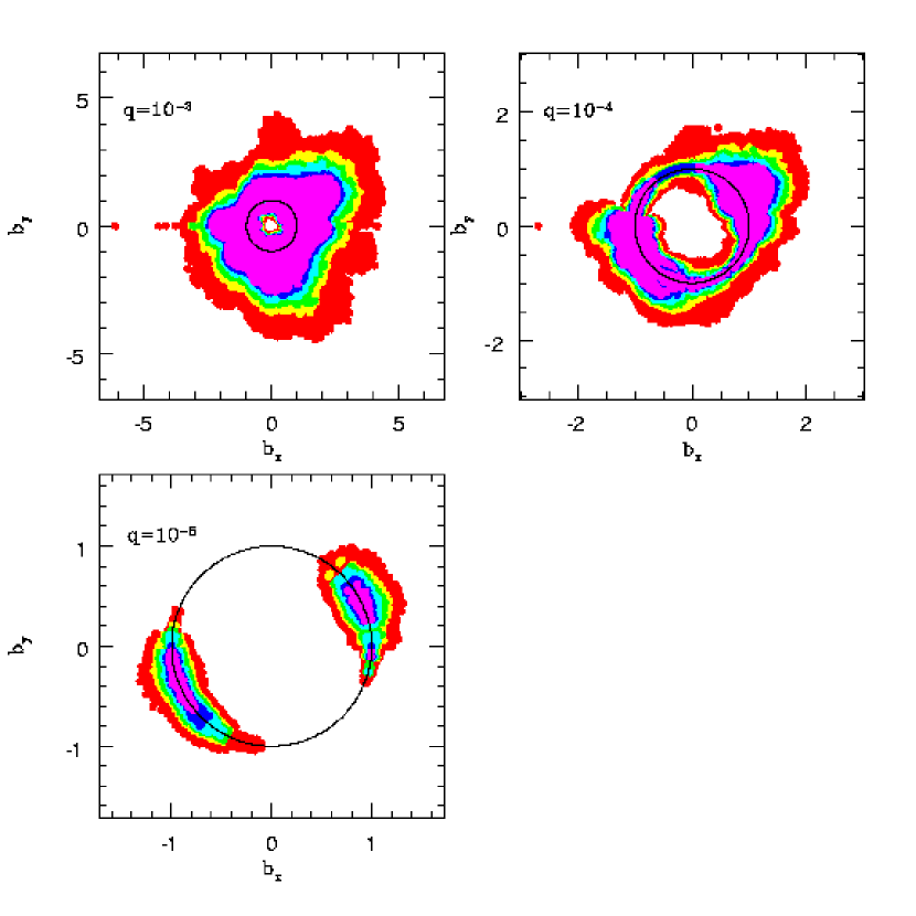
Figure 6: (For real data) Planetary detection efficiency for mass ratios $q=10^{-3}$, $10^{-4}$, and $10^{-5}$ for OGLE-2004-BLG-343 as a function of the planet-star separation $b_{x}=b\times{\cos{\alpha}}$ and $b_{y}=b\times{\sin{\alpha}}$ in the units of ${\theta}_{\rm E}$ where $\alpha$ is the angle of planet-star axis relative to the source-lens direction of motion. Different colors indicate 10% (red), 25% (yellow), 50% (green), 75% (cyan), 90% (blue) and 100% (magenta) efficiency. The black circle is the Einstein ring, i.e., $b=1$.

Figure 6 shows the planetary detection efficiency of OGLE-2004-BLG-343 for planets with mass ratios $q=10^{-3}$, $10^{-4}$, and $10^{-5}$, as a function of $b$, the planet-star separation (normalized to $\theta_{\rm E}$), and $\alpha$, the angle that the moving source makes with the binary axis passing the primary lens star on its left. Different colors indicate 10%, 25%, 50%, 75%, 90% and 100% efficiency. Note that the contours are elongated along an axis that is roughly $60^{\circ}$ from the vertical (i.e., the direction of the impact parameter for $\alpha=0$). This reflects the fact that the point closest to the peak occurs at $t=2453175.77626$ when $(t-t_{0})/t_{\rm E}=2.16u_{0}$, and so when the source-lens separation is at an angle $\tan^{-1}2.16=65^{\circ}$. For $q=10^{-3}$, the region of 100% efficiency extends through $360^{\circ}$ within about one octave on either side of the Einstein ring. However, at lower mass ratios there is 100% efficiency only in restricted areas close to the Einstein ring and along the above-mentioned principal axis.

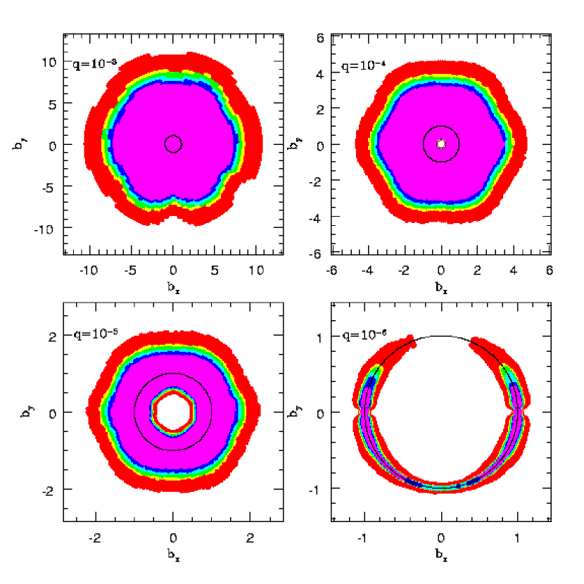
Figure 8: (For fake data) Planetary detection efficiency for mass ratios $q=10^{-3}$, $10^{-4}$, $10^{-5}$ and $10^{-6}$ of OGLE-2004-BLG-343 augmented by simulated data points covering the peak as a function of the planet-star separation $b_{x}$ and $b_{y}$ in the units of ${\theta}_{\rm E}$. Different colors indicate 10% (red), 25% (yellow), 50% (green), 75% (cyan), 90% (blue) and 100% (magenta) efficiency. The black circle is the Einstein ring, i.e., $b=1$.

Figure 7 summarizes an ensemble of all figures similar to Figure 6, but with $q$ ranging from $10^{-2.5}$ to $10^{-5.0}$ in 0.1 increments. To place this summary in a single figure, we integrate over all angles $\alpha$ at fixed $b$. Comparison of this figure to Figure 8 from Gaudi et al. (2002) shows that the detection efficiency of OGLE-2004-BLG-343 is similar to that of MACHO-1998-BLG-35 and OGLE-1999-BUL-35 despite the fact that their maximum magnifications are $A_{\rm max}\sim 100$, roughly 30 times lower than OGLE-2004-BLG-343. Of course, part of the reason is that OGLE-2004-BLG-343 did not actually probe as close as $u=u_{0}\sim 1/3000$ because no observations were taken near the peak. However, observations were made at $u\sim 1/1200$, about 12 times closer than in either of the two events analyzed by Gaudi et al. (2002). One problem is that because the peak was not well covered, there are planet locations that do not give rise to observed perturbations at all. But this fact only accounts for the anisotropies seen in Figure 6. More fundamentally, even perturbations that do occur in the regions that are sampled by the data can often be fitted to a point-lens light curve by “adjusting” the portions of the light curve that are not sampled.

Note the central “spike” of reduced detection efficiency plots near $b=1$. As first pointed out by Bennett & Rhie (1996), this is due to the extreme weakness of the caustic for nearly resonant ($b\sim 1$) small mass-ratio ($q\ll 1$) binary lenses.

4.3 No Planet Detected

Based on the detection efficiency levels we obtained in § 4.2, we fit the observational data to binary-lens models to search for a planetary signal in the regions with efficiency greater than zero from $q=10^{-5}$ to $q=10^{-2.5}$. We find no binary-lens models satisfying our detection criteria. In fact, the total $\chi^{2}$ contributions to the best-fit single-lens model of the observational points over the peak ( HJD $=2453175.5-2453176.0$) are no more than 30, so even if all of these deviations were due to a planetary perturbation, such a binary-lens solution would not easily satisfy our $\Delta{\chi^{2}}=60$ detection criteria. Therefore there are no planet detections in OGLE-2004-BLG-343 data.

4.4 Fake Data

Partly to explore further the issue of imperfect coverage of the peak, and partly to understand how well present microlensing experiments can probe for planets, we now ask what would have been the detection efficiency of OGLE-2004-BLG-343 if the internal alert issued on HJD^′ 3175.54508 had been acted upon.

Of course, since the peak was not covered, we do not know exactly what $u_{0}$ and $\rho$ for this event are. However, for purposes of this exercise, we assume that they are near the best fit as determined from a combination of the light-curve fitting and the Galactic Monte Carlo, and for simplicity, we choose $u_{0}=0.00040,\rho_{*}=0.00040$ which is very close to the best-fit combination. We then form a fake light curve sampled at intervals of 4.3 minutes, starting from the alert and continuing to the end of the actual observations that night. This sampling reflects the intense rate of OGLE follow-up observations actually achieved during this event (see § 2). We assume errors similar to those of the actual OGLE data at similar magnifications. For those points that are brighter than the brightest OGLE point, the minimum actual photometric errors are assigned. We also assume that the color information is known exactly in this case to be $V-I=2.6$. We then analyze these fake data in exactly the same way that we analyze the real data. In contrast to the real data, however, we do not find a finite range of $z_{0}\equiv u_{0}/\rho_{*}$ that are consistent with the fake data. Rather, we find that all consistent parameter combinations have $z_{0}=1$ almost identically. We therefore consider only a one-dimensional set of $(u_{0},\rho_{*})$ combinations subject to this constraint.

Figure 8 is analogous to Figure 6 except that the panels show planet sensitivities for $q=10^{-3}$, $10^{-4}$, $10^{-5}$, and $10^{-6}$, that is, an extra decade. In sharp contrast to the real data, these sensitivities are basically symmetric in $\alpha$, except for the lowest value of $q$. Sensitivities at all mass ratios are dramatically improved. For example, at $q=10^{-3}$, there is 100% detection efficiency over 1.7 dex in $b$ ($1/7\lesssim b\lesssim 7$). Even at $q=10^{-5}$ (corresponding to an Earth-mass planet around an M star), there is 100% efficiency over an octave about the Einstein radius.

Figure 9 is the fake-data analog of Figure 7. It shows that this event would have been sensitive to extremely low mass-ratios, lower than those accessible to any other technique other than pulsar timing.

4.5 Detection Efficiency in Physical Parameter Space

One of the advantages of the Monte Carlo approach of Yoo et al. (2004b) is that it permits one to evaluate the planetary detection efficiency in the space of the physical parameters, planet mass and projected physical separation ($m_{p},r_{\perp}$), rather than just the microlensing parameters $(b,q)$. Figures 10 and 11 show this detection efficiency for the real and fake data, respectively. The fraction of Jupiter-mass planets that could have been detected from the actual data stream is greater than $25\%$ for $0.8{\rm AU}\lesssim{r_{\perp}}\lesssim{10{\rm AU}}$ and is greater than $90\%$ for $2{\rm AU}\lesssim{r_{\perp}}\lesssim 6{\rm AU}$. There is also marginal sensitivity to Neptune-mass planets. However, the detection efficiencies would have been significantly enhanced had the FWHM around the peak been observed, as previously discussed by Rattenbury et al. (2002). For the fake data, more than $90\%$ of Jupiter-mass planets in the range $0.7{\rm AU}\lesssim{r_{\perp}}\lesssim 20{\rm AU}$ and more than $25\%$ with $0.3{\rm AU}\lesssim{r_{\perp}}\lesssim 30{\rm AU}$ would have been detected. Indeed, some sensitivity would have extended all the way down to Earth-mass planets.

5 Luminous Lens?

Understanding the physical properties of their host stars is a major component of the study of extra-solar planets. It is especially important to know the mass and distance of the lens star for planets detected by microlensing because only then can we accurately determine the planet’s mass and physical separation from the star. Obtaining similar information for microlensing events that are unsuccessfully searched for planets enables more precise estimates of the detection efficiency. There are only two known ways to determine the mass and distance of the lens: either measure both the microlensing parallax and the angular Einstein radius (which are today possible for only a small subset of events) or directly image the lens. In most cases the lens is either entirely invisible or is lost in the much brighter light of the source.

A simple argument suggests, however, that in extremely high-magnification events like OGLE-2004-BLG-343, the lens will often be easily visible and, indeed, it is the lens that is unknowingly being monitored, with the source revealing itself only in the course of the event. Events of magnification $A_{\rm max}$ require that the source be much smaller than the Einstein radius, $\theta_{*}\lesssim 2\theta_{\rm E}/A_{\rm max}$. Since $\theta_{\rm E}=\sqrt{\kappa M\pi_{\rm rel}}$, large $\theta_{\rm E}$ requires a lens that is either massive or nearby, both of which suggest that it is bright. On the other hand, a small $\theta_{*}$ implies that the source is faint. Generally, if a faint source and a bright potential lens are close on the sky, only the lens will be seen, until it starts to strongly magnify the source. This has important implications for the real time recognition of extreme magnification events, as we discuss in § 6. Here we review the evidence as to whether the blended light in OGLE-2005-BLG-343 is in fact the lens.

As was true for OGLE-2003-BLG-175/MOA-2003-BLG-45 mentioned in § 1.3, the blended light in OGLE-2004-BLG-343 lies in the “reddening sequence” of foreground disk stars. It is certainly “dazzling” by any criterion, being about 50 times brighter than the source in $I$ and 150 times brighter in $V$ (see Fig. 2). Is the blended light also due to the lens in this case?

There is one argument for this hypothesis and another against. We initiate the first by estimating the mass and distance to the blend as follows. We model the extinction due to dust at a distance $x$ along the line of sight by $dA_{I}/dx=0.4\,{\rm kpc}^{-1}e^{-qx}$ and set $q=0.26\,{\rm kpc}^{-1}$ in order to reproduce the measured extinction to the bulge $A_{I}(8\,{\rm kpc})=1.34$. Using the Reid (1991) color-magnitude relation, we then adjust the distance to the blend until it reproduces the observed color and magnitude of the blend. We find a distance modulus of 12.6 ($\sim 3.3\,{\rm kpc}$), and with the aid of the Cox (2000) mass-luminosity relation, we estimate a corresponding mass $M_{\rm l}=0.9\,{\rm\ M_{\odot}}$. Inspecting Figure 5, we see that this is almost exactly the peak of the lens-distance distribution function predicted by combining light-curve information and the Galactic model. This is quite striking because, in the absence of light-curve information, the lens would be expected to be relatively close to the source. From our Monte-Carlo simulation toward the line of sight of this event, the total prior probability of the bulge-bulge events is about 1.5 times higher than the prior probability of the bulge-disk events, and furthermore, only about $7\%$ of all events have lenses less than $3.3\,{\rm kpc}$ away (see green and purple histograms in source and lens distance modulus panels of Fig. 5). It is only because the light curve lacks obvious finite-source effects (despite its very high-magnification) that one is forced to consider lenses with large $\theta_{\rm E}$, which generally drives one toward nearby lenses in the foreground disk. Based on our experience analyzing many blended microlensing events, the blended light is most often from a bulge star rather than a disk star, which simply reflects the higher density of bulge stars. In brief, it is quite unusual for lenses to be constrained to lie in the disk, and it is quite unusual for events to be blended with foreground disk stars. This doubly unusual set of circumstances would be more easily explained if the blend were the lens.

However, if the blend were the lens, then the source and lens would be aligned to better than 1 mas during the event, and one would therefore expect that the apparent position of the source would not change as the source first brightened and then faded. In fact, we find that the apparent position does change by about $73\pm 9\,$mas. However, since the apparent source (i.e., combined source and blended light at baseline) has a near neighbor at 830 mas, which is almost as bright as the source/blend, it is quite possible that the lens actually is the blend, but that this neighbor is corrupting the astrometry.

Thus, the issue cannot be definitively settled at present. However, it could be resolved in principle by, for example, obtaining high-resolution images of the field a decade after the event when the source and lens have separated sufficiently to both be seen. If the blend is the lens, then they will be seen moving directly apart with a proper motion given $\mu=\theta_{\rm E}/t_{\rm E}$, where $\theta_{\rm E}$ is derived from the estimated mass and distance to the lens and $t_{\rm E}$ is the event timescale.

Since the blend cannot be positively identified as the lens, we report our main results using a purely probabilistic estimate of the lens parameters. However, for completeness, we also report results here based on the assumption that the lens is the blend. Compared to the previous simulation, in which we considered the full mass function and full range of distances, we sample only the narrow intervals of mass and distance that are consistent with the observed color and magnitude of the lens/blend. To implement these restrictions, we repeat the Monte Carlo, but with the additional constraint that the predicted apparent magnitudes agree with the observed blend magnitude (with an error of 0.5 mag) and that the predicted colors (using the above extinction law and the Reid 1991 color-magnitude relation) also show good agreement with the observed color (with 0.2 mag error). These errors are, of course, much larger than the observational errors. They are included to reflect the fact that the theoretical predictions for color and magnitude at a given mass are not absolutely accurate.

Figure 12 is the resulting version of Figure 10 when the Monte Carlo is constrained to reproduce the blend color and magnitude. The sensitivity contours are narrower and deeper, reflecting the fact that the diagram no longer averages over a broad range of lens masses but rather is restricted effectively to a single mass (and single distance).

6 Summary and Discussion

In this paper we present our analysis of microlensing event OGLE-2004-BLG-343, with the highest peak magnification ($A_{\rm max}=3000\pm 1100$) ever analyzed to date. The light curve is consistent with the single-lens microlensing model, and no planet has been detected in this event. We demonstrate that if the peak had been well covered by the observations, the event would have had the best sensitivity to planets to date, and it would even have had some sensitivity to Earth-mass planets (§ 4.4, § 4.5). However, this potential has not been fully realized due to human error (§ 2), and OGLE-2004-BLG-343 turns out to be no more sensitive to planets than a few other high-magnification events analyzed before (§ 4.2, § 4.5). Thus, while ground-based microlensing surveys are technically sufficient to detect very low-mass planets, the relatively short timescale of the sensitive regime of high-magnification microlensing events demands a rapidity of response that is not consistently being achieved. In the final paragraph below, we develop several suggestions to rectify this situation.

In § 3 we show that finite-source effects are important in analyzing this event, so we extend the method of Yoo et al. (2004b) to incorporate such effects in planetary detection efficiency analysis. Moreover, since magnification calculations of binary-lens models with finite-source effects are computationally remarkably expensive, and applying previous finite-source algorithms, it would have taken of order a year of CPU time to do the detection efficiency calculation required by this event. We therefore develop two new binary-lens finite-source algorithms (Appendix A) that are considerably more efficient than previous ones. The “map-making” method (Appendix A.1) is an improvement on the conventional inverse ray-shooting method, which proves to be especially efficient for use in detection efficiency calculations, while the “loop-linking” method (Appendix A.2) is more versatile and could be easily implemented in programs aimed at finding best-fit finite-source binary-lens solutions. Using these algorithms, we were able to complete the computations for this paper in about 4 processor-weeks, roughly an order of magnitude faster than would have been required using previous algorithms.

Finally, we show in § 5 that the blend, which is a Galactic disk star, might very possibly be the lens, and that this case also proves to be highly probable from the Monte-Carlo simulation. However, it seems to contradict the astrometric evidence, and we point out that this issue could in principle be solved by future high-resolution images. Among the high-magnification events discovered by current microlensing survey groups, it is very likely that the lens star, which is also the apparent source, of those events is in the Galactic disk. Thus the blended light is usually far brighter than the source, thereby increasing the difficulty in early identification of such events. This fact motivates the first of several suggestions aimed at improving the recognition of very high-magnification events:

• When events are initially alerted they should be accompanied by instrumental CMD of the surrounding field, with the location of the apparent “source” highlighted. Events whose apparent sources lie on the “reddening sequence” of foreground disk stars (see Fig. 2) have a high probability to actually be lenses of more distant (and fainter) bulge sources. These events deserve special attention even if their initial light curves appear prosaic.

• For each such event it is possible to measure the color (but not immediately the magnitude) of the source by the standard technique of obtaining two-band photometry and measuring the slope of the relative fluxes in the two bands. If the color is different from that of the apparent “source” at baseline, that will prove that this baseline light is not primarily due to the source, and it will increase the probability that this baseline object is the lens. Moreover, if the source color is relatively red, it will show that the source is probably faint and so is (1) most likely already fairly highly magnified (thereby making it possible to detect above the foreground blended light) and (2) capable, potentially at least, of being magnified to very high magnification (see § 5). This would motivate obtaining more data while the event was still faint to help predict its future behavior and would enable a guess as to how to “renormalize” the event’s apparent magnification to its true magnification. This is important because generally one cannot accurately determine this renormalization until the event is within 0.4 mag (when the event is $t_{\rm eff}$ before its peak), at which point it may well be too late to act on this knowledge.

• Both survey groups and follow-up groups should issue alerts on suspected high-magnification events guided by a relatively low threshold of confidence, recognizing that this will lead to more “false alerts” than at present. If such alerts are accompanied by a cautionary note, they will promote intergroup discussions that could lead to more rapid identification of high-magnification events without compromising the credibility of the group.

Appendix A Two New Finite-Source Algorithms

To model planetary light curves, we develop two new binary-lens finite-source algorithms. The first algorithm, called “map-making”, is the main work horse. For a fixed $(b,q)$ geometry, it can successfully evaluate the finite-source magnification of almost all data points on the light curve and can robustly identify those points for which it fails. The second algorithm, called “loop-linking”, is much less efficient than map-making but is entirely robust. We use loop-linking whenever the map-making routine decides it cannot robustly evaluate the magnification of a point. In addition, at the present time, map-making does not work for resonant lensing geometries, i.e., geometries for which the caustic has six cusps. For planetary mass ratios, resonant lensing occurs when the planet is very close to the Einstein radius, $b\sim 1$. We use loop-linking in these cases also.

A.1 Map-Making

Map-making has two components: a core function that evaluates the magnification and a set of auxiliary functions that test whether the measurement is being made accurately. If a light-curve point fails these tests, it is sent to loop-linking.

Finite-source effects are important when the source passes over or close to a caustic. Otherwise, the magnification can be evaluated using the point-source approximation, which is many orders of magnitude faster than finite-source evaluations. Hence, the main control issue is to ensure that any point that falls close to a caustic is evaluated using a finite-source algorithm or at least is tested to determine whether this is necessary. For very high magnification events, the peak points will always pass close to the central caustic. Hence, the core function of map-making is to “map” an Einstein-ring annulus in the image plane that covers essentially all of the possible images of sources that come close to the central caustic. The method must also take account of the planetary caustic(s), but we address that problem further below.

We begin by inverse ray-shooting an annulus defined by $A_{\rm PSPL}>A_{\rm min}$, where $A_{\rm PSPL}$ is the Paczyński (1986) magnification due to a point source by a point lens and $A_{\rm min}$ is a suitably chosen threshold. For OGLE-2000-BLG-343, we find that $A_{\rm min}=75$ covers the caustic-approaching points in essentially all cases. The choice of the density of the ray-shooting map is described below. Each such “shot” results in a four-element vector $(x_{i},y_{i},x_{s},y_{s})$. We divide the portion of the source plane covered by this map into a rectangular grid with $k=1,\ldots,N_{g}$ elements. We choose the size of each element to be equal to the smallest source radius being evaluated by the map. Hence, each “shot” is assigned to some definite grid element $k(x_{s},y_{s})$. We then sort the “shots” by $k$. For each light-curve point to be evaluated, we first find the grid elements that overlap the source. We then read sequentially through the sorted file from the beginning of the element’s “shots” to the end. For each “shot”, we ask whether its $(x_{s},y_{s})$ lies within the source. If so, we weight that point by the limb-darkened profile of the source at that radius. Note that a source with arbitrary shape and surface brightness profile would be done just as easily.

For each light-curve point, we first determine whether at least one of the images of the center of the source lies in the annulus. In practice, for our case, the points satisfying this condition are just those on the night of the peak, but for other events this would have to be determined on a point-by-point basis. We divide those points with images outside the annulus into two classes, depending on whether they lie inside or outside two or three rectangles that we “draw”, one around each caustic. Each rectangle is larger than the maximum extent of the caustics by a factor of $1.5$ in each direction. If the source center lies outside all of these rectangles, we assume that the point-source approximation applies and evaluate the magnification accordingly. If it lies inside one of the rectangles (and so either near or inside one of the caustics), we perform the following test to see whether the point-source approximation holds. We evaluate the point-source magnifications at five positions, namely, the source center $A(0,0)$, two positions along the source $x$-axis $A(\pm\lambda\rho_{*},0)$, and two positions along the source y-axis $A(0,\pm\lambda\rho_{*})$, where $\lambda\leq 1$ is a parameter. We demand that

$$\bigg{|}{A(\lambda\rho_{*},0)+A(-\lambda\rho_{*},0)\over 2A(0,0)}-1\bigg{|}+\bigg{|}{A(0,\lambda\rho_{*})+A(0,-\lambda\rho_{*})\over 2A(0,0)}-1\bigg{|}<4\sigma,$$ (A1)

where $\sigma$ is the maximum permitted error (defined in § A.3). We use a minimum of five values in order to ensure that the magnification pattern interior to the source is reasonably well sampled; the precise value is chosen empirically and is a compromise between computing speed and accuracy. We require the number of values to be at least $2[\rho_{*}/\sqrt{q}]$ in order to ensure that small, well-localized perturbations interior to the source caused by low mass ratio companions are not missed.

If a point passes this test, the magnification pattern in the neighborhood of the point is adequately represented by a gradient and so the point-source approximation holds. Points failing this test are sent to loop linking.

The remaining points, those with at least one image center lying in the annulus, are almost all evaluated using the sorted grid as described above. However, we must ensure that the annulus really covers all of the images. We conduct several tests to this end.

First, we demand that no more than one of the three or five images of the source center lie outside the annulus. In a binary lens, there is usually one image that is associated with the companion and that is highly demagnified. Hence, it can generally be ignored, so the fact that it falls outside the annulus does not present a problem. If more than one image center lies outside the annulus, the point is sent to loop-linking. Second, it is possible that an image of the center of the source could lie inside the annulus, but the corresponding image of another point on the source lies outside. In this case, there would be some intermediate point that lay directly on the boundary. To guard against this possibility, we mark the “shots” lying within one grid step of the boundaries of the annulus, and if any of these boundary “shots” fall in the source, we send the point to loop-linking. Finally, it is possible that even though the center of the source lies outside the caustic (and so has only three images), there are other parts of the source that lie inside the caustic and so have two additional images. If these images lay entirely outside the annulus, the previous checks would fail. However, of necessity, some of these source points lie directly on the caustic, and so their images lie directly on the critical curve. Hence, as long as the critical curve is entirely covered by the annulus, at least some of each of these two new images will lie inside the annulus and the “boundary test” just mentioned can robustly determine whether any of these images extend outside the annulus. For each $(b,q)$ geometry, we directly check whether the annulus covers the critical curve associated with the central caustic by evaluating the critical curve locus using the algorithm of Witt (1990).

A.2 Loop-Linking

Loop-linking is a hybrid of two methods: inverse ray-shooting and Stokes’s theorem. In the first method (which was also used above in “map-making”), one finds the source location corresponding to each point in the image plane. Those that fall inside the source are counted (and weighted according to the local surface brightness), while those that land outside the source are not. The main shortcoming of inverse ray-shooting is that one must ensure that the ensemble of “shots” actually covers the entire image of the source without covering so much additional “blank space” that the method becomes computationally unwieldy.

In the Stokes’s theorem approach, one maps the boundary of (a polygon-approximation of) the source into the image plane, which for a binary lens yields either three or five closed polygons. These image polygons form the (interior or exterior) boundaries of one to five images. If one assumes uniform surface brightness, the ratio of the combined areas of these images (which can be evaluated using Stokes’s theorem) to the area of the source polygon is the magnification.

There are two principal problems with the Stokes’s theorem approach. First, sources generally cannot be approximated as having uniform surface brightness. This problem can be resolved simply by breaking the source into a set of annuli, each of which is reasonably approximated as having uniform surface brightness. However, this multiplies the computation time by the number of annuli. Second, there can be numerical problems of several types if the source boundary passes over or close to a cusp. First, the lens solver, which returns the image positions given the source position, can simply fail in these regions. This at least has the advantage that one can recognize that there is a problem and perhaps try some neighboring points. The second problem is that even though the boundary of the source passes directly over a cusp, it is possible that none of the vertices of its polygon approximation lie within the caustic. The polygonal image boundary will then fail to surround the two new images of the source that arise inside the caustic, so these will not be included in the area of the image. Various steps can be taken to mitigate this problem, but the problem is most severe for very low-mass planets (which are of the greatest interest in the present context), so complete elimination of this problem is really an uphill battle.

The basic idea of loop-linking is to map a polygon that is slightly larger than the source onto the image plane, and then to inverse ray shoot the interior regions of the resulting image-plane polygons. This minimizes the image-plane region to be shot compared to other inverse-ray shooting techniques. It is, of course, more time-consuming than the standard Stokes’s theorem technique, but it can accommodate arbitrary surface-brightness profiles and is more robust. As we detail below, loop-linking can fail at any of several steps. However, these failures are always recognizable, and recovery from them is always possible simply by repeating the procedure with a slightly larger source polygon.

Following Gould & Gaucherel (1997), the vertices of the source polygon are each mapped to an array of three or five image positions, each with an associated parity. If the lens solver fails to return three or five image positions, the evaluation is repeated beginning with a larger source polygon. For each successive pair of arrays, we “link” the closest pair of images that has the same parity and repeat this process until all images in these two arrays are linked. An exception occurs when one array has three images and the other has five images, in which case two images are left unmatched. Repeating this procedure for all successive pairs of arrays produces a set of linked “strands”, each with either positive or negative parity. The first element of positive-parity strands and the last element of negative-element strands are labeled “beginnings” and the others are labeled “ends”. Then the closest “beginning” and “end” images are linked and this process is repeated until all “beginnings” and “ends” are exhausted. The result is a set of two to five linked loops. As with the standard Stokes’s theorem approach, it is possible that a source-polygon edge crosses a cusp without either vertex being inside the caustic. Then the corresponding image-polygon edge would pass inside the image of the source, which would cause us to underestimate the magnification. We check for this possibility by inverse ray shooting the image-polygon boundary (sampled with the same linear density as we later sample the images) back into the source plane. If any of these points land in the source, we restart the calculation with a larger source polygon.

We then use these looped links to efficiently locate the region in the image plane to do inverse ray shooting. We first examine all of the links to find the largest difference, $\Delta y_{\rm max}$, between the y-coordinates of the two vertices of any link. Next, we sort the $m=1,\ldots,n$ links by the lower y-coordinate of their two vertices, $y_{m}^{-}$. One then knows that the upper vertex obeys $y_{m}^{+}\leq y_{m}^{-}+\Delta y_{\rm max}$. Hence, for each $y$-value of the inverse ray shooting grid, we know that only links with $y_{m}^{-}\leq y\leq y_{m}^{-}+\Delta{y_{\rm max}}$ can intersect this value. These links can quickly be identified by reading through the sorted list from $y_{m}^{-}=y-\Delta y_{\rm max}$ to $y_{m}^{-}=y$. The $x$ value of each of these crossing links is easily evaluated. Successive pairs of $x$’s then bracket the regions (at this value of $y$) where inverse rays must be shot. As a check, we demand that the first of each of these bracketing links is an upward-going link and the second is a downward-going link.

A.3 Algorithm Parameters

Before implementing the two algorithms described above, one must first specify values for certain parameters. Both algorithms involve inverse ray shooting and hence require that a sampling density by specified. Let $g$ be the grid size in units of the Einstein radius. For magnification $A\gg 1$, the image can be crudely approximated as two long strands whose total length is $\ell=4A\rho_{*}$ and hence of mean width $(\pi\rho_{*}^{2}A)/\ell=(\pi/4)\rho_{*}$. If, for simplicity, we assume that the strand is aligned with the grid, then there will be a total of $\ell/g$ grid tracks running across the strand. Each will have two edges, and on each edge there will be an “error” of $12^{-1/2}$ in the “proper” number of grid points due to the fact that this number must be an integer, whereas the actual distance across the strand is a real number. Hence, the total number of grid points will be in error by $[(2\ell/g)/12]^{1/2}$, while the total number itself is $\pi(\rho_{*}/g)^{2}A$. This implies a fractional error $\sigma$,

$$\sigma^{-2}={[\pi(\rho_{*}/g)^{2}A]^{2}\over(2\ell/g)/12}={3\pi^{2}\over 2}A(\rho_{*}/g)^{3}.$$ (A2)

In fact, the error will be slightly smaller than given by equation (A2) in part because the strand is not aligned with the grid, so the total number of tracks across the strands will be lower than $2\ell/g$, and in part because the “discretization errors” at the boundary take place on limb-darkened parts of the star, which have lower surface brightness, so fluctuations here have lower impact. Hence, an upper limit to the grid size required to achieve a fractional error $\sigma$ is

$${g\over\rho_{*}}=\biggl{(}{3\pi^{2}\over 2}\biggr{)}^{1/3}\sigma^{2/3}A^{1/3}.$$ (A3)

For each loop-linking point, we know the approximate magnification $A$ because we know the weighted parameters of the single-lens model. We generally set $\sigma$ at 1/3 of the measurement error, so that the (squared) numerical noise is an order of magnitude smaller than that due to observational error. Using equation (A3) we can then determine the grid size.

For the map-making method, the situation is slightly more complicated. Instead of evaluating one particular point as in the loop-linking method, all of the points on the source plane with the same $(b,q,u_{0},\rho)$ are evaluated within one map. Therefore, the grid size for this map is the minimum value from equation (A3) to achieve the required accuracy for all of these points. We derive the following equation from equation (A3) to determine the grid size in the map-making method:

$$g=\biggl{[}{3\pi^{2}\over 2}{{Q(u_{0})}\over{u_{0}}}\biggl{]}^{1/3}\rho_{*}$$ (A4)

where

$$Q(u_{0})=min_{A_{i}>75}\Biggl{\{}{{{F(t_{i})-F_{\rm b}(u_{0})}\over{F_{{\rm max}}(t_{i})-F_{b}(u_{0})}}\sigma_{i}^{2}}\Biggl{\}}$$ (A5)

We find that $Q(u_{0})=2.65\times 10^{-7}$ is independent of $u_{0}$ for both the observational and simulated data of OGLE 2004-BLG-343. In principle, one could determine a minimum $g$ for all $(u_{0},\rho)$ combinations and generate only one map for a given $(b,q)$ geometry, but this would render the calculation unnecessarily long for most $(u_{0},\rho)$ combinations. Instead we evaluate $g$ for each $(u_{0},\rho)$ pair and create several maps, one for each ensemble of $(u_{0},\rho)$ pairs with similar $g$’s. The sizes of the ensembles should be set to minimize the total time spent generating, loading and employing maps. Hence, they will vary depending on the application.

Appendix B MOA-2003-BLG-32/OGLE-2003-BLG-219

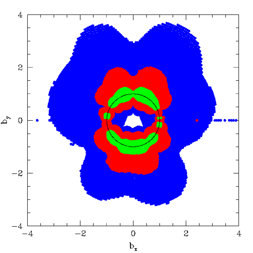
Figure 13: Planetary exclusion regions for microlensing event MOA-2003-32/OGLE-2003-BLG-219 as a function of projected coordinate $b_{x}$ and $b_{y}$ at planet-star mass ratio $q=10^{-5}$ (green), $10^{-4}$ (red) and $10^{-3}$ (blue). The source size (normalized to ${\theta}_{\rm E}$) $\rho_{*}$ is equal to 0.0007. The black circle is the Einstein ring, i.e., $b=1$.

MOA-2003-BLG-32/OGLE-2003-BLG-219, with a peak magnification $A_{\rm max}=525\pm 75$ is most sensitive to low-mass planets to date (Abe et al., 2004). However, instead of fitting the simulated binary-lens light curves to single-lens models, Abe et al. (2004) obtain their $\Delta{{\chi}^{2}}$ by directly subtracting the ${\chi^{2}}$ of a simulated binary-lens light curve from that of the light curve that is the best fit to the data. Since the source star of this event could reside in the Sagittarius dwarf galaxy, which makes the Galactic modeling rather complicated, we do not attempt to apply our entire method to this event. We calculate planet exclusion regions with the same $\Delta{{\chi}^{2}}$ thresholds (60 for $q=10^{-3}$ and 40 for the $q<10^{-3}$) as Abe et al. (2004) but using our method of obtaining $\Delta{{\chi}^{2}}$ by fitting the simulated binary-lens light curves to single-lens models. Figure 13 shows our results for the exclusion regions at planet-star mass ratios $q=10^{-5},10^{-4},$ and $10^{-3}$ for MOA-2003-BLG-32/OGLE-2003-BLG-219. The exclusion region we have obtained at $q=10^{-3}$ is about $1/4$ in vertical direction and $1/9$ in horizontal direction relative to the corresponding region in Abe et al. (2004), and the size of our exclusion region at $10^{-4}$ is about 60% in each dimension relative to that in Abe et al. (2004). Although according to our analysis, Abe et al. (2004) overestimate the sensitivity of MOA-2003-BLG-32/OGLE-2003-BLG-219 to both Jupiter-mass and Neptune-mass planets, their estimates of sensitivity to Earth-mass planets are basically consistent with our results and MOA-2003-BLG-32/OGLE-2003-BLG-219 nevertheless retains the best sensitivity to planets to date.

Figure 1: Light curve of OGLE-2004-BLG-343 near its peak on 2004 June 19 (HJD 2,453,175.7467). Only OGLE $I$-band data (open circles) are used in most of the analysis, except OGLE $V$-band data (open triangles) and $\mu$FUN $H$-band data (crosses) are used to constrain the color of the source star. All bands are linearly rescaled so that $F_{\rm s}$ and $F_{\rm b}$ are the same as the OGLE $I$-band observations. The solid line shows the best-fit PSPL model. The upper right inset shows the peak of the light curve, with the range of the simulated data points plotted by the thick line.

Figure 3: $(V_{OGLE}-I_{OGLE})/(I_{OGLE}-H_{\rm 2MASS})$ color-color diagram. All points are from matching 2MASS $H$-band data with OGLE-II $V,I$ photometry in a field centered on OGLE-2004-BLG-343. Stars on the giant branch are shown by open circles. The solid and dashed vertical lines represent the source $I_{OGLE}-H_{\rm 2MASS}$ color transformed from its $I_{OGLE}-H_{\rm\mu{FUN}}$ value and its $1\sigma$ ranges. Their intersections with the diagonal track of stars give corresponding $V_{OGLE}-I_{OGLE}$ colors, which are represented by the horizontal lines.

Figure 4: Likelihood contours ($1\sigma,2\sigma,3\sigma$) for finite-source points-lens models relative to the best-fit PSPL model. Contours with $x$-axis as $\log{u_{0}^{-1}}$ and $\log{A_{\rm max}}$ are displayed in solid and dashed lines, respectively.

Figure 7: (For real data) Planet detection efficiency of OGLE-2004-BLG-343 as a function of the planet-star separation $b$ (in the units of $r_{\rm E}$) and planet-star mass ratio $q$. The contours indicate 25%, 50%, 75%, and 90% efficiency.

Figure 9: (For fake data) Planetary detection efficiency of OGLE-2004-BLG-343 augmented by simulated data points covering the peak. as a function of the planet-star separation $b$ (in the units of ${\theta}_{\rm E}$) and planet-star mass ratio $q$. The contours represent 25%, 50%, 75%, and 90% efficiency.

Figure 10: (For real data) Planetary detection efficiency as a function of $r_{\perp}$, the physical projected star-planet distance and $m_{p}$, the planetary mass for OGLE-2004-BLG-343. The contours represent 25%, 50%, 75%, and 90% efficiency.

Figure 11: (For fake data) Planetary detection efficiency as a function of $r_{\perp}$, the physical projected star-planet distance and $m_{p}$, the planetary mass for OGLE-2004-BLG-343 augmented by simulated data points covering the peak. The contours represent 25%, 50%, 75%, and 90% efficiency.

Figure 12: Planetary detection efficiency as a function of $r_{\perp}$, the physical projected star-planet distance, and $m_{p}$, the planetary mass for OGLE-2004-BLG-343, by assuming that the blended light is due to the lens. The contours represent 25%, 50%, 75%, and 90% efficiency.

Table 1: OGLE-2004-BLG-343 Best-Fit PSPL Model Parameters

$t_{0}$(HJD’)	$u_{0}$	$t_{\rm E}$(days)	$I_{s}$	$I_{b}$	$\chi^{2}$	Degree of Freedom
$3175.7467\pm 0.0005$	$0.000333\pm 0.000121$	$42.5\pm 15.6$	$22.24\pm 0.40$	$18.08\pm 0.01$	200.1	188

References

- Abe et al. (2004) Abe, F., et al. 2004, Science, 305, 1264
- Afonso et al. (2000) Afonso, C., et al. 2000, ApJ, 532, 340
- Albrow et al. (1998) Albrow, M. D., et al. 1998, ApJ, 509, 687
- Albrow et al. (2000) Albrow, M. D., et al. 2000, ApJ, 535, 176
- Albrow et al. (2001) Albrow, M. D., et al. 2001, ApJ, 556, L113
- Alcock et al. (2001) Alcock, C., et al. 2001, Nature, 414, 617
- An & Han (2002) An, J. H. & Han, C. 2002, ApJ, 573, 351
- An (2005) An, J. H. 2005, MNRAS, 356, 1409
- Bennett & Rhie (1996) Bennett, D. P., & Rhie, S. H. 1996, ApJ, 472, 660
- Bennett & Rhie (2002) Bennett, D. P., & Rhie, S. H. 2002, ApJ, 574, 985
- Bessell & Brett (1988) Bessell, M. S., & Brett, J. M. 1988, PASP, 100, 1134
- Bond et al. (2001) Bond, I. A., et al. 2001, MNRAS, 327, 868
- Bond et al. (2002) Bond, I. A., et al. 2002, MNRAS, 333, 71
- Bond et al. (2004) Bond, I. A., et al. 2004, ApJ, 606, L155
- Carpenter (2001) Carpenter, J. 2001, AJ, 121, 2851
- Chung et al. (2005) Chung, S.-J., et al. 2005, ApJ, 630, 535
- Claret (2000) Claret, A. 2000, A&A, 363, 1081
- Cox (2000) Cox, A. N. 2000, Allen’s Astrophysical Quantities (4th Ed.; New York; Springer)
- Dominik (1999a) Dominik, M. 1999a, A&A, 341, 943
- Dominik (1999b) Dominik, M. 1999b, A&A, 349, 108
- Drake et al. (2004) Drake, A. J., Cook, K. H., & Keller, S. C. 2004, ApJ, 607, L29
- Einstein (1936) Einstein, A. 1936, Science, 84, 506
- Eisenhauer et al. (2005) Eisenhauer, F., et al. 2005, ApJ, submitted (astro-ph/0502129)
- ESA (1997) European Space Agency, 1997, The Hipparcos and Tycho Catalogues (SP-1200; Noordwijk: ESA)
- Gaudi & Sackett (2000) Gaudi, B. S., & Sackett, P. D. 2000, ApJ, 528, 56
- Gaudi et al. (2002) Gaudi, B. S., et al. 2002, ApJ, 566, 463
- Ghosh et al. (2004) Ghosh, H., et al. 2004, ApJ, 615, 450
- Gould (2000) Gould, A. 2000, ApJ, 535, 928
- Gould et al. (2004) Gould, A., Bennett, D. P., & Alves, D. R., 2004, ApJ, 614, 404
- Gould & Gaucherel (1997) Gould, A. & Gaucherel, C. 1997, ApJ, 477, 580
- Gould & Loeb (1992) Gould, A., & Loeb, A. 1992, ApJ, 396, 104
- Gould et al. (2001) Gould, A., Stutz, A., & Frogel, J. A. 2001, ApJ, 547, 590
- Griest & Safizadeh (1998) Griest, K. & Safizadeh, N. 1998, ApJ, 500, 37
- Han & Gould (1996) Han, C. & Gould, A. 1996, ApJ, 467, 540
- Han & Gould (2003) Han, C. & Gould, A. 2003, ApJ, 592, 172
- Hauschildt et al. (1999) Hauschildt, P. H., Allard, F., & Baron, E. 1999, ApJ, 512, 377
- Kervella et al. (2004) Kervella, P., et al. 2004, A&A, 426, 297
- Liebes (1964) Liebes, S., Jr. 1964, Phys.Rev., 133, 835
- Mao & Paczyński (1991) Mao, S. & Paczyński, B. 1991, ApJ, 374, L37
- Paczyński (1986) Paczyński, B. 1986, ApJ, 304, 1
- Rattenbury et al. (2002) Rattenbury, N. J., Bond, I. A., Skuljan, J., & Yock, P. C. M. 2002, MNRAS, 335, 159
- Reid (1991) Reid, N. 1991, AJ, 102, 1428
- Rhie et al. (2000) Rhie, S. H., et al. 2000, ApJ, 533, 378
- Sackett (1997) Sackett, P. D. 1997, ESO Document: SPG-VLTI-97/002 (astro-ph/9709269)
- Stanek et al. (1997) Stanek, K. Z., et al. 1997, ApJ, 477, 163
- Sumi (2004) Sumi, T. 2004, MNRAS, 349, 193
- Udalski (2003) Udalski, A. 2003, Acta Astron., 53, 291
- Udalski et al. (2005) Udalski, A., et al. 2005, ApJ, 628, L109
- Witt (1990) Witt, H. J. 1990, A&A, 236, 311
- Wolszczan & Frail (1992) Wolszczan, A., & Frail, D. A. 1992, Nature, 355, 145
- Yoo et al. (2004a) Yoo, J., et al. 2004a, ApJ, 603, 139
- Yoo et al. (2004b) Yoo, J., et al. 2004b, ApJ, 616, 1204