A combined optical/infrared spectral diagnostic analysis of the HH1 jet

Complete flux-calibrated spectra covering the spectral range from 6000Å  to 2.5$\mu$m  have been obtained along the HH1 jet and analysed in order to explore the potential of a combined optical/near-IR diagnostic applied to jets from young stellar objects. The main physical parameters (visual extinction, electron temperature and density, ionization fraction and total density) have been derived along the jet using various diagnostic line ratios. This multi-line analysis shows, in each spatially unresolved knot, the presence of zones at different excitation conditions, as expected from the cooling layers behind a shock front. In particular, a density stratification in the jet is evident from ratios of various lines of different critical density. We measure electron densities in the range 6 10²-3 10³ cm^-3 with the [S ii]  optical doublet lines, 4 10³-10⁴ cm^-3 with the near-IR [Fe ii]  lines, and 10⁵-10⁶ cm^-3 with optical [Fe ii]  and CaII lines. The electron temperature also shows variations, with values between 8000-11000 K derived from optical/near-IR [Fe ii]  lines and 11000-20000 K from a combined diagnostic employing optical [O i] and [N ii] lines. Thus [Fe ii]  lines originate in a cooling layer located at larger distances from the shock front than that generating the optical lines, where the compression is higher and the temperature is declining.

The derived parameters were used to measure the mass flux along the jet, adopting different procedures, the advantages and limitations of which are discussed. The [Fe ii] 1.64$\mu$m  line luminosity turns out to be more suitable to measure $\dot{M}_{jet}$ than the optical lines, since it samples a fraction of the total mass flowing through a knot larger than the [O i] or [S ii]  lines. $\dot{M}_{jet}$ is high in the initial part of the flow ($\sim$2.2 10^-7 M_⊙ yr^-1) but decreases by about an order of magnitude further out. Conversely, the mass flux associated with the warm molecular material is low, $\dot{M}_{H2}$$\sim$10^-9 M_⊙ yr^-1, and does not show appreciable variations along the jet. We suggest that part of the mass flux in the external regions is not revealed in optical and IR lines because it is associated with a colder atomic component, which may be traced by the far-IR [O i]63$\mu$m  line.

Finally, we find that the gas-phase abundance of refractory species, such as Fe, C, Ca, and Ni, is lower than the solar value, with the lowest values (between 10 and 30% of solar) derived in the inner and densest regions. This suggests a significant fraction of dust grains may still be present in the jet beam, imposing constraints on the efficiency of grain destruction by multiple low-velocity shock events.

1 Introduction

Highly-collimated jets of matter from young stellar objects (YSOs) are a common phenomena in star formation. These flows exhibit rich emission-line spectra over a wide range of wavelengths, from the UV to the radio. Many of the important tracers of physical conditions in the jet lie in the optical and near IR (NIR). In the optical, prominent lines such as [O i]$\lambda$6300, H$\alpha$, [N ii]$\lambda$6583, [S ii]$\lambda\lambda$6716,6731, have been widely used to derive electron density, temperature, and ionization fraction along the jet beams (e.g. Bacciotti & Eislöffel 1999, hereafter BE99, Hartigan et al. 1994). The NIR spectrum, on the other hand, comprises both important atomic lines such as [Fe ii], Pa$\beta$, [S ii], and [N i], giving complementary information on the excitation conditions (Nisini et al. 2002), as well as intense H₂ transitions from various vibrational levels, tracing the colder molecular part of the post-shocked gas (e.g. Giannini et al. 2004, Eislöffel et al. 2000). So far, the optical and NIR spectra of the same object have never been compared through combined optical/NIR diagnostics. Moreover, studies in both the optical and the infrared have mostly concentrated on limited spectral ranges, e.g. around 6500Å  and 2$\mu$m. Hence the diagnostic capabilities of lines in other parts of the spectrum have not been fully exploited. Only recently has the potential of transitions from 0.7 to 1.5$\mu$m  been highlighted by Giannini et al. (2002) and Hartigan et al. (2004).

The aim of the work described in this paper is to fill this gap and build a set of tools for a combined optical/NIR analysis of spectra of stellar jets. The advantage of such a multi-wavelength approach is twofold. On the one hand it allows us to employ ratios between lines from the same species that are well separated in wavelength thereby providing more stringent constraints on excitation conditions. This is the case, for example, for the [Fe ii]8620Å/1.64$\mu$m  and the [S ii]6716,6731Å/1.03$\mu$m  ratios, which are very sensitive to the gas electron temperature (Nisini et al. 2002, Pesenti et al. 2002). On the other hand, such an approach gives us the possibility of probing the different components of the jet cooling layers, where strong gradients are expected along the jet axis, that are not spatially resolved with current instrumentation. This, in turn, allows a better determination of parameters, such as the mass flux in the jet, which are fundamental to its dynamics and other properties. A correct derivation of this quantity is particularly important in heavily embedded sources, where the mass flux is the primary indirect manifestation of protostellar accretion activity.

In addition, a wide wavelength coverage gives us the possibiliy of observing lines of less abundant species that nevertheless contain important diagnostic information. In particular, lines from many refractory species (Ca, Ni, Cr in addition to Fe and C) can be used to derive the amount of gas depletion in the jet, thus setting constraints to the degree of dust grain destruction by shocks. The degree of grain destruction in shocks, and the relative gas-phase abundances among different species, depend on the shock properties, but also on the grain structure (Jones 2000). The latter, however, is not completely understood, although the grain composition is of crucial importance in many processes, spanning from the physics of molecular clouds to the formation of planets.

For our purpose we have observed the HH1 jet by obtaining flux calibrated spectra covering the wavelength range from 0.65 to 2.5$\mu$m, as described in Section 2. This jet, emanating from the radio source VLA1 (Strom et al. 1985) and located in the Orion L1641 molecular (D=460 pc), is well suited to test combined optical/IR analysis. It powers the prototype HH objects HH1/2 and is bright both in optical (Eislöffel et al. 1994, Hester et al. 1998, Reipurth et al. 2000) NIR H₂ and [Fe ii]  lines (Davis et al. 1994, Noriega-Crespo et al. 1994, Davis et al. 2000). A limited set of optical forbidden, as well as H₂, emission lines were analysed in the past by various authors (Solf & Böhm 1991, Noriega-Crespo et al. 1997, Eislöffel et al. 2000, Medves 2003). Here we use our new combined optical/near-IR observations to derive the relevant physical parameters ($A_{V}$, $n_{e}$, $T_{e}$, $x_{e}$, and $n_{\rm H}$) and their variation along the HH1 jet, using different line ratios capable of diagnosing regions with different excitation conditions. This is described in Section 3, while the diagnostic capabilities of specific lines are illustrated in some detail in Appendix A. In Appendix B we discuss the limitations of the widely used [Fe ii] 1.64/1.25$\mu$m  ratio to measure extinction along the line of sight.

In Section 4 we estimate the jet mass flux rate by adopting different lines and methods, discussing the limitations and advantages of the different procedures (Section 4). Finally, in Section 5, we will set constraints on the efficiency of shocks to disrupt dust grains by deriving the gas-phase abundance of different refractory species. In Section 6 we summarize our results discussing their implications for the understanding of HH jet properties.

2 Observations and results

2.1 ESO 3.6m-EFOSC2 and NTT-SofI observations

Since the aim of this project is to apply a combined optical/NIR line analysis, we obtained spectra that are as homogeneous as possible in the two wavelength ranges. Observations with the ESO 3.6-m and NTT telescopes on La Silla, Chile, were carried out during adjacent nights (7-8 January and 11-12 January 2003 for the optical and IR observations, respectively). The instruments, EFOSC2 for the optical and SofI for the infrared, had the same slit width (1$\arcsec$), corresponding to a similar spectral resolution between 500 and 600. The spatial scale of the two cameras are also comparable, being 0$\aas@@fstack{\prime\prime}$314/pixel for EFOSC2 and 0$\aas@@fstack{\prime\prime}$29/pixel for SofI. The slits were aligned along the HH1 jet at a P.A. of -36^o. The EFOSC2 observations covered the spectral range from 6015 to 10320Å  in a single grism setting, while the NTT observations were obtained with the blue (0.95-1.64$\mu$m) and red (1.53-2.52$\mu$m) grisms. Integration times were 1800s for EFOSC2 and 2400s for each of the two SofI grisms. Data reduction was performed using standard IRAF tasks. In both the optical and IR spectra we corrected for the atmospheric spectral response by dividing the object spectra by the spectrum of an O8 star showing telluric lines. The spectra were wavelength calibrated with a xenon-argon lamp, giving an uncertainty smaller than the spectral resolution element ($\sim$ 20Å). Flux calibrations were performed using photometric standards observed at an air mass difference not larger than 0.3 with respect to our target observations.

2.2 Extraction of the spectra and intercalibration

At the end of the reduction procedure, we had three individually calibrated spectral images that have to be combined to produce single spectra of the same regions. The spatial zero point was set to the position of the jet source, VLA1. To determine this in our frames, we used the bright Cohen-Schwartz (CS) star, adopting for it an angular separation of 35$\aas@@fstack{\prime\prime}$9 from VLA1 (Rodríguez et al. 2000). Figure 1 reports the emission profiles of bright lines observed in the three different images, namely [S ii] 6731Å, [Fe ii] 1.64$\mu$m  and H₂ 2.12 $\mu$m, that trace different exitation conditions and/or extinction. From the [Fe ii]  profiles, nine contiguous emission knots have been identified, named A to I following the nomenclature of Eislöffel et al. (1994) and Bally et al. (2002) . Their spatial extent is reported in Table 2. We then extracted the spectra of the individual knots and computed the line fluxes by fitting the profiles with single or, where blending is present, double Gaussian profiles. Errors to these line fluxes are measured from the rms of the adjacent continuum.

To intercalibrate fluxes for the three spectral segments of the same knot, we used the spectrum from the SofI-blue grism as a reference, normalizing the EFOSC2 spectrum to it with the [C ii]$\lambda$$\lambda$9824,9850 lines, and the SofI-red grism spectrum with the [Fe ii] 1.64$\mu$m line. We note that the intercalibration factors may differ from unity and change from knot to knot, for a variety of causes. These include different atmospheric conditions during the observations, a small misalignment of the optical and IR slits, and slighty different spatial sampling of the instruments. The net result were intercalibration factors ranging between 0.6 and 1.1 for EFOSC2 and the SofI blue grism, and between 0.9 and 1.5 for the blue and red SofI grisms. For those knots where the intercalibration lines were not observed, average factors, derived for the other knots, were used.

Figure 2 shows the complete, intercalibrated spectrum of knot G – the brightest in the optical –and in Table 1 we report fluxes and identification for all the detected lines in this knot. These, as a whole, indicate low excitation conditions, as expected for HH objects. In addition, H₂ lines from the 1-0 and 2-1 vibrational series were also observed.

Figure 1: Profiles of the [S ii], [Fe ii]  and H₂  emission along the HH1 jet. Vertical dashed lines indicate the range coadded to obtain individual knot fluxes. The [Fe ii]  profile was used to define the knot separation.

Figure 2: Combined EFOSC2 + SofI spectrum from 0.6 to 2.5$\mu$m of knot G of the HH1 jet. The stronger lines are identified.

Table 1: Lines observed in knot G of the HH1 jet

Line id.	$\lambda^{a}$	$F$	$\Delta\leavevmode\nobreak\ F$
		erg cm-2 s-1
[O i] ${}^{1}\!D_{2}-^{3}\!P_{2}$	6300	1.24 10-14	2.46 10-17
[O i] ${}^{1}\!D_{2}-^{3}\!P_{1}$	6364	4.54 10-15	2.78 10-17
H$\alpha$	6562	9.34 10-15	3.93 10-17
[N ii] ${}^{1}\!D_{2}-^{3}\!P_{2}$	6583	1.43 10-15	4.38 10-17
[S ii] ${}^{2}\!D_{5/2}-^{4}\!S_{3/2}$	6716	2.86 10-14	5.83 10-17
[S ii] ${}^{2}\!D_{3/2}-^{4}\!S_{3/2}$	6731
[Fe ii] $a^{2}\!G_{9/2}-a^{4}\!F_{9/2}$	7155	4.02 10-15	2.99 10-17
[Fe ii] $a^{2}\!G_{7/2}-a^{4}\!F_{7/2}$	7172	1.34 10-15	3.56 10-17
[Ca ii] ${}^{2}\!D_{5/2}-^{2}\!S_{1/2}$	7291	7.52 10-15	3.22 10-17
[Ca ii] ${}^{2}\!D_{3/2}-^{2}\!S_{1/2}$	7324	4.91 10-15	3.18 10-17
[Ni ii] ${}^{2}\!F_{7/2}-^{2}\!D_{5/2}$	7378	3.10 10-15	3.50 10-17
[Ni ii] ${}^{2}\!F_{5/2}-^{2}\!D_{3/2}$	7412	1.87 10-16	2.39 10-17
[Fe ii] $a^{2}\!G_{9/2}-a^{4}\!F_{7/2}$	7453	1.25 10-15	2.31 10-17
[Fe ii] $a^{4}\!P_{5/2}-a^{6}\!D_{7/2}$	7638	1.15 10-15	7.01 10-17
[Fe ii] $a^{4}\!P_{1/2}-a^{6}\!D_{3/2}$	7665	2.85 10-16	7.10 10-17
[Fe ii] $a^{4}\!P_{3/2}-a^{6}\!D_{5/2}$	7687	8.53 10-16	1.29 10-16
[Cr ii] ${}^{6}\!D_{9/2}-^{6}\!S_{5/2}$	8000	5.90 10-16	5.71 10-17
[Cr ii] ${}^{6}\!D_{7/2}-^{6}\!S_{5/2}$	8125	4.88 10-16	3.45 10-17
[Cr ii] ${}^{6}\!D_{5/2}-^{6}\!S_{5/2}$	8229	4.40 10-16	7.58 10-17
[Cr ii] ${}^{6}\!D_{3/2}-^{6}\!S_{5/2}$	8308	6.03 10-16	1.46 10-16
Ca ii ${}^{2}\!P^{o}_{3/2}-^{2}\!D_{5/2}$	8542	1.96 10-15	9.78 10-17
[Fe ii] $a^{4}\!P_{5/2}-a^{4}\!F_{9/2}$	8617	5.98 10-15	7.32 10-17
Ca ii ${}^{2}\!P^{o}_{1/2}-^{2}\!D_{3/2}$	8662	1.11 10-15	1.44 10-16
[Fe ii] $a^{4}\!P_{3/2}-a^{4}\!F_{7/2}$	8892	2.92 10-15	2.79 10-16
[Fe ii] $a^{4}\!P_{1/2}-a^{4}\!F_{5/2}$	9034	7.83 10-16	1.58 10-16
[Fe ii] $a^{4}\!P_{5/2}-a^{4}\!F_{7/2}$	9052	2.10 10-15	1.82 10-16
[Fe ii] $a^{4}\!P_{3/2}-a^{4}\!F_{5/2}$	9227	1.51 10-15	1.52 10-16
[Fe ii] $a^{4}\!P_{1/2}-a^{4}\!F_{3/2}$	9268	7.75 10-16	1.63 10-16
[C i] ${}^{1}\!D_{2}-^{3}\!P_{1}$	9824	3.60 10-15	2.19 10-16
[C i] ${}^{1}\!D_{2}-^{3}\!P_{2}$	9850	9.48 10-15	2.01 10-16
[S ii] ${}^{2}\!P_{3/2}-^{2}\!D_{3/2}$	1.029	8.77 10-16	2.10 10-16

Line id.	$\lambda^{a}$	$F$	$\Delta\leavevmode\nobreak\ F$
		erg cm-2 s-1
[S ii] ${}^{2}\!P_{3/2}-^{2}\!D_{5/2}$	1.032	1.86 10-15	2.82 10-16
[S ii] ${}^{2}\!P_{1/2}-^{2}\!D_{3/2}$	1.034
[N i] ${}^{2}\!P_{3/2,1/2}-^{2}\!D_{5/2}$	1.040	1.77 10-15	4.35 10-16
[N i] ${}^{2}\!P_{3/2,1/2}-^{2}\!D_{3/2}$	1.041
[P ii] ${}^{3}\!P_{1}-^{1}\!D_{2}$	1.148	1.02 10-15	2.01 10-16
[P ii] ${}^{3}\!P_{2}-^{1}\!D_{2}$	1.189	7.04 10-16	8.04 10-17
[Fe ii] $a^{4}\!D_{5/2}-a^{6}\!D_{9/2}$	1.192	1.21 10-15	1.06 10-16
[Fe ii] $a^{4}\!D_{3/2}-a^{6}\!D_{5/2}$	1.248	7.55 10-16	1.66 10-16
[Fe ii] $a^{4}\!D_{5/2}-a^{6}\!D_{7/2}$	1.249
[Fe ii] $a^{4}\!D_{7/2}-a^{6}\!D_{9/2}$	1.258	2.90 10-14	1.62 10-16
[Fe ii] $a^{4}\!D_{1/2}-a^{6}\!D_{1/2}$	1.271	2.06 10-15	2.32 10-16
[Fe ii] $a^{4}\!D_{3/2}-a^{6}\!D_{3/2}$	1.280	2.57 10-15	2.45 10-16
[Fe ii] $a^{4}\!D_{5/2}-a^{6}\!D_{5/2}$	1.295	4.10 10-15	2.23 10-16
[Fe ii] $a^{4}\!D_{3/2}-a^{6}\!D_{1/2}$	1.299	1.22 10-15	1.52 10-16
[Fe ii] $a^{4}\!D_{7/2}-a^{6}\!D_{7/2}$	1.321	1.03 10-14	1.77 10-16
[Fe ii] $a^{4}\!D_{5/2}-a^{6}\!D_{3/2}$	1.329	2.22 10-15	1.72 10-16
[Fe ii] $a^{4}\!D_{5/2}-a^{4}\!F_{9/2}$	1.534	4.39 10-15	1.19 10-16
[Fe ii] $a^{4}\!D_{3/2}-a^{4}\!F_{7/2}$	1.601	3.15 10-15	2.31 10-16
[Fe ii] $a^{4}\!D_{7/2}-a^{4}\!F_{9/2}$	1.645	3.27 10-14	1.92 10-16
[Fe ii] $a^{4}\!D_{1/2}-a^{4}\!F_{5/2}$	1.665	1.64 10-15	2.38 10-16
[Fe ii] $a^{4}\!D_{5/2}-a^{4}\!F_{7/2}$	1.678	3.42 10-15	2.99 10-16
H2 1–0 S(7)	1.748	1.52 10-15	3.50 10-16
H2 1–0 S(6)	1.788	1.95 10-15	3.62 10-16
H2 1–0 S(3)	1.958	1.77 10-14	2.45 10-16
H2 1–0 S(2)	2.034	1.99 10-15	1.98 10-16
H2 2–1 S(3)	2.074	8.99 10-16	9.02 10-17
H2 1–0 S(1)	2.122	5.27 10-15	1.93 10-16
H2 1–0 S(0)	2.224	1.57 10-15	1.66 10-16
H2 2–1 S(1)	2.249	8.89 10-16	1.98 10-16
H2 1–0 Q(1)	2.407	5.44 10-15	2.59 10-16
H2 1–0 Q(2)	2.414	1.60 10-15	1.84 10-16
H2 1–0 Q(3)	2.424	4.73 10-15	2.63 10-16

$a$ Air wavelengths in Å  below 1$\mu$m  and vacuum wavelengths in micron above.

2.3 Origin of the observed lines

The observed spectral range includes transitions from neutral and singly ionized atomic species which have different excitation temperatures and critical densities, thus allowing us to probe regions with different conditions. In HH jets the lines are believed to be excited in the cooling region behind a shock front. This zone, which is generally about 10¹⁴ cm wide (i.e. 0$\aas@@fstack{\prime\prime}$013 at 460pc) is not spatially resolved in our spectra, but the various lines may originate from different parts of the post-shocked regions. This is shown in Fig. 3, where we plot the emission profiles (normalized to their peak value) in the cooling region of a 70 km s^-1  shock. The profiles of $x_{e}$, $T_{e}$, and $n_{e}$ used to compute the intensity profiles were taken from the shock model of Hartigan et al. (1994) (their Fig. 1). Similar plots were shown by BE99, who noted that the optical [S ii], [N II], and [O i] transitions originate from similar regions at intermediate temperatures and ionization fractions. From our Fig. 3 we see that [S ii]  transitions at about 1.03$\mu$m come from a more compact and hot region, as they have a higher excitation temperature with respect to the optical lines. On the other hand, the emission zone of the [Fe ii]1.64$\mu$m line is broader and covers most of the post-shocked region, tracing mainly the gas at higher density and lower temperature. The profiles of other strong lines, such as [C i]9850Å  and [Ca ii]7291Å  are also indicated. In Appendix A, we describe in more detail the diagnostic capabilities of the various lines used for our analysis.

In addition to the atomic lines, we also detect H₂ emission, which is commonly observed to be spatially associated with the atomic gas in jets from young stars. The H₂ lines in the HH1 jet all come from the first two vibrational levels and thus trace temperatures of the order of 2000 K. The non-detection of lines from higher vibrational transitions, together with the relatively low reddening in at least the external sections of the jet, allows us to infer that molecular gas at higher temperatures contribute little to the overall flux (Giannini et al. 2004). The origin of the molecular emission, closely associated with gas of much higher excitation, is still not clear. The emission could originate in the post shocked layers where the gas has cooled down sufficently to become molecular again. Alternatively, it could be due to ambient material put into motion by the passage of the atomic jet or to molecular gas in the outer layers of a disk wind.

Figure 3: Relative intensity profiles of several optical and infrared lines as a function of distance from the shock-front for a 70 km s^-1 shock. These profiles have been calculated taking the temperature, density and ionization fraction profiles from Fig. 1 of Hartigan et al. (1994).

3 Derived physical parameters along the HH1 jet

Ratios of different lines can be used to constrain physical parameters, and their variation, along the jet, as described in some detail in Appendix A. However, to apply a diagnostic procedure that combines lines that are relatively far apart in wavelength, as in this case, we need to determine accurately the extinction towards each knot, and to correct the various line fluxes accordingly. To this aim, we have used the [Fe ii]  lines at 1.32 and 1.64$\mu$m, that arise from the same upper level. The reasons for our choice, instead of the more commonly used ratio [Fe ii]1.64/1.25$\mu$m, and the procedure followed, are described in Appendix B. The derived $A_{V}$ values are listed in Table 2. There is a sharp decrease in the extinction, from $A_{V}\sim$8 to 1.5 mag from the inner to the outer knots. Since for knots A to E the individual $A_{V}$ values fluctuate more than the associated errors, an average value was taken, with an uncertainty of 0.5 mag given by the dispersion of the different determinations. A visual extintion around 1.5 mag in these outer knots is in agreement with the E(B-V) value of 0.4 found by Solf et al. (1988) towards the HH1 bow shock, if a standard R=3 value is taken.

As described in Appendix A, the selected optical transitions from [S ii], [O i] and [N ii] were used to determine the electron density, electron temperature, and ionization fraction in the knots adopting the BE99 technique, which in turn allow us to derive the total density $n_{H}$=$n_{e}$/$x_{e}$ .

Given the limited spectral resolution of the EFOSC2 configuration, the [S ii] doublet at 6716, 6731Å  was not resolved sufficiently in all knots to allow us to separately measure the line fluxes. In these cases, we used data taken during a previous run with the same instrument but with higher spectral resolution, that allowed us to separate the doublet (Medves, Bacciotti & Eislöffel in prep.). We checked that the proper motion of the knots during the time interval between the two runs was negligible.

The results of our analysis of the optical lines are shown in Tab. 3 and Fig. 4, where the parameters are plotted as a function of the distance from VLA1. Moving outwards, we measure a decrease in the electron density (from $\sim$10³ cm^-3 in knots L-I to $\sim$1.5 10² cm^-3 in knots C-B), temperature (from 21000 K to 12000 K), as well as in the total density (from 1.2 10⁴ cm^-3 to $\sim$2 10³ cm^-3). Such behaviour is often observed in HH jets (BE99). The ionisation fraction $x_{e}$, on the contrary, is observed to slightly increase along the jet. This may be due to the fact that material ejected earlier had a higher degree of ionization and lower electron density. In fact, for the conditions found in stellar jets the ionization fraction is not in equilibrium with the gas thermal conditions, since the time scale for hydrogen recombination, which is proportional to 1/$n_{e}$, is generally longer than the travel time along the bright section of the jet. Therefore, the ionization fraction is essentially ‘frozen’ into the gas, and may trace past events at large distances. Alternatively, the gas may become re-ionized along the flow if, for example, the jet collides with an external clump (BE99) and an increase in ionization is induced by the UV photons created in the shock (Molinari & Noriega-Crespo 2002). This event, however, seems unlikely in our case, because the resultant shock should produce an increase in the line fluxes which is not observed.

The validity of our analysis can be checked by comparing the fluxes of other observed lines against the values predicted assuming the derived physical parameters. Fig. 5 shows such a comparison for the N and S optical and NIR lines. The ratio [S ii](1.03$\mu$m)/[S ii](6716,6731Å) indicates the presence of higher temperature components. The same information is given by [N I](1.04$\mu$m)/[N II](6583,6548Å) which, in addition, provides a check for the derived ionization fraction. In the BE99 diagnostics, in fact, the ionization fraction of hydrogen is found assuming that the O⁰ and N⁺ populations are regulated by recombination and charge-exchange with H. Thus the observed [N I]/[N II] ratio can be used to verify this assumption. We see that for both [N I]/[N II] and [S ii](IR)/[S ii](opt) the agreement between the predicted and observed values is quite good for knots H and G while the predicted value is higher than the observed one for knots L-I. Since the same effect is seen in both line ratios, the problem does not arise from an overestimate of the hydrogen ionization fraction. Also, the presence of a temperature component higher than that derived by our analysis would produce a discrepancy between the observed and predicted ratios even larger than the one we find. A better agreement between observed and predicted values in knots L-I can be obtained by assuming an $A_{V}$ value smaller than estimated, i.e. $\sim$6.5 mag instead of 8.3 mag. The agreement between observed and predicted ratio would also improve if the temperature in knots L-I is lower by about 60% with respect to the estimated value.

Figure 4: Derived physical parameters along the HH1 jet. Open circles refer to parameters estimated using diagnostics based on [Fe ii]  lines, while filled triangles refer to values determined through the BE99 technique. Error sources are described in Table 2.

Figure 5: Comparison between predicted (filled circle) and observed (crosses) dereddened ratios [NI]1.04$\mu$m/[NII]$\lambda$ 6583 (upper panel) and [SII]1.03$\mu$m/[SII]$\lambda$$\lambda$6716,6731 (lower panel). NIR lines were observed only in knots L-I, H and G.

The electron density and temperature can be measured in a completely independent way from the ratios of specific [Fe ii]  lines (see Fig. 6). Our results are also reported in Tab. 3 and plotted in Fig. 4. In Fig. 7, we see that the [Fe ii]  model fits well all the observed [Fe ii]  transitions in knot G. In fact the majority of the line ratios are reproduced within about 30-40%. Likewise, the $n_{e}$ determined from optical and NIR [Fe ii]  lines decrease with distance from VLA1, however values derived using [Fe ii]  are always a factor 3-4 higher with respect to those measured from the [S ii]  lines. Such a result has already been found in the analysis of other HH objects (Nisini et al. 2002), and indicates that the Fe emission originates from regions either denser and/or more ionized than those giving rise to the optical lines. The electron temperatures derived from the [Fe ii]  line analysis are consistent with those derived from the optical diagnostics if we consider the associated uncertainty. The average values of $T_{e}$([Fe ii]), however, are systematically lower than the $T_{e}$(opt) values. In Fig. 3 we see that such a behaviour is expected because of the different spatial distribution of Fe and optical lines in the cooling region of shocks. In fact, Fe lines originate in a wide region of the post-shocked gas having, on average, a lower temperature and higher density than the zone producing the optical lines.

Table 2: HH1 jet: physical parameters

			Diagnostics from O/S/N lines				Diagnostics from Fe lines
Knot	Da	A${}_{\rm V}\pm\Delta$A${}_{\rm V}^{b}$	n${}_{e}\pm\Delta$nec	x${}_{e}\pm\Delta$xec	n${}_{\rm H}\pm\Delta$nHc	T${}_{e}\pm\Delta$Tec	n${}_{e}\pm\Delta$nec	T${}_{e}\pm\Delta$Tec
	$\arcsec$	mag	103 cm-3		103 cm-3	K	103 cm-3	K
L-I	1.2–3.8	8.3$\pm$0.5	2.8$\pm$0.1	0.02$\pm$0.01	101.1$\pm$40.6	20 500$\pm$1900	11$\pm$1	11000${}^{+4500}_{-1500}$
H	3.8–5.5	2.9$\pm$0.5	2.6$\pm$0.1	0.06$\pm$0.01	45.4$\pm$7.9	13 000$\pm$1100	8$\pm$1	9200${}^{+2000}_{-1000}$
G	5.5–8.5	2.0$\pm$0.5	2.1$\pm$0.1	0.05$\pm$0.01	38.1$\pm$6.1	11 200$\pm$900	5$\pm$ 1	10 500${}^{+3500}_{-1500}$
F	8.5–11	2.0$\pm$0.5	1.2$\pm$0.1	0.05$\pm$0.01	26.4$\pm$6.2	11 700$\pm$1000	4$\pm$1	9800${}^{+2500}_{-1500}$
E	11–12.4	1.3$\pm$0.5	0.9$\pm$0.1	0.05$\pm$0.01	17.7$\pm$5.1	12 800$\pm$1200	30 $\pm$ 20	8200${}^{+1500}_{-1000}$
D	12.4–13.8	1.3 $\pm$0.5	0.7$\pm$0.1	0.08$\pm$0.02	8.2$\pm$3.2	13 200$\pm$1400	…	8300${}^{+1000}_{-1300}$
C	13.8–15.6	1.3$\pm$0.5	0.6$\pm$0.1	0.15$\pm$0.03	4.1$\pm$1.9	15 100$\pm$2000	…	9200${}^{+4500}_{-2500}$
B	15.6–19.1	1.3$\pm$ 0.5	0.7$\pm$0.1	0.13$\pm$0.03	5.4$\pm$2.1	14 200$\pm$1800	…	8500${}^{+3500}_{-1500}$
A	19.1-26.2	1.3$\pm$0.5	0.6$\pm$0.1	0.28$\pm$0.05	2.0$\pm$0.8	20 300$\pm$2300	…	…

^aDistance from VLA1 in arcsec
 ^bVisual extinction measured from the ratio [FeII]1.64/1.32$\mu$m (see Appendix 2 for details).
 ^cn_H is calculated as x_e/n_e. Errors are estimated using both flux uncertainties and error propagation from uncertainties in the $A_{\rm V}$ determination and in solar abundance values reported in literature (Asplund et al. 2004).

Figure 6: Diagnostic diagram based on [Fe ii]  line ratios. The grid is constructed for electron densities of 10³, 10⁴, and 10⁵ cm^-3 (dashed lines), and for electron temperatures of 4,5,6,8,10,15$\times$10³ K (solid lines). The symbols indicate the line ratios observed in the HH1 jet knots and dereddened assuming the $A_{V}$ values in Table 2.

Figure 7: Dereddened [Fe ii]  intensity ratios with respect to the 1.64$\mu$m  line in knot G (open circles) against a model with $T_{e}$=11 500 K and $n_{e}$=5 10³ cm^-3 (filled triangles). Intensities are normalized to the 1.64$\mu$m line.

3.1 Additional constraints on the excitation and physical structure

As highlighted in Appendix A, several other line ratios can further constrain jet physical parameters. Our assumption of purely collisionally excited gas can be checked using line ratios sensitive to fluorescence pumping effects. The dereddened [Ni ii]$\lambda$7412/$\lambda$7378 ratio is one of them, with expected values, for $n_{e}$ in the range 10² to 10⁵ cm^-3, between 0.04 and $\sim$0.11 for pure collisions, and $\sim$0.11 and 0.4 if fluorescence excitation is included (Bautista et al. 1996). We obtain for this ratio a value ranging from 0.04($\pm$0.02) in knot H to 0.14($\pm$0.06) in knot L-I, indicating that the excitation is mostly collisional. An additional probe of the absence of fluorescence pumping is given by the [Ca ii]$\lambda$7291/$\lambda$7324 ratio, which is expected to be 1.5 for collisional excitation (Hartigan et al. 2004). Our dereddened ratios are always consistent with this value within the errors. This implies that the permitted Ca ii transitions at 8542 and 8662Å, detected in the inner knots E to L-I, are also excited by collisions. In turn, the ratio Ca ii$\lambda$8540/[Ca ii]$\lambda$7291 can be used as diagnostic of high electron density as shown in Fig. 8. This diagram has been constructed adopting a five-levels statistical equilibrium code that uses radiative transition rates from NIST, and collisional rates from Mendoza (1983) and Chidichimo (1981). This ratio is almost independent of the temperature, while it starts to increase above $\sim$0.1 only for electron densities larger than $\sim$10⁶ cm^-3. The observed values thus imply $n_{e}$ $\sim$10⁶ cm^-3.

High electron densities along the jet are also indicated by the [Fe ii]$\lambda$7155/$\lambda$8617 ratio, which, as described in Appendix A, is a tracer of regions at densities larger than $\sim$ 10⁵ cm^-3. Figure 9 shows the observed values against the predictions of Bautista & Pradhan (1998), for $n_{e}$ in the range 10⁵–6 10⁶ cm^-3. Electron densities as high as 10⁶ cm^-3 seem to be reached in knot L-I, but a component at $n_{e}$ $\sim$10⁵ cm^-3 persists further out along the jet. Note that these values are about one order of magnitude higher than those inferred from the NIR [Fe ii]  lines. Values of electron density up to 10⁶ cm^-3 have also been inferred in the inner and denser regions of few T Tauri stars by Hartigan et al. (2004).

Figure 8: Calculated Ca ii$\lambda$8542/[Ca ii]$\lambda$7291 ratio, as a function of the electron density and temperature. The solid lines indicate the range of values observed in the HH1 jet.

Figure 9: Observed values of the ratio [Fe ii]$\lambda$ 7155/$\lambda$ 8617, which is a tracer of high density regions. The two horizontal lines indicate the value expected for densities of 10⁵ and 6 10⁶ cm^-3 in a collisionally excited gas at $T$=10000 K (Bautista & Pradhan 1998).

Finally, we point out the non-detection of the auroral optical [O ii] transitions in any of the knots. The 7331Å  line pair are never detected, while the doublet at 7321Å  could be blended with [Ca ii]7324Å . Since, however, the ratio [Ca ii]$\lambda$7291/$\lambda$7324 is always close to the value expected from theory, the contribution of [O ii]$\lambda$7321 should be negligible. This, in turn, is independent confirmation that the hydrogen ionization fraction, which is strongly tied to the O⁺/O⁰ fraction by charge exchange, is low everywhere along the jet. In knot G, for example, the upper limit [O ii]$\lambda$7331/[O i]$\lambda$6300 $\sim$8 10^-3 derived at the 3$\sigma$ level, implies an upper limit for the hydrogen ionization fraction $x_{e}$$\sim$0.1 (Hartigan et al. 2004), which is consistent with $x_{e}$=0.05 derived by us.

4 Mass flux in the jet

The knowledge of the physical conditions along the jet beam allows us to derive the mass flux carried by the HH1 jet, which is a fundamental quantity regulating the dynamics of the accretion/ejection process in protostars.

For the determination of Ṁ we exploit two different procedures. In the first method, we directly estimate the mass flux in each knot combining the total density along the jet beam with values of jet radius, $r_{J}$, and velocities, $v_{J}$ available in the literature ($\dot{M}=\mu\,m_{H}\,n_{H}\times\pi\,r_{J}^{2}\,v_{J}$, where $m_{H}$ is the proton mass, and $\mu$=1.24 is the average atomic weight). This method is not affected by uncertainties in the distance of the object and reddening estimate. On the one hand it assumes that the knot is uniformely filled at the density derived from the diagnostics, giving an upper limit to $\dot{M}$. On the other hand, such an effect is partially compensated for by the presence of regions at even higher densities in the beams than those traced by the [S ii]  lines.

The mass flux derived with this method is given in Table 3 and plotted in Fig 10. For r_J, we have taken half of the FWHM of the [S ii]  intensity profile in HST images measured by Reipurth et al. (2000), which increases from 0.1 to 1 arcsec along the jet. Jet velocities are derived from proper motion studies by Bally et al. (2002), assuming an inclination angle of 10^o (see Table 3). The derived mass flux ranges between 1 and 3 10^-7 M_⊙ yr^-1 and is fairly constant along the jet within the uncertanties.

The second method to derive the mass flux uses the observed luminosities of selected lines such as [S ii], [O I] and [Fe ii]. These lines are optically thin, thus their luminosity is proportional to the mass of the emitting gas (see e.g. Hartigan et al. 1984). We have:

$$\dot{M}=\mu\,m_{H}\times(n_{H}\,V)\times v_{t}/l_{t}$$ (1)

$$n_{H}\,V=L(line)\,\left(h\,\nu\,A_{i}\,f_{i}\,\frac{X^{i}}{X}\,\frac{[X]}{[H]}\right)^{-1}$$ (2)

where $A_{i}$, $f_{i}$ are the radiative rate and fractional population of the upper level of the considered transition, $X^{i}/X$ is the ionization fraction of the species $X$ having total abundance with respect to hydrogen $[X]/[H]$, $v_{t}$ and $l_{t}$ are the velocity and length of the knot, projected perpendicular to the line of sight.

This method is affected by uncertainties in absolute calibrations, extinction, and distance, but does implicitly take into account the volume filling factor. In practice, the latter is given by the ratio of $\dot{M}$ values derived from the two different methods. We have computed $\dot{M}$ from the luminosity of [S ii]$\lambda\lambda$ 6716,6731, [O I]$\lambda$6300, and [Fe ii]1.64$\mu$m lines, assuming all Fe is in gaseous form (Tab. 4, Fig.10). Since, as it will be discussed in section 4.4, up to $\sim$70% of Fe atoms can still be locked into grains, the derived $\dot{M}$([Fe ii]) is actually a lower limit to the real value.

Table 3: Mass flux in the jet and filling factors

knot	$v_{\rm tan}$a	$r_{jet}$b	$\dot{M}$($n_{\rm H},r_{j},v_{j}$)c	$\dot{M}$([S ii])d	$ff$([S ii])e	$\dot{M}$([Fe ii])d	$\dot{M}$(H2)f
	km s-1	arcsec	M⊙ yr-1	M⊙ yr-1		M⊙ yr-1	M⊙ yr-1
L-I	300	0.1	1.8 10-7	2.4 10-7	1.3	2.2 10-7	4.7 10-9
H	300	0.15	1.6 10-7	3.6 10-8	0.2	7.1 10-8	4.7 10-10
G	305	0.2	2.4 10-7	6.9 10-8	0.3	1.0 10-7	1.9 10-9
F	300	0.3	3.1 10-7	3.7 10-8	0.1	5.2 10-8	8.9 10-10
E	281	0.3	2.3 10-7	1.8 10-8	0.08	4.4 10-8	1.3 10-9
D	300	0.35	1.5 10-7	1.5 10-8	0.1	3.8 10-8	1.8 10-9
C	296	0.4	9.7 10-8	1.1 10-8	0.1	2.9 10-8	1.6 10-9
B	317	0.5	1.7 10-7	7.5 10-9	0.04	2.4 10-8	2.1 10-10
A	311	0.5	7.6 10-8	5.1 10-9	0.07	2.8 10-9	1.1 10-9

^a taken from the proper motion study by Bally et al. (2002). Total velocities ($v_{jet}$) have been derived from these values assuming an inclination angle of 10⁰.
 ^b taken from the FWHM intensity transverse profiles in HST images of Reipurth et al. (2000)
 ^c $\dot{M}$($n_{\rm H},r_{j},v_{j}$) = $\mu\,m_{H}\,n_{H}\times\pi\,r_{jet}^{2}\,v_{jet}$, where $n_{H}$ is the total density reported in Table 2. Volume filling factors equal to unity are assumed.
 ^d $\dot{M}$ measured from the luminosities of the [S ii]$\lambda$$\lambda$ 6716,6731 lines and [Fe ii]1.64$\mu$m line.
 ^e Volume filling factor estimated from the ratio between the observed and predicted line luminosities (see text). They are also equal to the ratio between $\dot{M}$ and $\dot{M}$($n_{\rm H},r_{j},v_{j}$) derived from line luminosities.
 ^f $\dot{M}$ measured from the luminosity of the H₂ 2.12$\mu$m line, assuming the H₂ temperature estimated from the ratio of the different H₂ observed lines.

Figure 10: Comparison of the Ṁ determinations along the HH1 jet derived adopting different methods and lines. Filled squares refer to Ṁ values directly measured from our derived total density and the knot radius taken from Reipurth et al. (2000), assuming complete beam filling. Filled circles are mass loss rates estimated from [S ii]$\lambda\lambda$6716,6731 and [OI]$\lambda$6300 luminosities. The two values coincide inside the symbol. Finally, crosses and triangles refer to the Ṁ value derived from the [Fe ii]1.64$\mu$m and H₂ 2.12$\mu$m luminosities.

Fig. 10 illustrates the Ṁ values obtained with the different methods. We note that the values derived from line luminosities are lower than those calculated from the jet density and radius, and fall off along the jet, indicating a decrease of filling factor. In fact, measuring the volume filling factor ($ff$) by comparing the observed luminosity with that expected from the considered volume, one finds that $ff$ varies from $\sim$1 to $\sim$0.06 from knot L-I to knots A-B (Table 3). This behaviour is not unexpected, as the furthest knots have a larger volume filled with more diffuse gas, while the knots closer to the star are more dense and compact.

In Fig. 10 we note that the mass flux derived from [Fe ii]  line luminosity is larger than $\dot{M}$([S ii],[O i]), at least from knot H outwards. This suggests that the higher $n_{e}$ values, given by the [Fe ii]  diagnostic, come from gas with higher average density than in the [S ii]  line emitting region, rather than from gas with a higher ionization fraction. Thus the [Fe ii]  luminosity is probably a better tracer of the mass flux than the [O i] or [S ii]  line luminosity, since the former traces a larger portion of the total mass flowing through a single knot.

Ṁ derived from line luminosities, which takes into account the filling factor, decreases with distance from the source. A constant mass flux along the jet is expected if the flow is stationary, since the decrease in the total density should be compensated for by the larger jet radius. A mass flux decrease can be due to a change in the jet physical conditions: if the gas recombines and the temperature decreases, the bulk of the flowing mass may be mainly in neutral atomic or molecular form and thus not be traceable through its ionic emission. To gauge the mass flux associated with the molecular components we have determined $\dot{M}$(H₂) using the 2.12$\mu$m  line luminosity. The temperature of the warm H₂  gas is 2000–2500 K, as derived from the ratios of the dereddened line fluxes. Then, the total N_H2 column density is measured by comparing the intrinsic (per unit mass) and observed flux of the 1-0 S(1) 2.12$\mu$m line. The H₂  tangential velocity has been assumed equal to that derived from optical lines, following Noriega-Crespo et al. (1997), who measured H₂  knot proper motions comparable to those obtained from atomic emission lines.

Our values of $\dot{M}$(H₂ ) range between 2 10^-10 and 2 10^-9 M${}_{\odot}\,yr^{-1}$, and are therefore about 2-3 orders of magnitude lower than those derived from the atomic lines. Moreover, Ṁ(H₂) does not increase with distance. Thus it is unlikely that the decrease of the mass flux derived for the atomic/ionic component is due to atomic gas turned into molecular material. Other contributions, however, such as atomic gas at low temperature, not emitting in the optical and near IR, may become important to the bulk of mass flow. In this regard, we note that strong [OI]63$\mu$m line emission, which traces shocked atomic gas at temperatures below 5000 K, has been detected by ISO in a 70$\arcsec$ beam centred on VLA1 (Giannini et al. 2001, Molinari & Noriega-Crespo 2001). Similar 63$\mu$m emission has also been found towards HH1 and HH2, suggesting that such emission is not excited in the source circumstellar envelope, but derives from both the shocked gas and the diffuse PDR of the hosting cloud. This latter contribution has been estimated to account for about 50% of the total [OI] luminosity. Excluding the PDR contribution and estimating the mass flux from the [OI]63$\mu$m  luminosity (Hollenbach 1985), we derive $\dot{M}$([OI]63$\mu$m) $\sim$ 3 10^-6 M${}_{\odot}\,yr^{-1}$. Such a large value suggests that a significant part of the mass flux may be due to a warm atomic component. FIR observations at resolution higher than that available with ISO, may be obtained in the near future with SOFIA and Herschel, and will allow us to gain a more complete picture.

Finally, we note that $\dot{M}$(H₂) in the HH1 jet is on average lower by one or two orders of magnitude with respect to the values derived by Davis et al. (2001, 2003) for other small-scale H₂  jets from embedded sources. These authors also find that $\dot{M}$(H₂) and Ṁ(FeII) are roughly comparable for the majority of the objects in their sample. In contrast, our estimates for HH1 show its this jet, despite its origin from an embedded source, presents characteristics similar to jets from more evolved YSOs. In such sources the molecular component contributes little to the jet excitation and dynamics in comparison to the atomic component.

We also note that the molecular outflow associated with the VLA1 source is weak and less energetic than other outflows from Class 0 sources (Moro-Martín et al. 1999). The momentum flux deduced by our observations of the atomic jet ($\sim$3 10^-5 M${}_{\odot}\,km\,s^{-1}\,yr^{-1}$) is comparable to that estimated for the associated CO outflow (Correia et al. 1997). All thi evidence suggests that around VLA1 the density of molecular material is low and thus that the dynamics of the flow is mainly determined by the atomic gas.

5 Abundances of refractory elements

The observed wavelength range includes several lines from refractory species. In addition to Fe, we detected transitions from C, Ca, Ni and Cr. These species are expected to be largely depleted in neutral or molecular interstellar regions, while their gas phase abundance is enhanced in shocked regions where the dust grains have been at least partially destroyed either by sputtering or by photoevaporation (e.g. Draine 2003). Therefore, the determination of gas phase abundances can provide constraints on dust properties and structure, on dust destruction mechanisms and on how such mechanisms depend on physical parameters such as jet velocity and excitation conditions. In this regard we note that the different species are expected to follow selective patterns for their erosion from the dust grains, and thus the fraction of their gas-phase abundance can be different and give further indications of dust grain reprocessing.

To derive quantitatively the gas-phase elemental abundance, however, one has to rely on comparing emission of refractory and non-refractory species that originate in the same region. In this way, the difference between predicted ratios of lines, calculated with the determined values of $T_{e}$, $n_{e}$ and $x_{e}$, and the observed ratios gives indications on the depletion of the refractory species with respect to the assumed solar abundance. For Fe this procedure is quite complicated, and contrasting results have been reported for HH objects (see e.g. Böhm & Matt 2001, Beck-Winchatz et al. 1996, Nisini et al. 2002). The fact that the Fe spectrum is consistent with physical conditions different from those inferred from the optical lines (e.g. [S ii]$\lambda$6716 and [O i]$\lambda$6300) gives strong limitations to a diagnostics based on a comparison between such lines.

This is demonstrated in Figure 11, which is a plot of the line ratios [Fe ii]$\lambda$8617/[S ii]$\lambda\lambda$6716,6731 and [Fe ii]$\lambda$8617/[O i]$\lambda$6300, assuming a Fe gas-phase abundance equal to solar (3 10^-5, Grevesse & Sauval 1998). The [Fe ii]$\lambda$8617 line has been chosen because its spatial distribution is similar to the distribution of the [S ii]  and [O i] lines, as shown in Figure 3. However, Figure 11 shows that the predicted ratios, assuming for all lines the physical conditions derived from the BE99 analysis, underestimate the observed values and, in fact, would suggest Fe gas phase abundances larger than solar.

We have then considered the ratio [Fe ii]1.25$\mu$m/[P ii]1.18$\mu$m (Figure 12). Phosphorus is a non-refractory species and its 1.18$\mu$m line has about the same excitation conditions as the [Fe ii]1.25$\mu$m line. As shown in Oliva et al. (2001), the ratio [Fe ii]1.25/[P ii]1.18 should be about [Fe/P]/2. Assuming solar abundances ([Fe/P]$\sim$ 112) we find [Fe]_gas/[Fe]_solar $\sim$0.7 for knots G and F and $\sim$0.2-0.3 for the internal knots L-I and H, in line with values derived in Nisini et al. (2002) for other HH objects. Finally, a Fe gas-phase abundance lower than solar is also inferred from a comparison of [Fe ii]  lines and Pa$\beta$ as in Nisini et al. (2002). In knot G, taking a Pa$\beta$ upper limit of 5 10^-16 erg s^-1 cm^-2, $T_{e}$=11 000 K and $x_{e}$=0.05, we derive a lower limit of [Fe]_gas=0.1 [Fe]_solar from the plot in Fig. 13 of Nisini et al. (2002).

The gas phase abundance of C and Ca is more easily derived from a comparison with the [S ii]  optical lines assuming the same excitation conditions (see Fig. 3). Figure 13 shows the comparison between the observed and predicted ratios [C i]$\lambda\lambda$9824,9850/[S ii]$\lambda\lambda$6716,6731 and [Ca ii]$\lambda\lambda$7291,7324/[S ii]$\lambda\lambda$6716,6731.

While Ca can be assumed to be completely ionized, the fraction C⁰/C_tot has been computed with an ionization balance between collisional and charge-exchange ionization, and direct/dielectronic recombination (rates from Stancil et al. (1998) and Landini & Monsignori Fossi (1990)). Figure 13 shows that the observed [C i]/[S ii]  ratio decreases towards the source, in contrast to what can be expected theoretically. In knots L-I, however, the higher temperature causes C to become almost completely collisionally ionized and the theoretical ratio is also reduced. The discrepancy between observed and expected [C i]/[S ii]  ratios can be interpreted as due to a decrease in the C gas-phase abundance. This behaviour can be correlated to the increase of the total density from about 5 10³ to 1.2 10⁵ cm^-3 going from knots A-C to knots L-I, since the efficiency of depletion increases with the density. On the other hand, the higher temperature of knot L-I may cause dust evaporation of C to compete against depletion.

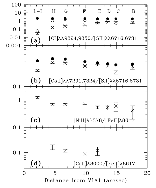
In Fig. 13 we also show that the observed [Ca ii]/[S ii]  ratio is smaller than predicted for knots F to L-I, although Ca depletion is lower than for C. To check if selective depletion is present among other species, we have plotted in Figure 13 the [Ni ii]$\lambda$7378/[Fe ii]$\lambda$8617 and [Cr ii]$\lambda$8000/[Fe ii]$\lambda$8617 ratios observed in the various knots. There is evidence that the [Ni ii]$\lambda$7378/[Fe ii]$\lambda$8617 ratio decreases with distance. Since Ni⁺ and Fe⁺ coexist, and the two lines have the same excitation conditions (Bautista et al. 1996), we interpret the observed decrease as a change in the [Ni]/[Fe] gas abundance ratio. In this respect it is interesting to note that Beck-Winchatz et al. (1996) found a Fe abundance close to solar in the HH1 bow shock, but here the Ni/S ratio was 10 times the solar value.

The presented analysis, therefore, shows that a certain degree of depletion of the refractory elements is present, an effect which is apparently selective, being higher for Fe and C. This shows that dust grains are not completely destroyed in stellar jets, and that the number of refractory atoms released in the gas phase is an inverse function of the total density. In fact, models for dust reprocessing in shocks show that shattering processes, and grain-grain collisions, are able to destroy only a few percent of large grains for shock velocities $v_{s}\ga$ 10 km s^-1  (Draine 2003). At the same time, sputtering in fast shocks produces complete dust destruction for $v_{s}>$ 100km s^-1  (Jones 2000). Since shocks in stellar jets, like the HH1 jet, have velocities no larger than 40-50km s^-1, we would expect that a large fraction of dust grains survive shocks and contribute to the observed partial depletion of refractory elements. Moreover, our results also show that multiple low velocity shock events, such as those occurring in protostellar jets, are not 100% efficient in completing the dust destruction process.

Figure 11: Ratios of [Fe ii]8617Å  line with respect to [S ii]$\lambda$$\lambda$ 6716,6731 and [O i]$\lambda$6300 in the various knots. Crosses: measured de-reddened values. Filled circles: predicted values assuming $T_{e}$ and $n_{e}$ derived from the BE99 analysis. Fe and S have been assumed completely ionized once, while the O⁺/O⁰ fraction has been calculated using the ionization model for this species.

Figure 12: Observed [Fe ii]1.25$\mu$m/[PII]1.18$\mu$m ratios in knots L-I, H, G and F. The line represents the predicted value expected if all the iron is in gaseous form and assuming a [Fe]/[P] solar abundance ratio of 112.

Figure 13: Dereddened ratios of lines from refractory species (crosses): (a) [C i]$\lambda$$\lambda$ 9824,9850/[S ii]$\lambda$$\lambda$ 6716,6730, (b) [Ca ii]$\lambda$$\lambda$ 7291,7324/[S ii]$\lambda$$\lambda$ 6716,6730, (c) [Ni ii]$\lambda$7378/[Fe ii]$\lambda$8617, (d) [Cr ii]$\lambda$8000/[Fe ii]$\lambda$8617. In panels (a) and (b), filled circles are the predicted values assuming Ca, C and S have solar abundances, C all neutral and Ca, S all singly ionized. Open circles in panel (a) refer to predictions where the C⁰/C⁺ abundance ratio has been computed through ionization equilibrium analysis.

6 Summary

We have presented a new combined optical/NIR analysis of flux calibrated spectra of the HH1 jet. The simultaneous use of several diagnostic lines has proven to be very powerful in probing the density and temperature stratification inside the jet knots, and has allowed us to obtain a very detailed picture of the jet physical structure and excitation even from moderate spectral and spatial resolution observations.

Using different line ratios, we have derived visual extinction, electron density, temperature and ionization fraction as a function of distance from the driving source. The electron density from the [S ii]  doublet decreases from 3 10³ cm^-3 in the L-I knots (at d$<$4^′′ from VLA1) to $\sim$600 cm^-3 in the A-D knots far from the star. Conversely, $n_{e}$ values between 10⁴ and 4 10³ cm^-3 are derived in the same knots from [Fe ii]  line IR ratios. Finally, the use of very high density probes, such as [Fe ii] $\lambda$7155/8617 and Ca ii$\lambda$8542/[Ca ii]$\lambda$7291, supports the presence of jet components at even higher electron densities, ranging from 10⁵ to 10⁶ cm^-3. Such a stratification presumably originates in the different layers of a post-shocked gas. This is reasonable since the post-shock cooling distance is expected to range between $\sim$10¹⁴ and 10¹⁶ cm (Hartigan et al. 1987, see also Fig. 1), i.e. smaller than our spatial resolution. Our conclusion is also supported by the temperature values inferred from the [Fe ii]  optical/NIR ratios, which are lower in comparison to those derived from using optical line diagnostics. Fe emission therefore traces post-shocked regions located at larger distances from the shock front than [S ii]  lines, where the compression is higher and the temperature is declining.

The ionization fraction, derived using the BE99 diagnostics, is rather low ($x_{e}\sim$0.02-0.1) which is also supported by the non-detection of the [OII] auroral lines at 7321 and 7331Å. Several line ratios have been also used to exclude the presence of fluorescence excitation even in the knots closest to the source. This implicitly validates the diagnostic procedures we use, which assumes that the gas radiative properties are regulated by collisional excitation.

If we assume that the ionization fraction is almost constant throughout most of the post-shocked line emitting region, as the profile in Fig. 1 would suggest, we deduce, in the innermost jet region, a total density as high as 5 10⁷ cm^-3. Moreover, the range of total densities probed by our analysis implies that in each knot a compression factor C = $n_{\rm postshock}/n_{\rm preshock}$ of at least 10² is reached. For comparison, values of C lower than $\sim$100 are derived from dissociative shocks with velocity ranging from 30 to 100 km s^-1  (Hartigan et al. 1994).

The mass flux in the jet has been determined for each knot using two methods. In the first $\dot{M}$ is calculated combining the estimated $n_{H}$ values with the jet radius and velocity taken from the literature ($\dot{M}$($n_{H},r_{j},v_{j}$)). In the second we used a comparison of observed and predicted total luminosity of the [S ii], [O i], and [Fe ii]  lines. In the jet section closest to the source (i.e. knots L-I) both methods suggest a value of $\sim$2 10^-7 M_⊙ yr^-1. Conversely, as we move away from the driving source we find discrepancies between the results from the two methods. The $\dot{M}$($n_{H},r_{j},v_{j}$) value represents an upper limit to the mass flux, since one makes the assumption that the jet is completely filled by gas at the estimated density. Conversely, $\dot{M}$([SII],[OI]) calculated from line luminosities, takes into account the proper filling factor, but underestimates the real $\dot{M}$ value, since in this case one does not include the higher density gas regions. $\dot{M}$([FeII]) is intermediate between these two values, and is probably a better tracer of the global mass flux through the jet.

$\dot{M}$([FeII] is found to decrease with the distance from the driving source, from 2 10^-7 in knots L-I down to $\sim$3-5 10^-9 M_⊙ yr^-1 in knot A. Such a decrease may indicate that in the more distant regions of the jet an atomic component at $T<5000$ K (as traced by the [OI]63$\mu$m emission observed by ISO) becomes important and contributes to the bulk of the mass flow. The mass flux due to the warm molecular H₂ gas has also been estimated and it turns out to be always smaller than the other values by one or two orders of magnitude.

Finally, the presented observations suggest that the refractory elements are still partially depleted with respect to the assumed solar abundance by fractions which varies from less than 10% in the low density regions up to $\sim$90% for C, $\sim$70% for Fe and $\sim$50% for Ca in the inner and densest knots. This is a result expected in relatively low-velocity shocks, since the complete destruction of dust by shattering processes is predicted only for shock velocities larger than 50-100 km s^-1. It also indicates that the action of several low-velocity shock events during the jet lifetime is not effective in producing a complete destruction of dust grains. While we found that there is evidence of depletion depending on gas density, an analysis performed on a larger number of jets is needed to properly determine the dependence of the gas-phase abundances of refractory elements on jet excitation conditions. In addition, the observation of a selective pattern for the depletion of different elements needs to be investigated further since it may provide important information on dust grain composition and properties.

Appendix A Diagnostic capabilities of the observed lines

A.1 Oxygen, Nitrogen and Sulphur lines

The forbidden lines from O, N, S in the optical range are powerful diagnostic tools for stellar jets, as discussed in BE99, Dougados et al. (2000), Hartigan et al. (2004). In particular, the ratio of [S ii]$\lambda$6716 and $\lambda$6731 is sensitive to electron densities in the range 50-2 10⁴ cm^-3, this latter value being the critical density for collisional excitation. Furthermore, BE99 have developed a method to derive the hydrogen ionization fraction $x_{e}$ and the electron temperature T_e from the observed ratios [O i]$\lambda$$\lambda$6300,6363/[N ii]$\lambda$$\lambda$6583,6548 and [O i]$\lambda$$\lambda$6300,6363/[S ii]$\lambda$$\lambda$6716,6731. The technique is based on the fact that in typical conditions for the beams of stellar jets the hydrogen ionization fraction is primarily determined by charge-exchange with oxygen and nitrogen atoms, while collisional ionization of H and photoionization do not make a large contribution until the shock velocity exceeds 100 km s^-1. Such a velocity, however, is only reached in the large bow-shocks at the head of the jets, while those in the beam are generally not larger than 30-40 km s^-1. An additional assumption is that S is all singly ionized. Such an assumption is motivated by the large I.P. of S⁺ (50 eV) and by the non-detection of the [S iii] and [S i] lines at 9533Å  and 1.082$\mu$m respectively, in any of our spectra. More details can be found in BE99 and Bacciotti (2002). The jets analysed with this technique in previous studies typically have 0.01$<x_{e}<$0.6 and 7000$<T_{e}<$2 10⁴. When using the BE technique a set of elemental abundances has to be assumed. In this study we have adopted solar abundances from Grevesse & Sauval (1988).

[S ii]  and [N i] lines are also observed in the NIR part of the spectrum. They consist of four closely spaced lines for each species ([S ii]  at 1.029, 1.032, 1.034, and 1.037$\mu$m  and [N i] at 1.0400, 1.0401, 1.04100, and 1.04104$\mu$m ) having excitation energies higher than the optical lines ($\sim$35 000 and 40 000 K, respectively). Thus, in principle, the [S ii]1.03$\mu$m lines can be combined with the optical [S ii]  lines to give an independent estimate of $T_{e}$. On the other hand, the [N i] lines at 1.04$\mu$m  can be used with the [N ii] optical lines to determine the ionization fraction.

A.2 Iron lines

Most of the observed [Fe ii]  lines originate from transitions among the first 16 fine structure levels. As illustrated in Nisini et al. (2002), electron densities in the range 10³–10⁵ cm^-3 can be derived from line ratios of IR lines, 1.64/1.60$\mu$m and 1.64/1.53$\mu$m in particular, while the ratios 1.64/1.25$\mu$m and 1.64/1.32$\mu$m can be used to determine the visual extinction (see Appendix B). In the optical part of the spectrum, we also observe transitions coming from levels at higher excitation temperatures. Consequently, the ratios between selected optical and IR [Fe ii]  lines are a good diagnostic tool for the measurement of the electronic temperature in the range 5 000–20 000 K (Nisini et al. 2002, Pesenti et al. 2003).

The combination of the IR and optical spectrum of ionized Fe can therefore be used effectively to give an independent diagnostic of temperature and density, which, relying on ratios from lines of a single species, is not affected by any assumption of abundances. For our analysis, we use a statistical equilibrium model which considers the first 16 [Fe ii]  levels, the collisional strengths from Zhang & Pradhan (1995) and the transition probabilities from Nussbaumer & Storey (1988). An example of a diagnostic diagram for such an analysis is shown in Fig. 6. Similar diagrams are also presented in Nisini et al. (2002) and Pesenti et al. (2003).

We have also detected, in some of the knots, the lines at 7155, 7172, and 7453Å  which connect the doublet $a^{2}\!G_{9/2,7/2}$ with the $a^{4}\!F$ levels. As shown in Bautista & Pradhan (1998) and Hartigan et al. (2004), the ratio between the 7155Å  and 8617Å  transitions is sensitive to electron densities in the range $n_{e}\sim$10⁵-10⁷ cm^-3, signalling the presence of high density conditions.

A.3 Other atomic/ionic lines

Other prominent atomic/ionic lines observed in the spectra include transitions from the refractory species [C I], [Ca II], [Cr II] and [Ni II].

The [C I]$\lambda\lambda$9824,9850 lines can be excited both by collisions with neutrals and electrons in a partially ionized medium, or by recombination (Escalante & Victor 1990). In this latter case, other lines from the recombination cascade, such as the 1.07 and the 1.17$\mu$m transitions, which are expected to be only a factor 1-10 weaker than the 9840Å  lines, should also be detected (Walmsley et al. 2000). Their non-detection in any of our spectra would imply that the [C I] lines are collisionally excited in the HH1 jet. The presence of strong [C I] lines also implies low excitation conditions, and in fact the ratio [C I]/H$\alpha$ is a very good indicator of excitation in HH objects.

We detect [Ca II] lines originating from transitions among the first five Ca⁺ levels. In particular, we detect the two forbidden lines at 7291 and 7324Å  connecting the ${}^{2}\!D_{5/2,3/2}$ levels with the ground state, as well as the permitted lines at 8542 and 8662Å, connecting the ${}^{2}\!P_{3/2,1/2}$ levels with the ${}^{2}\!D_{5/2,3/2}$. These latter two transitions can be collisionally excited, being only at 25 000 cm^-1 from the ground state or, alternatively, photoexcited through the Ca II K and H lines. Thus, the ratios among the observed lines can be used as a diagnostic to see if fluorescent excitation is important.

Ni⁺ is expected to coexist with Fe⁺, given their similar ionization potential (7.9 and 7.6 eV, respectively). It has been found to be overabundant with respect to the solar value both in HH objects and in other gaseous nebulae such as supernova remnants (Beck-Winchatz et al. 1996, Bautista et al. 1996). In the latter, the observed strong [Ni ii] emission has been explained by the contribution of fluorescent excitation in a low density environment. Indeed, the ratio between the optical lines, at 7412 and 7378Å  can be used as a discriminator between collisional and fluorescent excitation (Bautista et al. 1996).

Finally, in the spectra of the brightest knots we also detected the two [P ii] transitions at 1.148 and 1.189$\mu$m. Such lines have excitation properties very similar to the [Fe ii]  lines but P is a non-refractory element. This makes the IR ratio [Fe ii]/[P ii] a good tool to estimate Fe depletion (Oliva et al. 2001).

Appendix B Determination of $A_{V}$ from [Fe ii]  lines

Visual extinction can be estimated from pairs of lines originating from the same upper level, providing the emission is optically thin. In this case, their theoretical intensity ratio depends only on frequency and transition probabilities, and not on physical conditions in their emission region. There are several [Fe ii]  lines which have this property, and the ratio [Fe ii]1.64/1.25$\mu$m (hereafter 1.64/1.25) is most commonly used for this purpose, as these lines are the brightest of the near IR [Fe ii]  spectrum (Gredel et al. 1994, Nisini et al. 2002). Among detected [Fe ii]  lines, the bright transition at 1.32$\mu$m also comes from the same upper level as the 1.64 and 1.25$\mu$m lines, and thus the ratio [Fe ii]1.64/1.32$\mu$m (hereafter 1.64/1.32) gives an independent check of reddening. In Fig. 14 we plot the observed 1.64/1.25 and 1.64/1.32 ratios in the different jet positions. This plot shows the reddening variations along the jet irrespective of the absolute value of the visual extinction, indicating that the reddening is almost constant from knots A to H and sharply increases in knots L-I. This is consistent with Reipurth et al. (2000) who estimated that the visual extinction in the inner portion of the jet is larger, by $\sim$ 4 mag, than that in the external knots. To convert the observed ratios to A_V values, we adopt the radiative transition probabilities given by Nussbaumer & Storey (1988), which imply intrinsic ratios 1.64/1.25=0.73 and 1.64/1.32=2.81. We further use an interpolation of the near IR Rieke & Lebofsky (1985) extinction law of the form $A_{\lambda}/A_{V}=0.42\,\lambda(\mu m)^{-1.75}$ (Draine 1988). In Figure 14 we also plot the $A_{V}$ values derived from the two line ratios. Note that the extinction estimated from the 1.64/1.25 ratio is always about a factor of two larger than the values estimated from the 1.64/1.32 ratio.

Figure 14: Observed variations along the HH1 jet of the reddening sensitive [Fe ii]  line ratios 1.64/1.25$\mu$m (a) and 1.64/1.32$\mu$m (b). Panel (c) shows the derived $A_{V}$ values from the two ratios assuming an interpolation of the Rieke & Lebofsky (1985) extinction law and transition probabilities from Nussbaumer & Storey (1988). Circles and triangles are the $A_{V}$ values measured from the 1.64/1.25 and 1.64/1.32 line ratios, respectively.

Such differences can be critical when estimating the intrinsic ratio of lines far apart in wavelength. Thus, we need to investigate the possible causes of such a discrepancy in more detail.

The observed discrepancy cannot originate from any systematic observational effect. The three lines (1.64, 1.25, and 1.32$\mu$m) are all observed with the same grism and thus are not affected by any problem of intercalibration. They are detected at large S/N, implying that any contamination due to OH sky line residuals (which could affect the 1.64$\mu$m line) is negligible. We then checked for observations of these three lines in other objects. In Nisini et al. (2002) the $A_{V}$ values estimated from the 1.64/1.25 ratio in a number of HH objects were always higher than the value derived from optical observations. Moreover we have verified that extinction values derived from the 1.64/1.32 ratio are more consistent with the optical determinations. The same effect, i.e. $A_{V}(1.64/1.25)>A_{V}(1.64/1.32)$, can be found in various gaseous nebulae where these lines have been detected with sufficent accuracy (e.g. Orion B, Walmsley et al. 2000, and supernova remnants, Oliva et al. 1990). Finally, in the HH1 bow shock Noriega-Crespo & Garnavich (1994) estimated an Av = 6.7 using the 1.64/1.25 ratio, pointing out the discrepancy between this value and that measured through optical line ratios.

The most likely explanation for such a discrepancy is probably uncertainty in the transition probabilities of the lines involved. More recent calculations of such probabilities, by Quinet et al. (1997), show discrepancies with respect to the Nussbaumer & Storey (1988) values as large as 20%. With the Quinet et al.(197) $A$ values, the theoretically expected ratios become 1.64/1.25=0.965 and 1.64/1.32=3.67 . If applied to our data, such ratios produce on average $A_{V}$ smaller than the values derived with the NS88 data, but the discrepancy between the 1.64/1.25 and 1.64/1.32 estimated values remains. In knot G, for example, we derive, with the Quinet et al. (1997) values, $A_{V}(1.64/1.25)$= 1.6 mag, but $A_{V}(1.64/1.32)<0$. In general, the $A_{V}(1.64/1.32)$ value estimated with the parameters by Quinet et al. (1997) tends to be always negative, suggesting that the theoretical value is probably overestimated.

Finally, we point out that the higher $A_{V}$ values derived from the 1.64/1.25(NS88) ratio, turn out to be inconsistent with the ratios of other observed transitions irrespective of the assumed physical conditions. For example the [Fe ii]1.64/0.862 ratio in knot G, if corrected for an $A_{V}$ larger than 4, is outside the range of expected theoretical ratios for any temperature (see Fig. 4). The same applies to the ratio [S ii]0.67/1.03 (see also the discussion in Section 4.2). In view of the above discussion, we suggest that the 1.64/1.32 ratio from NS88 gives, for the moment, the most reliable determination of the $A_{V}$ value.