Crossing of the $w=-1$ Barrier by D3-brane
Dark Energy Model

Abstract

We explore a possibility for the Universe to cross the $w=-1$ cosmological constant barrier for the dark energy state parameter. We consider the Universe as a slowly decaying D3-brane. The D3-brane dynamics is approximately described by a nonlocal string tachyon interaction and a back reaction of gravity is incorporated in the closed string tachyon dynamics. In a local effective approximation this model contains one phantom component and one usual field with a simple polynomial interaction. To understand cosmological properties of this system we study toy models with the same scalar fields but with modified interactions. These modifications admit polynomial superpotentials. We find restrictions on these interactions under which it is possible to reach $w=-1$ from below at large time. Explicit solutions with the dark energy state parameter crossing/non-crossing the barrier $w=-1$ at large time are presented.

1 Introduction

The combined analysis of the type Ia supernovae, galaxy clusters measurements and WMAP data provides an evidence for the accelerated cosmic expansion [1, 2, 3]. The cosmological acceleration strongly indicates that the present day Universe is dominated by smoothly distributed slowly varying Dark Energy (DE) component. The modern constraints on the DE state parameter are around the cosmological constant value, $w=-1\pm 0.1$[3, 4] and a possibility that $w$ is varied in time is not excluded. From the theoretical point of view there are three essentially different cases: $w>-1$ (quintessence), $w=-1$ (cosmological constant) and $w<-1$ (phantom) ([5, 6, 7] and refs. therein).

Since from the observational point of view there is no barrier between these three possibilities it is worth to consider models where these three cases are realized. Under general assumptions it is proved in [8] that within one scalar field model one can realize only one possibility: $w\geq-1$ (usual model), or $w\leq-1$ (phantom model). It is interesting that the interaction with the cold dark matter does not change the situation and does not remove the cosmological constant barrier [9]. There are several phenomenological models describing the crossing of the cosmological constant barrier [10]. Most of them use more then one scalar field or use a non-minimal coupling with the gravity, or modified gravity, in particular via the brane-world scenarios. In two-field models one of these two fields is a phantom, other one is a usual field and the interaction is nonpolynomial in general.

It is important to find a model which follows from the fundamental principles and describes a crossing of the $w=-1$ barrier.

In this paper we show that such a model may appear within a brane approach when the Universe is considered as a slowly decaying D3-brane and a possibility to cross the barrier comes from taking into account a back reaction of the D3-brane. This DE model [6] assumes that our Universe is a slowly decaying D3-brane and its dynamics is described by the open string tachyon mode and the back reaction of this brane is incorporated in the dynamics of the closed string tachyon. The open string tachyon dynamics is described within a level truncated open string field theory (OSFT). The notable feature of this OSFT description of the tachyon dynamics is a non-local polynomial interaction [11]-[15]. It turns out the open string tachyon behavior is effectively described by a scalar field with a negative kinetic term (phantom)[16, 17]. However this model does not suffer from quantum instability, which usually phantom models have, since in the nonlocal theory obtained from OSFT there are no ghosts at all near the non-perturbative vacuum [6].

Level truncated cubic OSFT fixes the form of the interaction of local fields to be a cubic polynomial with non-local form-factors. Integrating out low lying auxiliary fields one gets a 4-th order polynomial [14]. Higher order auxiliary fields may change the coefficients in front of lower terms and produce higher order polynomials. All these corrections are of higher orders of $\alpha^{\prime}$.

The second scalar field comes from the closed string sector, similar to [18] and its effective local description is given by an ordinary kinetic term [19] and, generally speaking, a non-polynomial self-interaction [20]. An exact form of the open-closed tachyons interaction is not known and we consider the simplest polynomial interaction.

Our goal is to understand the following: is it possible in the two component polynomial model that $w$ crosses the barrier $w=-1$ at large time and reaches to $-1$ from below at infinity? For this purpose we study special polynomial two component models. For these models there exist third order odd superpotentials. An existence of a superpotential puts restrictions on the form of the potential. For polynomial potentials these restrictions give relations among coefficients. In this polynomial case we can estimate the behavior of DE state parameter at the large times. We expect that small variations of the coefficients of the potentials obtained from the given superpotential do not change qualitatively a behavior of the system.

The superpotentials under consideration produce the potentials which are rather close to the form of the open-closed tachyon potential for a non-BPS brane. Indeed, within the level truncated sting field theory description of a non-BPS D3-brane decay both fields have tachyon mass terms and the interaction is polynomial, the 4-th order at the lowest levels. A natural deformation of this form of the open-closed string tachyons potential is given by extra 6-th order terms.

Corresponding local models in the flat background admit exact solutions. An exact solution of effective local model describing the pure open sector of a non-BPS D3-brane is given by the kink solution [16] and the closed tachyon dynamics under reasonable assumptions is given by a lump solution [19, 21]. In a non-flat background there is a deformation of the effective local model describing the pure open sector of a non-BPS D3-brane such that the corresponding Friedmann equations have exact solutions [7]. A more straightforward generalization of the model [7] to the case of two fields gives a model with a kink-lump solution. This solution at late times has a behavior as a quintessence model, i.e. $w$ goes to $-1$ from the above.

We also construct an exactly solvable stringy DE model with the state parameter which crosses the cosmological constant barrier $w=-1$ at a rather late time from the above, reach its local minimal values that is less then $-1$ and approaches $-1$ from the below at infinite time. The form of the potential in this case is rather complicated and we cannot construct it from the string field theory yet. The Hubble parameter in this model is a non-monotonic function of time as well as the DE state parameter $w$.

2 The Model

We consider a model of Einstein gravity interacting with a single phantom scalar field $\phi$ and one standard scalar field $\xi$ in the spatially flat Friedmann Universe. Since these scalar fields are assumed to come from the string field theory the string mass $M_{s}$ and a dimensionless open string coupling constant $g_{o}$ emerges. In the typical cases phantom represents the open string tachyon and the usual scalar field the closed string tachyon [6, 19, 21]. The action is

$$S=\int d^{4}x\sqrt{-g}\left(\frac{M_{P}^{2}}{2M_{s}^{2}}R+\frac{1}{g_{o}^{2}}\left(+\frac{1}{2}g^{\mu\nu}\partial_{\mu}\phi\partial_{\nu}\phi-\frac{1}{2}g^{\mu\nu}\partial_{\mu}\xi\partial_{\nu}\xi-V(\phi,\xi)\right)\right),$$ (2.1)

where $M_{P}$ is the reduced Planck mass, $g_{\mu\nu}$ is a spatially flat Friedmann metric

$$ds^{2}={}-dt^{2}+a^{2}(t)(dx_{1}^{2}+dx_{2}^{2}+dx_{3}^{2}).$$

and coordinates $(t,x_{i})$ and fields $\phi$ and $\xi$ are dimensionless. Hereafter we use the dimensionless parameter $m_{p}$ for short:

$$m_{p}^{2}=\frac{g_{o}^{2}M_{P}^{2}}{M_{s}^{2}}.$$ (2.2)

If the scalar fields depend only on time then equations of motion are as follows

$$3H^{2} = \frac{1}{m_{p}^{2}}\left(-\frac{1}{2}\dot{\phi}^{2}+\frac{1}{2}\dot{\xi}^{2}+V\right),$$ (2.3a)

$$2\dot{H} = \frac{1}{m_{p}^{2}}\left(\dot{\phi}^{2}-\dot{\xi}^{2}\right),$$ (2.3b)

$$\ddot{\phi}+3H\dot{\phi} = \frac{\partial V}{\partial\phi},$$ (2.3c)

$$\ddot{\xi}+3H\dot{\xi} = {}-\frac{\partial V}{\partial\xi}.$$ (2.3d)

Here dot denotes the time derivative and $H\equiv\dot{a}(t)/a(t)$.

The form of the potential is assumed to be given from the string field theory within the level truncation scheme. Usually for a finite order truncation the potential is a polynomial and its particular form depends on the string type.

In the present analysis we impose the following restriction on the potential:

• potential admits an existence of a polynomial superpotential (see details in [22] and in the next section)

• potential is even

• $\phi(t)$ has non-zero asymptotics and $\xi(t)$ has zero asymptotics as $t\to\infty$

• potential is not more than 6-th power

• coefficient in front of 5-th and 6-th powers are of order $1/m_{p}^{2}$ and the limit $m_{p}^{2}\to\infty$ gives a nontrivial 4-th order potential.

Particular exact solutions will be found by using more specific anzatses. We will see that for the solution to be constructed in Section 4 the form of the potentials in the limit $m^{2}_{p}\to\infty$ reproduces the one given by an approximation of the lowest level truncated string field theory.

3 $w=-1$ Barrier for Two-component model with Polynomial Superpotential

3.1 Setup

We can assume that $H(t)$ is a function (named as superpotential, see for example [22]) of $\phi(t)$ and $\xi(t)$:

$$H(t)=W(\phi(t),\xi(t)).$$

This allows us to rewrite (2.3b) as

$$\frac{\partial W}{\partial\phi}\dot{\phi}+\frac{\partial W}{\partial\xi}\dot{\xi}=\frac{1}{2m_{p}^{2}}\left(\dot{\phi}^{2}-\dot{\xi}^{2}\right).$$ (3.1)

The latter system is certainly solved provided the relations

$$\begin{split}\frac{\partial W}{\partial\phi}&=\frac{1}{2m_{p}^{2}}\dot{\phi},\\ \frac{\partial W}{\partial\xi}&=-\frac{1}{2m_{p}^{2}}\dot{\xi}\end{split}$$ (3.2)

are satisfied. If this is the case we have the following relation between the potential $V$ and the superpotential $W$

$$V=3m_{p}^{2}W^{2}+2m_{p}^{4}\left(\left(\frac{\partial W}{\partial\phi}\right)^{2}-\left(\frac{\partial W}{\partial\xi}\right)^{2}\right).$$ (3.3)

This relation gives the potential in terms of $W$ and its first derivatives with respect to $\phi$ and $\xi$. Provided the superpotential is given to find a solution of the dynamical system one has to solve the second order system of partial differential equations (3.2).

3.2 Construction of the potential

In this subsection we construct polynomial potentials that admit a polynomial superpotential. Recall, that we restrict ourself to have the maximal power in the potential to be equal to 6 and the potential should be even. Then general substitutions for $\dot{\phi}(t)$ and $\dot{\xi}(t)$ are as follows

$$\begin{split}\dot{\phi}=\sum_{m,n=0,1,2}p_{mn}\xi^{m}\phi^{n},\\ \dot{\xi}=\sum_{m,n=0,1,2}x_{mn}\xi^{m}\phi^{n}.\end{split}$$ (3.4)

Equivalence of second mixed derivatives of $W$ implies

$$x_{12}=-p_{21},~{}x_{11}=-2p_{20},~{}x_{01}=-p_{10},~{}p_{11}=-2x_{02},~{}x_{21}=p_{12}=x_{22}=p_{22}=0.$$

For the potential to be even we have to set to zero constants $p_{01},~{}p_{10},~{}x_{01},~{}x_{10}$ and an integration constant in the $W$ should be zero as well. Also in order to have the maximal power $6$ in the interaction potential for $\phi$ and $\xi$ we have to put $p_{21}=0$ and $x_{12}=0$. Substituting expressions (3.4) into (3.2) after integration we have

$$W=\frac{1}{2m_{p}^{2}}\left(p_{00}\phi+\frac{1}{3}p_{02}\phi^{3}-x_{00}\xi-\frac{1}{3}x_{20}\xi^{3}+p_{20}\phi\xi^{2}-x_{02}\phi^{2}\xi\right).$$ (3.5)

One can obtain the form of the potential $V$ from the relation (3.3). However, we postpone this to the next subsection when asymptotic late time behavior will be specified.

Note that in the case of one field the superpotential $W$ defines this scalar field, as a solution of the first order differential equation, which always can be trivially solved in quadratures [22] and there is no difference to start with explicit form of the (phantom) scalar field as a function of time or the corresponding form of superpotential. In the case of two fields the superpotential method gives the second order system of differential equations, which may be non-integrable. In this case it is more preferable to start from the form of superpotential, which corresponds to the required form of the potential. In Section 5 we demonstrate that the scalar and phantom scalar fields can have very unusual dependence on time, which can not be predicted from the consideration of models with one field and a polynomial potential.

3.3 Time evolution

Differential equations for our fields when all relations among $p_{mn}$ and $x_{mn}$ constants are taken into account read as follows

$$\begin{split}\dot{\phi}(t)=p_{00}+p_{02}\phi^{2}(t)-2x_{02}\phi(t)\xi(t)+p_{20}\xi^{2}(t),\\ \dot{\xi}(t)=x_{00}+x_{02}\phi^{2}(t)-2p_{20}\phi(t)\xi(t)+x_{20}\xi^{2}(t).\end{split}$$ (3.6)

To specify the boundary conditions let us recall that we have in mind the following picture. We assume that the phantom field $\phi$ smoothly rolls from an unstable perturbative vacuum ($\phi=0$) to a nonperturbative one, say, $\phi=a$ and stops there. The field $\xi$ we expect to go asymptotically to zero in the infinite future. An asymptotic behavior implies $p_{00}=-p_{02}a^{2}$ and $x_{00}=-x_{02}a^{2}$ and we left with the following system

$$\begin{split}\dot{\phi}(t)=-p_{02}a^{2}+p_{02}\phi^{2}(t)-2x_{02}\phi(t)\xi(t)+p_{20}\xi^{2}(t),\\ \dot{\xi}(t)=-x_{02}a^{2}+x_{02}\phi^{2}(t)-2p_{20}\phi(t)\xi(t)+x_{20}\xi^{2}(t).\end{split}$$ (3.7)

The superpotential $W$ can be rewritten in the following form

$$W=\frac{1}{6m_{p}^{2}}\left(-p_{02}\phi(3a^{2}-\phi^{2})+3p_{20}\phi\xi^{2}+3x_{02}\xi(a^{2}-\phi^{2})-x_{20}\xi^{3}\right).$$ (3.8)

The corresponding potential $V$ is the following

$$\begin{split}V&=\frac{1}{2}(-p_{02}a^{2}+p_{02}\phi^{2}-2x_{02}\phi\xi+p_{20}\xi^{2})^{2}-\frac{1}{2}(-x_{02}a^{2}+x_{02}\phi^{2}-2p_{20}\phi\xi+x_{20}\xi^{2})^{2}+\\ &+\frac{1}{12m_{p}^{2}}\left(p_{02}\phi(3a^{2}-\phi^{2})-3x_{02}\xi(a^{2}-\phi^{2})-3p_{20}\phi\xi^{2}+x_{20}\xi^{3}\right)^{2}.\end{split}$$ (3.9)

3.4 Cosmological consequences: late time behaviour

From the cosmological point of view we address the following questions to our model. What is the behavior of the Hubble parameter $H$, how the state parameter $w$ and the deceleration parameter $q$ do evolve?

Even without having a time dependence of the fields $\phi$ and $\xi$ we can answer some of the above question provided that we know the asymptotic behavior of the fields. Indeed, we assume the field $\phi(t)$ starts from $0$ and goes to a finite asymptotic $a$ and its velocity goes to zero in the infinite future. The field $\xi(t)$ and its velocity $\dot{\xi}(t)$ go to zero in the infinite future. Recall, that the function $H(t)$ is restored once we substitute the time dependence $\phi(t)$ and $\xi(t)$ into (3.8). As the first result we see that $H(t)$ in the infinite future goes asymptotically to the following value

$$H_{\infty}=-\frac{a^{3}p_{02}}{3m_{p}^{2}}.$$ (3.10)

We immediately see that $p_{02}$ should be negative if $a$ is a positive asymptotic of the field $\phi(t)$. Also it is evident that $\dot{H}(t)$ goes to zero.

Further one can expand functions $\phi(t)$ and $\xi(t)$ for large times as follows

$$\phi(t)=a+f(t)+...,\quad\xi(t)=g(t)+...$$ (3.11)

where $f(t)\ll a$, $g(t)\ll a$ and the ratio $f(t)/g(t)$ is finite. Assuming such an expansion we have the following asymptotic behavior of the Hubble parameter

$$H_{\text{as}}=-\frac{a^{3}p_{02}}{3m_{p}^{2}}+\frac{a}{2m_{p}^{2}}\left(p_{02}f^{2}(t)-2x_{02}f(t)g(t)+p_{20}g^{2}(t)\right).$$ (3.12)

The eigenvalues of the quadratic form in $f$ and $g$ are found to be

$$\begin{split}\lambda_{H,1}&=\frac{1}{2}(p_{20}+p_{02}+\sqrt{(p_{20}-p_{02})^{2}+4x_{02}}),\\ \lambda_{H,2}&=\frac{1}{2}(p_{20}+p_{02}-\sqrt{(p_{20}-p_{02})^{2}+4x_{02}})\end{split}$$

and they determine whether $H(t)$ comes to its asymptotic value from the above ($\lambda_{H,1}>0$ and $\lambda_{H,2}>0$) or from the below ($\lambda_{H,1}<0$ and $\lambda_{H,2}<0$). If $\lambda_{H,1}$ and $\lambda_{H,2}$ have opposite signs we need to use more detailed approximation.

Now we turn to the behavior of the state parameter and the deceleration parameter. They are related with the Hubble parameter by the following relations

$$w=-1-\frac{2}{3}\frac{\dot{H}}{H^{2}},\qquad q=-1-\frac{\dot{H}}{H^{2}}.$$

Since $H(t)$ in our consideration goes asymptotically to a finite constant and its time derivative vanishes both the state and deceleration parameters go to $-1$. The question does $w$ approach to $-1$ from the above or from the below is very important. The first case is the so called quintessence like behavior and the second case is the phantom like behavior. It is convenient to rewrite the relation for the state parameter using the equation (2.3b) as follows

$$w=-1-\frac{\dot{\phi}^{2}(t)-\dot{\xi}^{2}(t)}{3m^{2}_{p}H^{2}}.$$

Substituting expressions for the $\dot{\phi}(t)$ and $\dot{\xi}(t)$ from (3.7) we get

$$w=-1-\frac{\Delta}{3m^{2}_{p}H^{2}},$$ (3.13)

where

$$\begin{split}\Delta=&(-p_{02}a^{2}+p_{02}\phi^{2}(t)-2x_{02}\phi(t)\xi(t)+p_{20}\xi^{2}(t))^{2}-\\ &-(-x_{02}a^{2}+x_{02}\phi^{2}(t)-2p_{20}\phi(t)\xi(t)+x_{20}\xi^{2}(t))^{2}.\end{split}$$ (3.14)

We employ again the asymptotic expansion (3.11) to write

$$\Delta_{\text{as}}=4a^{2}(p_{02}^{2}-x_{02}^{2})f^{2}(t)-4a^{2}(p_{20}^{2}-x_{02}^{2})g^{2}(t)+8a^{2}x_{02}(p_{20}-p_{02})f(t)g(t).$$ (3.15)

The quadratic form

$$(p_{02}^{2}-x_{02}^{2})f^{2}(t)-(p_{20}^{2}-x_{02}^{2})g^{2}(t)+2x_{02}(p_{20}-p_{02})f(t)g(t)$$ (3.16)

has the following eigenvalues

$$\begin{split}\lambda_{\Delta,1}=\frac{1}{2}(p_{02}^{2}-p_{20}^{2}+\sqrt{(p_{02}^{2}+p_{20}^{2})^{2}+4x_{02}^{2}(x_{02}^{2}-2p_{20}p_{02})},\\ \lambda_{\Delta,2}=\frac{1}{2}(p_{02}^{2}-p_{20}^{2}-\sqrt{(p_{02}^{2}+p_{20}^{2})^{2}+4x_{02}^{2}(x_{02}^{2}-2p_{20}p_{02})}.\end{split}$$ (3.17)

Therefore, when both $\lambda_{\Delta,1}$ and $\lambda_{\Delta,2}$ are positive we have a phantom like behavior, when these $\lambda$-s are both negative we have a quintessence like behavior. When $\lambda_{\Delta,1}$ and $\lambda_{\Delta,2}$ have opposite signs we may have oscillations at large times near the cosmological constant barrier $w=-1$.

In the next sections we consider two special solutions. The first one corresponds to the quintessence behavior and the second one to the phantom behavior. Moreover we will see that for these solutions the state parameter crosses the $w=-1$ barrier. Notice that such a crossing is forbidden in one field models [8].

4 Quintessence late time solution

4.1 Anzats and corresponding potential

We are about to construct a solution to the system (3.7). The system is essentially simplified if we take

$$x_{02}=x_{20}=0.$$ (4.1)

The latter is the anzats we explore in this section The solution which will be found possesses the properties reflecting its name. Substitution of this anzats into (3.7) gives

$$\begin{split}\dot{\phi}(t)&=-p_{02}a^{2}+p_{02}\phi^{2}(t)+p_{20}\xi^{2}(t),\\ \dot{\xi}(t)&=-2p_{20}\phi(t)\xi(t).\end{split}$$ (4.2)

The superpotential $W$ given by (3.5) for the case (4.1) reads as follows

$$W=\frac{1}{6m_{p}^{2}}\phi\left(-p_{02}(3a^{2}-\phi^{2})+3p_{20}\xi^{2}\right).$$ (4.3)

The corresponding potential $V$ can be found using the relation (3.3) to be

$$\begin{split}V&=\frac{1}{2}\left(-p_{02}a^{2}+p_{02}\phi^{2}+p_{20}\xi^{2}\right)^{2}-2p_{20}^{2}\phi^{2}\xi^{2}+\\ &+\frac{1}{12m_{p}^{2}}\phi^{2}\left(p_{02}(3a^{2}-\phi^{2})-3p_{20}\xi^{2}\right)^{2}.\end{split}$$ (4.4)

4.2 Solution

A solution to the system (4.2) when filed $\phi$ starts from $0$ and goes asymptotically to $a$ and field $\xi$ asymptotically vanishes is the following

$$\phi=a\tanh(2ap_{20}t)$$ (4.5)

and

$$\xi=\frac{a\sqrt{2+r}}{\cosh(2ap_{20}t)}.$$ (4.6)

Hereafter in this section we denote $r=p_{02}/p_{20}$.

Let us note that one obtains the same solution (4.5), (4.6) for different potentials. Namely, the solution is not violated if we take a potential of the form

$$V_{1}=V+\delta V,$$ (4.7)

where $V$ is the potential given by (4.4) and $\delta V$ is such that $\delta V$, $\partial(\delta V)/\partial\phi$ and $\partial(\delta V)/\partial\xi$ are zero on the solution. For $\phi(t)$ and $\xi(t)$ given by (4.5) and (4.6) respectively the most general form of even $\delta V$ with the maximal power of interaction $6$ is the following

$$\delta V=A\left[\phi^{2}+\frac{1}{2+r}\xi^{2}-a^{2}\right]^{2}(1+v_{1}\phi^{2}+v_{2}\xi^{2}+v_{3}\phi\xi).$$ (4.8)

This example shows that the same functions $\phi(t)$, $\xi(t)$ (and consequently the Hubble parameter $H(t)$, state parameter $w$ and deceleration parameter $q(t)$) can correspond to different potentials $V(\phi,\xi)$.

4.3 Cosmological properties

We obtain $H(t)$ by substituting (4.5) and (4.6) into (4.3) and expressing the result as a function $H(t)$. The result is

$$H(t)=\frac{a^{3}}{3m_{p}^{2}}\tanh(2ap_{20}t)\left(-p_{02}+\frac{p_{02}+3p_{20}}{\cosh^{2}(2ap_{20}t)}\right),$$ (4.9)

The function $H(t)$ is not monotonic for general values of the parameters and has an extremum at the point

$$t_{c}=\frac{\log(\sqrt{\frac{3+r}{2+r}}+\sqrt{\frac{1}{2+r}})}{2ap_{20}}.$$ (4.10)

We are certainly interested in the case when this $t_{c}$ is real, i.e. the argument of the logarithm should be a positive real value. That means that we have to have $r>-2$. Moreover, if $r>-2$ then the argument of the logarithm is greater than $1$, and consequently the value of the logarithm is positive. Further we recall that in order to have a positive asymptotic for $H(t)$ we have required $p_{02}<0$. On the other hand expression for the $t_{c}$ implies that $p_{20}>0$ if we are interesting in positive time semi-axis (the situation is symmetric for the negative time semi-axis). Thus, $r$ turns out to be less than $0$. Eventually, we state that

$$-2<r<0.$$

The Hubble parameter in the extremum is

$$H_{c}=\frac{2a^{3}}{3m_{p}^{2}}p_{20}\sqrt{\frac{1}{3+r}}.$$ (4.11)

Recall that at large times the Hubble constant goes to

$$H_{\infty}=-\frac{a^{3}}{3m_{p}^{2}}p_{02}$$

and the ratio $H_{c}/H_{\infty}$ is as follows

$$\frac{H_{c}}{H_{\infty}}=-\frac{2}{r}\sqrt{\frac{1}{3+r}}$$ (4.12)

and is determined by the ratio $r$ of parameters $p_{02}$ and $p_{20}$. It is a matter of a simple algebra to check that for $r>-2$ the ratio (4.12) is greater than $1$. This means that for a specified domain of $r$ the point $t_{c}$ corresponds to a maximum. The typical plots corresponding to the performed analysis are shown in Fig. 1.

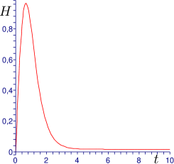
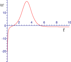
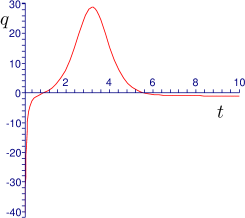
Figure 1: The Hubble parameter $H(t)$, total $w$ and total $q$ for $m_{p}^{2}=0.2$, $a=1$, $p_{20}=1/2$ and $p_{02}=-0.01$

In the case $r<-2$ the $t_{c}$ becomes imaginary and the function $H(t)$ turns out to be monotonic. This situation is close to the one field model. The case $r>0$ is implausible because $H(t)$ changes the sign during the evolution and has a negative asymptotic.

The state parameter $w$ is given by the following expression

$$\begin{split}w=-1+&\frac{4p_{20}m_{p}^{2}}{a^{2}}\cdot\frac{\cosh^{4}(2ap_{20}t)}{p_{02}\cosh^{2}(2ap_{20}t)-p_{02}-3p_{20}}\times\\ \times&\left(\frac{1-3\tanh^{2}(2ap_{20}t)}{\cosh^{2}(2ap_{20}t)-1}+\frac{2p_{02}}{p_{02}\cosh^{2}(2ap_{20}t)-p_{02}-3p_{20}}\right)\end{split}$$ (4.13)

It has a singularity in the origin and behaves as $-1/t^{2}$. At the point $t_{c}$ the state parameter $w$ crosses $-1$ because at this point $\dot{H}(t)=0$. After $t_{c}$ for particular values of the parameters (see Fig. 1) appears a period of deceleration ($q>0$), however, at late times the Universe returns to the acceleration, $w$ and $q$ for this solution approach $-1$ from the above. The latter is evident from the expression for $\Delta$ (3.14)

$$\Delta=-4p_{20}^{2}a^{4}\left(\frac{2+r}{\cosh^{2}(2ap_{20}t)}-\frac{3+r}{\cosh^{4}(2ap_{20}t)}\right).$$

For the large time the first term in the parentheses dominates and since in our case it is assumed that $r>-2$ we obtain that $\Delta<0$, $w$ goes to $-1$ from the above and the solutions have the quintessence like behavior.

4.4 Connection to SSFT

The potential (4.4) contains mass terms for the fields $\phi$ and $\xi$. Their masses are given as follows

$$\begin{split}m_{\phi}^{2}=p_{02}^{2}a^{2}\left(\frac{3a^{2}}{2m_{p}^{2}}-2\right),\\ m_{\xi}^{2}=-2p_{02}p_{20}a^{2}.\end{split}$$ (4.14)

However we have obtained previously the following restrictions: $p_{02}$ should be negative, $p_{20}$ should be positive once the asymptotic $a$ is chosen to be positive in order to have a suitable cosmological behavior. Also it follows from (4.12) that the ratio $r$ should be small if we want to observe a large ratio of the maximal Hubble constant and the asymptotic Hubble constant. These restrictions say us that both $m_{\phi}$ and $m_{\xi}$ are small, the field $\phi$ is a tachyon in the limit of the large reduced Planck mass and the field $\xi$ has a positive mass squared.

The situation drastically changes once we make use of the freedom (4.8). We can choose for simplicity $v_{1}=v_{2}=v_{3}=0$. In this case new potential will give new masses for the fields. Indeed,

$$\begin{split}M_{\phi}^{2}=p_{02}^{2}a^{2}\left(\frac{3a^{2}}{2m_{p}^{2}}-2\right)-4Aa^{2},\\ M_{\xi}^{2}=-2p_{02}p_{20}a^{2}-\frac{4Aa^{2}}{2+r}.\end{split}$$ (4.15)

Provided $p_{02}/A$ is small we effectively change the character of the fields because now if $A>0$ they are both tachyons. Moreover, in the limit $r\to 0$ the ratio of masses $M_{\xi}^{2}/M_{\phi}^{2}$ goes to 2 as it should be if we consider $\phi$ as the open string tachyon and $\xi$ as the closed string tachyon.

The trajectories of fields $\phi$ and $\xi$ are presented in Fig. 2 (red lines).

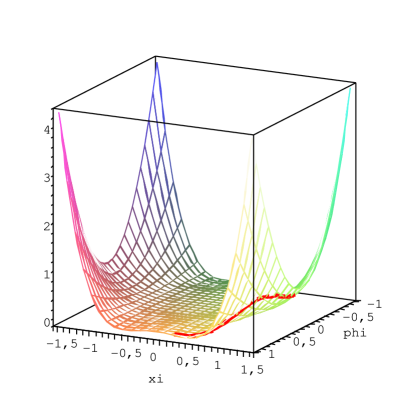
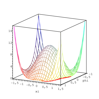
Figure 2: Potential (4.4) for $m_{p}^{2}=0.2$, $a=1$, $p_{20}=1/2$ and $p_{02}=-0.01$ (left) and potential (4.7) for $\rho=\sigma=\tau=0$, $A\alpha=10$ and all other parameters the same as in the left plot (right).

5 Phantom late time solution

5.1 Anzats and corresponding potential

In this section we construct a more involved solution to the system (3.7) which exhibits a phantom like late time behavior for particular values of the parameters. Let us assume the following relations among the coefficients of the system (3.7)

$$p_{02}+x_{02}=-(x_{02}+p_{20})=p_{20}+x_{20}=-c.$$ (5.1)

Under this assumption we have

$$\begin{split}\dot{\phi}(t)&=-p_{02}a^{2}+p_{02}\phi^{2}(t)+2(p_{02}+c)\phi(t)\xi(t)+(p_{02}+2c)\xi^{2}(t),\\ \dot{\xi}(t)&=(p_{02}+c)a^{2}-(p_{02}+c)\phi^{2}(t)-2(p_{02}+2c)\phi(t)\xi(t)-(p_{02}+3c)\xi^{2}(t).\end{split}$$ (5.2)

The superpotential under the conditions (5.1) has the form

$$W=\frac{1}{6m_{p}^{2}}\left(-p_{02}\phi(3a^{2}-\phi^{2})+3(p_{02}+2c)\phi\xi^{2}-3(p_{02}+c)\xi(a^{2}-\phi^{2})+(p_{02}+3c)\xi^{3}\right)$$ (5.3)

and corresponding potential is

$$\begin{split}V&=\frac{1}{2}(-p_{02}a^{2}+p_{02}\phi^{2}+2(p_{02}+c)\phi\xi+(p_{02}+2c)\xi^{2})^{2}-\\ &-\frac{1}{2}((p_{02}+c)a^{2}-(p_{02}+c)\phi^{2}-2(p_{02}+2c)\phi\xi-(p_{02}+3c)\xi^{2})^{2}+\\ &+\frac{1}{12m_{p}^{2}}(p_{02}\phi(3a^{2}-\phi^{2})+3(p_{02}+c)\xi(a^{2}-\phi^{2})-3(p_{02}+2c)\phi\xi^{2}-(p_{02}+3c)\xi^{3})^{2}.\end{split}$$ (5.4)

5.2 Solution

Comparing two lines of the system (5.2) one readily finds

$$\dot{\phi}(t)+\dot{\xi}(t)=ca^{2}-c(\phi(t)+\xi(t))^{2}.$$

Therefore

$$\phi(t)+\xi(t)=a\tanh(ac(t+t_{0})).$$

Substituting $\xi(t)=a\tanh(ac(t+t_{0}))-\phi(t)$ into (5.2) one finds

$$\phi=a\tanh(ac(t+t_{0}))-\frac{a^{2}(p_{02}+c)t-C}{\cosh^{2}(ac(t+t_{0}))}$$ (5.5)

and

$$\xi=\frac{a^{2}(p_{02}+c)t-C}{\cosh^{2}(ac(t+t_{0}))}.$$ (5.6)

A behavior of the solution depends on particular values of parameters $a$, $c$, $t_{0}$ and $C$. We adjust $C$ in such a way that $\phi(0)=0$. This gives

$$C=-\frac{a}{2}\sinh(2act_{0}).$$

The form of trajectories (5.5) and (5.6) for particular values of the parameters is presented in Fig. 3.

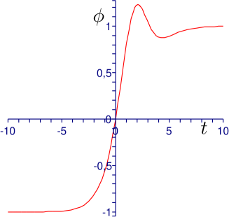
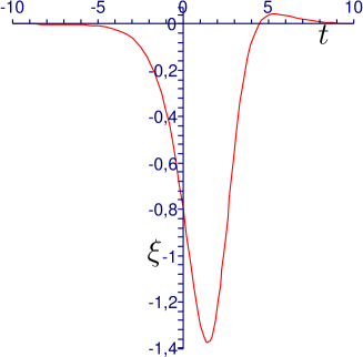
Figure 3: $\phi(t)$ and $\xi(t)$ for $a=1$, $c=0.55$, $p_{02}=-0.05$, $t_{0}=-2$ and $m_{p}^{2}=0.2$.

5.3 Cosmological properties

On solutions (5.5) and (5.6) the Hubble parameter has the following form

$$\begin{split}H(t)&=-\frac{a^{3}p_{02}}{6m_{p}^{2}}\tanh(ac(t+t_{0}))\left(2+\frac{1}{\cosh^{2}(ac(t+t_{0}))}\right)-\\ &-\frac{a^{3}}{4m_{p}^{2}}\frac{2tac(p_{02}+c)+\sinh(2act_{0})}{\cosh^{4}(ac(t+t_{0}))}.\end{split}$$ (5.7)

An analysis of this function is rather involved because we arrive to transcendent equations once we want to find the extrema. The situation is simplified a bit if we use the equation (2.3b) to express the $\dot{H}(t)$. One can write

$$\dot{H}(t)\sim\dot{\phi}^{2}(t)-\dot{\xi}^{2}(t)=(\dot{\phi}(t)-\dot{\xi}(t))(\dot{\phi}(t)+\dot{\xi}(t)).$$

The last multiplier for our solution is equal to

$$\frac{a^{2}c}{\cosh^{2}(ac(t+t_{0}))}.$$

The latter expression has the same sign as $c$ and becomes $0$ only in the infinite future. Note that $c$ should be positive if $a$ is taken to be positive. Otherwise the asymptotic value of $H(t)$ will be negative. Thus, the zeros of the $\dot{H}(t)$ are determined by zeros of the first multiplier $\dot{\phi}(t)-\dot{\xi}(t)$. Also, the sign of the first multiplier can determine the late time behavior. Using exact dependence for the fields one can write

$$\dot{\phi}(t)-\dot{\xi}(t)=a^{2}\frac{2c(2a(p_{02}+c)t+\sinh(2act_{0}))\tanh(ac(t+t_{0}))-c-2p_{02}}{\cosh^{2}(ac(t+t_{0}))}.$$ (5.8)

This expressions leads to the following consequences. The late time behavior is governed by the sign of the sum $p_{02}+c$. It should be positive if we expect the phantom like late time behavior. Also we observe that a natural choice $t_{0}=0$ does not lead to new interesting cosmological properties. Indeed, in this case the expression (5.8) is governed by the function $t\tanh(act)$ which is monotonic at $t>0$. Thus, the nominator of (5.8) has not more than one zero. If so, then we cannot have a large pick for the function $H(t)$ and a phantom like late time behavior simultaneously (exactly such an evolution is interesting from the cosmological point of view) because to posses these properties $H(t)$ should have a local minimum. To summarize we have to have $a>0$, $c>0$, $p_{02}<0$, $t_{0}$ should be finite if we want to observe new effects and $p_{02}+c>0$ for the phantom like late time behavior.

The complete analysis of zeros of the equation (5.8) is very cumbersome. However, it is possible to find particular values of the parameters for which it has two roots. This situation is demonstrated in Fig. (4).

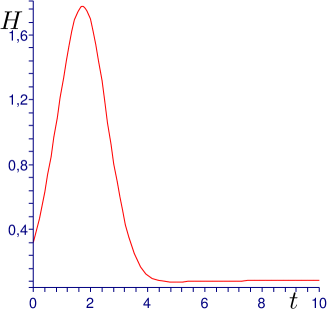
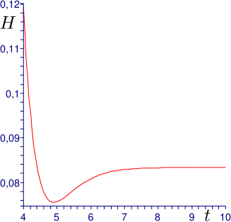
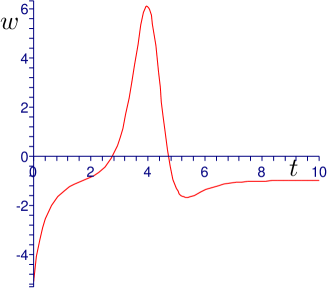
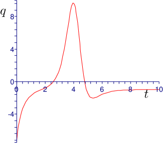
Figure 4: The Hubble parameter $H(t)$ and its fine structure (top pictures). The state parameter $w(t)$ and deceleration parameter $q(t)$ (bottom pictures). Here $a=1$, $c=0.55$, $p_{02}=-0.05$, $t_{0}=-2$ and $m_{p}^{2}=0.2$.

6 Conclusion and Discussion

In this paper we have investigated the dynamics of two component DE models, with one phantom field and one usual field with special polynomial potentials. The main motivation for us was a model of the the Universe as a slowly decaying D3-brane which dynamics is described by a tachyon field [6]. To take into account the back reaction of gravity we take one more scalar field. This scalar field has usual kinetic term. The model is close to the model considered by [23] which is also considered in the DE context. Note also that in the closed bosonic string sector an extra phantom appears [24]. Within two component DE models with a general class of interactions which correspond to polynomial superpotentials we have found restrictions that show whether the model is a phantom-like ($w$ goes to -1 from below), or it is a quintessence-like ($w$ goes to -1 from above).

In particular, for the simplest model inspired by a D3-brane we have found that an inclusion of the closed string tachyon drastically changes the late time regime and for two-component model $w>-1$ at large time, while in open string case $w<-1$ at large time.

The model considered in this paper is close to the model considered in [23]. This model is unstable, while a stability of our model is provided by its string origin. Note also that in the closed bosonic string sector appears an extra phantom [24].

The two-component model considered in this paper is interesting also by the following reason. There are several attempts to unify the early time inflation with late time accelerated universe (see for example [25] and refs. therein). Generally speaking it is rather difficult to do this mainly because the ratio of the Hubble parameters in the end of inflation to its value during the period of the late acceleration should be very large. In our case we have such a possibility just by taking $r$ to be close to $0$ in formula (4.12).

Let us recall that two scalar fields, both with usual kinetic terms, have been used in the hybrid inflation [26], and in particular in [27] the superpotential has a simple quadratic form.

We have also found the superpotentials depending on two components for which $w<-1$ at late times. We have presented the explicit solution realizing this possibility. It would be very interesting to study small deformations of the corresponding potential and to make clear does the constructed solution stable or not under deformations of the form of potentials and after including the CDM.

References

- [1] A.G. Riess et al., Observational Evidence from Supernovae for an Accelerating Universe and a Cosmological Constant, Astron. J. 116 (1998) 1009, astro-ph/9805201.
- [2] S.J. Perlmutter et al., Measurements of Omega and Lambda from 42 High-Redshift Supernovae, Astroph. J. 517 (1999) 565, astro-ph/9812133.
- [3] D.N. Spergel et al., First Year Wilkinson Microwave Anisotropy Probe (WMAP) Observations: Determination of Cosmological Parameters, Astroph. J. Suppl. 148 (2003) 175, astro-ph/0302209.
- [4] J.L. Tonry et al., Cosmological Results from High-z Supernovae, Astrophys. J. 594 (2003) 1–24, astro-ph/0305008. M. Tegmark at al., Cosmological parameters from SDSS and WMAP, Phys. Rev. D69 (2004) 103501, astro-ph/0310723. A.G. Riess, et al., Type Ia Supernova Discoveries at From the Hubble Space Telescope: Evidence for Past Deceleration and Constraints on Dark Energy Evolution, Astroph. J. 607 (2004) 665–687, astro-ph/0402512. U. Seljak at al., Cosmological parameter analysis including SDSS Ly-alpha forest and galaxy bias: constraints on the primordial spectrum of fluctuations, neutrino mass, and dark energy, aspto-ph/0407372. M.Tegmark, What does inflation really predict?, JCAP 0504 (2005) 001, astro-ph/0410281.
- [5] R.R. Caldwell, Dark Energy, Physics World, 17, No. 5 (2004) 37. R.R. Caldwell, A Phantom Menace? Cosmological consequences of a dark energy component with super-negative equation of state, Phys. Lett. B545 (2002) 23, astro-ph/9908168. R.R. Caldwell, M. Kamionkowski, N.N. Weinberg, Phantom Energy and Cosmic Doomsday, Phys. Rev. Lett. 91 (2003) 071301, astro-ph/0302506. S.M. Carroll, M. Hoffman, M. Trodden, Can the dark energy equation-of-state parameter be less than -1?, Phys. Rev. D68 (2003) 023509, astro-ph/0301273. J.M. Cline, S. Jeon, G.D. Moore, The phantom menaced: constraints on low-energy effective ghosts, Phys. Rev. D70 (2004) 043543, hep-ph/0311312. B. McInnes, The dS/CFT Correspondence and the Big Smash, JHEP 0208 (2002) 029, hep-th/0112066. B. McInnes, What if ?, in: ”On the Nature of Dark Energy: Proceedings of the XVIIIth Colloquium of the Institut d’Astrophysique de Paris, July 2002”, Edited by P. Brax, J. Martin, J.P. Uzan., p. 265, astro-ph/0210321. S. Nesseris, L. Perivolaropoulos, The Fate of Bound Systems in Phantom and Quintessence Cosmologies, Phys. Rev. D70 (2004) 123529, astro-ph/0410309 S.D.H. Hsu, A. Jenkins, M.B. Wise, Gradient instability for , Phys. Lett. B597 (2004) 270–274, astro-ph/0406043. V.K. Onemli, R.P. Woodard, Super-Acceleration from Massless, Minimally Coupled , Class. Quant. Grav. 19 (2002) 4607, gr-qc/0204065; V.K. Onemli, R.P. Woodard, Quantum effects can render on cosmological scales, Phys. Rev. D70 (2004) 107301, gr-qc/0406098. A.A. Starobinsky, Future and Origin of our Universe: Modern View, Grav. Cosmol. 6 (2000) 157–163, astro-ph/9912054. U. Alam, V. Sahni, T.D. Saini, A.A. Starobinsky, Is there Supernova Evidence for Dark Energy Metamorphosis?, Mon.Not.Roy.Astron.Soc. 354 (2004) 275, astro-ph/0311364. U. Alam, V. Sahni, A.A. Starobinsky, The case for dynamical dark energy revisited, JCAP 0406 (2004) 008, astro-ph/0403687. C. Csaki, N. Kaloper, J. Terning, Exorcising , Annals Phys. 317 (2005) 410–422, astro-ph/0409596 T. Padmanabhan, Accelerated expansion of the universe driven by tachyonic matter, Phys. Rev. D66 (2002) 021301, hep-th/0204150. T. Padmanabhan, T. Roy Choudhury, Can the clustered dark matter and the smooth dark energy arise from the same scalar field ?, Phys.Rev. D66 (2002) 081301, hep-th/0205055. A. Melchiorri, L. Mersini, C.J. Odman, M. Trodden, The State of the Dark Energy Equation of State, Phys. Rev. D68 (2003) 043509, astro-ph/0211522. Bo Feng, Xiulian Wang, Xinmin Zhang, Dark Energy Constraints from the Cosmic Age and Supernova, astro-ph/0404224. Bo Feng, Mingzhe Li, Yun-Song Piao, Xinmin Zhang, Oscillating Quintom and the Recurrent Universe, astro-ph/0407432. S. Nojiri, S. Odintsov, The final state and thermodynamics of dark energy universe, hep-th/0408170. W. Fang, H.Q. Lu, Z.G. Huang, K.F. Zhang, Phantom Cosmology with Born-Infeld Type Scalar Field, hep-th/0409080. Jian-gang Hao, Xin-zhou Li, Attractor Solution of Phantom Field, Phys. Rev. D67 (2003) 107303, gr-qc/0302100. P. Singh, M. Sami, N. Dadhich, Cosmological Dynamics of Phantom Field, Phys. Rev. D68 (2003) 023522, hep-th/0305110. Rong-Gen Cai, Anzhong Wang, Cosmology with Interaction between Phantom Dark Energy and Dark Matter and the Coincidence Problem, hep-th/0411025. Zong-Kuan Guo, Yuan-Zhong Zhang, Interacting Phantom Energy, astro-ph/0411524. S.M. Carroll, A. de Felice, M. Trodden, Can we be tricked into thinking that is less than -1?, astro-ph/0408081.
- [6] I.Ya. Aref’eva, Nonlocal String Tachyon as a Model for Cosmological Dark Energy, astro-ph/0410443.
- [7] I.Ya. Aref’eva, A.S. Koshelev, S.Yu. Vernov, Exactly solvable SFT insipred phantom model, astro-ph/0412619.
- [8] A. Vikman, Can dark energy evolve to the Phantom?, Phys. Rev. D71 (2005) 023515, astro-ph/0407107.
- [9] I.Ya. Aref’eva, A.S. Koshelev, S.Yu. Vernov, Stringy Dark Energy Model with Cold Dark Matter, astro-ph/0505605.
- [10] B. Boisseau, G. Esposito-Farese, D. Polarski, A.A. Starobinsky, Reconstruction of a scalar-tensor theory of gravity in an accelerating universe, Phys. Rev. Lett. 85 (2000) 2236, gr-qc/0001066. V. Sahni, Yu.V. Shtanov, Braneworld models of dark energy, JCAP 0311 (2003) 014, astro-ph/0202346. B. McInnes, The Phantom Divide in String Gas Cosmology, Nucl.Phys. B718 (2005) 55–82, hep-th/0502209. L. Perivolaropoulos, Constraints on linear-negative potentials in quintessence and phantom models from recent supernova data, Phys. Rev. D71, 063503 (2005), astro-ph/0412308; L. Perivolaroupoulos, Reconstruction of Extended quintessence potentials from the SnIa Gold Dataset, astro-ph/0504582. Bo Feng, Xiulian Wang, Xinmin Zhang, Dark Energy Constraints from the Cosmic Age and Supernova, Phys.Lett. B607 (2005) 35–41, astro-ph/0404224 Zong-Kuan Guo, Yun-Song Piao, Xinmin Zhang, Yuan-Zhong Zhang, Cosmological Evolution of a Quintom Model of Dark Energy, Phys.Lett. B608 (2005) 177–182, astro-ph/0410654 R.R. Caldwell, M. Doran, Dark-Energy Evolution Across the Cosmological-Constant Boundary, astro-ph/0501104. Hao Wei, Rong-Gen Cai, Ding-Fang Zeng, Hessence: A New View of Quintom Dark Energy, hep-th/0501160. Xiao-Fei Zhang, Hong Li, Yun-Song Piao, Two-field models of dark energy with equation of state across -1, astro-ph/0501652. Ming-zhe Li, Bo Feng, Xin-min Zhang, A single scalar field model of dark energy with equation of state crossing -1, hep-ph/0503268. M. Sami, A. Toporensky, P.V. Tretjakov, Sh. Tsujikawa, The fate of (phantom) dark energy universe with string curvature corrections, Phys. Lett. B619 (2005) 193, hep-th/0504154. Hrvoje Stefancic, Dark energy transition between quintessence and phantom regimes — an equation of state analysis, astro-ph/0504518. A. Anisimov, E. Babichev, A. Vikman, B-Inflation, JCAP 0506 (2005) 006, astro-ph/0504560. A.A. Andrianov, F. Cannata, A.Y. Kamenshchik, Smooth dynamical (de)-phantomization of a scalar field in simple cosmological models, gr-qc/0505087. L.P. Chimento, D. Pavon, Dual interacting cosmologies and the coincidence problem, gr-qc/0505096. Rong-Gen Cai, Hong-Sheng Zhang, Anzhong Wang, Crossing in Gauss-Bonnet Brane World with Induced Gravity, hep-th/0505186. Sh. Nojiri, S.D. Odintsov, Inhomogeneous equation of state of the universe: phantom era, future singularity and crossing the phantom barrier, hep-th/0505215.
- [11] E. Witten, Noncommutative geometry and string field theory, Nucl. Phys. B268 (1986) 253; E. Witten, Interacting field theory of open superstrings, Nucl.Phys. B276 (1986) 291.
- [12] I.Ya. Aref’eva, P.B. Medvedev, A.P. Zubarev, Background formalism for superstring field theory, Phys.Lett. B240 (1990) 356; C.R. Preitschopf, C.B. Thorn, S.A. Yost, Superstring Field Theory, Nucl.Phys. B337 (1990) 363; I.Ya. Aref’eva, P.B. Medvedev, A.P. Zubarev, New representation for string field solves the consistency problem for open superstring field, Nucl.Phys. B341 (1990) 464;
- [13] N. Berkovits, A. Sen, B. Zwiebach, Tachyon Condensation in Superstring Field Theory, Nucl.Phys. B587 (2000) 147–178, hep-th/0002211.
- [14] I.Ya. Arefeva, D.M. Belov, A.S. Koshelev, P.B. Medvedev, Tahyon Condensation in the Cubic Superstring Field Theory, Nucl.Phys B, 638 ( 2002) 3–20, hep-th/0011117; Gauge Invariance and Tahyon Condensation in the Cubic Superstring Field Theory, Nucl.Phys B 638 (2002) 21–40, hep-th/0107197.
- [15] K. Ohmori, A Review on Tachyon Condensation in Open String Field Theories, hep-th/0102085; I.Ya. Aref’eva, D.M. Belov, A.A. Giryavets, A.S. Koshelev, P.B. Medvedev, Noncommutative Field Theories and (Super)String Field Theories, hep-th/0111208; W. Taylor, Lectures on D-branes, tachyon condensation and string field theory, hep-th/0301094.
- [16] Ya.I. Volovich, Numerical study of Nonlinear Equations with Infinite Number of Derivatives, J.Phys. A36 (2003) 8685–8702, math-ph/0301028. V.S. Vladimirov, Ya.I. Volovich, Nonlinear Dynamics Equation in p-Adic String Theory, Theor. Math. Phys., 138 (2004) 297–309, math-ph/0306018.
- [17] I.Ya. Aref’eva, L.V. Joukovskaya, A.S. Koshelev, Time Evolution in Superstring Field Theory on non-BPS brane. Rolling Tachyon and Energy-Momentum Conservation, hep-th/0301137. I.Ya. Aref’eva, Rolling tachyon in NS string field theory, Fortschr. Phys. 51 (2003) 652. I.Ya. Aref’eva, L.V. Joukovskaya, Rolling Tachyon on non-BPS brane, Lectures given at the II Summer School in Modern Mathematical Physics, Kopaonik, Serbia, 1–12 Sept. 2002.
- [18] K. Ohmori, Toward open closed string theoretical description of rolling tachyon. Phys.Rev. D69 (2004) 026008, hep-th/0306096.
- [19] L.V. Joukovskaya, Ya.I. Volovich, Energy Flow from Open to Closed Strings in a Toy Model of Rolling Tachyon, math-ph/0308034.
- [20] B. Zwiebach, Oriented open - closed string theory revisited. Annals Phys. 267 (1998) 193–248, hep-th/9705241.
- [21] I.Ya. Aref’eva, L.V. Joukovskaya, Time Lumps in Nonlocal Stringy Models and Cosmological Applications, hep-th/0504200.
- [22] O. DeWolfe, D.Z. Freedman, S.S. Gubser, A. Karch, Modeling the fifth dimension with scalars and gravity, Phys. Rev. D62 (2000) 046008, hep-th/9909134.
- [23] S.M. Carroll, M. Hoffman, M. Trodden, Can the dark energy equation-of-state parameter w be less than -1? , Phys.Rev. D68 (2003) 023509, astro-ph/0301273.
- [24] H. Yang, B. Zwiebach, Rolling Closed String Tachyons and the Big Crunch, hep-th/0506076.
- [25] E.J. Copeland, M.R. Garousi, M. Sami, S. Tsujikawa, What is needed of a tachyon if it is to be the dark energy?, Phys.Rev. D71 (2005) 043003, hep-th/0411192. Sh. Nojiri, S.D. Odintsov, Unifying phantom inflation with late-time acceleration: scalar phantom-non-phantom transition model and generalized holographic dark energy, hep-th/0506212. Sh. Nojiri, S.D. Odintsov, Phys. Lett. B562 (2003) 147, Quantum deSitter cosmology and phantom matter hep-th/0303117; Effective equation of state and energy conditions in phantom/tachyon inflationary cosmology perturbed by quantum effects, Phys.Lett. B571 (2003) 1, hep-th/0306212.
- [26] A. Linde, Hybrid Inflation, Phys.Rev. D49 (1994) 748–754, astro-ph/9307002.
- [27] E.L. Copeland, A.R. Liddle, D.H. Lyth, E.D. Stewart, D. Wands, False Vacuum Inflation with Einstein Gravity, Phys.Rev. D49 (1994) 6410–6433, astro-ph/9401011; G.R. Dvali, Q. Shafi, R.K. Schaefer, Large Scale Structure and Supersymmetric Inflation without Fine Tuning, Phys.Rev.Lett. 73 (1994) 1886–1889, hep-ph/9406319