Point Source Extraction with MOPEX

Abstract

MOPEX (MOsaicking and Point source EXtraction) is a package developed at the Spitzer Science Center for astronomical image processing. We report on the point source extraction capabilities of MOPEX. Point source extraction is implemented as a two step process: point source detection and profile fitting. Non-linear matched filtering of input images can be performed optionally to increase the signal-to-noise ratio and improve detection of faint point sources. Point Response Function (PRF) fitting of point sources produces the final point source list which includes the fluxes and improved positions of the point sources, along with other parameters characterizing the fit. Passive and active deblending allows for successful fitting of confused point sources. Aperture photometry can also be computed for every extracted point source for an unlimited number of aperture sizes. PRF is estimated directly from the input images. Implementation of efficient methods of background and noise estimation, and modified Simplex algorithm contribute to the computational efficiency of MOPEX. The package is implemented as a loosely connected set of perl scripts, where each script runs a number of modules written in C/C++. Input parameter setting is done through namelists, ASCII configuration files. We present applications of point source extraction to the mosaic images taken at 24 and 70 $\mu$m with the Multiband Imaging Photometer (MIPS) as part of the Spitzer extragalactic First Look Survey and to a Digital Sky Survey image. Completeness and reliability of point source extraction is computed using simulated data.

1 Introduction

Detection of point sources and estimation of their coordinates, fluxes and other pertinent parameters from celestial images is a continuing challenge in modern astronomy. A number of packages performing point source extraction has been developed, among them SExtractor (Bertin & Arnouts, 1996), StarFinder (Diolaiti et al., 2000), DAOPHOT (Stetson, 1987), and DoPHOT (Schechter et al., 1993).

Due to the specific nature of Spitzer data and the data collection strategy there was a need to develop a point source extractor that would combine the best features of existing programs and extend their capabilities. Spitzer data range from undersampled IRAC (InfraRed Array Camera) data with very low background to high background nearly Nyquist-sampled low noise MIPS24 (Multiband Imaging Photometer at 24 $\micron$) data or very noisy MIPS70 (Multiband Imaging Photometer at 70 $\micron$) data. Also for each instrument different observing strategies result in images that are background limited or confusion limited. The point source extractor has to be very flexible to accomodate this variety of data.

MOPEX has been designed to be applicable in all these cases. Point source extraction is implemented as a two step process: point source detection and profile fitting. MOPEX has two modes of point source extraction - single frame and multiframe. In the single frame mode point source detection and subsequent fitting is performed in the same image. In the multiframe mode point source extraction is performed in a set of input frames. However, the detection is performed in the mosaic image created by combining the set of input frames into a single mosaic image. The signal-to-noise ratio is higher in a mosaic image and this fact justifies performing detection there. Since mosaicking is part of MOPEX(Makovoz & Khan, 2004), point source extraction benefits from such capabilities as creating properly resampled mosaic images, cosmic ray hits masking, etc. The difference between the single frame and multiframe modes is the way the point source fitting is performed. In the multiframe mode it is done simultaneously in all the input frames. The mosaic mode of operation is better suited for well sampled data where one can obtain a good estimate of PRF in the mosaic image. Also one should use the mosaic mode for data with high depth of coverage, since simultaneous point source fitting in a great number of images becomes computationally prohibitive.

Point source fitting requires a point response function (PRF). MOPEX can use a PRF produced by some outside means, but for better performance the PRF should be estimated from the data itself. MOPEX has such capabilities. The package provides means of estimating PRF for both single and multiframe point source extraction modes.

This paper deals with the single frame (mosaic) mode of point source extraction and PRF estimation. Description of the multiframe mode of MOPEX will be given elsewhere. The structure of this paper is as follows. In Section 2 we give an overview of the processing in the mosaic mode. Background subtraction and noise estimation are described in Section 3. In Section 4 we describe the non-linear matched filtering technique used to enhance point sources. We also give a short description of the image segmentation. In Section 5 we describe the point source fitting performed using a modified Simplex algorithm. Passive and active deblending are also discussed there. Section 6 is a brief description of PRF estimation in a mosaic image. In Section 7 we present applications of MOPEX to two Spitzer mosaic images and to a Digital Sky Survey (DSS) image. In Section 8 we present the results of validating MOPEX with simulated data. Appealing features of MOPEX are processing speed and photometric accuracy. See Section 8.1 for the timing results of MOPEX.

2 Processing Overview

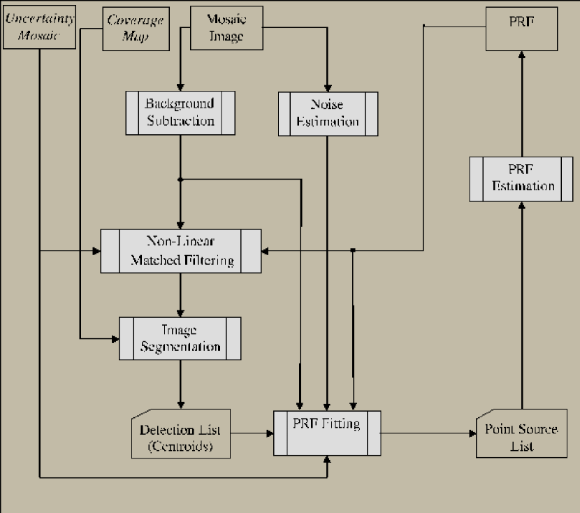
Figure 1: Point source extraction processing chain. The gray boxes represent the processing steps and the white boxes represent the data. Optional input is italicized.

The mosaic mode of operation is shown in Figure 1. In addition to the mosaic image there are two optional input images: the coverage map and uncertainty image. The coverage map gives the number of input frames that were combined to produce each mosaic pixel. The uncertainty image gives the uncertainty for each input image pixel. These two images are created when mosaicking is done with MOPEX. They are used at a various stages in the point extraction process. The coverage map is used in point source detection. The uncertainty image is used for filtering and point source fitting. Normally, Spitzer data come with uncertainty images from which a mosaic of uncertainty images can be created. If no uncertainty images exist they can be estimated by MOPEX using the model consisting of three components - photon noise, read noise, and confusion noise.

Important steps in the processing are creating background subtracted and noise images. Background subtraction is done by computing the median and subtracting it. The background subtracted image is used as an input for the filtering as well as point source fitting. The noise image is produced for the purpose of computing the signal-to-noise ratio (SNR) of the point sources. Optionally, this noise image can be used instead of the uncertainty image, if the latter is not avalaible and can not be reliably computed. An efficient sliding window technique is implemented for computing both products.

For better results filtering is done as a preliminary step before image segmentation. Filtering can be a simple median subtraction or a more complicated non-linear matched filtering producing a point source probability image. Non-linear matched filtering significantly increases the SNR of the point sources in the filtered image and also supresses contribution of cosmic ray hits and various artifacts. Only in rare cases of images with very low, almost negligible, noise level and high point source density using the product of the non-linear filtering for image segmentation can be detrimental.

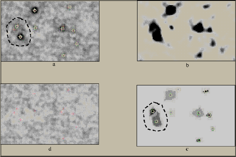
Figure 2: A small fragment (90 by 60 pixels) of MIPS70 mosaic shown in Figure 7 is used to illustrate the products of the processing chain. a) Input image with the detections shown as white circles, and final extractions shown as white crosses. An example of active deblending is circled with the black dashed line. b) Point source probability image. c) Detection map with the detections shown as white circles. An example of a blend with $N_{p}$ = 2 is circled with a black dashed line. The white dashed line circles the detection that was discarded because of its small size. d) Point source subtracted image.

The result of image segmentation is the detection list with the positions of candidate point source are determined. During the estimation stage a thorough fit of the data is performed to refine the positions, determine the fluxes and deblend extracted point sources. The background subtracted image is normally used for the point source fitting. A point source subtracted image can be produced to assess the quality of point source extraction. A point response function (PRF) is required to perform linear matched filtering and data fitting. MOPEX included a separate task of PRF estimation. We illustrate the intermediate products at various processing stages in Figure 2 using a small fragment (90 by 60 pixels) of an MIPS70 mosaic image. The mosaic is described in more details in Section 7.2.

In this paper we present an overview of the algorithm. One can create a custom-tailored processing chain to accomodate for any specific features of the data, as descrived, for example, in Section 7.1. Careful tuning of various stages can be performed using a number of parameters. For details on running MOPEX, comprehensive listing of all the processing parameters, and sample namelists one can consult the online guide .

3 Background and Noise Estimation

Background subtracted images are used for both point source detection and fitting. A common way of estimating the background is to find for each pixel the median in a window centered around that pixel. This method will inevitably overestimate the background in the vicinity of bright sources. MOPEX provides a user controlled way to alleviate the bias introduced by the bright sources. One can counter-bias the median by excluding a fixed number of pixels with highest values in each window from median computation, thus offsetting the bias introduced by the presence of bright sources. This number is defined by the user and is constant througout the image to which it is applied. This step may require further optimization by automatically adjusting this number based on the crowdiness in any particular window. However, even in its present state the quality of median subtracted images satisfies the needs of point source detection. Any bias in the background estimation introduced by the median filtering can be corrected at the point source fitting stage as described below in Section  5, since the fitting includes among other fitting parameters a constant background for the fitting area.

By increasing the window size one can decrease the fluctuations in the number of point sources per window and in general get a more robust estimate of the median. The problem with increasing the window size is the corresponding increase of the processing time. In order to find the median the values of the pixels in the window should be sorted. If sorting is done from scratch for each window this process becomes prohibitively slow. To speed up the process and make median filtering practical for relatively big windows, we use the sliding window approach. The pixel values are sorted in the first window which is located in a corner of the image. Subsequently, as the window slides by one column the pixels from the dropped out column are removed from the sorted list of pixels and the new column is inserted in the sorted list of pixels. Various data structures have been used for fast median computation (see Juhola et al. (1991) and references therein). We implemented a variant of the binary search tree method. This approach significantly speeds up the processing. The processing time scales with the linear size of the sliding window, whereas if the sorting is performed from scratch in each window the processing time scales at least as the area of the window. On a 1 GHz Sparc Sun workstation processing time for computing the median for a window of size 100x100 pixels is $10^{-4}$ sec/per pixel.

Noise images are used for computing the SNR of the point sources. Noise images for each pixel give a value of background fluctuation in a window centered on the pixel. They are computed based on the assumption of Gaussian distribution of pixel values around the underlying sky value. The presence of point sources results in broadening of the pixel distribution and overestimation of the noise level. Just like in the background estimation this can be alleviated by excluding the highest pixel values in each window. Noise estimation is an extension of median filtering. The median pixel $i_{med}$ is found for each window. Then the noise value $n$ is determined as

$$n=(w[i_{med}+0.34W]-w[i_{med}-0.34W])/2.$$ (1)

Here $w$ is the sorted array of pixels in the window, $W$ is the size of the array. The same sliding window technique is used here as in background estimation.

4 Point Source Detection

Point source detection is performed either on background subtracted images, or optionally additional filtering can be performed.

4.1 Non-linear Matched Filtering

The purpose of filtering is to reduce fluctuations of the background noise and to enhance point source contributions. It is a common practice to perform linear matched filtering to reach the above goals (Andrews, 1970). A matched filter can be derived (Cook & Bernfeld, 1970) on the basis of optimizing SNR, likelihood ratio, or mean square error (MSE). Standard derivation of linear matched filter involves an assumption of either a single point source or the Gaussian distribution of the point sources. In reality the distribution function of point sources is highly non-Gaussian. Under such condition the linear filter becomes sub-optimal and the optimal filter is non-linear. The general form of a such a filter is very complicated  (Makovoz, 2005) and its derivation involves fitting the point source distribution function with the Gaussian mixture model. Application of such a filter is computation-intensive. For practical purposes we take the general idea of non-linear filtering and derive a non-linear filter based on the notion of point source probability. The details of the derivation are given in Appendix A. A point source probability image is computed as follows:

$$PSP(j)=(1+\frac{(1-Pr)\sigma_{x}}{Pr\sigma_{T}}exp(-\frac{(\sum_{i}s(i)PRF(i))^{2}}{2\sigma_{n}^{4}/\sigma_{T}^{2}}))^{-1},$$ (2)

where $s(i)$ is the pixel value of the input image, $PSP(j)$ is the value of pixel $j$ in the point source probability image and $Pr$ is an apriori probability of point source presence. Quantities $\sigma_{x}$, $\sigma_{n}$, and $\sigma_{T}$ are defined in Appendix A. The algorithm is not sensitive to the exact value of $Pr$ which is set by default to 0.1. Figure 2b shows the $PSP$ image corresponding to the input image in Figure 2a. Convolution with the PRF causes some smearing of the point sources. The smearing, however, is not of concern, since the filtered images are used for detection only.

4.2 Image Segmentation

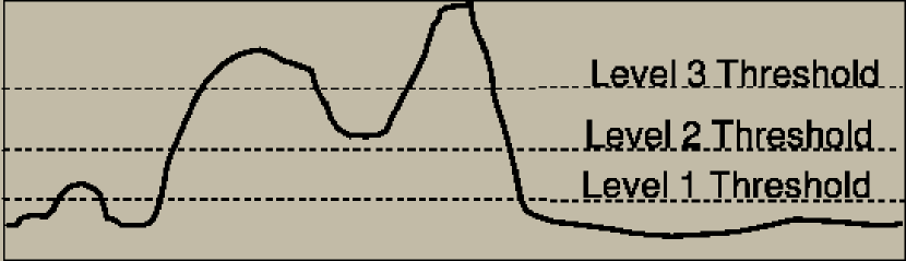
Figure 3: Shown here is a cross-section of an image being segmented. Pixels with the values higher than a segmentation threshold are grouped into contiguous clusters. The segmentation threshold is raised in order to reduce the sizes of the detected clusters of pixels.

Filtered images undergo a process of image segmentation. Contiguous clusters of pixels with the values greater than a user-specified threshold are identified. If the number of pixels in a cluster is smaller than a user-specified threshold, the cluster is rejected. This procedure serves as an additional guard against cosmic rays affected pixels and peaks in background noise fluctuations. If the number of pixels is greater than a user-specified threshold, the cluster is subjected to further segmentation with a higher threshold (Figure 3).

The process of raising threshold is very sensitive. Initially the threshold $T$ defined in terms of a robust estimate of the background fluctuations in the filtered image. The subsequent increase of the threshold is is the essential part of passive de-blending as described below in Section 5.1. The simple approach implemented in MOPEX is as follows. For each cluster a new value of the threshold is found based on the mean pixel value and the standard deviation of the pixel values in the cluster. The drawback of such approach is that it misses a lot of sources which are close to brigher sources. It the original clusters contains one bright and several faint sources the raised threshold will miss the faint sources.

A more complicated scheme has been implemented to facilitate passive de-blending. This scheme uses the concept of peak pixels. A pixel is declared a peak pixel it its value is greater than the values of a user specified number of adjacent pixels. In this scheme the cluster is split as long as there are more than one peak pixel in it. The minimum peak pixel value in the cluster $P_{min}$ is determined. The effective segmentation threshold $T_{n}$ for the detection level $l$ is equal to

$$T_{n}=P_{min}-\frac{T}{l}.$$ (3)

This scheme ensures that no faint sources are missed in the presence of a bright neigbor.

The program keeps track of threshold raising and assigns a detection level to each pixel based on the last threshold value for which this pixel was above the threshold. The original threshold corresponds to the detection level 1. Each time the threshold is raised the detection level is incremented. A detection map image can be created to visualize the image segmentation process. Figure 2c shows the detection map corresponding to the input image in Figure 2a. It has an example of a detection that was discarded because its size was smaller than the user-specified threshold; it is circled with the white dashed line. Higher levels of detection are shown with darker shades of gray. When the process of segmentation is finished the centroids of the clusters are calculated and stored in the detection list (see Figure 1.) Centroids that belong to the same first level detection clusters are marked in the detection table as part of the same blend. The size of the blend defines the initial $N_{p}$ for point source fitting below in equation 4. An example of such a blend with $N_{p}=2$ is circled in Figure 2c with a black dashed line.

Mosaic images in general have variable coverage. Applying a constant pixel value threshold results in variable effective threshold; areas of higher coverage will have higher threshold in terms of the SNR of the detected point sources. To overcome this problem the coverage map is used to attenuate the image undergoing segmentation. The input image is multiplied by the square root of the coverage before it undergoes the process of segmentation. It can be done for any input image, i.e. either the background subtracted image or the probability map. Also, optionally one can specify minimum coverage to prevent detections in the areas of low coverage, which are usually very noisy and where detection can not be performed reliably even after the filtering is performed.

5 Point Source Fitting

Final point source position and photometry estimation is performed for all detections on the detection list. For each point source candidate the data in the input image is fit with the PRF. Fitting is performed by minimizing $\chi^{2}$:

$$\chi^{2}=\sum_{i\in W}\frac{(s(i)-\sum_{n=1}^{N_{p}}f_{n}PRF(i,{\mathbf{R}}_{n})-b)^{2}}{\sigma^{2}(i)}.$$ (4)

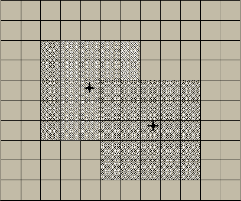
Figure 4: Fitting area for simultaneous fitting of two point sources. The detection positions are shown with black crosses. Each detection has a fitting area of a 5 $\times$ 5 pixels square.

Here the summation is performed over pixels $i$ from the fitting area $W$; $s(i)$ and $\sigma(i)$ are the pixel values of the input image and uncertainty image, correspondingly; $f_{n}$ and ${\mathbf{R}}_{n}$ are the flux and the position of the $n-th$ point source; $PRF(i,{\mathbf{R}}_{n}$) is the contribution of the $n-th$ point source to the $i-th$ pixel; $b$ is the constant background within the fitting area that can be used in this formula optionally. The number $N_{p}$ of point sources fit simultaneously is set to 1 initially if the detection does not belong to a blend, as described in the previous section. For the detections belonging to a blend the number $N_{p}$ is initially set to the size of the blend. PRF contribution is computed for any fractional position of the point source; a bilinear interpolation is performed from the grid points available in the PRF. The fitting area $W$ is a combination of rectangle areas centered on the detection positions (Figure  4). The size of each rectangle is specified by the user and should be set to be on the order of the size of the Airy disk. If set properly, the fitting areas of the point sources belonging to one blend are partially overlapping. As a result of detection point sources with the overlapping contributions should belong to one blend. However, if the detection is done poorly, e.g. if the detection threshold is set too high, then such sources will be erroneously put in two separate blends and not fit simultaneously. If the uncertainty image is not available, the noise image can used instead. Users have an option of using the background subtracted mosaic, using the original image and fitting the background for each point source, or doing both.

The strategy used for minimization of $\chi^{2}$ is a hybrid of a modified simplex algorithm and the gradient descent algorithm. The simplex algorithm does not use derivatives of the functions involved in minimization. It is a desirable feature since the world coordinate transformations are very complicated functions of their arguments. We made several modifications of the algorithm, which are described in Appendix B. Simplex operations are applied to the point sources positions. On the other hand the derivatives with respect to the fluxes of the point sources and the background are taken easily:

$$\frac{\partial\chi^{2}}{\partial f_{k}}=-2\sum_{i\in W}\frac{PRF(i,{\mathbf{R}}_{k})(s(i)-\sum_{n=1}^{N_{p}}f_{n}PRF(i,{\mathbf{R}}_{n})-b)}{\sigma^{2}(i)};$$

$$\frac{\partial\chi^{2}}{\partial b}=-2\sum_{i\in W}\frac{(s(i)-\sum_{n=1}^{N_{p}}f_{n}PRF(i,{\mathbf{R}}_{n})-b)}{\sigma^{2}(i)};$$ (5)

and that justifies the choice of the gradient descent method for the fluxes and the background.

In general, several point sources are used to fit the data simultaneously as explained in the next section. A $2-$dimensional simplex is constructed for the position vector of each point source. The appropriate simplex operations is performed for each point source separately. After the positions of the point sources are adjusted each flux and the background are adjusted along the gradient given by the equation 5. The procedure is repeated until one of the stopping criteria specified below is met. Since each simplex is moved separately, it reduces the complexity of the algorithm. The reflections, etc. are performed in the $2-$dimensional space of the position vertor for each point source, as opposed to the $2N_{p}$ dimensional space of the vector describing the position of all $N_{p}$ sources.

The goodness-of-fit is assessed by the values of $\chi^{2}/dof$. The number of the degrees of freedom $dof$ is equal to the size of the fitting area $W$ minus the number of the fitting parameters, which is 3 per point source and one for the background, if it is used in the minimization. The program attempts to minimize $\chi^{2}/dof$ to be below the user specified threshold. If the number of iterations exceeds the limit or the relative change of $\chi^{2}$ drops below the limit, fitting terminates, even though the $\chi^{2}$ is still greater than the threshold.

5.1 Passive and Active Deblending

If several point sources are within the reach of each others PRF’s they should be fit simultaneously. This is done if $N_{p}>1$ in equation 4. This process is known as point source deblending. There are two mechanisms in MOPEX to perform deblending.

The first one is called passive deblending. The point sources identified at the detection stage as belonging to one blend are fit simultaneously. In this case fitting starts with the value $N_{p}>1$.

The second mechanism is called active deblending. During active deblending $N_{p}$ is incremented during the fitting process. If $\chi^{2}/dof$ for a point source is above the user specified threshold, the algorithm increments $N_{p}$ and fits the same data with more point sources. If the improvement in $\chi^{2}/dof$ is significant, then the additional point source is accepted. Otherwise the algorithm reverts to the previous solution. In case of succesful active deblending if $\chi^{2}/dof$ is still greater than the threshold, active deblending continues untill the program reaches the user defined limit on $N_{p}$.

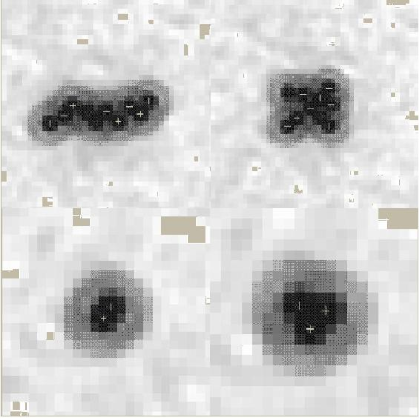
Figure 5: Shown here are four simulated images used for testing of the passive (top row) and active (bottom row) deblending. The sources in the top row are separated by at least one FWHM of the PRF, the 2 sources in the bottom row left picture are separated by $\sim$ 1/2 of the FWHM, and the 3 sources in the bottom row right picture are separated by $\sim$ 2/3 of the FWHM. The locations of the source are shown with white crosses.

We performed simulations to test the limits of passive and active deblending. To test passive deblending a set of point sources with the same flux was added to a smooth background image. The average separation between the adjacent sources was approximately the FWHM (full width half maximum) of the PRF. Two examples of such a cluster with 10 point source is shown in Figure 5. These sources were separated at the detection stage, i.e. they were detected as separate sources. They were marked as belonging to one initial cluster and were fit simultaneously. The simulation was repeated several times for a number of sources ranging from 2 to 20. In Table 1 we show the processing time and the accuracy of determining positions and fluxes. The positional error $\delta_{R}$ is defined as the average distance between the true ${\mathbf{R}}_{n}^{T}$ and extracted ${\mathbf{R}}_{n}^{E}$ positions of the point sources $n$:

$$\delta_{R}=\frac{1}{N_{p}}\sum_{n}^{N_{p}}|{\mathbf{R}}_{n}^{T}-{\mathbf{R}}_{n}^{E}|.$$ (6)

The relative flux error $\delta_{f}$ is defined as the average ratio of the absolute difference between the true $f_{n}^{T}$ and extracted flux $f_{n}^{E}$ to the true flux:

$$\delta_{f}=\frac{1}{N_{p}}\sum_{n}^{N_{p}}\frac{|f_{n}^{T}-f_{n}{E}|}{f_{n}^{T}}.$$ (7)

The processing time was measured on a 1 GHz Sparc Sun workstation with the fitting area of the size of 7 by 7 pixels. The processing time depends on a variety of other factors, so the numbers quoted in Table 1 can be used as a general guide only.

To test active deblending we performed similar simulations. The goal of these simulations was to test the limit in terms of the algorithm’s ability to de-blend sources that cannot be separated at the detection stage. We simulated images with the clusters of 2 and 3 point sources. The distance between the sources in the 2-source clusters was $\sim$ 1/2 of the FWHM, the distance between the sources in the 3-source clusters was $\sim$ 2/3 of the FWHM. In the bottow row of Figure 5 we show an example of a 2-source cluster and a 3-source cluster. The positional and flux errors were $\delta_{R}=0.03$ pixel and $\delta_{f}=0.01$ for the 2-source clusters and $\delta_{R}=0.01$ pixel and $\delta_{f}=0.004$ for the 3-source clusters. The numbers are slightly lower for the 3-source clusters. This is explained by the fact that the separation is greater for these clusters. The important figure of merit is the failure rate $ER$, which is the fraction of the cases for which the algorithm could not succesfully deblend the sources. For the 2-source clusters $ER\sim 0.06$. For the 3-source clusters, even though the separation is greater, the failure rate increases dramatically to $ER\sim 0.25$. Active deblending of clusters with more than 3 sources is not reliable.

An example of passive and active deblending in the real data is given in Figure 2a. The cluster of sources for which both passive and active deblending was performed is circled with the dashed line.

5.2 Output

The output is a list of point sources that specifies their world and local coordinates, fluxes, uncertainties, goodness-of-fit measure, estimated SNR, and a number of other quantities that are used for quality assessment. The flux, position and background uncertanties $\sigma_{z_{i}z_{i}}$ and cross-correlation $\sigma_{z_{i}z_{j}}$ are determined by the diagonal elements of the inverse of the Hessian matrix:

$$H_{z_{i}z_{j}}=\frac{\delta^{2}\chi^{2}}{\delta z_{1}\delta z_{2}};$$ (8)

where $z_{i},z_{j}$ are the fit parameters $f$, $x$, $y$, and $b$.

$$\sigma_{z_{i}z_{j}}=H^{-1}_{z_{i}z_{j}};$$ (9)

SNR for point source with flux $f$ and position ${\mathbf{R}}$ is computed as

$$SNR=\frac{f}{N({\mathbf{R}})NP}$$ (10)

where $N$ is the noise image, described in Section 3; $NP$ is defined as the effective number of pixels whose noise contributes to the measurement of the flux of the point source.

One can specify an unlimited number of apertures to compute aperture photometry for each extracted point source.

5.3 Software

MOPEX consists of a number of modules written in C/C++ which are glued together by perl scripts. Specifically, the point source extraction in the mosaic mode discussed in this paper is performed by the perl script apex_1frame.pl. PRF estimation is performed by the perl script prf_estimate.pl. Point source subtracted images are created with the perl script apex_qa.pl. The software parameters are input through namelists, ASCII configuration files. The software is available for download at the Spitzer website. The documentation included in the distribution has a detailed description of the parameters used in point source extraction as well as sample namelists.

6 PRF Estimation

Here we give a brief description of PRF estimation, which will be described in more details elsewhere. The first time point source extraction can be performed with a theoretical PRF or even a Gaussian PRF. It is performed with a high detection threshold in order to find bright sources. An additional selection should be performed to find only non-confused point sources. A set of postage stamp images is cut out from the background subtracted mosaic image centered on each point source position. More accurate point source positions are estimated by fitting a Gaussian to the postage stamp images. There is an option of rejecting and replacing outlier pixels and outright rejecting ”bad” images. The postage stamp images are resampled and shifted using bicubic interpolation (Meijering et al., 1999) and combined into one final PRF image.

We want to emphasize here that the use of the term PRF is not just an alternative way of saying point spread function (PSF). PSF-fitting is a commonly used term. However, PRF and PSF are two different objects. PSF is an image a point source. PSF is often oversampled, i.e. the pixel size of the PSF image is a fraction of the pixel size of the detector array or the mosaic image for which the PSF is applicable. PRF, however, is not an image of a point source. It is a table of values of responses of the detector array (or mosaic) pixels to a point source. The positions of the pixel for which the response is calculated are on a grid. Normally the PRF is oversampled, which means that the spacing of the grid is a fraction of the detector pixel size. The two - PRF and PSF - are one and the same if they are not oversampled, i.e. the pixel size of the PSF is equal to the pixel size of the detector array(mosaic) and equal to the grid spacing of the PRF. The advantage of using PRF vs. PSF has to do with the way they are derived from the data. PRF is closer to what is being observed by the detector array pixels. Every processing step inevitable introduces errors in the product being calculated. The only error introduced in estimating PRF is the one produced by the shift of the observed pixels to the fixed grid. Estimation of the PSF involves an additional step of interpolating from the bigger detector array pixels to the smaller PSF pixels. This step introduces an additional error. However, for the purposes of fitting one has to reverse this and integrate the small pixels back into the bigger detector array pixels.

7 Application to Spitzer and DSS data

We performed point source extraction on the mosaic images taken at 24 and 70 $\mu$m with MIPS as part of the extragalactic First Look Survey (FLS) (Fadda et al., 2005; Frayer et al., 2005). These images consist of a main shallow survey, centered on a region near the ecliptic pole (RA[J2000]=17:18, Dec[J2000]=+59:30) and covering 4.4 square degrees, and deeper observations (verification strip) contained in the main survey but smaller in size (0.26 square degrees).

7.1 MIPS24 Mosaic

The 24 $\mu$m data was mosaicked to include both the shallow (median coverage of 23) survey and the smaller verification strip (median coverage of 116). The mosaic was created with square pixels measuring half of the detector’s original pixel size, i.e. 1.275 arcsec. The effective integration time for the verification strip is $\sim$426 seconds, about five times deeper than the main field with its $\sim$84 seconds. The noise at 3$\sigma$ is 0.08 mJy (verification strip) and 0.16 mJy (main field).

Point source extraction is performed on the mosaic image, since MIPS24 data is well sampled and usually have a high coverage depth as is the case for the FLS data. Detection and point source fitting is done in a 5 step process. The first step consists of selecting point sources for PRF estimation. As an initial guess a theoretical PRF produced by the Spitzer version of the Tiny Tim Point Spread Function (PSF) modeling program was used. Point source extraction is performed without doing active deblending and only the brightest non-confused (non belonging to a blend of detections) sources (flux $>5\times 10^{3}$ microJy) with the lowest $\chi^{2}$ ($\chi^{2}/dof<30$) are kept. A total of 27 sources are selected for PRF estimation. The second step is to estimate the PRF based on the selected sources. The first Airy ring of the PSF is at a radius of 7 mosaic pixels. We select a PRF postage stamp size of 35 by 35 pixels and a circular PRF with radius of 11 pixels (beyond the first Airy ring). The PRF flux is normalized within that radius and therefore an aperture correction (a factor of 1.156) needs to be applied to all fluxes (Fadda et al., 2005).

The first bright Airy ring around the brightest point sources in our mosaic image are the cause of many false detections in the mosaic image. Therefore, our third step is to create a mosaic image where all the point sources with SNR $>$ 20 in the point source probability image have had their Airy rings removed. This is an example of how the basic processing chain can be modified in order to accomodate specific features of the data. A total of 1224 sources are extracted. Then a residual image is created where the PRF used for subtracting point sources has a hole with a radius of 5 image pixels (where the first minimum occurs in the PRF).

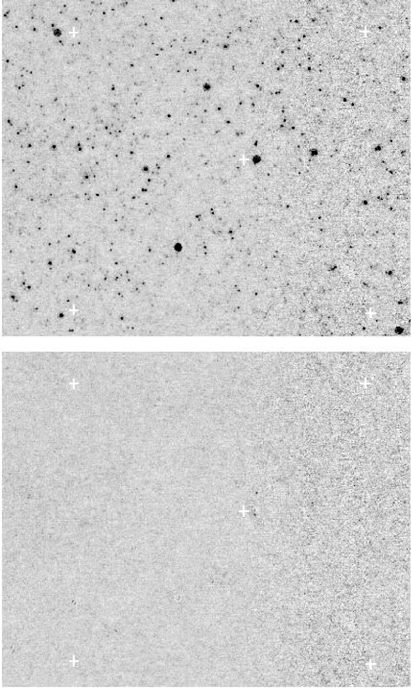
Figure 6: Shown here is a section (1000 by 800 pixels or 0.1 square degree) of the MIPS24 FLS mosaic with the point sources (top) and after point source subtraction (bottom). The section is divided between the verification strip (left part of the mosaic) and the main field outside of the verification strip (right part of the mosaic). Several evenly spread positions are marked with white crosses as reference points in both mosaic images.

The detection is then done on the ringless image with a much lower detection threshold. A total of 97512 sources are detected. The final fitting is done with passive and active deblending. A total of 41559 sources ($\sim 1.0\times 10^{4}$ sources per square degree) with SNR $>$ 3 are extracted. Figure 6 shows a section of the mosaic (1300 by 1000 pixels or 0.16 square degree in size) that has the verification strip and the main field outside of the verification strip. The point source subtracted mosaic is also shown to assess the quality of point source extraction.

7.2 MIPS70 Mosaic

The 70 $\mu$m data was mosaicked to contain only the verification strip (median coverage of 35). The mosaic covers 0.4 square degrees and the pixel size is 4 arcsec. The effective integration time is $\sim 210$ seconds. The total number of extracted point sources with fluxes $>3\sigma$ ($\sim 6$ mJy) is $\sim 400$. The processing steps here are similar to the ones used for the MIPS24 mosaic. The only difference is that we did not create a ”ringless” image for the detection. The reason the Airy rings did not cause any false detection is that even for the brightest sources they are below the noise level. The main reason we use the mosaic mode of point source extraction for MIPS70 data is that in the single frame the data is too noisy to do any dependable point source fitting and PRF estimation.

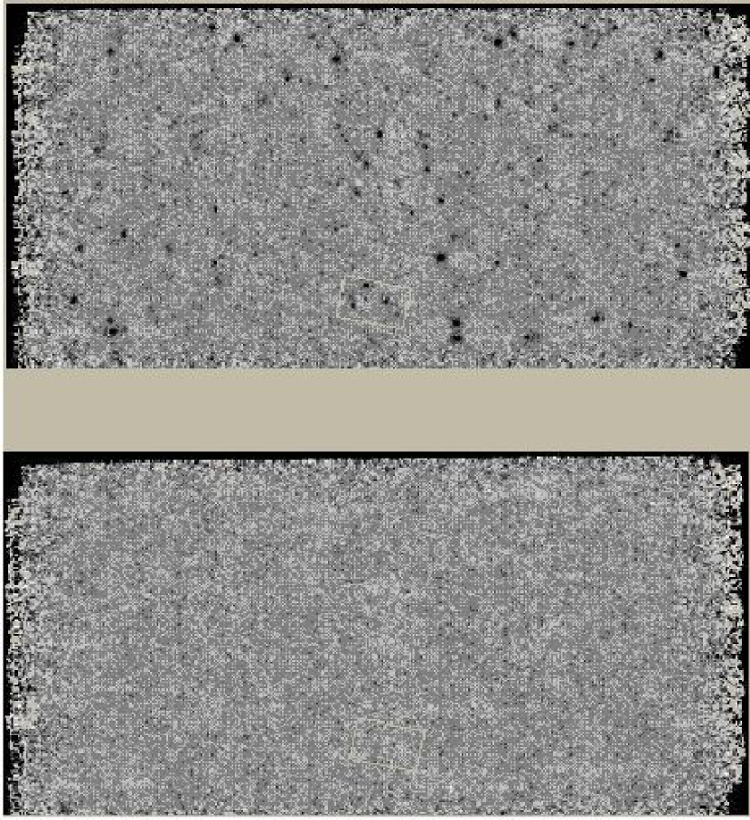
Figure 7: The top image is the MIPS70 mosaic for the verification strip of the FLS. The bottom image is the mosaic with point sources subtracted. The white rectangle shows the fragment of the mosaic used for illustration of processing steps in Figure 2.

Figure 7 shows the MIPS70 mosaic of the verification strip with and without the point sources. The white rectangle shows the fragment of the mosaic used for illustration of the processing steps in Figure 2.

7.3 Digital Sky Survey Image

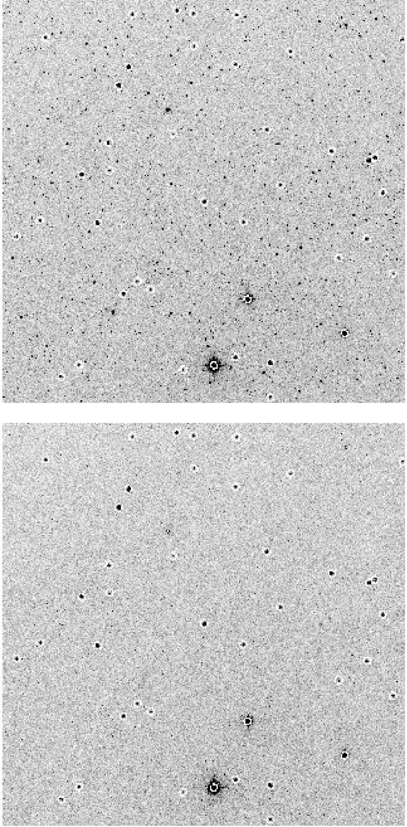
Figure 8: The top image is the DSS image described in the text. The bottom image is the same image with point sources subtracted. The white cirles mark the saturated or extended sources that could not be fit to any satisfaction.

We also tested MOPEX on a Digital Sky Survey (DSS) image, of size 40 arcmin across, near the standard star Landolt 92-288 at position RA[J2000]=00:57:17.093 and Dec[J2000]=+00:36:47.76 (DSS1, plate dss27753). A total of 2836 sources were detected. Figure 8 shows the DSS image and the residual image. Point source extraction was done in two steps. A number of sources in the images have their responses distorted due to non-linear response and several brighter ones are saturated. Also there is a number of extended sources in the field. The separation between good sources, non-linear sources and saturated sources can be done based on the $chi^{2}/dof$ of the fit. At the first step only 2725 good sources were detected and removed from the input image. At the second step 111 non-linear sources were detected and removed from the image. A separate PRF was estimated for the non-linear sources. The quality of the point source extraction and removal for the non-linear sources is obviously worse than for the good sources, but was deemed satisfactory. The fitting and removal for the saturated source cannot be done succesfully. These sources are marked in the Figure 8 with white circles.

8 Validation with Simulated Data

MIPS24 mosaics were simulated by adding point sources to the computed noise images (main and verification). The simulated fluxes were randomly taken from the flux distribution as given by the number counts in the main and verifications surveys (Marleau et al. 2004). A list of true sources was created. The true sources were convolved with the PRF derived previously. Point source extraction done for the real data was repeated with the same steps and parameters on the simulated data.

The list of the true sources used in the simulated images is matched with the list of the extracted sources. Differential completeness and reliability have been measured as function of point source flux density $x$. Completeness $C(x)$ is defined as the ratio of the number of the matched sources $N_{match}(x)$ to the number of the true sources $N_{true}(x)$. Reliability $R(x)$ is defined as the ratio of the number of the matched sources $N_{match}(x)$ to the number of the extracted sources $N_{extract}(x)$:

$$C(x)=\frac{N_{match}(x)}{N_{true}(x)};$$

$$R(x)=\frac{N_{match}(x)}{N_{extract}(x)};$$ (11)

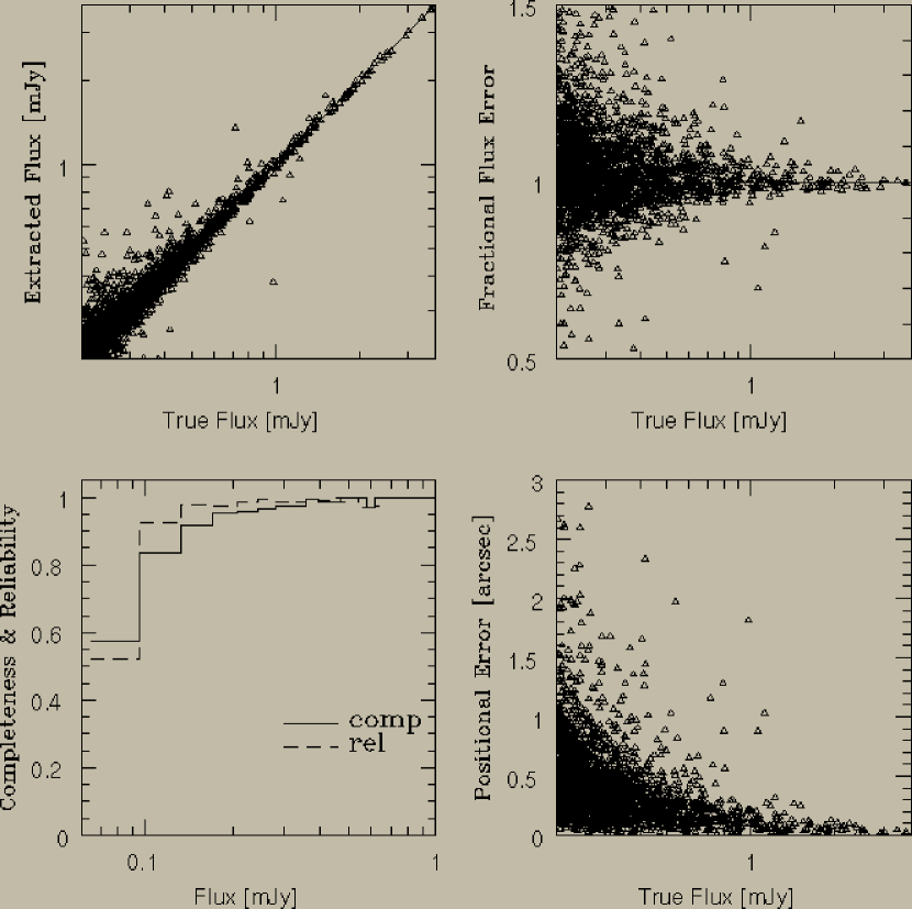
Figure 9: Results of the simulations of the FLS main field for all extracted sources using MOPEX. Top Left: Comparison of the profile fit fluxes from MOPEX with the true fluxes which are used in the simulated FLS main field 24 $\mu$m images. The straight dotted line represents the relation where the MOPEX extracted flux equals the true flux. Top Right: The fractional flux error, the ratio of the extracted flux to the true flux, is plotted as a function of true flux for the matched sources between the extracted and true point source catalogues. Bottom Left: Completeness and reliability measured for the simulated images. Bottom Right: The positional errors as a function of the true flux. The positional errors are calculated by comparing the true and measured positions in the simulated images.

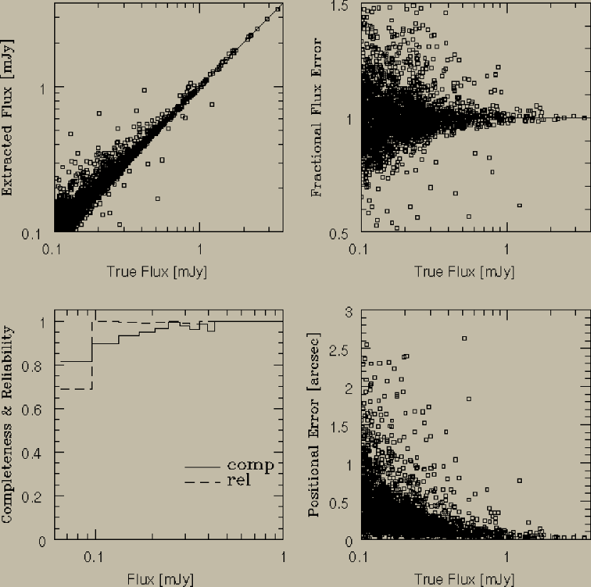
Figure 10: Results of the simulations of the FLS verification strip for all extracted sources using MOPEX. Top Left: Comparison of the profile fit fluxes from MOPEX with the true fluxes which are used in the simulated FLS verification strip 24 $\mu$m images. The straight dotted line represents the relation where the MOPEX extracted flux equals the true flux. Top Right: The fractional flux error, the ratio of the extracted flux to the true flux, is plotted as a function of true flux for the matched sources between the extracted and true point source catalogues. Bottom Left: Completeness and reliability measured for the simulated images. Bottom Right: The positional errors as a function of the true flux. The positional errors are calculated by comparing the true and measured positions in the simulated images.

The results of point source extraction of the simulation data are shown in Figure 9 (main survey) and Figure 10 (verification strip). Comparison of the profile fit fluxes from MOPEX with the true fluxes which are used in the simulated FLS main field 24 $\mu$m images shows a tighter relationship at faint fluxes for the deeper verification strip, as expected. Source extraction is 80% complete at a flux of 0.11 (main) and 0.08 mJy (verification). Within the 80% completeness limit, typical flux measurement errors are of the order of 10-15% (depending on SNR) or less and position accuracy is equal or better than 1 arcsec.

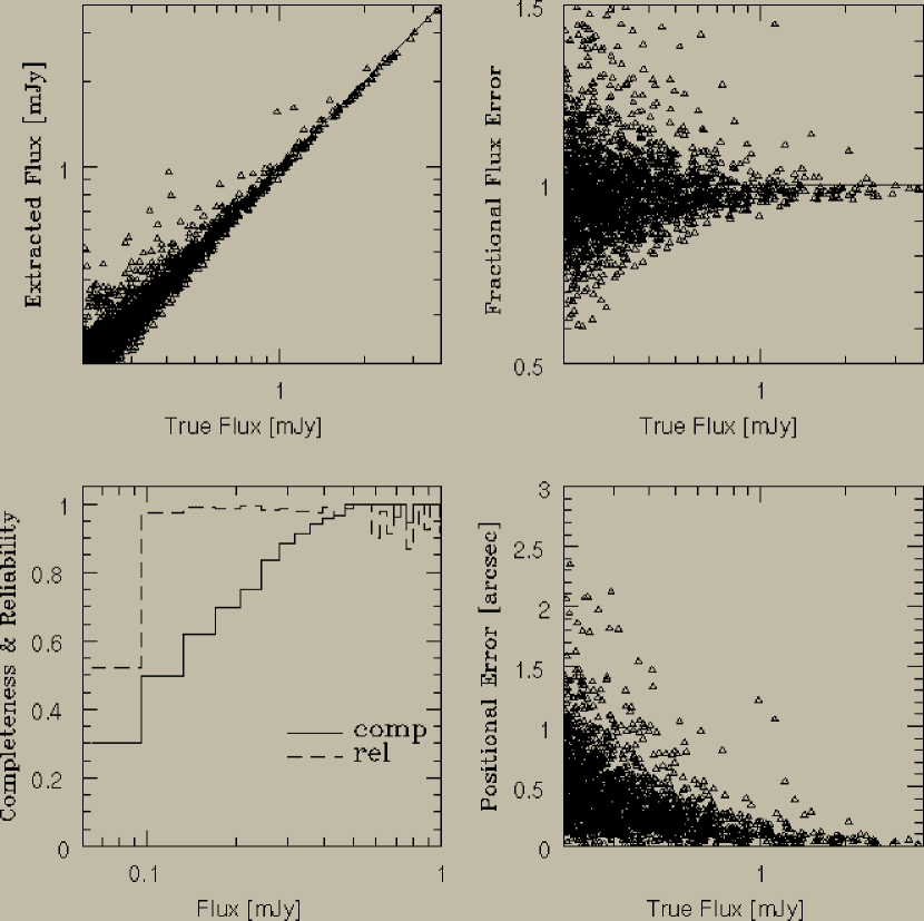
Figure 11: Results of the simulations of the FLS main field for all extracted sources using DAOPHOT.

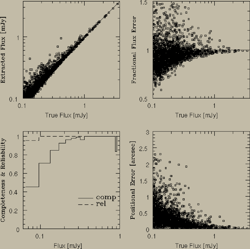
Figure 12: Results of the simulations of the FLS verification strip for all extracted sources using DAOPHOT.

We have performed a simple comparison with another source extraction software, DAOPHOT. DAOPHOT was chosen because it is one of the best known stellar photometry package (Stetson, 1987). It was run as part of IRAF (version 2.12.1). The threshold (in sigma) for feature detection was set to 1.5 and the fluxes were computed within an aperture with radius of 13 pixels. The results of point source extraction of the simulation data with DAOPHOT are shown in Figure 11 (main survey) and Figure 12 (verification strip).

The results produced by MOPEX are arguably better than the ones produced by DAOPHOT. The completeness and reliability of MOPEX extractions are higher overall. That is, the reliability of DAOPHOT extraction is slightly higher, but in our opition the gain in completeness in the much more significant than the loss in reliability. Also MOPEX fluxes have no systematic offsets at the higher end.

8.1 Timing Results

We have performed the timing test for MOPEX on a Solaris machine (SunBlade 2500) with a CPU’s clock rate of 1.5Ghz and 8GB of RAM. We ran MOPEX on the whole 4.4 square degree region and it took only 30 min to complete the point source extraction step (41559 sources extracted with SNR $>$ 3). We also ran DAOPHOT on this image. The DAOPHOT counterpart of point source extraction in MOPEX nstar took 43 min to complete.

9 Conclusion

We presented point source extraction with MOPEX, a package for astronomical image processing developed at the Spitzer Science Center. MOPEX performs point source extraction in two modes: mosaic (single frame) and multiframe. Point source extraction for well sampled data and/or data with high depth of coverage should be done in the mosaic mode. We gave a description of the processing steps of point source extraction in the mosaic mode and the main features that contributed to accurate and efficient extraction. Among them is the non-linear matched filtering leading to improved detection of faint point sources. Passive and active deblending allow for successful fitting of confused point sources. Efficient methods of background and noise estimation and the modified Simplex method contribute to the computational speed of MOPEX.

MOPEX application was shown on the examples of MIPS24 and MIPS70 FLS data and a Digital Sky Survey image. These included the low-level noise MIPS24 verification strip, medium-level noise MIPS24 main field, and high-level noise MIPS70 verification strip. In each case successful point source extraction was evidenced by the quality of the residual images. In order to obtain quantitative evaluation of point source extraction we applied MOPEX to simulated MIPS24 data. We computed the completeness and reliability of point source extraction, as well as the photometric and astrometric accuracy.

For undersampled data with relatively low coverage point source extraction is better done in the multiframe mode by simultaneously fitting sources in the input frames instead of the mosaic image created by coadding the input frames. We will describe the multiframe mode of point source extraction in the near future. Another direction of exploration is applying MOPEX to point source extraction in crowded fields. This will require tuning the algorithm and can potentially lead to some algorithm modification.

Appendix A Non-linear Matched Filter

Here we derive an expression for a non-linear filter based on the notion of point source probability. We assume that image ${\mathbf{s}}$ observed by the detector consists of the point source contribution ${\mathbf{x}}$ convolved with the PRF and additive noise ${\mathbf{n}}$:

$${\mathbf{s}}={\mathbf{H}x}+{\mathbf{n}}.$$ (A1)

Here ${\mathbf{H}}$ is a translationally invariant matrix constructed from the PRF: ${\mathbf{H}_{ij}}={\mathbf{H}_{i-j}}=PRF(i-j)$. The general problem is to estimate the probability of the point source being at a particular pixel i given a measurement vector ${\mathbf{s}}$ in a certain window W surrounding this pixel. The size of the window W is determined by the size of the PRF. We assume that the point source and background noise are characterized by the distribution functions $f_{x}({\mathbf{s}})$ and $f_{n}({\mathbf{s}})$, correspondingly. We consider two hypotheses for the pixel i. The first hypothesis $h_{1}$ is that there is a point source at the pixel, and the second $h_{2}$ (null hypothesis) is that there is not a point source at the pixel. The probability of the $k^{th}$ hypothesis conditioned on the measurement ${\mathbf{s}}$ is given by the Bayesian theorem:

$$P(h_{k}|{\mathbf{s}})=\frac{f({\mathbf{s}}|h_{k})P(h_{k})}{f({\mathbf{s}})},$$ (A2)

where $P(h_{k})$ is the a priori probability of the $k^{th}$ hypothesis, $f({\mathbf{s}})$ is the probability density of observing the set of pixel values ${\mathbf{s}}$. Assuming completeness of the hypothesis set, i.e. $P(h_{1})+P(h_{2})=1$, we obtain for $f({\mathbf{s}})$

$$f({\mathbf{s}})=f({\mathbf{s}}|h_{1})P(h_{1})+f({\mathbf{s}}|h_{2})P(h_{2}).$$ (A3)

The probability density of measurement ${\mathbf{s}}$ under the null hypothesis is given simply by the noise distribution function $f_{n}({\mathbf{s}})$. The probability density of measurement ${\mathbf{s}}$ under the point source hypothesis is the result of integration over all possible point source contributions ${\mathbf{x}}$ :

$$f({\mathbf{s}}|h_{1})=\int d{\mathbf{x}}f({\mathbf{s}}|{\mathbf{x}})f_{x}({\mathbf{x}})=\int d{\mathbf{x}}f_{n}({\mathbf{s}-Hx})f_{x}({\mathbf{x}}).$$ (A4)

Combining everything we obtain for the quantity in question:

$$P(h_{1}|{\mathbf{s}})=(1+\frac{(1-P(h_{1}))f_{n}({\mathbf{s}})}{P(h_{1})\int d{\mathbf{x}}f_{n}({\mathbf{s}-Hx})f_{x}({\mathbf{x}})})^{-1}$$ (A5)

In order to evaluate equation  A5 we assume that both the point sources and the noise have zero-mean Gaussian distribution functions with the variances $\sigma_{x}^{2}$ and $\sigma_{n}^{2}$ and are not correlated spatially. We also assume that there is only one point source in the window W. Under these assumptions the integration in  A4 can be performed to yield:

$$f({\mathbf{s}}|h_{1})=\frac{1}{(\sqrt{2\pi}\sigma_{n})^{W}\sqrt{2\pi}\sigma_{x}}\int dx\exp(-\frac{\sum_{i}(s(i)-PRF(i)x)^{2}}{2\sigma_{n}^{2}}-\frac{x^{2}}{2\sigma^{2}_{x}})=$$

$$\frac{\sigma_{T}}{(\sqrt{2\pi}\sigma_{n})^{W}\sqrt{2\pi}\sigma_{x}}\exp(-\frac{\sum_{i}s^{2}(i)}{2\sigma_{n}^{2}}+\frac{(\sum_{i}s(i)PRF(i))^{2}}{2\sigma_{n}^{4}/\sigma_{T}^{2}}).$$ (A6)

Here

$$\frac{1}{\sigma_{T}^{2}}=\frac{1}{\sigma_{x}^{2}}+\frac{\sum_{i}(PRF(i))^{2}}{\sigma_{n}^{2}}.$$ (A7)

After substituting equation  A in equation  A5 we obtain the final expression for the point source probability:

$$P(h_{1}|{\mathbf{s}})=(1+\frac{(1-P(h_{1}))\sigma_{x}}{P(h_{1})\sigma_{T}}\exp(-\frac{\sum_{i}(s(i)PRF(i))^{2}}{2\sigma_{n}^{4}/\sigma_{T}^{2}}))^{-1}.$$ (A8)

Appendix B Modified Simplex Method

The original downhill simplex algorithm described in Nelder & Mead (1965) and O’Neill (1971) minimizes a function of $N$ variables by using the values of the function at several vertices and trying to move away from the highest vertex. In our paper the function being minimized is the goodness-of-fit measure $\chi^{2}$ defined in equation 4. There are four basic ways to move a vertex: reflection, expansion, contraction and shrinkage.

We adopted the simplex algorithm with a number of improvements. The changes are illustrated in Figure 13. First, we modified reflection. If the change in $\chi^{2}$ is smaller than a user-specified threshold, it is an indication that the reflection is done almost parallel to the iso-$\chi^{2}$ lines. In this case an attempt is made to replace the reflection with a move in a perpendicular direction. The number of perpendicular directions are equal to $2(N-1)$. The move is performed, if it results in a $\chi^{2}$ lower than the one achieved by the reflection.

Another modification is that contraction and shrinkage have been replaced with the line minimization of $\chi^{2}$ along the unsuccessful reflection direction. I.e. if the reflection results in point with higher than the original $\chi^{2}$, a point with the lowest $\chi^{2}$ is found on the line of the unsuccessful reflection.

Without the modifications the algorithm in its original form very often was unable to find the global minimum and remained stuck in of the local minima and wandered away from the true point source location.

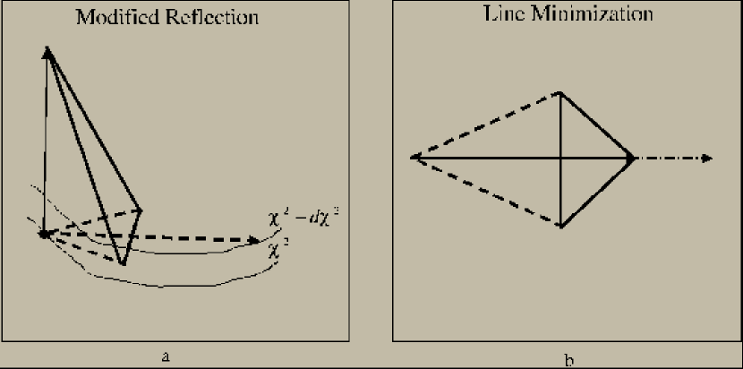
Figure 13: Modifications of the Simplex method. a) The dotted lines are lines of constant $\chi^{2}$. The old simplex is shown with dashed lines. The dashed arrow shows the reflection of the highest vertex based on the old simplex. If the change $d\chi^{2}$ is less than a user specified limit then the vertex is moved as indicated by the solid arrow in a direction perpendicular to the original reflection. b) The original simplex is shown with the dashed lines. If reflection, shown here with the dashed arrow, results in a point with a higher $\chi^{2}$, a point with the lowest $\chi^{2}$ is found along the line of reflection.

Table 1: Test of passive deblending. The average execution time $t_{ex}$, positional $\delta_{R}$ and flux $\delta_{f}$ errors are shown as a function of the number of sources in a cluster $N_{p}$.

$N_{p}$	2	4	6	8	10	12	14	16	18	20
$t_{ex}$(sec)	0.07	0.15	0.43	0.90	1.8	3.3	5.5	9.3	15	20
$\delta_{R}$(10-2pixels)	0.3	0.5	0.8	1.7	2.4	2.6	2.9	3.5	4.3	5.1
$\delta_{f}$(10-2)	0.5	0.8	1.1	1.6	1.9	2.2	2.4	2.7	2.9	3.3

References

- Andrews (1970) Andrews, H.C. Computer Techniques in Image Processing, Academic Press, New York, 1970
- Bertin & Arnouts (1996) Bertin, E. & Arnouts, S. 1996, Astronomy and Astrophysics, Suppl. Ser., 117, 393
- Cook & Bernfeld (1970) Cook, C.E. and Bernfeld M., Radar Signals, Academic Press, New York, 1965
- Diolaiti et al. (2000) Diolaiti, E., Bendinelli, O., Bonaccini, D., Close, L., Currie, D., & Parmeggiani, G. 2000, Astronomy and Astrophysics, Suppl. Ser., 147, 335
- Fadda et al. (2005) Fadda, D. et al. 2005, in preparation
- Frayer et al. (2005) Frayer, D. et al. 2005, in preparation
- Juhola et al. (1991) Juhola, M, Katajainen, J, & Raita, T. 1991, IEEE Transactions on Signal Processing, 39, 204
- Makovoz & Khan (2004) Makovoz, D. and Khan, I. Astronomical Data Analysis Software and Systems VI, 132, in ASP Conf. Ser., San Francisco
- Makovoz (2005) Makovoz, D. 2005, in Proc. of SPIE, 5672, eds. Edward R. Dougherty, Jaakko T. Astola, Karen O. Egiazarian, 358
- Marleau et al. (2004) Marleau, F.R. et al. 2004, ApJS, 154, 66
- Meijering et al. (1999) Meijering E.H.W., Zuiderveld K.J., & Viergever M.A. 1999, IEEE Transactions on Image Processing, 8, 192
- Nelder & Mead (1965) Nelder, J.A., Mead, 1965, R. Comp. J., 7, 308
- O’Neill (1971) O’Neill, R. 1971, Applied Statistics, 20, 338
- Schechter et al. (1993) Schechter, P.L., Mateo, M., Saha, A. 1993, PASP, 105, 1342
- Stetson (1987) Stetson, P.B. 1987, PASP 99, 191