Terrestrial Planet Formation in Disks with Varying Surface Density Profiles
Abstract
The “minimum-mass solar nebula” (MMSN) model estimates the surface density distribution of the protoplanetary disk by assuming the planets to have formed in situ. However, significant radial migration of the giant planets likely occurred in the Solar system, implying a distortion in the values derived by the MMSN method. The true density profiles of protoplanetary disks is therefore uncertain. Here we present results of simulations of late-stage terrestrial accretion, each starting from a disk of planetary embryos. We assume a power-law surface density profile that varies with heliocentric distance as , and vary between 1/2 and 5/2 ( for the MMSN model). We find that for steeper profiles (higher values of ), the terrestrial planets (i) are more numerous, (ii) form more quickly, (iii) form closer to the star, (iv) are more massive, (v) have higher iron contents, and (vi) have lower water contents. However, the possibility of forming potentially habitable planets does not appear to vary strongly with .
Subject headings:
astrobiology — planets and satellites: formation — methods: n-body simulations-0.5in
1. Introduction
In calculating the range of possible terrestrial planet systems that could form around Sun-like stars, it is important to consider protoplanetary disks with surface density profiles different that the standard, “minimum mass solar nebula” model (MMSN – e.g., Weidenschilling 1977). Different disk profiles form protoplanets with different masses and spacings (Kokubo & Ida 2002). The accretion of terrestrial planets from these protoplanets is strongly affected by the distribution of mass in the system, and the dynamical timescales associated with regions of enhanced density. The terrestrial planets that form in disks with varying density profiles may vary in significant ways, e.g. in their compositions and formation timescales. In this paper, we use a standard prescription for disk mass densities, constrained by observations of such disks, to explore how disk properties affect the growth of terrestrial planet systems.
The MMSN model calculates the density profile of the protoplanetary disk in the following way. The mass in each planet is augmented to Solar composition by adding the appropriate amount of light elements. Next, this mass is smeared out into contiguous annuli. Finally, a simple, power-law profile is fit to the corresponding data points. The resulting surface density profile scales with heliocentric distance (in AU) as . Values for range from 1700 (Hayashi 1981) to 4200 (Weidenschilling 1977). In this case, includes both the gas and dust component of the disk. The solid component of the MMSN follows the same profile with .
There is no reason to expect that all disks should follow the standard, MMSN profile. There is evidence that at least the outer planets in our Solar System may have undergone significant radial migration (e.g. Levison & Morbidelli 2003), which would distort the inferred density profile. In addition, certain disk collapse models predict shallower, profiles (Shakura & Sunyaev 1973). In contrast, Kuchner (2004) showed that the mean, minimum-mass extra solar nebula has a steeper, roughly profile. Of course, this steeper profile also assumes that the known extra-solar giant planets formed and remained in situ. In light of studies of planet migration (e.g. Lin et al. 1996), this is not thought to be the case. There is clearly reason to consider protoplanetary disks with surface density profiles different that the MMSN model.
Wetherill (1996) formed planets in both and profiles, and saw no differences between the two cases. Chambers & Cassen (2002) simulated the late-stage accretion of terrestrial planets in two different surface density profiles. One of these was a simple, profile, while the other had a low density in the inner disk, with a peak at roughly 2 AU, based on a temperature dependent condensation model of Cassen (2001). They found that the power law profile generally provided a better fit to the Solar system than the peaked profile, in terms of the number and masses of terrestrial planets formed. There remains a great deal of uncertainty in disk models in terms of redistribution of solids throughout the accretion process, including gas drag, type I migration, and dynamical scattering.
Raymond, Quinn & Lunine (2004; hereafter RQL04) slightly varied the value of , but only between 8-10 . They did, however, vary the surface density in the outer protoplanetary disk by changing the planetesimal mass used in the outer terrestrial zone. We found that a higher surface density results in the formation of a smaller number of less massive planets. These planets also tend to have higher orbital eccentricities. Raymond, Quinn & Lunine (2005; hereafter RQL05) ran two simulations with . The systems that formed resembled extended asteroid belts, containing several Mars-sized bodies but no large terrestrial planets.
We adopt a general power-law distribution (note that bears no relation to the viscosity parameter by the same name). We consider three different power-law surface density distributions, with = 0.5, 1.5 and 2.5. These cases encompass the likely range of actual values, according to theory and observation. We determine the effects of on the accretion process as well as the physical properties of the planets which form, including their mass, composition, and potential habitability.
2. Initial Conditions
We consider three surface density distributions. Each contains 10 Earth masses () of material between 0.5 and 5 AU. Because of their different shapes, each has a different value for . For = 0.5, , for = 1.5, , and for = 2.5, . The mass contained in the inner disk is much higher for higher values of . The disk with has 6.5 of material inside 1.5 AU, compared with 3.6 for and only 1.4 for .
We assume in our initial conditions that oligarchic growth has taken place, and the disk mass is dominated by planetary embryos, shown to be the case for different values of by Kokubo & Ida (2002). Each planetary embryo has swept up the mass in its feeding zone, which has a width of mutual Hill radii. With our generalized power-law density profile, the mass of a given planetary embryo scales with its semimajor axis and the separation between embryos as
| (1) |
For a density profile steeper than = 2, the mass of planetary embryos decreases with heliocentric distance, and the mass is very concentrated close to the star. Conversely, shallower density profiles result in higher-mass planetary embryos at large distances, with more mass in the outer disk. Figure 1 shows the distribution of evenly spaced planetary embryos for each of our surface density distributions. For , embryos are very small in the inner disk and quite massive (up to ) and well-spaced in the outer disk. Conversely, for , embryos are smaller in the outer disk, though better-separated, as the Hill radius has a stronger dependence on semimajor axis than on mass ().
In Fig. 1, is fixed at 7 Hill radii, to demonstrate the differences in embryo mass and spacing. However, in our simulations we space embryos randomly by 1-2 Hill radii from 0.5 to 5 AU. The number of embryos varies for each value of : we include roughly 380 embryos for , 290 embryos for , and 280 embryos for . For each value of , we perform three simulations with different random number seeds.
The starting water contents of embryos are as described in RQL04: embryos are dry inside 2 AU, contain 0.1% water between 2-2.5 AU, and 5% water past 2.5 AU. Their initial iron contents are interpolated between the values for the Solar System planets and chondritic meteorites associated with known classes of primitive asteroids (values from Lodders & Fegley, Jr. 1999). Embryos are given small initial eccentricities () and inclinations ().
In each case we include a Jupiter-mass giant planet at 5.5 AU on a circular orbit. One could argue that if the mass of a giant planet scales with the isolation mass for a given surface density, then the masses of the giant planets should vary in position and mass according to our values of (Lissauer 1995). However, we do not know which profile to be the most common in nature, or whether there even exists a universal density profile for protoplanetary disks. We are constrained by observations of actual extra-solar planets which do form, whatever their initial disk profile. Due to the large amount of uncertainty in this issue, it seems reasonable to assign the same outer giant planet to each disk.
Each simulation was integrated for 200 Myr using the hybrid algorithm of the Mercury integrator (Chambers 1999), with a 6 day timestep. Collisions are treated as inelastic mergers which conserve linear momentum, mass, water and iron content. Each simulation took 1-3 months to run on a desktop PC, and conserved energy to at least one part in .
3. Results
3.1. Details of two Simulations
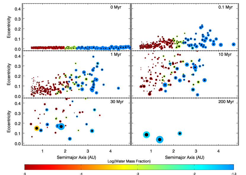
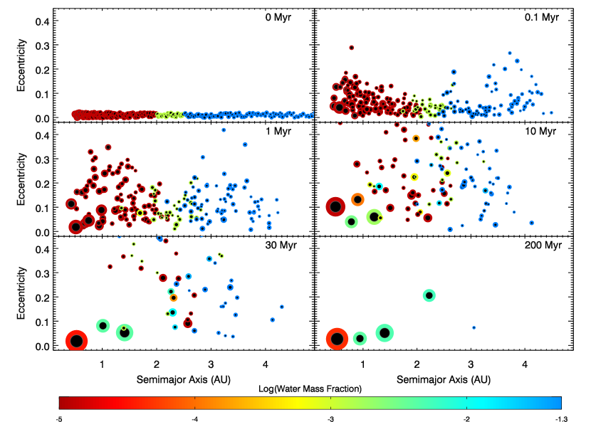
Figures 2 and 3 show the time evolution of two simulations with = 0.5 and 2.5, respectively. The overall progression of both simulations is similar, but the details are quite different. In both cases, the eccentricities of planetary embryos increase until their orbits cross and collisions may occur. This eccentricity pumping occurs due to secular and resonant perturbations from both other embryos and the giant planet at 5.5 AU (which, for simplicity, we now refer to as Jupiter). Many embryos are ejected after close encounters with Jupiter. Larger bodies grow by accreting smaller ones, on timescales which depend on both the dynamical timescale (orbital distance) and the local density of material. Many bodies which form inside 2 AU contain one or more water-rich embryos which began the simulation past 2-2.5 AU. In time, most small bodies are removed from the simulation, either via collisions with the forming planets, the Sun, or Jupiter, or via ejection from the system. What remains are a few (typically 2-4) terrestrial planets with significant masses, generally inside 2 AU. The details of the planets which have formed in Figs. 2 and 3 are summarized in the captions.
The main difference between the two simulations has to do with their different mass distributions, and can be easily seen in a comparison of the eccentricities of the inner disk in the 0.1 Myr panels of Figs. 2 and 3. In 2, where = 0.5, the majority of the terrestrial mass is in the outer disk, past 2.5 AU. Eccentricity pumping occurs mainly in the outer disk, via both mutual encounters and interactions with Jupiter, and the terrestrial planets therefore form from the outside in. The planets which form contain a large amount of water-rich material, simply because so much initial material was found in the outer disk. The final planets contain only a small fraction of the initial mass, because embryos in the outer disk are very strongly excited by Jupiter, and largely ejected from the system.
In Fig. 3, where = 2.5, the majority of the mass lies inside 2.5 AU. The eccentricities of embryos in the inner disk are self-excited through mutual gravitational interactions. Accretion proceeds quickly in the inner regions due to both the high density of material and short dynamical timescales. Terrestrial planets therefore form from the inside out. Most of the mass in the system is well-separated from Jupiter, so the final planets contain the majority of the initial mass. However, since there was little initial water-rich mass past 2.5 AU, they are much drier than in Fig. 2.
3.2. Trends with
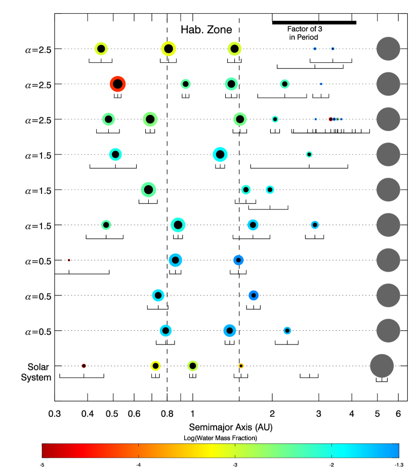
Figure 4 shows the final configuration of all nine simulations we performed, with the Solar System shown for comparison. Our simulations with = 1.5 do not reproduce the Solar System planets as well as previous simulations with the same profile, such as RQL04. This is because the total mass in the disk is higher in these simulations. The 10 in the terrestrial region is roughly twice as much as in the MMSN model, and 50% higher than in RQL04 (higher still for the case (ii) simulations). As shown in RQL04, a higher surface density of material results in the formation of a larger number of more massive planets with larger eccentricities. We see the results of this effect in comparing the = 1.5 simulations with the Solar System in Fig. 4. None of our simulations form Mars-sized planets inside 2 AU, also because of the large total mass in protoplanets. Although this affects certain comparisons between our results and the Solar System planets, it does not affect comparisons between simulations with similar initial conditions.
There exist several strong correlations between the final planetary systems and the slope of the density profile, , which are shown in Table 1. Perhaps the most striking is simply the location of the planets formed. In cases with = 1.5 and 2.5, the innermost planet typically resides around 0.5 AU, while the innermost planet in the = 0.5 simulations is usually around 0.75 AU. It is important to note that in this analysis we define a planet to be a body larger than 0.2 whose orbit lies inside 2 AU.
| Trend | |||
|---|---|---|---|
| Mean innermost planet11We define a planets to be more massive than 0.2 Earth masses and to have semimajor axis 2 AU. | 0.74 AU | 0.47 AU | 0.45 AU |
| Mean planet mass | 1.4 | 1.7 | 2.2 |
| Mean formation time22Mean time to reach 90% of a planet’s final mass. See Fig. 5. | 55 Myr | 42 Myr | 18 Myr |
| Mass (planets) / Mass (disk)33Fraction of initial disk mass contained in final planets | 0.28 | 0.44 | 0.65 |
| Total mass in planets | 2.8 | 4.4 | 6.5 |
| Mean number of planets | 2.0 | 2.67 | 3.0 |
| Mean number of planets 1 AU | 1.0 | 1.3 | 2.0 |
| Avg. mass of planets 1 AU | 1.65 | 2.06 | 2.24 |
| Mean largest planet | 1.75 | 2.8 | 3.0 |
| Mean orbital eccentricity | 0.07 | 0.12 | 0.06 |
| Mean water mass fraction | |||
| Mean iron mass fraction | 0.19 | 0.27 | 0.29 |
| Avg. num. of habitable planets44Habitable planets are defined to have semimajor axes between 0.8 and 1.5 AU, and water mass fractions larger than . | 1.0 | 2/3 | 2/3 |
The trends from Table 1 can be summarized as follows. As compared with a protoplanetary disk with a shallow surface density profile, a disk with a steeper surface density profile forms a larger number of more massive terrestrial planets in a shorter time. Figure 5 shows the mean time for planets to reach 50%, 75%, and 90% of their final mass for all three values of . The reason that = 0.5 planets form more slowly is that the timescale for accretion scales with the dynamical time and the local density. The density in the outer disk is high enough that planets form more from the outside in. The long dynamical timescales translate to slower planet growth, and planets at larger heliocentric distances. In the case of = 2.5 planets, the high inner density and fast dynamical timescales conspire to form planets on remarkably short timescales. There is a constraint from measured Hf-W ratios that both the Moon and the Earth’s core were formed by 30 Myr (Kleine et al. , 2002; Yin et al. , 2002), suggesting that the Earth was at least 50% of its final mass by that time. Fig. 5 shows that planets in each of our density profiles satisfy this constraint.
A larger number of planets is formed in the simulations with = 2.5 because the planets in those simulations occupy a larger range in semimajor axes, i.e. they extend to smaller orbital radii than for = 0.5. The mean orbital radii of the innermost planet for = 2.5 and = 0.5 simulations are 0.45 AU and 0.74 AU, respectively. This corresponds to a difference in orbital period of over a factor of two, providing enough dynamical room for another planet. Indeed, the = 2.5 simulations formed an average of three planets per simulation, as compared with two planets per simulation for = 0.5.
The reason that more mass ends up in planets for steeper density profiles is the dynamical presence of Jupiter. During accretion, a large fraction of the material close to Jupiter is ejected from the planetary system. The “ejection range” of Jupiter, the zone from which a large fraction of material is ejected, extends to a factor of 4-6 in orbital period (a factor of 2.5-3.3 in semimajor axis) from Jupiter. If we naïvely assume as in RQL05 that all material within a factor in orbital period of Jupiter is ejected from the system, then the total mass ejected is
| (2) |
where is the orbital radius of Jupiter. The value of depends on the mass and eccentricity of the giant planet, and may also scale with and . If we only consider material ejected from interior to the giant planet, then
| (3) |
We know the values of and the mean amount of mass ejected per simulation for each value of , so we can calculate a value for (we also take into account the fact that embryos exist only out to 5 AU, while = 5.5 AU). We find that ranges between roughly 4 () and 6 (). The mean location of the outermost planet in each simulation, independent of , was at about the 5:1 resonance with Jupiter (at 1.9 AU), consistent with our values of . The range at which Jupiter ejects material from an = 2.5 disk appears to be farther than for an = 0.5 disk (Jupiter’s effective “ejection range” is the 6:1 vs 4:1 resonance for = 2.5 and 0.5, respectively). The reason for this increased range for = 2.5 is the lack of material in the outer disk with which excited embryos may interact, possibly damp their eccentricities, and remain in the disk. A particle excited by Jupiter in an = 0.5 disk may have its eccentricity subsequently decreased via embryo-embryo interactions, whereas the dearth of material in the outer disk prevents this from happening for = 2.5.
We perform a MMSN-like test on the planets which formed. For each system, we select all planets of 0.2 or more and spread their mass into concentric, nested annuli, and calculate an effective surface density. We choose the division of annuli between two planets to be the geometric mean of the semimajor axes of the two planets, following Kuchner (2004). For , we find a best-fit slope to the surface density, , of almost exactly 2.5. However, we obtain values between 2.1 and 2.3 for the planets formed in = 0.5 or 1.5 simulations. The reason for this is because, as discussed above, Jupiter’s ejection of material from the asteroid region has a much stronger effect on shallower density profiles. This decreases the surface density measurements for outer radii, skewing the fit to a steeper profile. If we only include planets inside 2 AU, outside of Jupiter’s ejection range, the for the = 1.5 planets changes to 1.53. However, for the = 0.5 planets remains above 2, because of Jupiter’s pervasive effects in low- simulations. Choosing an even smaller outer radius would likely yield a value closer to 0.5, but the number of planets is too small to perform the test. This analysis implies that, in the absence of external perturbations (e.g. from the giant planets), terrestrial accretion forms planets that conform to their initial density profile. In this sense, the planets “remember” the initial state of the disk.
This begs the question of why the Solar system planets follow an profile. Two explanations are possible: 1) the surface density profile of the protoplanetary disk followed an profile, or 2) the initial profile was different, but perturbations caused the final planets to follow an altered profile. If perturbations did affect the final planets, then the starting mass profile was likely flatter, i.e., the starting value of was smaller than 1.5. However, as demonstrated above, the ejection range of Jupiter extends inward to orbital radii of 2 AU. Additional secular perturbations arise from the presence of Saturn (e.g. the secular resonance at 2.1 AU). But the inner terrestrial region remains relatively sheltered from these perturbations. In addition, the giant planets’ eccentricities may have been significantly lower during the epoch of terrestrial accretion (Tsiganis et al. 2005), reducing the effect of secular resonances. We conclude that the inner solar nebula probably did follow an profile.
The probability of a habitable planet forming between 0.8-1.5 AU with water mass fraction does not depend strongly on the value of , although planets that form in disks with different values will certainly have vastly different characteristics. Planets that form with = 2.5 have much higher iron contents than those in = 0.5 disks, simply because the amount of iron-rich material close to the star is much higher. Similarly, planets that form in = 0.5 disks have much higher water contents than those in = 1.5 or 2.5 disks, because the bulk of the solid mass in = 0.5 disks is found in the water-rich outer regions. The iron and water contents will have large consequences for the nature of the surface and interior of these planets, as well as their potential habitability.
4. Discussion
The true surface density profiles of the solid component of protoplanetary disks are unclear. Their formation involves a great deal of physics, including the condensation sequence as a function of temperature, and radial migration via gas drag and type I migration. It is likely that the standard, minimum mass solar nebula model is oversimplified, as there is strong evidence from the dynamical structure of the Kuiper belt that the giant planets experienced significant radial migration (Levison & Morbidelli 2003).
We have demonstrated that the terrestrial planets which form in protoplanetary disks with three different power-law surface density profiles have very different characteristics. The total number and mass of terrestrial planets is strongly affected by the surface density slope, . In the presence of an outer giant planet, a disk with a steeper profile (higher ) yields a larger number of more massive planets than a shallower profile. Planets in steeper-profiled disks form more quickly, have higher iron content and lower water content than for shallower profiles, with implications for the habitability of planets in each case.
It is unclear whether our placement of a Jupiter-mass giant planet at 5.5 AU is self-consistent for each chosen value of . Kokubo & Ida (2002) and Lissauer (1995) argued that the character of the giant planets may depend on the disk’s density profile. We chose identical initial conditions to explore the effects of in a “typical” planetary system, although the nature of such a system may be inextricably linked to . Some of our results that were strongly influenced by the presence of a giant planet, such as the strong depletion of the disk, may only hold under our given assumption of a giant planet at 5.5 AU. However, many of our results are independent of this assumption, such as the formation timescales and compositions of the planets we form.
Using previous results, we can extrapolate the effects of other parameters on our simulations, such as giant planet orbital radius and eccentricity, and the location of the snow line. It has been shown that a giant planet on an eccentric orbit forms terrestrial planets which are drier, less massive, and have larger eccentricities than for a giant planet on a circular orbit (Chambers & Cassen, 2002; RQL04). In the presence of an eccentric giant planet, more of the material from the asteroid region is ejected, and planets form at a larger distance from the giant. Therefore, an eccentric giant planet would cause even more disparity between disks with shallow vs. steep density profiles. A disk with would have an even higher fraction of its total mass ejected, causing the terrestrial planets to be smaller. An disk, however, would not be strongly affected, since its mass is so centrally concentrated. The primary consequence of the giant planets’ orbital radius is the amount of solid material destroyed through ejection from the system. This will vary with heliocentric distance and as shown in equation 2. The location of the snow line determines how much water-rich material exists in disks with different values of .
Kuchner (2004) found that applying the MMSN technique to the known, extra-solar planets yielded a very steep density profile with . This steep profile corresponds to an in situ formation scenario for close-in giant planets (e.g. “hot jupiters”). If such a profile is common, then perhaps hot jupiters exist in these systems. We expect that terrestrial planets may form in the presence of a hot jupiter, even if it has migrated through the terrestrial region (RQL05). Indeed, terrestrial planets appear to be able to form in some of the known extra solar planetary systems, such as 55 Cancri (Raymond & Barnes 2005).
Real protoplanetary disks are not perfectly smooth power laws. The physics and chemistry determining their true shape is very complex, and has not been fully modeled. Some preliminary models show a peak in surface density around 1-2 AU (Cassen 2001), which may explain the large masses of Venus and Earth (Chambers & Cassen 2002). Such a profile can be roughly approximated as having a small value in the inner disk, and a larger value past 2 AU. We have shown that accretion proceeds from the inner disk outwards for large and from the outer disk inwards for smaller values. In this composite disk, accretion would likely start in the highest density region around 1-2 AU, and proceed both inward and outward.
5. Acknowledgments
We thank referee John Chambers for bringing up some important points. This work was funded by grants from NASA Astrobiology Institute and NASA Planetary Atmospheres. These simulations were run under Condor111Condor is publicly available at http://www.cs.wisc.edu/condor.
References
- (1) Cassen, Patrick 2001. Nebular thermal evolution and the properties of primitive planetary materials. Meteoritics and Planetary Science, 36, 671
- (2) Chambers, J. E., 1999. A Hybrid Symplectic Integrator that Permits Close Encounters between Massive Bodies. MNRAS, 304, 793-799.
- (3) Chambers, J. E. & Cassen, P., 2002. The effects of nebula surface density profile and giant-planet eccentricities on planetary accretion in the inner solar system. Meteoritics and Planetary Science, 37, 1523-1540.
- (4) Hayashi, C. 1981. Structure of the solar nebula, growth and decay of magnetic fields and effects of magnetic and turbulent viscosities on the nebula. Prog. Theor. Phys. Suppl., 70, 35-53.
- (5) Kasting, J. F., Whitmire, D. P., and Reynolds, R. T., 1993. Habitable zones around main sequence stars. Icarus 101, 108-128.
- (6) Kleine, T., Munker, C., Mezger, K., Palme, H., 2002. Rapid accretion and early core formation on asteroids and the terrestrial planets from Hf-W chronometry. Nature 418, 952-955.
- (7) Kokubo, E. & Ida, S., 2002. Formation of Protoplanet Systems and Diversity of Planetary Systems. ApJ 581, 666.
- (8) Kuchner, M. J. 2004. A Minimum Mass Extrasolar Nebula. ApJ, 612, 1147
- (9) Levison, H. F. & Morbidelli, A. 2003. The formation of the Kuiper belt by the outward transport of bodies during Neptune’s migration. Nature, 426, 419
- (10) Lin, D. N. C., Bodenheimer, P., & Richardson, D. C., 1996. Orbital migration of the planetary companion of 51 Pegasi to its present location. Nature, 380, 606-607.
- (11) Lissauer, J. J. 1995. Urey Prize Lecture: On the Diversity of Plausible Planetary Systems. Icarus 114, 217-236.
- (12) Lodders, K., & Fegley, B. 1998, The planetary scientist’s companion. Oxford University Press, 1998.
- (13) Raymond, S. N., Quinn, T., & Lunine, J. I., 2004. (RQL04) Making other earths: dynamical simulations of terrestrial planet formation and water delivery. Icarus, 168, 1-17.
- (14) Raymond, S. N., Quinn, T., & Lunine, J. I. 2005. (RQL05) The formation and habitability of terrestrial planets in the presence of close-in giant planets. Icarus, in press.
- (15) Raymond, S. N. & Barnes, R. 2005. Predicting Planets in Known Extra-Solar Planetary Systems III: Forming Terrestrial Planets. ApJ, submitted, astro-ph/0404212
- (16) Shakura, N. I., & Sunyaev, R. A. 1973. Black holes in binary systems. Observational appearance. A&A, 24, 337
- (17) Tsiganis, K., Gomes, R., Morbidelli, A., & Levison, H. F. 2005. Origin of the orbital architecture of the giant planets of the Solar System. Nature, 435, 459
- (18) Weidenschilling, S. J. 1977. The distribution of mass in the planetary system and solar nebula. Ap&SS, 51, 153
- (19) Wetherill, G. W., 1996. The Formation and Habitability of Extra-Solar Planets. Icarus, 119, 219-238.
- (20) Yin, Qingzhu, Jacobsen, S. B., Yamashita, K., Blichert-Toft, J., Telouk, P., Albarede, F., 2002. A short timescale for terrestrial planet formation from Hf-W chronometry of meteorites. Nature 418, 949-952.