STEllar Content and Kinematics from high resolution galactic spectra via Maximum A Posteriori

Abstract

We introduce STECKMAP (STEllar Content and Kinematics via Maximum A Posteriori), a method to recover the kinematical properties of a galaxy simultaneously with its stellar content from integrated light spectra. It is an extension of STECMAP (Ocvirk et al., 2005) to the general case where the velocity distribution of the underlying stars is also unknown. The reconstructions of the stellar age distribution, the age-metallicity relation, and the Line-Of-Sight Velocity Distribution (LOSVD) are all non-parametric, i.e. no specific shape is assumed. The only a propri we use are positivity and the requirement that the solution is smooth enough. The smoothness parameter can be set by generalized cross validation according to the level of noise in the data in order to avoid overinterpretation.

We use single stellar populations (SSP) from Pégase-HR ($R=10\,000$, $\lambda\lambda=4\,000-6\,800$ Å, Le Borgne et al. 2004) to test the method through realistic simulations. Non-Gaussianities in LOSVDs are reliably recovered with SNR as low as $20$ per $0.2$ Å pixel. It turns out that the recovery of the stellar content is not degraded by the simultaneous recovery of the kinematic distribution, so that the resolution in age and error estimates given in Ocvirk et al. (2005) remain appropriate when used with STECKMAP.

We also explore the case of age-dependent kinematics (i.e. when each stellar component has its own LOSVD). We separate the bulge and disk components of an idealized simplified spiral galaxy in integrated light from high quality pseudo data (SNR=100 per pixel, R=$10\,000$), and constrain the kinematics (mean projected velocity, projected velocity dispersion) and age of both components.

1 Introduction

For decades now, the spectral indices from the Lick group have been used to study the properties of stellar populations (Faber et al., 1985; Worthey, 1994; Trager et al., 1998). Since the profile and depth of the lines involved in these spectral indices are affected by the Line Of Sight Velocity Distribution (hereafter LOSVD) of the stars, it is necessary to correct the measured depths by a factor depending on the moments of the velocity distribution (Davies et al., 1993; Kuntschner, 2000, 2004). The latter moments must be determined using specialized code (Bender, 1990; Saha & Williams, 1994; Pinkney et al., 2003; Merritt, 1997; Kuijken & Merrifield, 1993; van der Marel & Franx, 1993). These kinematical deconvolution routines have been used for some time and have undergone 2 major mutations. First, thanks to the increasing power of computers, it became affordable to swap back and forth from direct space to Fourier space, so that many disturbances such as border effects and saturation could be avoided. It became straightforward to mask problematic regions of the data, such as dead pixels, emission lines, etc… The second evolution of these codes allowed the use of multiple superimposed stellar templates to best match the observed spectrum (Rix & White, 1992; Cappellari & Emsellem, 2004). It has also been proposed to use single stellar populations as synthetic templates, and this approach has proved to be useful in addressing the template mismatch problem (Falcón-Barroso et al., 2003). Moreover, this technique can save precious telescope time since it circumvents the need for observing template stars.

In Ocvirk et al. 2005 (hereafter Paper I), we introduced STECMAP, a method for recovering non-parametrically the stellar content of a given galaxy from its integrated light spectrum. Using STECMAP requires, as a preliminary, convolving the data or models with the proper Point Spread Function (PSF), which can be of both physical (i.e. the stellar LOSVD) and instrumental (the instrument’s PSF) origin. Adjusting the LOSVD to fit the data does not only constrain the kinematics of the observed galaxy but will also reduce the mismatch due to errors in the determination of the redshift or anomalous PSF, which is ultimately a necessary step when fitting galaxy spectra.

Here we propose to constrain the velocity distribution simultaneously with the stellar content, by merging the kinematic deconvolution and the stellar content reconstruction in one global Maximum A Posteriori likelihood inversion method. Hence, STECMAP becomes STECKMAP (STEllar Content and Kinematics via Maximum A Posteriori likelihood). In this respect, STECKMAP resembles the method proposed by e.g. Falcón-Barroso et al. (2003), except that it takes advantage of the treatment of the stellar content by STECMAP. Together with the stellar age distribution and the age-metallicity relation, the LOSVD is described non-parametrically and the only a priori we use are smoothness and positivity.

We also tentatively address the case of age-dependent kinematics, i.e. we try to recover the individual LOSVDs and ages of several superimposed kinematical subcomponents. This approach is motivated by the fact that galaxies often display several kinematical components. Ellipticals and dwarf ellipticals are for instance known to often harbor kinematically decoupled cores (De Rijcke et al., 2004; Balcells & Quinn, 1990; Bender & Surma, 1992), and spiral galaxies are usually assumed to be constituted of a thin and a thick disk, a bulge and a halo (Freeman & Bland-Hawthorn, 2002). The variety of the dynamical properties of the components has a counterpart in their stellar content, as a signature of the formation and evolution of the galaxy. For instance, the halo of the Milky Way is believed to consist mainly of old, metal poor stars, while the bulge is more metal rich, and the thin disk is mainly younger than the bulge (Freeman & Bland-Hawthorn, 2002). It is thus natural to let any stellar sub population have its own LOSVD. This possibility has been recently addressed by De Bruyne et al. (2004a, b), in a slightly different framework: they use individual stars as templates for the different components, while we propose to use synthetic SSP models. Such a method would allow us to separate the several kinematical components of galaxies from integrated light spectra, and constrain for example their age-velocity dispersion and age-metallicity relation. The highly detailed stellar content and kinematical information that can be obtained for the Milky Way or for nearby galaxies that can be resolved into stars, such as M31 (Ferguson et al., 2002; Ibata et al., 2004), could be extended to a larger sample of more distant galaxies. This technique could also be useful in detecting and characterizing major stellar streams in age and velocity from integral field spectroscopy of galaxies.

In the whole paper we use the Pégase-HR SSP models (Le Borgne et al., 2004) in order to illustrate and investigate the behaviour of the problems through simulations and inversions of mock data. Indeed, Pégase-HR, with its high spectral resolution ($R=10\,000$), is an adequate choice for testing the recovery of detailed kinematical information in the form of non-parametric LOSVDs. The problems and methods we describe are however by no means specific to Pégase-HR (and its wavelength coverage) and STECKMAP could be used with any possible SSP model, depending on the type of data that is being analyzed.

We will start with the modeling of the kinematics. Then, we will address the idealized linear problem of recovering the LOSVD when the stellar content is known, i.e. the template is assumed to be perfect. Section 4 deals with simultaneous age and LOSVD reconstruction of composite populations. Finally, section 5 investigates the case of age-dependent kinematics in a simplified context where the metallicity and extinction are known a priori.

2 Models of galaxy spectra

In this section we present the modeling of galaxy spectra, taking into account the composite nature of the stellar population, in age, metallicity and extinction, and finally its kinematics.

2.1 The composite reddened population at rest

We model the SED of the composite reddened population at rest using the ingredients defined in Paper I:

$$F_{\mathrm{rest}}(\lambda)=f_{\mathrm{ext}}(E,\lambda)\int_{{t_{\mathrm{min}}}}^{{t_{\mathrm{max}}}}\Lambda(t)B(\lambda,t,Z(t))\mathrm{d}t\,,$$ (1)

where $\Lambda(t)$ is the luminosity weighted stellar age distribution, $Z(t)$ is the age-metallicity relation, and $B(\lambda,t,Z)$ is the flux-averaged single stellar population basis of an isochrone population of age $t$, $f_{\mathrm{ext}}$ the extinction law, and metallicity $Z$. We recall briefly the main properties of the Pégase-HR SSP basis we used in this paper. As mentioned earlier, spectral resolution is $R=10\,000$ over the full optical domain $\lambda\lambda=[4000,6800]$ Å, sampled in steps of $0.2$ Å. The models are available for metallicities $Z\in[0.0001,\,0.1]$ and considered reliable between ${t_{\mathrm{min}}}=10$ Myr and ${t_{\mathrm{max}}}=15$ Gyr. The IMF used is described in Kroupa et al. (1993) and the stellar masses range from $0.1$ $\mathrm{M}_{\odot}$ to $120$ $\mathrm{M}_{\odot}$. The extinction law $f_{\mathrm{ext}}$ was taken from Calzetti (2001).

2.2 Model kinematics

Stellar motions in galaxies define a LOSVD corresponding to projected local velocity distributions integrated along the line of sight and across one resolved spatial element.

2.2.1 Global kinematics

The motion of the stars can to first approximation be accounted for by assuming that the velocities of all stars of all ages along the line of sight are taken from the same velocity distribution (hence “global”). The model spectral energy distribution, ${\phi(\lambda)}$, is the convolution of the assumed normalized LOSVD, ${g({\rm{v}})}$, defined for ${\rm{v}}\in[{{\rm{v}}_{\mathrm{min}}},{{\rm{v}}_{\mathrm{max}}}]$ with the model spectrum at rest ${F_{\mathrm{rest}}(\lambda)}$. The convolved spectrum ${\phi(\lambda)}$ reads:

$$\phi(\lambda)=\int_{{{\rm{v}}_{\mathrm{min}}}}^{{{\rm{v}}_{\mathrm{max}}}}F_{\mathrm{rest}}\left(\frac{\lambda}{1+{\rm{v}}/c}\right)g({\rm{v}})\frac{\mathrm{d}{\rm{v}}}{{1+{\rm{v}}/c}}\,,$$ (2)

where $c$ is the velocity of light. The above expression reads as a standard convolution

$$\widetilde{\phi}(w)=c\int_{{u_{\mathrm{min}}}}^{{u_{\mathrm{max}}}}\widetilde{F}(w-u)\widetilde{g}(u)\mathrm{d}u\,,$$ (3)

with the following reparameterization:

$$w \equiv \ln(\lambda)\,,\quad u\equiv\ln({1+\frac{{\rm{v}}}{c}})\,,$$ (4)

$$\widetilde{F}(w) \equiv F_{\mathrm{rest}}({\rm{e}}^{w})=F_{\mathrm{rest}}(\lambda)\,,$$ (5)

$$\widetilde{g}(u) \equiv g(c\,({\rm{e}}^{u}-1))=g({\rm{v}})\,,\,\,\,\,\widetilde{\phi}(w)\equiv\phi({\rm{e}}^{w})=\phi(\lambda)\,,$$ (6)

$${u_{\mathrm{min}}} = \ln(1+\frac{{{\rm{v}}_{\mathrm{min}}}}{c})\,,\,\,\,{u_{\mathrm{max}}}=\ln(1+\frac{{{\rm{v}}_{\mathrm{max}}}}{c})\,.$$ (7)

2.2.2 Age-dependent kinematics

We now allow the LOSVD to depend on the age of the stars. For simplicity, we consider here only unreddened mono-metallic populations, i.e. $f_{\mathrm{ext}}(E,\lambda)=1$ and $Z(t)=Z_{0}$. We introduce the age-velocity distribution, ${\Xi}({\rm{v}},t)$, defined in $[{{\rm{v}}_{\mathrm{min}}},{{\rm{v}}_{\mathrm{max}}}]\times[{t_{\mathrm{min}}},{t_{\mathrm{max}}}]$, which gives the contribution of stars of velocity and age in $[{\rm{v}},{\rm{v}}+\mathrm{d}{\rm{v}}]\times[t,t+\mathrm{d}t]$ to the total observed light. Thus, for a given age $t$, ${\Xi}({\rm{v}},t)$ is the LOSVD of the single stellar population of age $t$. The age-velocity distribution ${\Xi}({\rm{v}},t)$ is related to the stellar age distribution, ${\Lambda(t)}$, by:

$$\int_{{{\rm{v}}_{\mathrm{min}}}}^{{{\rm{v}}_{\mathrm{max}}}}{\Xi}({\rm{v}},t)\mathrm{d}{\rm{v}}=\Lambda(t)\,,$$ (8)

The model spectrum of such a population thus reads:

$$\phi(\lambda)=\int_{{t_{\mathrm{min}}}}^{{t_{\mathrm{max}}}}\int_{{{\rm{v}}_{\mathrm{min}}}}^{{{\rm{v}}_{\mathrm{max}}}}B\left(\frac{\lambda}{1+{\rm{v}}/c},t,Z_{0}\right){\Xi}({\rm{v}},t)\frac{\mathrm{d}{\rm{v}}\,\mathrm{d}t}{{1+{\rm{v}}/c}},$$ (9)

The above expression can be rewritten more conveniently

$$\widetilde{\phi}(w)=c\int_{{u_{\mathrm{min}}}}^{{u_{\mathrm{max}}}}\int_{{t_{\mathrm{min}}}}^{{t_{\mathrm{max}}}}\widetilde{B}(w-u,t)\widetilde{{\Xi}}(u,t)\,\mathrm{d}t\,\mathrm{d}u\,,$$ (10)

using the same reparameterization as in Sect. 2.2.1 and

$$\widetilde{B}(w,t) \equiv B({\rm{e}}^{w},t,Z_{0})=B(\lambda,t,Z_{0})\,,$$ (11)

$$\widetilde{{\Xi}}(u,t) \equiv {\Xi}(c\,({\rm{e}}^{u}-1),t)={\Xi}({\rm{v}},t)\,.$$ (12)

In the rest of the paper, we will use exclusively the standard (i.e. reparameterized) convolutions as in Eq. (3) and Eq. (10). For readability, we will drop the superscript $\widetilde{\,\,\,}$ and set the speed of light to one.

3 Kinematical deconvolution

Sect. 2.2.1 shows that with proper reparameterization, the convolution of a model spectrum at rest, $F(w)$, with the stellar LOSVD, $g(u)$, reads as a standard convolution, given by Eq. (3). Finding the LOSVD when the observed spectrum, $\phi(w)$, and the template spectrum, $F(w)$, are given is a classical deconvolution problem. Our goal here is not to discuss the respective qualities of the many different methods available in the literature to solve this problem. Most rely on fitting the data while imposing some a priori on the LOSVD, i.e. they provide Maximum A Posteriori (MAP) estimates of the LOSVD. Let us describe briefly our method to obtain such a solution with the purpose of coupling it in a later step with STECMAP.

3.1 The convolution kernel

Here we discretize Eq. (3) to obtain a matrix form defining the convolution kernel. We use an evenly spaced set

$$\bigl{\{}u_{j}={u_{\mathrm{min}}}+(j-1/2)\,\delta{}u;j=1,2,\ldots,p\bigr{\}}$$

spanning $[{u_{\mathrm{min}}},{u_{\mathrm{max}}}]$ with constant step $\delta u\equiv({u_{\mathrm{max}}}-{u_{\mathrm{min}}})/p$. We expand the LOSVD as a sum of $p$ gate functions:

$$g(u)=\frac{1}{\delta{}u}\,\sum_{j}g_{j}\,\theta\left(\frac{u-u_{j}}{\delta{}u}\right)$$

where

$$\theta(x)=\left\{\begin{array}[]{ll}1&\mbox{if $-1/2<x\leq 1/2$}\\ 0&\mbox{otherwise}\\ \end{array}\right.\,.$$

Injecting this expansion into Eq. (3) leads to:

$$\phi(w) = \frac{1}{\delta{}u}\,\sum_{j=1}^{j=p}g_{j}\,\int\limits_{{u_{\mathrm{min}}}}^{{u_{\mathrm{max}}}}F(w-u)\,\theta\left(\frac{u-u_{j}}{\delta\,u}\right)\mathrm{d}u\,,$$ (13)

$$\simeq \sum_{j=1}^{j=p}g_{j}\,F(w-u_{j}).$$

Similarly, we now sample along the wavelengths by integrating over a small $\delta{}w$:

$$\phi_{i} \equiv \frac{1}{\delta{}w}\,\int\phi(w)\,\theta\left(\frac{w-w_{i}}{\delta\,w}\right)\mathrm{d}w\,,$$ (14)

$$\simeq \sum_{j=1}^{j=p}g_{j}\,F(w_{i}-u_{j})\,,$$

where $\{w_{j};j=1,2,\ldots,m\}$ is a set of logarithmic wavelengths spanning the spectral range with a constant step.

Using matrix notation and accounting for data noise, the observed SED reads:

$${{\mathbf{y}}}={\mathbf{K\cdot g}}+{\mathbf{e}}\,,$$ (15)

where ${\mathbf{y}}={{(\phi_{1},\phi_{2},\dots,\phi_{m})}^{\top}}$ is the measured spectrum, and ${{\mathbf{e}}}={{(e_{1},e_{2},\dots,e_{m})}^{\top}}$ accounts for modelling errors and noise. The vector of sought parameters ${\mathbf{g}}={{(g_{1},g_{2},\dots,g_{p})}^{\top}}$ is the discretized LOSVD. The vector ${\mathbf{s=K\cdot g}}$ is the model of the observed spectrum and the matrix ${\mathbf{K}}$

$$K_{ij}=F(w_{i}-u_{j})\,,\,\,\forall(i,j)\in\{1,\dots,m\}\times\{1,\dots,p\}\,,$$ (16)

is called the convolution kernel.

The convolution theorem (Press, 2002) states that the Fourier transform of the convolution of two functions is equal to the frequency-wise product of the individual Fourier transforms of the two functions. Applying this theorem yields another equivalent expression for the model spectrum ${\mathbf{s}}$:

$${\mathbf{s}}={{\cal{F}}}^{-1}\cdot\mathrm{diag}({\cal{F}}\cdot{\mathbf{F}})\cdot{\cal{F}}\cdot{\mathbf{g}}\,,$$ (17)

where ${\cal{F}}$ is the discrete Fourier operator defined in Press (2002) as:

$$\!\!{\cal{F}}_{ij}\!\! = \!\!\!{\exp}\left({\frac{2{\rm{i}}\pi}{m}(i-1)(j-1)}\right),\,\forall\,(i,j)\in[1,\dots\,m]^{2}\,,$$ (18)

$${\cal{F}}^{-1}\!\! = \!\!\!\frac{1}{m}{\cal{F}}^{\ast}\,.$$ (19)

Note that since $m$ is the size of the template spectrum ${\mathbf{F}}$, the discretized LOSVD ${\mathbf{g}}$, which is initially of size $p$ needs to be symmetrically padded with zeros to the size $m$ in order to transform the Toeplitz matrix into a circulant one. The diagonal matrix $\mathrm{diag}({\cal{F}}\cdot{\mathbf{F}})$ carries the coefficients of the Fourier transform of the model spectrum at rest ${\mathbf{F}}$. This notation involving the Fourier operator, ${\cal{F}}$, will be very useful for a number of algebraic derivations in the rest of the paper. In practice, from a computational point of view, it is more efficient to implement any forward or inverse Fourier transform through FFT. Similarly, the product $\mathrm{diag}({\cal{F}}\cdot{\mathbf{F}})\cdot{\cal{F}}\cdot{\mathbf{g}}$ is in practice implemented as a frequency-wise product of the individual FFTs.

3.2 Regularization and MAP

A number of earlier publications have shown that the maximum likelihood solution to Eq. (15) is very sensitive to the noise in the data ${\mathbf{e}}$. Hence, in the spirit of Paper I, we choose to regularize the problem by requiring the LOSVD to be smooth. To do so, we use the quadratic penalization $P({\mathbf{g}})$ as defined by Eq. (29) in Paper I:

$$P({\mathbf{g}})={{{\mathbf{g}}}^{\top}}\cdot{{{\mathbf{L}}}^{\top}}\cdot{\mathbf{L\cdot g}}\,.$$ (20)

In the rest of the paper, the penalization is Laplacian, i.e. ${\mathbf{L}}={\mathbf{D}}_{2}$, where ${\mathbf{D}}_{2}$ is the discrete second order difference operator, as defined in Pichon et al. (2002). The objective function, $Q_{\mu}$, to be minimized is given by:

$$Q_{\mu}({\mathbf{g}})=\chi^{2}({\mathbf{y|g}})+\mu P({\mathbf{g}})\,,$$ (21)

where the $\chi^{2}$ is defined by

$$\chi^{2}({\mathbf{y}}|{\mathbf{g}})={{\bigl{(}{\mathbf{y}}-{\mathbf{s}}({\mathbf{g}})\bigr{)}}^{\top}}{\cdot}{\mathbf{W}}{\cdot}\bigl{(}{\mathbf{y}}-{\mathbf{s}}({\mathbf{g}})\bigr{)}\,.$$ (22)

The vector ${\mathbf{y}}$ is the observed spectrum and the weight matrix is the inverse of the covariance matrix of the noise: ${\mathbf{W}}=\mathrm{Cov}({\mathbf{e}})^{-1}$. The parameter $\mu$ controls the smoothness of the LOSVD through its coefficients, ${\mathbf{g}}$. It can be set on the basis of simulations (as described in Paper I) or automatically by GCV (Wahba, 1990), according to the SNR of the data. In the latter case, the properties of the convolution kernel can be used to speed up the computation of the GCV function. Further regularization is provided by the requirement of positivity, implemented through quadratic reparameterization. Minimizing $Q_{\mu}$ yields the regularized solution ${\mathbf{g}}_{\mu}$. Efficient minimization procedures require the analytical expression of the gradients of $Q_{\mu}$, given in Sect. A.1.

3.3 Simulations

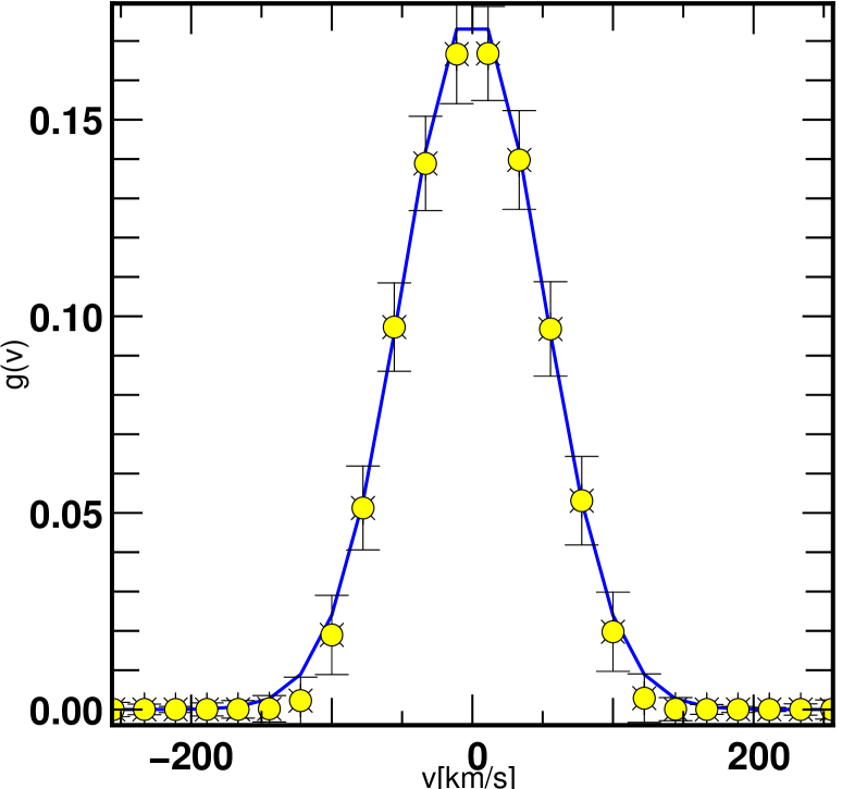
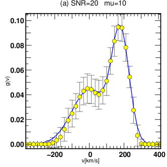
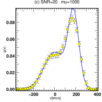
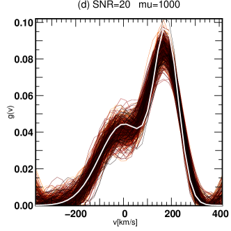
We applied this deconvolution technique to mock data, created from Pégase-HR SSPs of several ages and metallicities, with $R=10\,000$ at $4000-6800$ Å. In a first set of experiments, the model spectrum at rest was a solar metallicity $10$ Gyr single stellar population. It was convolved with various LOSVDs, both Gaussian and non Gaussian, with velocity dispersions ranging from $30$ to $500$ km/s. It was then perturbed with Gaussian noise at levels ranging from SNR$=5$ to $100$ per pixel, and deconvolved using the model spectrum at rest as template (i.e. no template mismatch). In all cases, the LOSVDs are adequately recovered. Figure 1 shows the reconstruction of a Gaussian LOSVD, for SNR$=10$ per pixel. However, there are necessarily some biases in the reconstruction of the sharp features of the LOSVD. This is expected since we introduced regularization via smoothing. To illustrate the relationship between regularization and bias, we performed a new set of similar simulations for a non-Gaussian LOSVD (sum of 2 Gaussians) with SNR=20 per pixel and varied the smoothing parameter $\mu$. The results are shown in figure 2. The panels a and b correspond to $\mu=10$ while the panels c and d correspond to $\mu=1000$. The model, median and interquartiles of 500 reconstructions are displayed. We also plotted the whole set of 500 recovered solutions, in order to show the locus of the solutions. One can see that the biases of the median recontruction are reduced when lowering $\mu$. The highest bump is correctly reproduced for $\mu=10$ while it is not for $\mu=1000$. But on the other hand the solutions are much more widely spread when $\mu=10$. This means that most solutions taken from the set of low $\mu$ simulations can be very far from the model, while all the large $\mu$ solutions lie reasonably close to the model.

The regularization acts as a Wiener filter in the sense that it damps the high frequency components of the solution. Regularization improves the significance of an individual reconstruction (it will nearly always lie reasonably close to the model), at the cost of introducing a bias.

Figure 1: Non parametric reconstruction of a Gaussian LOSVD for simulated data, $\sigma_{v}=100$ km/s, SNR=10 per pixel. The model spectrum at rest is a $10$ Gyr old solar metallicity single stellar population with $R=10\,000$ at $4000-6800$ Å. The template spectrum is identical, so that no template mismatch is allowed here. The thick line is the input model. The circles and the bars show respectively the median and the interquartiles of the recovered solutions for 500 realizations of the noise.

Figure 2: Impact of the smoothing parameter. Reconstruction of a non-Gaussian LOSVD for simulated data with SNR=20 per pixel. Top: $\mu=10$, bottom: $\mu=1000$. Left: the thick line is the input model LOSVD. The circles and the bars show respectively the median and interquartiles of the reconstructed LOSVDs for 500 realizations of the experiment. Right: the whole set of 500 solutions is displayed, with the model as a thick white line, in order to give the reader a sense of what individual solutions look like. The figures show the tradeoff between bias and reliability of the reconstruction: for small $\mu$ the median reconstruction is unbiased but the individual reconstructions are very noisy. For large $\mu$ the median reconstruction is slightly biased but all the reconstructions are reasonable. Hence, the significance of an individual reconstruction is improved by regularization at the cost of introducing a bias.

3.4 Age and metallicity mismatch

We take advantage of the large range of ages and metallicities of single stellar populations covered by Pégase-HR to shortly illustrate the effects of template mismatch on LOSVD determinations. In this section we show the results of a large number of simulations aiming at characterizing the error made when a wrong template is chosen for the kinematical inversion of data. For this purpose, mock data were created by convolving a single stellar population of age, $a_{0}$, and metallicity, $Z_{0}$, with a centered Gaussian LOSVD of dispersion $\sigma_{v}=50$ km/s. It was perturbed by Gaussian noise corresponding to SNR$=100$ per pixel and then deconvolved, using as template a single stellar population of age $a_{1}$, and metallicity $Z_{1}$. The spectral resolution and wavelength range are the same as in Sect. 3.3. Fig. 3 shows the error on the measured velocity dispersion. The latter is measured as the r.m.s of the reconstructed LOSVD. If the parameters of the template are different from those of the model, the velocity dispersion error increases very quickly. The age metallicity degeneracy is visible as a valley of smaller error, following the upper-left to bottom-right diagonal of the figures. Of course, the $\chi^{2}$ distance between the model and the mock data follows a similar 2D distribution, and will lead to the rejection of highly mismatched LOSVD estimates. However, in practice, it is usually not straightforward to quantify all the sources of error. It is thus somewhat arbitrary to set an upper limit of $\chi^{2}$ for the admissible solutions, and the error on the kinematics is thus hard to quantify. This experiment illustrates in this context the long known issue that when the correct model is not available, large errors on the determination of kinematics are expected. In order to reduce the error in the estimates of the kinematical properties of a stellar assembly, it is necessary to allow for a wide range of modulations of the template. This is naturally achieved by making the non parametric stellar content account for the changes of the template, as discussed in the next section.

Figure 3: Velocity dispersion error as a function of the age and metallicity of the template single stellar population. Contours show regions of increasing velocity dispersion error. In each experiment, the age and metallicity of the original model template is shown as a thick cross, and the model LOSVD is a Gaussian with zero mean and $50$ km/s dispersion. The velocity dispersion error is minimum when the template’s age and metallicity are similar to the model’s. The error increases quickly when the template’s parameters differ from the model’s, also in the age-metallicity degeneracy direction (upper left-bottom right diagonal). It increases even faster in the direction orthogonal to the age-metallicity degeneracy.

4 Recovering stellar content and global kinematics

The mixed inversion described in this section couples the recovery of both the stellar content and the kinematics, thereby turning STECMAP into STECKMAP. Proper application of this method provides an interpretation of the observed object in terms of stellar content and kinematics.

4.1 Inverse problem

For a given model spectrum at rest, $F_{\mathrm{rest}}(\lambda)$, and a LOSVD, $g(v)$, the emitted SED, $\phi(\lambda)$ is given by Eq. (2). We now wish to account also for the additional variables involved in $F_{\mathrm{rest}}$, given by Eq. (1), namely the stellar age distribution, $\Lambda(t)$, the age-metallicity relation $Z(t)$, and the color excess $E(B-V)=E$. Injecting Eq. (1) into the convolution Eq. (3) yields the emitted SED:

$$\phi(w)=\!\iint\!\!f_{\mathrm{ext}}(E,w-u)\Lambda(t)B(w-u,t,Z(t))g(u)\,\mathrm{d}t\,\mathrm{d}u\,,$$ (23)

Solving Eq. (23) for $\Lambda$, $Z$, $E$ and $g$ when $\phi$, $f_{\mathrm{ext}}$ and $B$ are given is the inverse problem we are tackling here.

4.2 Discretization and parameters

Expanding the two time-dependent unknowns $\Lambda(t)$ and $Z(t)$ as a sum of $n$ gate functions and injecting into Eq. (1) yields the discrete model spectrum at rest:

$${{\mathbf{F}}}=\mathrm{diag}(\mathbf{f}_{\mathrm{ext}}(E))\cdot{\mathbf{B\cdot x}}\,,$$ (24)

This discretization is explained in details in Sec.5 of Paper I. Similarly, we develop the LOSVD $g(u)$ as a sum of $p$ gate funtions as in Sect. 3. Note that the reddened model at rest plays the role of the stellar template in a classical kinematic convolution. Injecting Eq. (24) into Eq. (17) thus allows us to express the model spectrum, ${\mathbf{s}}$, as

$${\mathbf{s}}={\cal{F}}^{\ast}\cdot\mathrm{diag}({\cal{F}}\cdot\mathrm{diag}(\mathbf{f}_{\mathrm{ext}}(E))\cdot{\mathbf{B\cdot x}})\cdot{\cal{F}}\cdot{\mathbf{g}}\,,$$ (25)

However, here, the template is this time modulated by the unknowns describing the stellar content.

4.3 Smoothness and metallicity constraints

The discrete problem of finding the stellar age distribution ${\mathbf{x}}$, the age-metallicity relation ${\mathbf{Z}}$, the extinction $E$ and the LOSVD ${\mathbf{g}}$ for an observed spectrum ${\mathbf{y}}$ and given an extinction law $f_{\mathrm{ext}}$ and a SSP basis $B$ is of course likely to be very ill-conditioned since it arises as the combination of several ill-conditioned problems. It therefore requires regularization. We also want the metallicity of the components to remain in the model range. We use the standard penalization $P$ and the binding function $C$ defined in Paper I to build the penalization $P_{\bm{\mu}}$ for this problem:

$$P_{\bm{\mu}}=\mu_{{\mathbf{x}}}P({\mathbf{x}})+\mu_{{\mathbf{Z}}}P({\mathbf{Z}})+\mu_{C}C({\mathbf{Z}})+\mu_{v}P({\mathbf{g}})\,,$$ (26)

where ${\bm{\mu}}\equiv(\mu_{\mathbf{x}},\mu_{\mathbf{Z}},\mu_{C},\mu_{v})$. Again, we choose ${\mathbf{L=D}}_{2}$ as defined in Pichon et al. (2002), so that the penalization $P$ is actually Laplacian. The objective function, $Q_{\bm{\mu}}$, is now defined as:

$$Q_{\bm{\mu}}=\chi^{2}({\mathbf{s}}({\mathbf{x,Z,}}E,{\mathbf{g}}))+P_{\bm{\mu}}({\mathbf{x,Z}},E,{\mathbf{g}})\,.$$ (27)

and its partial derivatives are given in Sect. A.2. Note that there is in principle an additionnal formal degeneracy for this inverse problem. If the set $({\mathbf{x,Z}},E,{\mathbf{g}})$ is a solution to (23), then $(\alpha{\mathbf{x,Z}},E,{\mathbf{g}}/\alpha)$ is also a solution for any scalar $\alpha$, because the age distribution ${\mathbf{x}}$ and the LOSVD ${\mathbf{g}}$ are not explicitly normalized in this formulation. However, the adopted regularization lifts this degeneracy. The penalization function $P$ is quadratic ($P(\alpha{\mathbf{x}})=\alpha^{2}P({\mathbf{x}})$). Thus, if ${\mathbf{x}}$ or ${\mathbf{g}}$ is too large in norm, the solution is unattractive. Practically, the algorithm reaches a solution where ${\mathbf{x}}$ and ${\mathbf{g}}$ are similar in norm. In any case, this degeneracy would easily be remedied by adding a normalizing term to the penalization $P_{\bm{\mu}}$ of the form $\|{\mathbf{x}}\|-1$, which would force the discretized stellar age distribution ${\mathbf{x}}$ to have unitary norm. Following the same principle, one could equivalently choose to normalize the LOSVD rather than the stellar age distribution.

4.4 Simulations

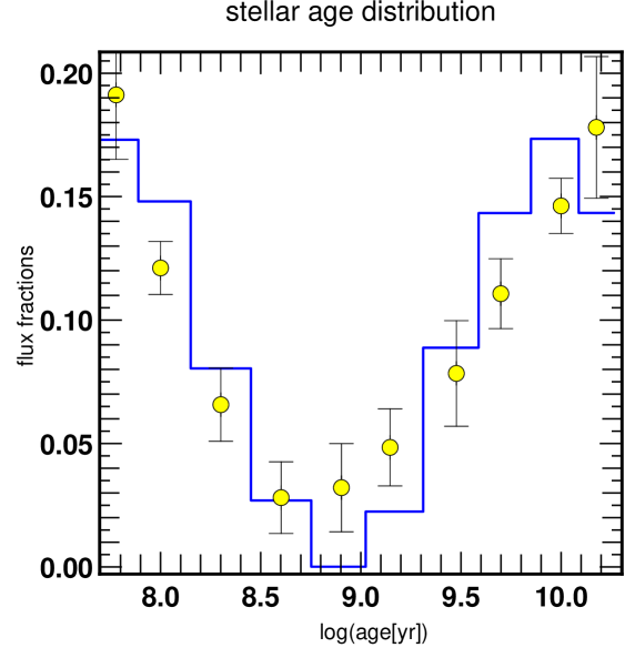
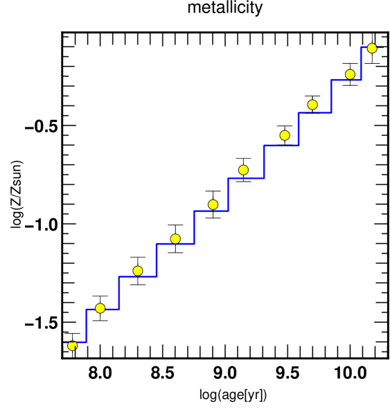
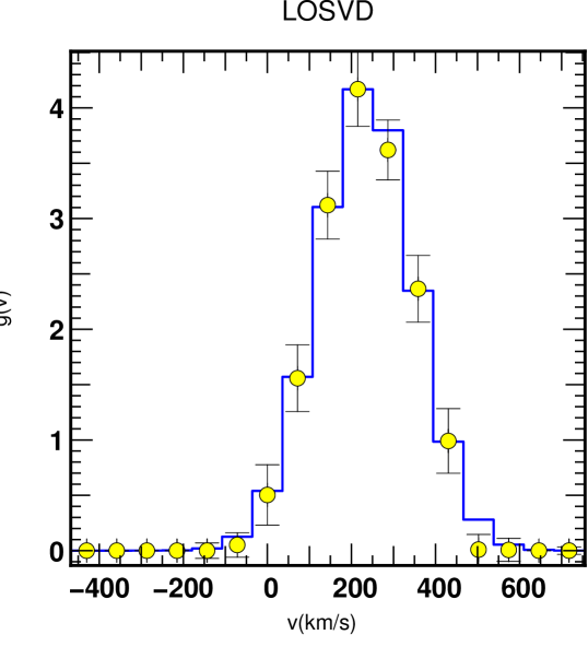
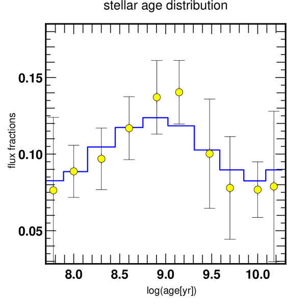
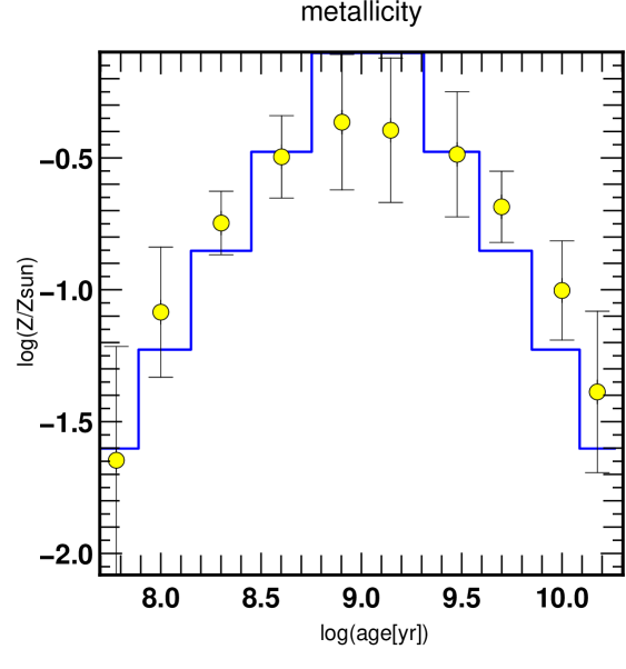
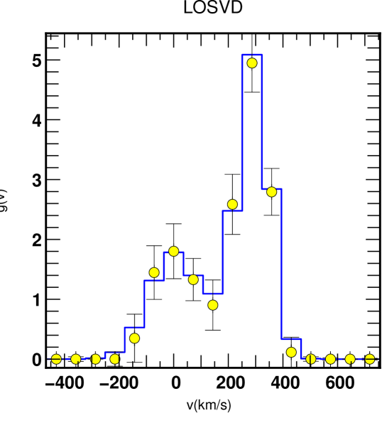
Let us now test the behaviour of STECKMAP by applying it to mock data. The latter were produced using an arbitrary stellar age distribution ${\mathbf{x}}$, an age-metallicity relation ${\mathbf{Z}}$, a LOSVD ${\mathbf{g}}$ and an extinction parameter $E$. Several simulations were performed with various input models: bumpy age distributions, increasing or decreasing age-metallicity relation and extinctions, Gaussian and non Gaussian wide or narrow LOSVDs, in various pseudo-observational contexts. Figure 4 shows the results of two of these experiments. In the top line, the model is a young metal-poor population superimposed to an older metal-rich population. In the bottom panels, the model has a rather constant stellar age distribution, a non-monotonic age-metallicity relation and a strongly non Gaussian LOSVD. In both cases the 3 unknowns are correctly recovered. In these examples, the data quality mimics that of the best Sloan Digital Sky Survey galaxies: the resolution is $R\approx 2000$ and SNR$=30$ per $\approx$1 Å pixel. The wavelength domain of Pégase-HR is however narrower than the SDSS’s. These simulations simply aim at demonstrating the generally good behaviour of the method, and show that accounting for the kinematics does not fundamentally weaken the constraints on the stellar content. For a more thorough study of the informational content of the Pégase-HR wavelength range, the reader can refer to the systematic double burst simulations with variable spectral resolution and SNR per Å performed in Paper I.

Figure 4: Reconstruction of the stellar age distribution, age-metallicity relation and LOSVD for simulated SDSS-like data with SNR=30 per pixel. The thick histogram is the input model. The circles and the bars show respectively the median and the interquartiles of the recovered solutions for 50 realizations.

5 Recovery of age-dependent kinematics

In this section we present an implementation of the recovery of age-dependent kinematics, i.e the situation when each sub-population has its own LOSVD. In this experiment, we restrict ourselves to the case where the stellar populations have a known metallicity and are seen without extinction. This choice is mainly motivated by the numerical cost of such a large inversion procedure. The modeling is given by Eq. (10). Finding the age-velocity distribution ${\Xi}(u,t)$ when the mono-metallic basis $B$ and the observed spectrum $\phi$ are given is the inverse problem. It arises as the combination of a linear age inversion and a kinematical deconvolution.

5.1 A sum of convolutions

The age-velocity distribution, ${\Xi}(u,t)$, is expanded as a linear combination of normalized 2D gate functions $\theta_{ij}(u,t)$:

$$\theta_{ij}(u,t)\equiv\frac{1}{\delta{}u\,\delta{}t}\,\theta\left(\frac{u-u_{i}}{\delta{}u}\right)\,\theta\left(\frac{t-t_{j}}{\delta{}t}\right)\,.$$

In other words, ${\Xi}(u,t)$ is represented by a 2D array ${\mathbf{v}}$ of size $(p,n)$, i.e. $p$ is the size of each LOSVD and $n$ is the number of age bins. The linear step in $u$ is $\delta u$ and the step in $t$ is $\delta t$.

By injecting the expansion into Eq. (10) we obtain

$$\phi(w) = \iint\sum_{i=1}^{p}\sum_{j=1}^{n}v_{ij}\theta_{ij}(u,t)B(w-u,t)\mathrm{d}t\mathrm{d}u\,,$$ (28)

$$\simeq \sum_{i=1}^{p}\sum_{j=1}^{n}v_{ij}B_{j}(w-u_{i})\,.$$

As in the previous sections, $B_{j}(u)$ is a time-averaged single stellar population of age $t_{j}\pm\frac{1}{2}\,\delta{}t$. We then discretize along wavelengths by averaging over small $\delta w$:

$$\phi_{k} = \frac{1}{\delta w}\sum_{i=1}^{p}\sum_{j=1}^{n}v_{ij}\,\int B_{j}(w-u_{i})\,\theta\left(\frac{w-w_{k}}{\delta\,w}\right)\mathrm{d}w\,,$$ (29)

$$\simeq \sum_{i=1}^{p}\sum_{j=1}^{n}v_{ij}\,B_{j}(w_{k}-u_{i})\,,$$

where $(w_{j})_{j\in\{0,...,m\}}$ is a set of constant step logarithmic wavelengths. The above expression also reads in matrix form as a sum of kernel convolutions. Finally, the model SED of the emitted light reads:

$${\mathbf{s}}=\sum_{j=1}^{n}{\mathbf{K}}_{j}\cdot{\mathbf{v}}_{j}\,,$$ (30)

where ${\mathbf{s}}=\left(\phi_{1},\phi_{2},\dots,\phi_{m}\right)$, ${\mathbf{v}}_{j}=\left(v_{1j},v_{2j},\dots,v_{pj}\right)$ and

$${\mathbf{K}}_{j}=\left[\begin{array}[]{rrrr}K_{11j}&K_{12j}&\dots&K_{1pj}\\ K_{21j}&K_{22j}&\dots&K_{2pj}\\ \vdots&\vdots&\ddots&\vdots\\ K_{m1j}&K_{m2j}&\dots&K_{mpj}\end{array}\right]\,,$$ (31)

with

$$K_{ikj}\equiv B_{j}(w_{k}-u_{i})\,.$$ (32)

With this notation, ${\mathbf{K}}_{j}$ and ${\mathbf{v}}_{j}$ are respectively the convolution kernel and the LOSVD of the sub-population of age $t_{j}$, and the model spectrum ${\mathbf{y}}$ is the sum of the convolution of the kernel of each sub-population by its own LOSVD.

5.2 2D age-velocity smoothness constraints

In the previous sections, the unknowns were mono-dimensional functions of time or velocity. Here, the unknown is a 2D distribution, and we thus have to implement a 2D smoothing constraint. We wish to allow the smoothness in age to be distinct from the smoothness in velocity. We thus construct two penalizing functions, $P_{a}$ and $P_{v}$, relying on the standard function $P$. $P_{a}$ computes the sum of the Laplacians of the columns of ${\mathbf{v}}$ while $P_{v}$ computes the sum of the Laplacians of the lines of ${\mathbf{v}}$. The smoothness in the direction of the velocities (respectively ages) is set by $\mu_{v}$ (respectively $\mu_{a}$). We define the vectors ${\mathbf{v}}_{j}=(v_{1j},v_{2j},\cdots,v_{pj})$ as the columns of ${\mathbf{v}}$, i.e. the LOSVD s of the subpopulations. We similarly define the ${\mathbf{v}}^{i}=(v_{i1},v_{i2},\cdots,v_{in})$ as the lines of ${\mathbf{v}}$. With this notation, the penalization $P_{\bm{\mu}}$ reads:

$$P_{\bm{\mu}}({{\mathbf{v}}}) \equiv \mu_{a}P_{a}({{\mathbf{v}}})+\mu_{v}P_{v}({\mathbf{v}})\,,$$ (33)

$$\equiv \mu_{a}\sum_{i=1}^{p}P({{\mathbf{v}}}^{i})+\mu_{v}\sum_{j=1}^{n}P({{\mathbf{v}}}_{j})\,.$$

The objective function, $Q_{\bm{\mu}}$, is now fully specified as $Q_{\bm{\mu}}=\chi^{2}+P_{\bm{\mu}}$. Its gradients are given in appendix A.3. We choose here the smoothing parameters, $\bm{\mu}\equiv(\mu_{a},\mu_{v})$, on the basis of simulations.

5.3 Simulations of a bulge-disk system

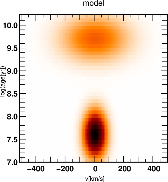
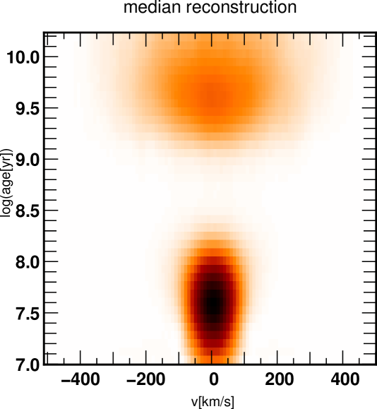
We studied the feasibility of separating two age-dynamically distinct populations, i.e. two components which do not overlap in an age-velocity distribution diagram, in a regime of very high quality model and data. We performed simulations in the idealized case of a very simplified spiral galaxy consisting of a bulge-disk system of solar metallicity seen without extinction at some intermediate inclination, in two observational contexts. The corresponding ages and projected kinematical parameters are given in Table 1. The resolution of the pseudo-data is $R=10\,000$ at $4000-6800$ Å, and the SNR is $100$ per $0.2$ Å pixel.

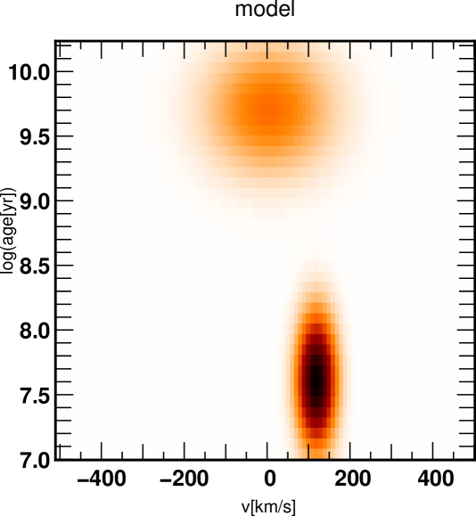
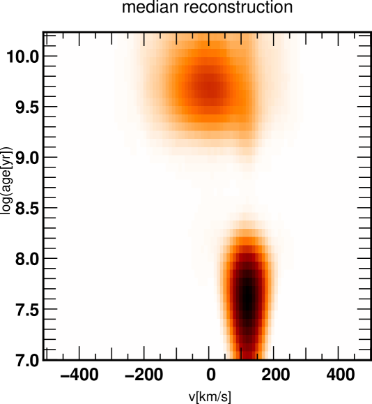
• Case 1: The galaxy is resolved, and the fiber aperture is small compared to the angular size of the galaxy. The line of sight is offset by a couple kpc from the center along the major axis. The projected model age-velocity distribution involves 2 superimposed components: an old, non-rotating kinematically hot population representing the bulge, and a young, rotating, kinematically cold component. The model and the median of 30 reconstructions are shown in Fig. 5. The separation of the components is clear and their parameters can be recovered with good accuracy, considering the difficulty of the task.

• Case 2: The galaxy is unresolved. The difference with the former situation is that because of the spatial integration, both age-velocity distributions are centered. For a given dynamical model, the projected dispersion of the disk component depends on its inclination. Fig. 6 shows that the separation is successful and that the ages and integrated kinematical properties of both components can be measured.

	$V_{c}(\rm{km/s})$	$\sigma_{\rm{v}}(\rm{km/s})$	age (Gyr)
Case 1
Bulge	0	100	8
Disk	120	30	0.5
Case 2
Bulge	0	150	8
Disk	0	50	0.5

Table 1: Projected kinematical parameters and age of the model bulge-disk system used to produce the simulations of Fig. 5 and Fig. 6. $V_{c}$ (respectively $\sigma_{\rm{v}}$) is the rotation velocity (respectively the velocity dispersion) projected on the line of sight.

Figure 5: Model (left) and median reconstruction (right, $\approx$ 30 realizations) of a stellar age-velocity distribution from SNR$=$100 per $0.2$ Å pixel pseudo-data at 4000$-$6800 Å. The model stellar age-velocity distribution mimics that of a simplified spiral galaxy seen with intermediate inclination. The old broad component can account for the bulge population while the young narrow rotating component represents a thin disk population. The projected kinematical parameters of the model are given in Table 1 (case 1). The different kinematical components are well separated and clearly identifiable.

Figure 6: Same as Fig. 5 but for an unresolved simplified spiral galaxy with projected and spatially integrated kinematical parameters given in Table 1 (case 2). The velocity dispersion of the integrated young disc component depends on the inclination angle. The bulge and the disc are are well separated and clearly identifiable. Their respective velocity dispersions and ages are reliably recovered.

6 Conclusions

The non-parametric kinematical deconvolution of a galaxy spectrum is efficiently performed using a MAP formalism (Sect. 3). Regularization through smoothness requirements and positivity improve significantly the behaviour of the inversion with respect to noise in the data. This improvement occurs at the cost of introducing some bias in the reconstructed LOSVD, but this bias remains reasonable. Strong non-Gaussianities of LOSVDs are reliably detected from mock data generated using Pégase-HR SSPs for SNR down to $20$ per $0.2$ Å pixel.

When the template does not exactly match the model spectrum at rest, i.e. there is some template mismatch, the error on the velocity dispersion increases very quickly (Sect. 3.4). For example, in our experiments, where $\sigma_{\rm{V}}=50$ km/s with $R=10\,000$ data, the error on the measured velocity dispersion amounts up to 10-20 per cent if the template differs from the model by more than 0.3 dex in age and metallicity, perpendicular to the age-metallicity degeneracy.

The formal similarity between the non-parametric kinematical deconvolution and the recovery of the stellar content allows us to merge both processes in a “mixed” inversion where the observed spectrum is fitted by determining the stellar content and the kinematics simultaneously (Sect. 4). This circumvents the need for iterations where kinematical and stellar content analyses are carried out one after the other, until convergence is reached; this provides an efficient method to analyze large sets of data.

Satisfactory reconstructions of the stellar age distribution, the age-metallicity relation, the extinction and the global LOSVD were obtained from mock data down to $R=2000$, SNR$=30$ per 1 Å pixel in the $4\,000-6\,800$ Å range (simulating SDSS data in the Pégase-HR range), indicating the good behaviour of the method. Since in our simulations, the introduction of the kinematics into STECMAP did not affect the recovery of the stellar content, we consider that the error estimates and separability analysis given in Paper I remain valid.

In a more exploratory part of this work, we showed the feasibility of recovering age-dependent kinematics in a simplified mono-metallic unreddened context (Sect. 5). We were able to separate the bulge and disc component of a simplified model spiral galaxy in integrated light provided very high quality data (SNR=100 per $0.2$ Å pixel in the optical domain) and models are available, i.e. we constrain both components in velocity dispersion and age. This separation was also carried out successfully in the setup corresponding to an unresolved galaxy.

Further investigations are needed to extend this technique to a regime where the metallicity and extinction are unknown. We expect that letting the metallicity be a free parameter would certainly lead to a more degenerate problem, as shows the degradation of the resolution in age found in Paper I compared to fixed metallicity problems. On the contrary, we do not expect the addition of the extinction as a free parameter or a more complex form of extiction law or flux calibration correction, possibly non parametric, to deteriorate the conditioning of the problem. The results are encouraging, and the feasibility of such age-dependent kinematics reconstructions deserves to be tackled in realistic specific pseudo-observational regimes in the future.

As mentioned in Paper I, the SSP models were considered to be perfect and noiseless. It still has to be investigated how instrumental error sources such as flux and wavelength calibration error, additive noise, contamination by adjacent objects, and, equally important, model errors, can affect the robustness of such sophisticated interpretations.

Perspectives

STECKMAP will be very useful to interpret data of large spectroscopic surveys, complete or in progress, such as 2DFGRS, SDSS, DEEP2, or VVDS, especially where both constraints on the stellar content and the dynamics are required. STECKMAP’s analysis of the spectroscopic survey data or of a SNR selected subsample, combined with survey photometry could provide estimates of the stellar and dynamical masses (which must be corrected for fiber aperture though), thereby allowing astronomers the prospect of investigating the dark matter content in galaxies on a statistically significant sample, in the spirit of Padmanabhan et al. (2004).

The application of age-dependent kinematics to integral field spectroscopy data from, for example SAURON (Bacon et al., 2001; de Zeeuw et al., 2002), OASIS (McDermid et al., 2004), MUSE (Henault et al., 2003) or MPFS (Chilingarian et al., 2004) could significantly boost the amount of information extracted from this data.

The inner parts of elliptical or dwarf elliptical galaxies have shown via adaptive optics new kinematically decoupled structures (cores or central disks), which were precedently unresolved (McDermid et al., 2004; Bacon et al., 2001). Similarly, if decoupled structures are unresolved and remain so, even with adaptive optics, it may still be possible to separate components in age-velocity space. Hence, the technique presented in Sect. 5 extends the range of investigation for the inner components of galaxies even further in redshift and distance with the current generation of instruments. The faint, generalized counterparts of kinematically decoupled cores, i.e. stellar streams generated by minor merging and accretion of satellites, may also be detectable by an age-dependent kinematics reconstruction in systems which can not be resolved into stars, provided that they are sufficiently distinct from the bulk stars of the galaxy in the age-velocity space. This will enlarge the sample of galaxies for which such detailed information is available, and may make it statistically significant.

Acknowledgments

We are grateful to A. Siebert for useful comments and helpful suggestions. We would like to thank D. Munro for freely distributing his Yorick programming language (available at http://www.maumae.net/yorick/doc/index.html), together with its MPI interface, which we used to implement our algorithm in parallel. PO thanks the MPA for their hospitality and funding from a Marie Curie studentship.

Appendix A Gradient computations

A.1 Kinematic deconvolution

In this section we derive the gradient of $Q_{\mu}$ with respect to the LOSVD ${\mathbf{g}}$. First, we rewrite the $\chi^{2}$ term as:

$$\chi^{2}={{{\mathbf{r}}}^{\top}}\cdot{\mathbf{W}}\cdot{\mathbf{r}}\,,$$ (34)

where the residuals vector ${\mathbf{r}}$ is defined by

$${\mathbf{r}}={\mathbf{y}}-{{\cal{F}}}^{-1}\cdot\mathrm{diag}({\cal{F}}\cdot{\mathbf{F}})\cdot{\cal{F}}\cdot{\mathbf{g}}\,,$$ (35)

The derivative of the $\chi^{2}$ then reads:

$$\frac{\partial\chi^{2}}{\partial{\mathbf{g}}}=-2{\cal{F}}^{\ast}\cdot\mathrm{diag}({\cal{F}}\cdot{\mathbf{F}})^{\ast}\cdot{\cal{F}}\cdot{\mathbf{W\cdot r}}\,,$$ (36)

where the asterisk $\ast$ denotes the complex conjugate. Since the stellar template and the LOSVD can play symmetrical roles in Eq. (17) we can also write the derivative of ${\chi^{2}}$ relatively to the stellar template:

$$\frac{\partial\chi^{2}}{\partial{\mathbf{F}}}=-2{\cal{F}}^{\ast}\cdot\mathrm{diag}({\cal{F}}\cdot{\mathbf{g}})^{\ast}\cdot{\cal{F}}\cdot{\mathbf{W\cdot r}}\,,$$ (37)

This expression will be useful for later derivations of gradients for more complex problems in the following appendices.

A.2 Gradients of the mixed inversion

Here we show how to obtain the partial derivatives of $Q_{\mu}=\chi^{2}+P_{\mu}$ as defined in Sect. 4. Given that writing the derivatives of the penalizing functions $P_{\mu}$ is straightforward, we will in this appendix focus on the gradients of the $\chi^{2}$. In the mixed inversion, the reddened model spectrum at rest plays the role of the stellar template ${\mathbf{F}}$ in the classical kinematic deconvolution of equation (15). $\partial\chi^{2}/\partial{\mathbf{g}}$ can thus be obtained by replacing ${\mathbf{F}}\leftarrow\mathrm{diag}(\mathbf{f}_{\mathrm{ext}}(E))\cdot{\mathbf{B\cdot x}}$ in equation (36).

$$\frac{\partial\chi^{2}}{\partial{\mathbf{g}}}=-2{\cal{F}}^{\ast}\cdot\mathrm{diag}({\cal{F}}\cdot\mathrm{diag}(\mathbf{f}_{\mathrm{ext}}(E))\cdot{\mathbf{B\cdot x}})^{\ast}\cdot{\cal{F}}\cdot{\mathbf{W\cdot r}}\,,$$ (38)

where ${\mathbf{r}}={{\mathbf{y-s}}}$ is the residuals vector, with ${\mathbf{s}}$ as given by Eq. (25). To obtain the other partial derivatives we use the following relation. For any parameter $\alpha$ we have

$$\frac{\partial{\chi^{2}}}{\partial\alpha}={{\left(\frac{\partial{\chi^{2}}}{\partial{\mathbf{F}}}\right)}^{\top}}\cdot\frac{\partial{\mathbf{F}}}{\partial\alpha}\,.$$ (39)

The first term $\partial\chi^{2}/\partial{\mathbf{F}}$ is given by Eq. (37) while the second term reads, considering each unknown:

$$\frac{\partial{\mathbf{F}}}{\partial{\mathbf{x}}} = \mathrm{diag}(\mathbf{f}_{\mathrm{ext}})\cdot{\mathbf{A}}\,,$$ (40)

$$\frac{\partial{\mathbf{F}}}{\partial{\mathbf{Z}}} = \mathrm{diag}({\mathbf{x}})\cdot\frac{\partial{\mathbf{B}}}{\partial{\mathbf{Z}}}\cdot\mathrm{diag}(\mathbf{f}_{\mathrm{ext}})\,,$$ (41)

$$\frac{\partial{\mathbf{F}}}{\partial{E}} = \mathrm{diag}(\frac{\partial\mathbf{f}_{\mathrm{ext}}}{\partial E})\cdot{\mathbf{A}}\cdot{\mathbf{x}}\,,$$ (42)

with the same notation as in the appendix of the STECMAP paper.

A.3 Gradients for the age-dependent kinematics recovery

Again, we focus on the partial derivatives of the $\chi^{2}$. Using Eq. (17), the model can be rewritten using the Fourier operator

$${\mathbf{s}}=\sum_{j=1}^{n}{\cal{F}}^{\ast}\cdot\mathrm{diag}({\cal{F}}\cdot{\mathbf{B}}_{j})\cdot{\cal{F}}\cdot{\mathbf{v}}_{j}\,,$$ (43)

where ${\mathbf{B_{j}}}$ is the discretized time-averaged single stellar population of age $[t_{j-1},t_{j}]$, The derivatives of $\chi^{2}$ relatively to ${\mathbf{v}}$ can be derived directly from Eq. (36) since the model is just a sum of convolutions. Replacing ${\mathbf{F}}\leftarrow{\mathbf{B}}_{j}$ and ${\mathbf{g}}\leftarrow{\mathbf{v}}_{j}$ yields the gradient of the $\chi^{2}$:

$$\frac{\partial\chi^{2}}{\partial{\mathbf{v}}_{j}}=-2{\cal{F}}^{\ast}\cdot\mathrm{diag}({\cal{F}}\cdot{\mathbf{F}})^{\ast}\cdot{\cal{F}}\cdot{\mathbf{W\cdot r}}\,,$$ (44)

with the residuals vector ${\mathbf{r=y-s}}$. Finally, the derivative of $Q_{\mu}$ relatively to ${\mathbf{v}}$ is the matrix defined by

$$\frac{\partial Q_{\mu}}{\partial{\mathbf{v}}}=\left(\frac{\partial Q_{\mu}}{\partial{\mathbf{v}}_{1}}\,,\frac{\partial Q_{\mu}}{\partial{\mathbf{v}}_{2}}\,\dots\,\frac{\partial Q_{\mu}}{\partial{\mathbf{v}}_{n}}\right)\,.$$ (45)

References

- Bacon et al. (2001) Bacon R., Copin Y., Monnet G., Miller B. W., Allington-Smith J. R., Bureau M., Marcella Carollo C., Davies R. L., Emsellem E., Kuntschner H., Peletier R. F., Verolme E. K., Tim de Zeeuw P., 2001, MNRAS , 326, 23
- Bacon et al. (2001) Bacon R., Emsellem E., Combes F., Copin Y., Monnet G., Martin P., 2001, A&A , 371, 409
- Balcells & Quinn (1990) Balcells M., Quinn P. J., 1990, ApJ , 361, 381
- Bender (1990) Bender R., 1990, A&A , 229, 441
- Bender & Surma (1992) Bender R., Surma P., 1992, A&A , 258, 250
- Calzetti (2001) Calzetti D., 2001, PASP , 113, 1449
- Cappellari & Emsellem (2004) Cappellari M., Emsellem E., 2004, PASP , 116, 138
- Chilingarian et al. (2004) Chilingarian I., Prugniel P., Silchenko O., Afanasiev A., 2004, astro-ph/0412293
- Davies et al. (1993) Davies R. L., Sadler E. M., Peletier R. F., 1993, MNRAS , 262, 650
- De Bruyne et al. (2004a) De Bruyne V., De Rijcke S., Dejonghe H., Zeilinger W. W., 2004a, MNRAS , 349, 440
- De Bruyne et al. (2004b) De Bruyne V., De Rijcke S., Dejonghe H., Zeilinger W. W., 2004b, MNRAS , 349, 461
- De Rijcke et al. (2004) De Rijcke S., Dejonghe H., Zeilinger W. W., Hau G. K. T., 2004, A&A , 426, 53
- de Zeeuw et al. (2002) de Zeeuw P. T., Bureau M., Emsellem E., Bacon R., Marcella Carollo C., Copin Y., Davies R. L., Kuntschner H., Miller B. W., Monnet G., Peletier R. F., Verolme E. K., 2002, MNRAS , 329, 513
- Faber et al. (1985) Faber S. M., Friel E. D., Burstein D., Gaskell C. M., 1985, ApJS , 57, 711
- Falcón-Barroso et al. (2003) Falcón-Barroso J., Balcells M., Peletier R. F., Vazdekis A., 2003, A&A , 405, 455
- Ferguson et al. (2002) Ferguson A. M. N., Irwin M. J., Ibata R. A., Lewis G. F., Tanvir N. R., 2002, AJ , 124, 1452
- Freeman & Bland-Hawthorn (2002) Freeman K., Bland-Hawthorn J., 2002, ARAA , 40, 487
- Henault et al. (2003) Henault F., Bacon R., Bonneville C., Boudon D., Davies R. L., Ferruit P., Gilmore G. F., LeFevre O., Lemonnier J., Lilly S., Morris S. L., Prieto E., Steinmetz M., de Zeeuw P. T., 2003, in Instrument Design and Performance for Optical/Infrared Ground-based Telescopes. Edited by Iye, Masanori; Moorwood, Alan F. M. Proceedings of the SPIE, Volume 4841, pp. 1096-1107 (2003). MUSE: a second-generation integral-field spectrograph for the VLT. pp 1096–1107
- Ibata et al. (2004) Ibata R., Chapman S., Ferguson A. M. N., Irwin M., Lewis G., McConnachie A., 2004, MNRAS , 351, 117
- Kroupa et al. (1993) Kroupa P., Tout C. A., Gilmore G., 1993, MNRAS , 262, 545
- Kuijken & Merrifield (1993) Kuijken K., Merrifield M. R., 1993, MNRAS , 264, 712
- Kuntschner (2000) Kuntschner H., 2000, MNRAS , 315, 184
- Kuntschner (2004) Kuntschner H., 2004, A&A , 426, 737
- Le Borgne et al. (2004) Le Borgne D., Rocca-Volmerange B., Prugniel P., Lançon A., Fioc M., Soubiran C., 2004, A&A , 425, 881
- McDermid et al. (2004) McDermid R., Bacon R., Adam G., Benn C., Emsellem E., Cappellari M., Kuntschner H., Bureau M., Copin Y., Davies R. L., Falcon-Barroso J., Ferruit P., Krajnovic D., Peletier R. F., Shapiro K., de Zeeuw P. T., 2004, The Newsletter of the Isaac Newton Group of Telescopes (ING Newsl.), issue no. 8, p. 3., 8, 3
- McDermid et al. (2004) McDermid R., Emsellem E., Cappellari M., Kuntschner H., Bacon R., Bureau M., Copin Y., Davies R. L., Falcón-Barroso J., Ferruit P., Krajnović D., Peletier R. F., Shapiro K., Wernli F., de Zeeuw P. T., 2004, Astronomische Nachrichten, 325, 100
- Merritt (1997) Merritt D., 1997, AJ , 114, 228
- Ocvirk et al. (2005) Ocvirk P., Pichon C., Lancon A., Thiebaut E., 2005, astro-ph/0505209
- Padmanabhan et al. (2004) Padmanabhan N., Seljak U., Strauss M. A., Blanton M. R., Kauffmann G., Schlegel D. J., Tremonti C., Bahcall N. A., Bernardi M., Brinkmann J., Fukugita M., Ivezić vZ., 2004, New Astronomy, 9, 329
- Pichon et al. (2002) Pichon C., Siebert A., Bienaymé O., 2002, MNRAS , 329, 181
- Pinkney et al. (2003) Pinkney J., Gebhardt K., Bender R., Bower G., Dressler A., Faber S. M., Filippenko A. V., Green R., Ho L. C., Kormendy J., Lauer T. R., Magorrian J., Richstone D., Tremaine S., 2003, ApJ , 596, 903
- Press (2002) Press W. H., 2002, Numerical recipes in C++ : the art of scientific computing. Numerical recipes in C++ : the art of scientific computing by William H. Press. ISBN : 0521750334
- Rix & White (1992) Rix H., White S. D. M., 1992, MNRAS , 254, 389
- Saha & Williams (1994) Saha P., Williams T. B., 1994, AJ , 107, 1295
- Trager et al. (1998) Trager S. C., Worthey G., Faber S. M., Burstein D., Gonzalez J. J., 1998, ApJS , 116, 1
- van der Marel & Franx (1993) van der Marel R. P., Franx M., 1993, ApJ , 407, 525
- Wahba (1990) Wahba G., ed. 1990, Spline models for observational data
- Worthey (1994) Worthey G., 1994, ApJS , 95, 107