CORRECTIONS FOR GRAVITATIONAL LENSING OF SUPERNOVAE: BETTER THAN AVERAGE?

Abstract

We investigate the possibility of correcting for the magnification due to gravitational lensing of standard candle sources, such as Type Ia supernovae. Our method uses the observed properties of the foreground galaxies along the lines-of-sight to each source and the accuracy of the lensing correction depends on the quality and depth of these observations as well as the uncertainties in translating the observed luminosities to the matter distribution in the lensing galaxies. The current work is limited to cases where the matter density is dominated by the individual galaxy halos. However, it is straightforward to generalize the method to include also gravitational lensing from cluster scale halos. We show that the dispersion due to lensing for a standard candle source at $z=1.5$ can be reduced from about $7\,\%$ to $\lesssim 3\,\%$, i.e. the magnification correction is useful in reducing the scatter in the Type Ia Hubble diagram, especially at high redshifts where the required long exposure times makes it hard to reach large statistics and the dispersion due to lensing becomes comparable to the intrinsic Type Ia scatter.

1 INTRODUCTION

Observations of high-redshift Type Ia supernovae (SNIa) have in the last decade or so lead to a dramatic paradigm shift in cosmology (Perlmutter et al., 1998; Riess et al., 1998; Schmidt et al., 1998; Perlmutter et al., 1999; Knop et al., 2003; Tonry et al., 2003; Riess et al., 2004). Measurements of the luminosity distance to supernovae over a wide range of redshifts were used to break the degeneracy between cosmic fluids, as suggested by Goobar & Perlmutter (1995). The data clearly favors a universe dominated by repulsive dark energy, and which is presently undergoing accelerated expansion. The next step in observational cosmology is to test the nature of this dark energy, whether constant, i.e. compatible with Einstein’s cosmological constant, or due to completely new physics. Observations of SNIa are among the leading astrophysical tools to explore this question further, as they probe the expansion history of the Universe directly. Large dedicated surveys are in progress (e.g. CFHTLS, ESSENCE, SDSSII) and even more ambitious space based projects are being planned for the future, e.g. the JDEM proposals, DESTINY, JEDI and SNAP.

One thing in common for all these projects is the very large projected number of SNIa that eventually will populate the Hubble diagram used to derive cosmological parameters. Clearly, systematic uncertainties will (soon) become the limiting factor. While some of these uncertainties are due to our lack of knowledge of the SNIa physics and intrinsic properties, others stem from possible interactions of the supernova light (rest-frame UV and optical) near the source or along the line-of-sight (l-o-s), e.g. extinction by dust in the host galaxy or intergalactic medium. In this work, we focus on the gravitational interaction of photons along the l-o-s, i.e. gravitational lensing. As supernova surveys become deeper, the measured source fluxes become increasingly more sensitive to the inhomogeneities in the matter distribution of the Universe. In Amanullah, Mörtsell & Goobar (2003), the JDEM/SNAP mission was simulated using the SNOC Monte-Carlo package (Goobar et al., 2002) and it was found that a careful statistical treatment could be used to optimize the fitting of cosmological parameters from the Hubble diagram of SNIa taking into account the (asymmetric) redshift dependent lensing magnification distribution. Lensing on individual SNe have also been studied, in e.g Lewis & Ibata (2001); Mörtsell, Gunnarsson & Goobar (2001); Benítez et al. (2002); Gunnarsson (2004) by modeling the effect from the galaxies close to the l-o-s to the SN.

In this work, we investigate the accuracy to which lensing (de)magnification can be estimated on individual supernovae. For that purpose, we create mock galaxy catalogs with properties (e.g., galaxy magnitudes, redshifts and spectral types) based on luminosity functions derived from observations by Dahlén et al. (2005). Using the brightness of galaxies as a tracer of the gravitational fields along the l-o-s, we use the multiple lens-plane package Q-LET (Gunnarsson, 2004) to investigate the accuracy to which the magnification can be estimated as a function of the survey parameters, assumptions on M/L-ratios and halo shapes. In an accompanying paper (Jönsson et al., 2005), we apply the technique described here to investigate the lensing magnification probability distribution for 33 supernovae in the GOODS survey (Riess et al., 2004; Strolger et al., 2004).

In this paper, we will assume that dark matter halos in individual galaxy halos and small groups are most important for the lensing magnification of supernovae. For cluster size lenses, additional information is needed to model the gravitational potential, e.g., lensing of background galaxies. Though such a generalization of the method is straightforward, in the following we have assumed the uncertainty in the lensing magnification factor for the small fraction of SNe with foreground clusters to be of the same order as SNe with massive foreground galaxies. Also, we assume that the large scale dark matter structures in the Universe is traced by the luminous matter, i.e. that filaments and walls are populated by galaxies. This approach is reasonable as long as the luminous and dark matter are not anti-correlated, see §5.

In §2, we discuss whether one needs to correct for lensing at all. Section §3 describes the underlying theory and §4 treats our method for estimating the accuracy of the lensing corrections. We summarize and discuss our results in §5. Throughout the paper we use natural units, where $c=G=1$. We assume that the underlying cosmological parameters are $H_{0}=70\ {\rm km}\ \!{\rm s}^{-1}{\rm Mpc}^{-1}$, the matter density $\Omega_{\rm M}=0.3$ and the dark energy density $\Omega_{\Lambda}=0.7$. When no explicit redshift dependence is shown, quantities refer to present values ($z=0$). Quoted magnitudes are in the Vega system.

2 TO CORRECT OR NOT TO CORRECT

Since the mean magnification due to gravitational lensing of a large number of sources is expected to be unity relative to a homogeneous universe, the question arises whether one should correct for the effect of gravitational lensing at all.

Because flux, $f$, is conserved, it is the mean of the magnification factor, $\mu$, that is equal to one, i.e. $\bar{\mu}=1$, or defining $\mu=1+\delta$ where $\delta$ is the fractional difference in luminosity from the unlensed (homogeneous universe) case, $\bar{\delta}=0$. The magnitude is given by $m=-2.5\log f+{\rm const}$, and we can write

$$m=m_{0}-\frac{2.5}{\ln 10}\ln\mu,$$ (1)

where $m_{0}$ is the unlensed magnitude. Taylor expanding $\ln\mu=\ln(1+\delta)$, we get

$$m=m_{0}-\frac{2.5}{\ln 10}\left[\delta-\frac{\delta^{2}}{2}+{\mathcal{O}}(\delta^{3})\right],$$ (2)

with mean value $\bar{m}=m_{0}+0.54\bar{\delta^{2}}+{\mathcal{O}}(\bar{\delta^{3}})$. From this it is clear that the average lensed magnitude need not be equal to the unlensed magnitude. Note that in current surveys, this effect is very small compared to, e.g., the intrinsic scatter of SN luminosities which is why the distinction is still unimportant. Note also that the mean magnification factor is unity only for random source positions. For an actual sample of observed SNIa, magnification bias can push the mean magnification to higher values.

However, given that we have a sample of random source position SNIa and neglect the small corrections to $\bar{m}$ (or perform our cosmology fit using flux units), then $\bar{m}$ is an unbiased estimator for the population mean of the observed magnitudes. Under these circumstances, neglecting the scatter due to lensing does not cause any bias in the fitted cosmological parameters and good statistics will help in beating down the error (e.g., Holz & Linder, 2004). There could still be good reasons to consider correcting for lensing effects. If we are able to reduce the scatter in the observed magnitudes and keep $\bar{m}$ as an unbiased estimator, then we are able to make more accurate cosmology fits. There are also cases where it is non-trivial to quantify the importance of the magnification bias, e.g., the case of SN 1997ff. In a similar context, the ability to correct individual lines-of-sight for gravitational lensing magnification would have a profound impact in our ability use gravitational wave “sirens” for measuring cosmological parameters, as their use as standard candles is ultimately limited by the lensing uncertainty (Holz & Hughes, 2005).

3 MODELING AN INHOMOGENEOUS UNIVERSE

In this section we present a method to investigate the effects of gravitational lensing in an inhomogeneous universe.

3.1 Halo Profiles

Neglecting gravitational lensing is equivalent to assuming that matter is homogeneously distributed in the Universe. However, on small scales, the Universe is certainly inhomogeneous. To investigate the effects of gravitational lensing of distant sources, a realistic model of the matter distribution in the Universe is needed. In the following, we describe how we (re)distribute the matter in our model universe using observations of the luminous matter.

We assume that each galaxy is surrounded by a dark matter halo and that the mass of this halo can be estimated from the galaxy luminosity. However, inferring masses of dark matter halos from luminosities of galaxies is non-trivial. The effects of lensing by a halo depends not only on its mass, but also on its density profile. Both the density profile and mass of dark matter halos are issues under debate. We have chosen to work mainly with two different halo models, Singular Isothermal Spheres (SIS) and the model of Navarro, Frenk and White (NFW; Navarro, Frenk & White, 1997).

The density profile of a SIS, $\rho_{\rm SIS}(r)=\sigma^{2}/(2\pi r^{2})$, is characterized by its l-o-s velocity dispersion $\sigma$, which can be estimated from the galaxy luminosity via the Faber–Jackson (F–J) or Tully–Fisher (T–F) relations, approximately valid for elliptical and spiral galaxies respectively. Since the mass of a SIS halo diverges, $m_{\rm SIS}(r)=2\sigma^{2}r$, we use a truncation radius $r_{\rm t}$. A commonly used scale for halo profiles in general is $r_{\rm 200}$, defined as the radius inside which the mean mass density is 200 times the present critical density. For a SIS halo, $r_{\rm 200}$ and the corresponding mass within this radius, $m_{\rm 200}$, are given by

$$r_{\rm 200}^{\rm SIS}=\frac{\sqrt{2}\sigma}{10H_{0}},\;m_{\rm 200}^{\rm SIS}=\frac{\sqrt{2}\sigma^{3}}{5H_{0}}.$$ (3)

The density profile of a NFW halo is

$$\rho_{\rm NFW}(r)=\frac{\rho_{\rm s}}{(r/r_{\rm s})(1+r/r_{\rm s})^{2}},$$ (4)

where $r_{\rm s}$ is the scale radius for which approximately $\rho_{\rm NFW}\propto r^{-2}$ and $\rho_{\rm s}$ is the density at $r\sim 0.5r_{\rm s}$.

The NFW halo is fully determined by $m_{\rm 200}$ since $r_{\rm 200}=\left[m_{\rm 200}/(100H_{0}^{2})\right]^{1/3}$ and the scale radius $r_{\rm s}$ and $\rho_{\rm s}$ can be found numerically from $m_{\rm 200}$ (Navarro, Frenk & White, 1997).

In the following, we assume that the mass within $r_{\rm 200}$ is roughly the same for the SIS and NFW halo profiles, i.e. $m_{\rm 200}^{\rm SIS}=m_{\rm 200}^{\rm NFW}$. We also set the truncation radius $r_{\rm t}=r_{\rm 200}$ for both SIS and NFW halos. Varying $r_{\rm t}$ does not alter gravitational lensing effects significantly, see §4.5.

3.2 The Smoothness Parameter

Very faint and/or small scale structures cannot all be seen in a magnitude limited survey. Also, for the method used in this paper, any matter not directly associated with individual galaxies such as completely dark halos and cluster halos need to be accounted for. In order to assure that the mean mass density in our model universe is kept constant, we keep the “remaining” mass, not accounted for when relating the dark matter to the luminous matter, as a homogeneous component.

The homogeneous part can be characterized by the smoothness parameter $\eta(z)$, quantifying the fraction of smoothly distributed matter in our model universe (or our lack of knowledge on the dark matter distribution in the real Universe). Since the fraction of galaxies observed at a given magnitude limit is a function of redshift, and also since the Universe evolves, the smoothness parameter is expected to vary with redshift.

The smoothness parameter in a given survey can be computed from the observed density of matter in clumps, i.e. in our case galaxies surrounded by dark matter halos, $\rho_{\rm g}(z)$. If the redshift dependence of $\rho_{\rm g}(z)$ can be factorized into a term $(1+z)^{3}$, scaling like the matter density, and an unknown factor $f(z)$ originating from the magnitude limit of the survey and evolution, we can write

$$\rho_{\rm g}(z)=\rho_{\rm g}(0)(1+z)^{3}f(z).$$ (5)

Then the smoothness parameter is simply given by

$$\eta(z)=1-\frac{\Omega_{\rm G}}{\Omega_{\rm M}}f(z),$$ (6)

where the density in galaxies at $z=0$ has been scaled with the present critical density to $\Omega_{\rm G}$. Once the galaxies have been associated with halos of definite masses, the comoving density of clumps as a function of redshift $\Omega_{\rm G}f(z)$ can be estimated. We divide the distribution of galaxies into redshift bins and estimate $\Omega_{\rm G}f(z)$ in each bin. The density of clumps in the $i$:th bin, centered on redshift $z_{i}$, is obtained through

$$\Omega_{\rm G}f(z_{i})=\frac{1}{\rho_{\rm c}}\frac{\sum_{j}m_{j}}{V_{i}},$$ (7)

where $m_{j}$ is the mass of a clump and $\rho_{\rm c}$ is the critical density. The comoving volume of the $i$:th bin is given by

$$V_{i}=\int_{z_{i}-\Delta z/2}^{z_{i}+\Delta z/2}\frac{D_{\rm A}^{2}(1+z)^{2}}{\left[\Omega_{\rm M}(1+z)^{3}+\Omega_{\Lambda}\right]^{1/2}}{\Delta\Omega}dz,$$ (8)

where $\Delta z$ is the width of the bin, $\Delta\Omega$ is the solid angle under study and $D_{\rm A}$ is the angular diameter distance. Distances have been calculated using the angsiz routines described in Kayser et al. (1997), in which a smoothness parameter varying with redshift can be included. Note that the angular diameter distance $D_{\rm A}$ used to determine the volume element in Eq. (8) above is calculated using the filled-beam approximation ($\eta=1$), since the volume is governed by the global expansion rate, which in turn is governed by the properties on very large scales where the Universe is homogeneous.

3.3 Deriving Velocity Dispersions from Observed Luminosities

Galaxy halo masses can be estimated from the velocity dispersion of galaxies. We calculate the velocity dispersion of each galaxy using absolute magnitudes ($M_{B}$) combined with empirical F–J and T–F relations. For ellipticals, we use the F–J relation

$$\log_{10}\sigma=\log_{10}\sigma_{*}-\frac{0.4}{\gamma}(M_{B}-M_{B}^{*})$$ (9)

where $M_{B}^{*}$ is the characteristic magnitude and $\sigma_{*}$ is the normalization in velocity dispersion. We use $\gamma=4.4$, as derived by Mitchell et al. (2005) using Sloan Digital Sky Survey (SDSS) data. To derive $\sigma_{*}$, we use equation (33) in Mitchell et al. (2005), where we use the relation $M_{r}=M_{B}-1.32$ to convert SDSS $r$–band magnitudes in AB system to standard $B$–band Vega normalized magnitudes. We have here assumed a typical color $M_{B}-M_{r}=1.20$ for ellipticals in the AB-system, and an AB to Vega relation B_AB=B${}_{\rm Vega}-0.12$. The normalization in velocity dispersion is given by

$$\log_{10}\sigma_{*}=2.2-0.091(M_{B}^{*}+19.47+0.85z),$$ (10)

where we use $M_{B}^{*}=-21.04$ derived for the early–type population by Dahlén et al. (2005). Equation (10) yields $\sigma_{*}=220$ ${\rm km\,s^{-1}}$ at $z=0$. Combining equation (9) and (10) gives an expression for the velocity dispersion

$$\log_{10}\sigma=-0.091(M_{B}-4.74+0.85z^{\prime}),$$ (11)

where we use $z^{\prime}=z$ for redshifts $z<1$ and $z^{\prime}=1$ for $z>1$. The redshift dependence of the relation accounts for the brightening of the stellar population with redshift. Since this evolution is poorly known at $z>1$, we assume a flat evolution at these redshifts. As a measurement of the error in the derived relation, we use the observed scatter in the SDSS measurements by Sheth et al. (2003)

$${\rm rms}(\log_{10}\sigma)=0.079[1+0.17(M_{B}+19.705+0.85z^{\prime})],$$ (12)

where we again have transformed SDSS $r$–band to standard $B$–band magnitudes.

For the spiral and later type population, we use the T–F relation derived by Pierce & Tully (1992), with correction for redshift calculated by Böhm et al. (2004)

$$\log_{10}V_{\rm max}=-0.134(M_{B}-\Delta M_{B}+3.52),$$ (13)

where $V_{\rm max}$ is the maximum rotation velocity for the galaxy. The correction due to redshift dependence is

$$\Delta M_{B}=-1.22z^{\prime}-0.09.$$ (14)

The observed scatter in the relation derived by Pierce & Tully (1992) is ${\rm rms}(M_{B})=0.41$, corresponding to

$${\rm rms}(\log_{10}V_{\rm max})=0.06.$$ (15)

At $M_{B}^{*}$, this is similar to the errors in the F–J relation above. Finally, the velocity dispersion in spiral galaxies is related to the circular velocity via $\sigma=V_{\rm max}/\sqrt{2}$.

3.4 Gravitational Lensing with Multiple Lenses

A typical source l-o-s within some angular radius $\theta_{\rm s}$ will contain more than one lens. This requires the multiple lens-plane algorithm (see Schneider, Ehlers & Falco, 1992; Gunnarsson, 2004, for further details), which takes into account each lens along the l-o-s by projecting the lens’ mass distribution onto a plane and then traces the light-ray from the image plane (first lens-plane) back through all lens-planes up to the source plane where the magnification and intrinsic position can be found.

In the following we denote angular diameter distances between redshifts $z_{i}$ and $z_{j}$ by $D_{ij}$. We use $o$ for observer, $s$ for source and $d$ for lens (deflector). When $z_{i}=0$, that index is omitted.

Each halo is truncated in 3D at $r=r_{\rm t}$, then, upon projection onto a plane, the corresponding surface mass density will smoothly go to zero at the projected truncation radius. The projection can be done analytically for our lens models. For simplicity, we start by considering a single lens-plane. The equations can be simplified if we let $\xi$ be the impact parameter on a halo and define $x=\xi/\xi_{0}$ and $x_{\rm t}=r_{\rm t}/\xi_{0}$, where

$$\xi_{0}=\frac{4\pi\sigma^{2}D_{\rm d}D_{\rm ds}}{D_{\rm s}}$$ (16)

for the SIS and

$$\xi_{0}=r_{\rm s}$$ (17)

for the NFW halo. Then, the projected density $\kappa(x)$ can be written as

$$\kappa_{\rm SIS}(x)=\frac{1}{\pi x}\arctan\left(\frac{\sqrt{x_{\rm t}^{2}-x^{2}}}{x}\right)$$ (18)

and

$$\kappa_{\rm NFW}(x)=\frac{2\kappa_{\rm s}}{x^{2}-1}f(x),$$ (19)

where

$$f(x)=\left\{\begin{array}[]{ccc}\frac{\sqrt{x_{\rm t}^{2}-x^{2}}}{1+x_{\rm t}}+\frac{1}{\sqrt{1-x^{2}}}\left({\rm arctanh}\left(\sqrt{\frac{x_{\rm t}^{2}-x^{2}}{1-x^{2}}}\right)-{\rm arctanh}\left(\frac{\sqrt{\frac{x_{\rm t}^{2}-x^{2}}{1-x^{2}}}}{x_{\rm t}}\right)\right)&&x<1<x_{\rm t}\\ \frac{\sqrt{x_{\rm t}^{2}-x^{2}}}{1+x_{\rm t}}+\frac{1}{\sqrt{x^{2}-1}}\left(\arctan\left(\frac{\sqrt{\frac{x_{\rm t}^{2}-x^{2}}{x^{2}-1}}}{x_{\rm t}}\right)-\arctan\left(\sqrt{\frac{x_{\rm t}^{2}-x^{2}}{x^{2}-1}}\right)\right)&&1<x\leq x_{\rm t}\\ \end{array}\right.$$ (20)

and

$$\kappa_{\rm NFW}(1)=\frac{2}{3}\kappa_{\rm s}\left(\frac{x_{\rm t}^{3}-3x_{\rm t}+2}{\left(x_{\rm t}^{2}-1\right)^{\frac{3}{2}}}\right).$$ (21)

Here, $\kappa_{\rm s}=\rho_{\rm s}r_{\rm s}/\Sigma_{\rm cr}$, where $\Sigma_{\rm cr}=D_{\rm s}/4\pi D_{\rm d}D_{\rm ds}$ is a critical density related to strong lensing. Note that $x_{\rm t}>1$ must be assumed for the NFW and that $\kappa=0$ for $x>x_{\rm t}$ for both halo types.

The general expression for the deflection angle for circularly symmetric lenses is

$$\hat{\alpha}(x)=s\alpha(x)=s\frac{2}{x}\int^{x}_{0}x^{\prime}\kappa(x^{\prime})dx^{\prime},$$ (22)

where $s=\xi_{0}D_{\rm s}/D_{\rm d}D_{\rm ds}$, resulting in

$$\alpha(x)=\frac{2}{\pi}\left(\arctan\left(\frac{\sqrt{x_{\rm t}^{2}-x^{2}}}{x}\right)+\frac{x_{\rm t}-\sqrt{x_{\rm t}^{2}-x^{2}}}{x}\right)$$ (23)

for the SIS model. For the NFW halo, numerical evaluation is needed.

As the magnification factor, $\mu^{\prime}$, for all halo models is obtained with distances calculated with the $z$-dependent $\eta$ function, this is the universe relative to which $\mu^{\prime}$ is found (implying $\mu^{\prime}\geq 1$ for primary images). In the following, we will quote magnifications, $\mu$, relative to a universe with homogeneously distributed matter, the filled-beam value (fb) where $\bar{\mu}=1$. The magnifications are related by

$$\mu=\mu^{\prime}\left(\frac{D_{\rm s}^{\rm fb}}{D_{\rm s}^{\eta({\rm z})}}\right)^{2}.$$ (24)

4 SIMULATED SURVEYS

In order to study gravitational lensing corrections, we perform Monte Carlo simulations where we calculate the magnification factor for random source positions in mock galaxy catalogs. By varying the assumptions of the galaxy mass distributions as well as the magnitude limit of the observations, we can estimate the accuracy to which it is possible to correct for the lensing magnification.

For all lensing calculations we have used the publicly available fortran 77 code Q-LET (Gunnarsson, 2004), although substantially modified. The code fully utilizes the multiple lens-plane algorithm and has been used previously by Gunnarsson (2004) and Riess et al. (2004) to study lensing effects on supernovae.

As our simulation base, we create for each Monte Carlo realization a mock galaxy catalog designed to reflect the distribution of galaxies expected in a circular cone around a random l-o-s. To characterize the galaxy population we use the $B$-band rest-frame Schechter luminosity function (LF) derived by Dahlén et al. (2005) using GOODS CDF-S observations. The LF is used to generate the number of expected galaxies within the cone where we take into account Poissonian fluctuations but do not include effects of galaxy correlations or cosmic variance. The same LF is used to assign absolute magnitudes to each object within the range $-23<M_{B}<-16$. To account for evolutionary effects, we include a brightening of the $B$-band characteristic magnitude by $\sim$1 mag to redshift $z=1$ as discussed in §3.3.

A random spectral type is assigned according to the type-specific LF of early-types, late-types and starburst galaxies at $z\sim$0.4 in Dahlén et al. (2005). We thereafter assign early-type galaxies an elliptical morphology and late-type galaxies a spiral morphology. We assume that the fraction of galaxies with elliptical morphology is constant over the redshift range investigated.

The redshift of each object is assigned with a probability proportional to the volume element, $dV(z)/dz$, which is equivalent to assuming a constant comoving number density of galaxies with redshift, i.e. we do not include any evolution of the number densities due to e.g., mergers or large scale structures. The galaxy is finally given a random position within the l-o-s cone.

Besides redshift, absolute magnitude, spectral type and position, we also calculate the apparent magnitude in the observed $I$-band for each object. This allows us to draw subsamples from the catalog with imposed magnitude cutoffs as is the case for real observations. Furthermore, to resemble an observational situation where redshifts are determined photometrically, we also have the option to add a random error to the redshifts. These errors are calculated using simulations and depend on redshift, spectral type and detection S/N. For bright objects with high S/N, errors are typically $\Delta_{z}\equiv\langle|z_{\rm phot}-z_{\rm true}|/(1+z_{\rm spec})\rangle\sim 0.05$, while errors for faint objects (mostly at high $z$) can be as large as $\Delta z\sim 0.3$. The errors for early-type galaxies are typically a factor two smaller compared to late-type galaxies when comparing at the same apparent magnitudes. Besides this ”Gaussian” contribution to the error distribution, a fraction of the galaxies may also be assigned ”catastrophic redshifts” with large errors. We discuss this further in §4.4.

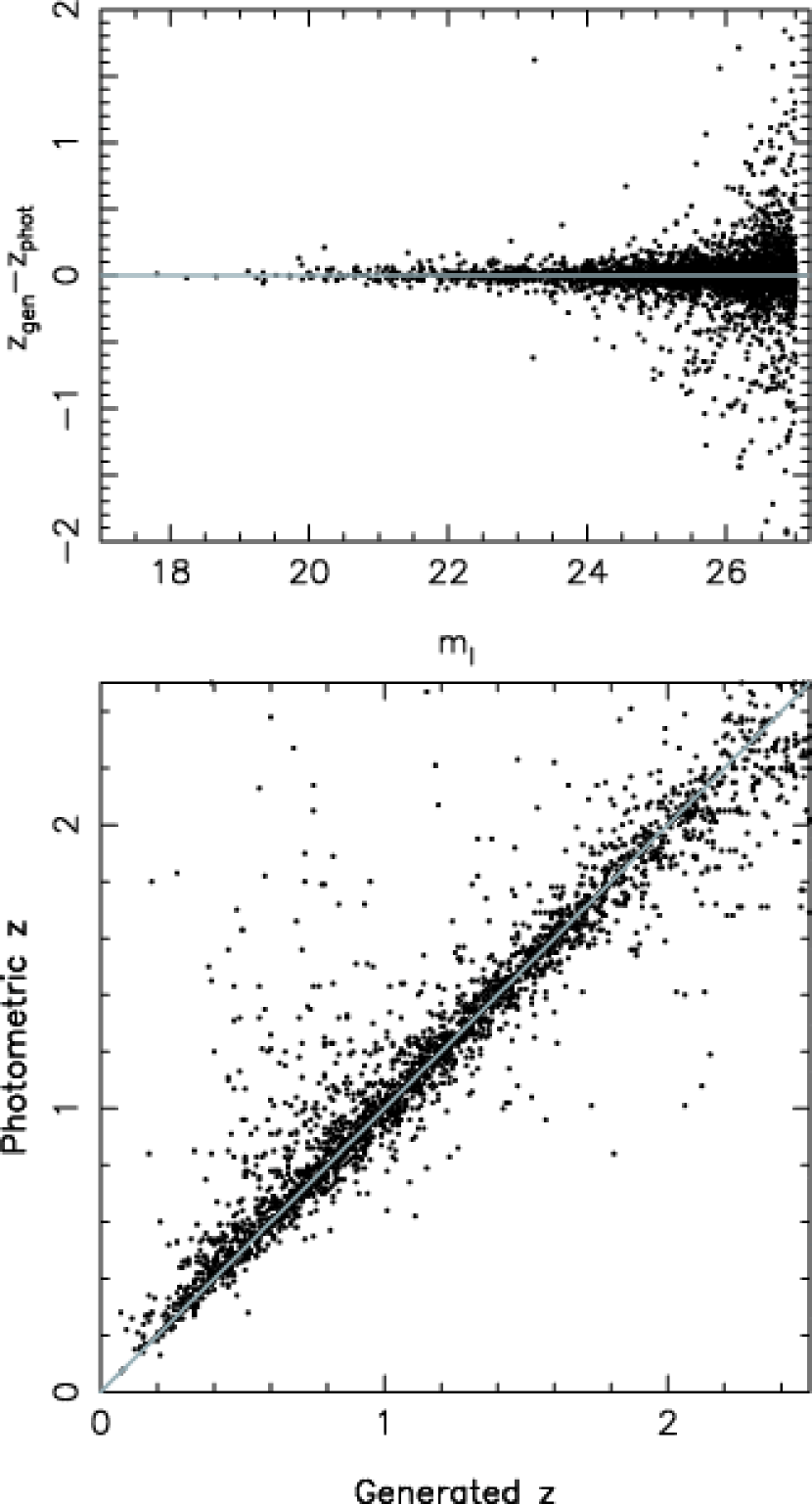
Figure 1 shows the simulated accuracy of the photometric redshifts for a survey with limiting magnitude $I<27$ (S/N=10). The bottom panel shows the generated (input) redshifts vs. the photometric redshifts, while the top panel shows the difference between generated and photometric redshifts as a function of galaxy magnitude.

4.1 Understanding the Magnification Uncertainties

We have identified and addressed the following uncertainties when estimating the lensing magnification of a specific source given a galaxy catalog:

• Finite field size

• The intrinsic scatter in, and accuracy of, the F–J and T–F relations

• Redshift and position uncertainties

• Choice of halo profile

• The magnitude limit

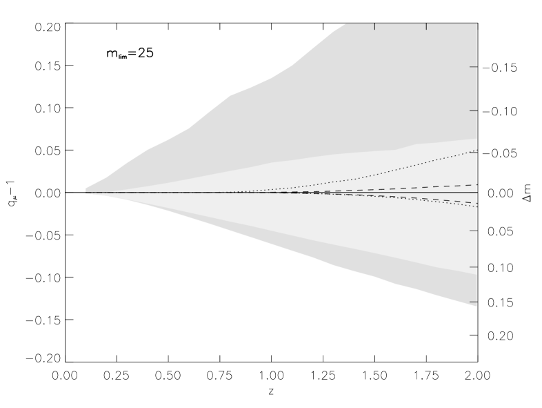
These sources of error are addressed individually in the following sections. Our reference model consists of NFW halos truncated at $r_{\rm t}=r_{\rm 200}$, velocity dispersion/circular velocity normalizations of 220 km  s^-1 for ellipticals, 203 km  s^-1 for spirals and source redshift $z=1.5$. In Figure 2, the Probability Distribution Function (PDF) for lensing magnifications for the reference model is shown. The lensing dispersion at $z=1.5$ is $\sim 7\,\%$. We analyze the results by comparing the distribution of magnifications in the reference model with the distribution obtained after performing a correction with the above-mentioned uncertainties. We denote the uncorrected value $\mu_{\rm ref}$ and the corrected one $q_{\mu}$, where

$$q_{\mu}=\frac{\mu_{\rm ref}}{\mu_{\rm est}},$$ (25)

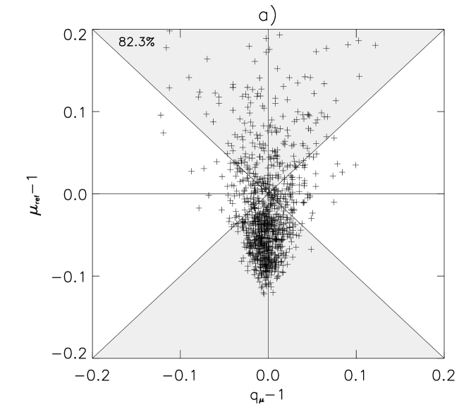
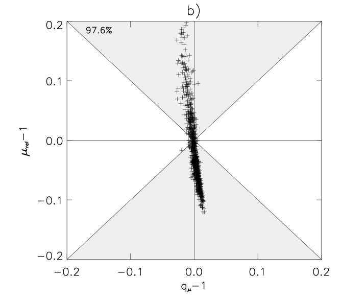
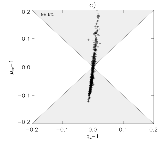
where $\mu_{\rm est}$ is the estimated magnification factor including one or more uncertainties. Corrections will reduce the uncertainties from lensing whenever the width of the distribution of $q_{\mu}$ is smaller than the corresponding width in the $\mu_{\rm ref}$ distribution. If no uncertainties were present $\mu_{\rm est}=\mu_{\rm ref}$ and $q_{\mu}=1$ implying a perfect correction. As a measure of the width we give the standard deviation of the distribution. Since many of the distributions are non-Gaussian, we also report the 68 % and 95 % confidence levels.

4.2 Finite Field Size

The mean magnification relative to an homogeneous universe of a large number of sources lensed by randomly distributed matter is expected to be unity due to photon number conservation. When we model a lensing system, only galaxies within angular radius $\theta_{\rm s}$ of the position of the source on the sky are taken into account and thus $\bar{\mu}<1$. If $\theta_{\rm s}$ is increased, more lenses are added and the mean magnification increases. This dependence is illustrated in Figure 3, showing the mean magnification of 5000 point sources, as a function of $\theta_{\rm s}$. The mean magnification increases rapidly for small $\theta_{\rm s}$, but only slowly for $\theta_{\rm s}$ larger than an arc-minute, where the error is $\sim 1\,\%$. In our simulations, we use $60^{\prime\prime}$ as a cutoff to save computing time. In a real survey, a cutoff will have to be introduced for practical purposes since only a limited portion of the sky will be observed. In order to avoid a systematic bias due to the finite field size for a given survey, the computed magnifications should be corrected with a factor corresponding to the inverse of the mean magnification for the cutoff radius used. In the following, we have neglected this small ($\sim 1\,\,\%$) correction. Furthermore, going to larger $\theta_{\rm s}$ would not render $\bar{\mu}$ being exactly unity since some flux is lost whenever multiple imaging occurs. Q-LET gives the magnification and intrinsic source position of a given image, not observed position and magnification of a given source. Therefore, in the rare cases of multiple imaging, only one of the images will be taken into account resulting in some flux loss. Note also that since random l-o-s and random source positions are different (e.g., Schneider, Ehlers & Falco, 1992), we have to use a magnification dependent weighting procedure to see whether each simulated event should be kept or discarded in order to get a sample of random source positions (see e.g., Goobar et al., 2002).

4.3 The F–J and T–F Relations

The F–J and T–F relations give the velocity dispersions of the luminous matter and we make the assumption that the dark matter that constitutes the halo follows scales in the same way. Both the Faber-Jackson and the Tully-Fisher relations have an intrinsic scatter with an rms estimated in §3.3. To study the effect of this scatter, we add random offsets to the F–J and T–F relations when calculating the halo mass. Since we do not want to bias the total mass in our simulations, we distribute the offsets using a Gaussian distribution in $\sigma^{3}$ (since mass $\propto\sigma^{3}$). We derive the width of the Gaussian (one sigma value in $\sigma^{3}$) from the rms in log${}_{10}(\sigma)$ and log${}_{10}(V_{\rm max})$ using Eqs. (11)-(12) (F–J) and Eqs. (13)-(15) (T–F).

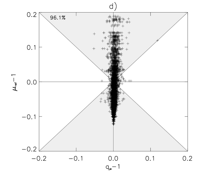
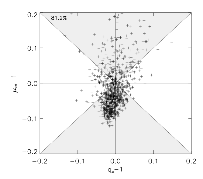
In panel a) in Figure 4, we compare the distribution of the corrected value $q_{\mu}$ due to the scatter in the F–J and T–F relations with the distribution of magnifications in the reference model (dashed line). Note that if we knew all velocity dispersions and circular velocities exactly, $q_{\mu}$ would be represented by a $\delta$-function at $q_{\mu}=1$. We see that the intrinsic scatter in the velocity dispersion and circular velocity causes a dispersion of $q_{\mu}$ of approximately $3\,\%$, a factor of $\sim 2.6$ less than the original dispersion. Panel a) in Figure 5 shows $\mu_{\rm ref}-1$ vs $q_{\mu}-1$ for each individual source. For $82\,\%$ of the sources, the corrected luminosity will be better than the uncorrected one.

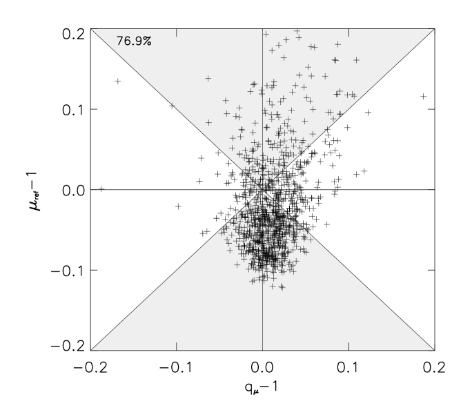
Besides the intrinsic scatter in the F–J and T–F relations, there is also a possible systematic uncertainty in $\sigma_{*}$. To estimate this, we use SDSS data in Bernardi et al. (2003) where photometric and spectroscopic parameters for a sample of $\sim 9000$ early-type galaxies in the redshift range $0.01<z<0.3$ are given, including K-corrections and accurately measured velocity dispersions. We fit a straight line $M_{B}=b\log\sigma+a$ and estimate the error in $\sigma_{*}$ for a given $M_{B}^{*}$ by propagating the errors in the parameters $a$ and $b$. For $M_{B}^{*}=-21.04$, we obtain $\sigma_{*}=218\pm 7$ km  s^-1. In panel b) and c) in Figure 4, we investigate the effect of a systematic shift of $\pm 10$ km  s^-1 in $\sigma_{*}$. The dispersion in $q_{\mu}$ due to such a shift is quite small or at the order of $1\,\%$. Panels b) and c) in Figure 5 shows $\mu_{\rm ref}-1$ vs $q_{\mu}-1$ for each individual source. The corrected value will be better than the uncorrected for $>95\,\%$ of the sources.

A further source that may increase the scatter in the magnification is the possible misclassification of galaxy morphology. An elliptical galaxy wrongly classified as a spiral, leads to an underestimation of the underlying mass, and vice versa if a spiral is misclassified as an elliptical. To investigate the possible effect of this, we first use a set of simulated galaxies with known morphological types (i.e. an exponential radial profile for spirals and a de Vaucouleurs profile for ellipticals) and measure how many are correctly recovered in an observational setup resembling the GOODS. To classify galaxies, we use the GALFIT software (Peng et al., 2002), which measures the slope of the radial profile and therefore allows a discrimination between ellipticals and spirals. At a S/N=10 detection limit (m$\sim$25), we find that $\sim$25 % of the ellipticals and $\sim$8 % of the spirals are misclassified. The fraction of misclassified galaxies quickly drops to $\sim$1 % at a magnitude $\sim$2 mag brighter than the detection limit. We then use these results to estimate the effect of misclassification on the derived magnifications. We find that the increase in the scatter in the magnification is $\sim$0.5 % due to this effect. Therefore, misidentification of galaxy morphology should only affect the results marginally. However, for ground-based surveys with low resolution, the effect may be larger.

4.4 Redshift and Position Uncertainties

Uncertainties in the redshifts of the lenses will alter the results both through the uncertain distances between different lens-planes and by introducing an uncertainty in their absolute magnitudes used in the F–J and T–F relations.

In an ideal observational situation, all redshifts are determined spectroscopically. In many real situations, however, only photometric redshift are available due to, e.g., the faintness of the galaxies and the large number of sources. To investigate the effects of photometric redshift uncertainties, we add a random offset to the redshift of each object. The size of the offset depends on redshift, apparent magnitude and spectral type of the object and is drawn from the simulated error distribution discussed above.

In panel d) in Figure 4, we show the distribution of the corrected value $q_{\mu}$ due to a random offset to the redshift of each lensing object. The induced error in the estimated magnification is less than $1\,\%$. The corresponding panel in Figure 5 shows $\mu_{\rm ref}-1$ vs $q_{\mu}-1$ for each individual source. In this case, $96\,\%$ of the sources have corrected values which are better than when uncorrected.

Besides the Gaussian-like distribution of the photometric redshift errors investigated above, there is also a possibility that a fraction of the objects get ”catastrophic redshifts” with large errors, so called outliers. E.g., by comparing with $\sim$1400 spectroscopic redshifts in the CDF-S and HDF-N, we find that the GOODS photometric redshifts have about 3 % outliers with $\Delta_{z}>0.3$. The redshift probability distribution, for a majority of these objects are characterized by a primary ($\sim$Gaussian) peak combined with a less pronounced secondary peak. Outliers are foremost objects assigned the redshift of the primary peak, but where the true redshift is that of the secondary peak. To estimate the effect of outliers, we use the galaxies in the GOODS and simulate the case where we distribute the photometric redshifts over the full probability distribution, including the secondary peak. This will allow $\sim$3 % outliers. We compare this with the case where we only include redshifts in the primary peak (i.e. objects with $\Delta_{z}<0.3$). We find that the increase in lensing dispersion due to the population of outliers is less than 1 %. One reason for the small effect is that outliers are mainly faint and very blue objects, which therefore should have relatively small masses.

Any error in the exact positions of the lensing galaxies can also affect the resulting magnification. Apart from the observational error, such an effect can be due to a misalignment between the luminous and the dark matter in a given galaxy. We have investigated the effect of a Gaussian random shift with $\sigma_{\rm pos}=0.5$ arcseconds of all lensing galaxies along the l-o-s. Even such a large shift of all galaxy positions results in a distribution of corrected values $q_{\mu}$ with a dispersion of less than $0.5\,\%$.

4.5 Choice of Halo Profile

The choice of halo model is only important in those lens-planes where the light-ray passes through a halo. If passing outside, the halo will act as a point mass and when $m_{\rm tot}^{\rm halo}=m_{200}^{\rm SIS}=m_{200}^{\rm NFW}$ the two different halo models give exactly the same results.

We have performed simulations where all halos were of SIS instead of NFW type. The effect of different halo profiles are also present in the realistic and pessimistic case simulations below.

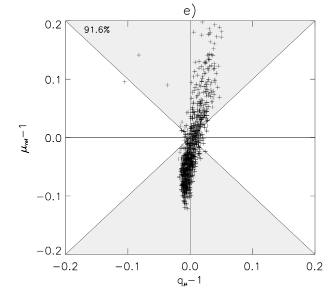
Panel e) in Figure 4 shows the PDF of $q_{\mu}$ when assuming SIS halos instead of NFW as in the reference model. The dispersion is less than $1.5\,\%$. In $>90\,\%$ of the cases, the corrected value is better than the uncorrected, see panel e) in Figure 5.

We have also investigated how important the assumption on the truncation radius is for the resulting magnification distribution by running tests with $0.75\times r_{200}\leq r_{\rm t}\leq 1.25\times r_{200}$ for the SIS model. The uncertainty in the resulting magnification gives a distribution of corrected values $q_{\mu}$ with a dispersion of $\sim 0.5-1\,\%$. Since the NFW profile falls of as $\rho_{\rm NFW}\propto r^{-3}$ at large radii as compared to $\rho_{\rm SIS}\propto r^{-2}$ for SIS halos, this should be considered a very conservative limit on the effect of changing the truncation radius.

4.6 Magnitude Limits

Our reference model uses a constant comoving mass density of galaxies, implying a constant smoothness parameter, $\eta$. In a real scenario with an observational magnitude limit, an increasing fraction of galaxies drop out at higher redshift. The faint high redshift galaxies will not be seen and hence not included as lenses in the magnification calculation but instead added as homogeneously distributed matter. Therefore, when deriving the smoothness parameter from observations, $\eta(z)$ increases with redshift even if the ’underlying’ smoothness parameter is constant. For each simulation with a finite magnitude limit, a new $\eta$-function is computed using the method described in §3.2.

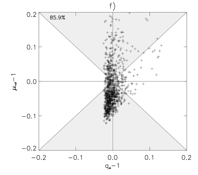
For $I=27$ mag the distribution of $q_{\mu}$ is very narrow and for $I=29$ mag, it is in principle a $\delta$-function. Panel f) in Figure 4 shows the PDF of $q_{\mu}$ for $I=23$. The dispersion is $\sim 2\,\%$. In $86\,\%$ of the cases, the corrected value is better than the uncorrected, see panel f) in Figure 5.

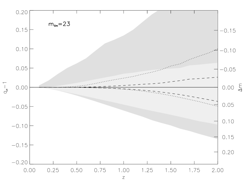
In Figure 6, we compare $q_{\mu}-1$ as a function of source redshift for models with magnitude limits $I=23$ and $I=25$ with $\mu_{\rm ref}-1$. Even for source redshifts as high as $z\sim 2$, a magnitude limit of $I=23$ does not significantly impair our results.

Photometric errors in the apparent magnitudes translates to an increased scatter in the absolute magnitudes and therefore also in the derived velocity dispersions and masses. At the faintest magnitude limits considered here, S/N=10, typical errors are $\sim 0.1$ mag. For ellipticals, this corresponds to an increased dispersion of $\Delta{\rm log_{10}}\sigma\sim 0.01$ (using Eq. 10). This is significantly less than the intrinsic scatter in the F–J relation which is rms(log${}_{10})\sigma\sim 0.08$ (at $\sim M_{B}^{*}$, Eq. 12). For the T–F relation the increased scatter due to photometric errors is $\Delta{\rm log_{10}}V_{\rm max}\sim 0.013$ (using Eq. 13), again significantly less than the intrinsic scatter rms(log${}_{10}V_{\rm max})\sim 0.06$. So even for the faintest galaxies considered, the errors in apparent magnitude should not affect results more than marginally.

4.7 Realistic and Pessimistic Scenarios

We have studied the uncertainty in the lensing correction in a realistic scenario where a reasonable error budget is assumed. In this case we have assumed 50 % NFW, 50 % SIS, no central value shift of the velocity dispersion normalization but a dispersion around this value and a magnitude limit of $I=25$. Lens redshifts were assumed to be distributed around their reference values. As the correct model we have used the reference NFW model as above.

A pessimistic scenario for space based surveys has also been studied where we have maximized the uncertainties in relating the luminous and the dark matter. However, one could easily imagine worse cases in a ground-based experiment. For our scenario the erroneous assumptions were: SIS halos, central value of velocity dispersion normalization shifted +10 km  s^-1 and distributed around this value, a magnitude limit of $I=25$, lens redshifts assumed to be distributed around their reference model values, an offset in lens positions as described in §4.4 and finally a truncation radius of $1.25\times r_{200}$. We consider this being a pessimistic but not completely unrealistic scenario.

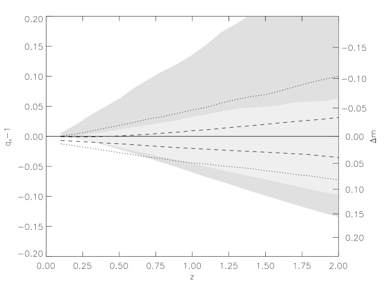
The left panels in Figure 7 show results for the realistic scenario, the right panels for the pessimistic scenario. For the realistic case, $q_{\mu}$ has a dispersion of $\sim 3\,\%$ and $(q_{\mu}-1)<(\mu_{\rm ref}-1)$ for $\sim 80\,\%$ of the sources. In the pessimistic case, the corresponding numbers are $\sim 3\,\%$ and $\sim 77\,\%$, i.e. our ability to correct for lensing is more or less unimpaired when going from a realistic to a pessimistic scenario. The bottom row shows $q_{\mu}-1$ as a function of source redshift for the two scenarios. The confidence levels of the realistic case vs $z$ can be well fitted with straight lines and these are found in Table 1 expressed in magnitudes.

5 SUMMARY AND DISCUSSION

We have investigated the accuracy to which lensing magnification can be estimated on individual lines of sight using the observed properties of the foreground galaxies of each source.

The result depends on the uncertainties in translating observed galaxy luminosities to the (invisible) matter distribution in the lensing galaxies. We have shown that none of the studied uncertainties neither individually nor combined will render the corrected distribution of magnifications wider than the dispersion from lensing. Even for a pessimistic scenario, the dispersion due to lensing for a standard candle source at $z=1.5$ can be reduced by a factor $\gtrsim 2$, comparable to the result for a realistic scenario. The reason our pessimistic case result is not significantly worse than for the realistic case, is that the uncertainties are dominated by the scatter in the F–J and T–F relations for both scenarios. At lower redshifts ($z\lesssim 0.5$), the effects from lensing are small and correcting for lensing is not likely to improve the results.

Even though the fraction of SNe lines-of-sight passing through galaxy cluster lenses is expected to be relatively low, these are potentially important due to magnification bias and in surveys specifically aimed at using cluster potentials as gravitational telescopes (Gunnarsson & Goobar, 2003). In those cases, individual modeling of the cluster potentials using, e.g., weak and strong lensing of background galaxies is needed to correct the observed magnitudes for the lensing magnification. Alternatively, one can choose to discard SNe background to galaxy clusters with very uncertain matter distributions when estimating cosmological parameters.

Our method also takes into account gravitational lensing from large scale dark matter structures such as filaments and walls as long as the matter density is dominated by the individual galaxy size halos. If we very conservatively assume that large scale structures are completely uncorrelated with the luminous matter, we expect the lensing magnification contribution to be less than 2 % on scales larger than 5 arcminutes (for a source redshift of unity) (Cooray et al., 2005).

For a given galaxy catalog, the computed magnifications do not depend strongly on the cosmological parameters used. However, since the formation of matter structure is a function of cosmology, it should in principle be possible to determine the cosmology from the observed distribution of standard candle luminosities. In this case, the use of magnifications of e.g. SNIa would be similar to using shear of background galaxies as in weak lensing studies. Such a study would require large statistics of very well observed SNIa and will probably have to await future dedicated missions such as the proposed SNAP satellite .

For current high-$z$ SNIa observations the concern is to correct for the magnification and investigate the possibility for magnification bias. Such a study for SNe in the GOODS fields is described in a accompanying paper (Jönsson et al., 2005) where magnification bias is shown to be negligible but lensing for individual SNe can be estimated quite robustly from foreground galaxy observations and thus be corrected for. In fact, as long as the luminous and dark matter are not anti-correlated, we would expect to be able to reduce the scatter in the Hubble diagram by assuming that dark matter follows light. Thus, we find that even though the exact relation between luminous and dark matter is uncertain, correcting for gravitational lensing using observed galaxy properties should be harmless at the worst and very useful at the best.

The authors would like to thank Mariangela Bernardi for help with the velocity dispersion data from the Sloan survey, Joakim Edsjö, Daniel Holz and Saul Perlmutter for helpful discussions during the course of the work. We are grateful to Swara Ravindranath for providing simulated galaxy catalogs used to derive the recovery fraction of galaxy morphologies. CG would like to thank the Swedish Research Council for financial support. AG is a Royal Swedish Academy Research Fellow supported by grants from the Swedish Research Council, the Knut and Alice Wallenberg Foundation and the Göran Gustafsson Foundation for Research in Natural Sciences and Medicine.

Equation: $y=kz+m$
	Uncorrected		Corrected
	$k$	$m$	$k$	$m$
68 % magn.	-0.038	0.005	-0.020	0.008
68 % demagn.	0.060	-0.009	0.016	0.006
95 % magn.	-0.140	-0.003	-0.055	0.008
95 % demagn.	0.086	-0.017	0.035	0.012

Table 1: Fits to the confidence levels of Fig. 7 expressed in magnitudes. Note that these are only valid for $z\gtrsim 0.25$. However, below this value the corrections are indeed very small.

Figure 1: Bottom panel shows generated (input) redshifts vs. derived photometric redshifts for a simulated survey with limiting magnitude $I<27$ (S/N=10). Top panel shows the difference between generated and photometric redshifts as a function of observed galaxy magnitude.

Figure 2: PDF of magnifications for the reference model with NFW halos truncated at $r_{\rm t}=r_{\rm 200}$, no magnitude limit, velocity dispersion/circular velocity normalizations 220 km  s^-1 for ellipticals, 203 km  s^-1 for spirals, no uncertainty in halo redshifts and source redshift $z=1.5$

Figure 3: Mean magnification $\bar{\mu}$ of 5000 lines-of-sight as a function of $\theta_{\rm s}$. The sources all have redshifts $z=1.5$.

Figure 4: PDFs of $q_{\mu}$ where the following uncertainties have been studied: a) The scatter in the velocity dispersion of the F–J and T–F relations, b) Offset in central value of $\sigma_{*}$ of $+10$ km  s^-1, c) Offset in central value of $\sigma_{*}$ of $-10$ km  s^-1, d) Lens redshifts distributed around their original values, e) Assuming SIS halos instead of NFW and f) Assuming a magnitude limit of $I=23$ mag. The PDF before correction (dashed line) is also plotted for reference.

Figure 5: Spread in $\mu_{\rm ref}-1$ vs spread in $q_{\mu}-1$ where the following uncertainties have been studied: a) The scatter in the velocity dispersion of the F–J and T–F relations, b) Offset in central value of $\sigma_{*}$ of $+10$ km  s^-1, c) Offset in central value of $\sigma_{*}$ of $-10$ km  s^-1, d) Lens redshifts distributed around their original values, e) Assuming SIS halos instead of NFW and f) Assuming a magnitude limit of $I=23$ mag. The gray shaded areas show where the value after correction is closer to reality than before correction. The figures in the upper left corners give the percentage of events residing in the gray areas, where the correction improves the resulting accuracy of the derived distance.

Figure 6: $q_{\mu}-1$ as a function of source redshift for a models with magnitude limits $I=23$ and $I=25$, using 1700 lines-of-sight for each redshift. The gray shaded areas show the 68 % and 95 % confidence levels of $\mu_{\rm ref}-1$, the distance from the correct value 1 before correction. The dashed and dotted lines show the same confidence levels after correction clearly indicating the improvement.

Figure 7: Left column shows a realistic scenario with 50 % NFW, 50 % SIS, values of velocity dispersion distributed around their central value, lens redshift values distributed around their reference model values and finally using a magnitude limit of $I=25$ mag. The right column shows a pessimistic scenario with with 100 % SIS, values of velocity dispersion normalization distributed around a +10 km  s^-1 shifted central value, a small random offset $(\sigma_{\rm pos}=0.5^{\prime\prime})$ in lens positions, truncation radius of $1.25\times r_{200}$ and the rest as in the realistic case. The upper row gives the PDFs and confidence levels for sources at redshift $z=1.5$, middle row shows the spread in $\mu_{\rm ref}-1$ vs the spread in $q_{\mu}-1$. The bottom row shows confidence levels of the two scenarios vs source redshift.

References

- Amanullah, Mörtsell & Goobar (2003) Amanullah, R., Mörtsell, E., Goobar, A., 2003, A&A, 397, 819
- Benítez et al. (2002) Benítez, N., Riess, A. G., Nugent, P. E., Dickinson, M., Chornock, R., Filippenko, A. V., ApJ, 577, L1
- Bernardi et al. (2003) Bernardi, M., et al., 2003, AJ, 125, 1817
- Böhm et al. (2004) Böhm, A., et al., 2004, A&A, 420, 97
- Cooray et al. (2005) Cooray, A., Huterer, D., & Holz, D., 2005, astro-ph/0509581
- Dahlén et al. (2005) Dahlén T., Mobasher, B., Somerville, R., Moustakas, L., Dickinson, M., Ferguson, H., Giavalisco, M., 2005, ApJ, 631, 126
- Goobar & Perlmutter (1995) Goobar, A., Perlmutter. S, 1995, ApJ, 450, 14
- Goobar et al. (2002) Goobar, A., Mörtsell, E., Amanullah, R., Goliath, M., Bergström, L., Dahlén, T., 2002, A&A, 392, 757
- Gunnarsson (2004) Gunnarsson, C., 2004, JCAP, 0403, 002
- Gunnarsson & Goobar (2003) Gunnarsson, C., & Goobar, A. 2003, A&A, 405, 859
- Holz & Linder (2004) Holz, D., Linder, E., 2005, ApJ, 631, 678
- Holz & Hughes (2005) Holz, D., Hughes, S. A., 2005, ApJ, 629, 15
- Jönsson et al. (2005) Jönsson, J., Dahlén, T., Goobar, A, Gunnarsson, C., Mörtsell, E., 2005, submitted to ApJ
- Kayser et al. (1997) Kayser, R., Helbig, P., Schramm, T., 1997, A&A, 318, 680
- Knop et al. (2003) Knop, R., et al., 2003, ApJ, 598, 102
- Lewis & Ibata (2001) Lewis, G. F., Ibata, R. A., 2001, MNRAS, 324, L25
- Mitchell et al. (2005) Mitchell, J., Keeton, C.,Frieman, J., Sheth, R., 2005, ApJ, 622, 81
- Mörtsell, Gunnarsson & Goobar (2001) Mörtsell, E, Gunnarsson, C., Goobar, A., 2001, ApJ, 561, 106; erratum ibid 2003, 589, 1089
- Navarro, Frenk & White (1997) Navarro, J. F., Frenk, C. S., White, S. D. M., 1997, ApJ, 490, 93
- Peng et al. (2002) Peng, C.Y., Ho, L.C., Impey, C.D., & Rix, H.-W. 2002, AJ, 124, 266
- Perlmutter et al. (1998) Perlmutter, S., et al., 1998, Nature, 391, 51
- Perlmutter et al. (1999) Perlmutter, S., et al., 1999, ApJ, 517, 565
- Pierce & Tully (1992) Pierce, M. J., Tully, R. B., ApJ, 387, 47
- Riess et al. (1998) Riess, A. G., et al., 1998, AJ, 116, 1009
- Riess et al. (2004) Riess, A. G., et al., 2004, ApJ, 607, 665
- Schmidt et al. (1998) Schmidt, B. P., et al., 1998, ApJ, 507, 46
- Schneider, Ehlers & Falco (1992) Schneider, P., Ehlers, J., Falco, E. E., 1992, Gravitational Lenses, Springer-Verlag, Berlin
- Sheth et al. (2003) Sheth, R. K., et al., 2003, ApJ, 594, 225
- Strolger et al. (2004) Strolger, L.-G., et al., 2004, ApJ, 613, 200
- Tonry et al. (2003) Tonry, J. L., et al., 2003, ApJ, 594, 1