Spectral analysis of early-type stars using a
genetic algorithm based fitting method

We present the first automated fitting method for the quantitative spectroscopy of O- and early B-type stars with stellar winds. The method combines the non-LTE stellar atmosphere code fastwind from Puls et al. (2005) with the genetic algorithm based optimizing routine pikaia from Charbonneau (1995), allowing for a homogeneous analysis of upcoming large samples of early-type stars (e.g. Evans et al. 2005). In this first implementation we use continuum normalized optical hydrogen and helium lines to determine photospheric and wind parameters. We have assigned weights to these lines accounting for line blends with species not taken into account, lacking physics, and/or possible or potential problems in the model atmosphere code. We find the method to be robust, fast, and accurate. Using our method we analysed seven O-type stars in the young cluster Cyg OB2 and five other Galactic stars with high rotational velocities and/or low mass loss rates (including 10 Lac, $\zeta$ Oph, and $\tau$ Sco) that have been studied in detail with a previous version of fastwind. The fits are found to have a quality that is comparable or even better than produced by the classical “by eye” method. We define errorbars on the model parameters based on the maximum variations of these parameters in the models that cluster around the global optimum. Using this concept, for the investigated dataset we are able to recover mass-loss rates down to $\sim$ $6\times 10^{-8}\mbox{$M_{\sun}{\rm yr}^{-1}$}$ to within an error of a factor of two, ignoring possible systematic errors due to uncertainties in the continuum normalization. Comparison of our derived spectroscopic masses with those derived from stellar evolutionary models are in very good agreement, i.e. based on the limited sample that we have studied we do not find indications for a mass discrepancy. For three stars we find significantly higher surface gravities than previously reported. We identify this to be due to differences in the weighting of Balmer line wings between our automated method and “by eye” fitting and/or an improved multidimensional optimization of the parameters. The empirical modified wind momentum relation constructed on the basis of the stars analysed here agrees to within the error bars with the theoretical relation predicted by Vink et al. (2000), including those cases for which the winds are weak (i.e. less than a few times $10^{-7}$ $M_{\sun}{\rm yr}^{-1}$).

1 Introduction

Until about a decade ago detailed analysis of the photospheric and wind properties of O-type stars was limited to about 40 to 50 stars divided over the Galaxy and the Magellanic Clouds (see e.g. Puls et al. 1996; see also Repolust, Puls, & Herrero 2004). The reason that at that time only such a limited number of objects had been investigated is related in part to the fact that considerable effort was directed towards improving the physics of the non-local thermodynamic equilibrium (non-LTE) model atmospheres used to analyse massive stars. Notable developments have been the improvements in the atomic models (e.g. Becker & Butler 1992), shock treatment (Pauldrach et al. 2001), clumping (Hillier 1991; Hillier & Miller 1999), and the implementation of line blanketing (e.g. Hubeny & Lanz 1995; Hillier & Miller 1998; Pauldrach et al. 2001). To study the effects of these new physics a core sample of “standard” O-type stars has been repeatedly re-analysed. A second reason, that is at least as important, is the complex, and time and CPU intensive nature of these quantitative spectroscopic analyses. Typically, at least a six dimensional parameter space has to be probed, i.e. effective temperature, surface gravity, helium to hydrogen ratio, atmospheric microturbulent velocity, mass-loss rate, and a measure of the acceleration of the transonic outflow. Rotational velocities and terminal outflow velocities can be determined to considerable accuracy by means of external methods such as rotational (de-) convolution methods (e.g. Howarth et al. 1997) and SEI-fitting of P-Cygni lines (e.g. Groenewegen & Lamers 1989), respectively. To get a good spectral fit it typically requires tens, sometimes hundreds of models per individual star.

In the last few years the field of massive stars has seen the fortunate development that the number of O-type stars that have been studied spectroscopically has been doubled (e.g. Crowther et al. 2002; Herrero et al. 2002; Bianchi & Garcia 2002; Bouret et al. 2003; Hillier et al. 2003; Garcia & Bianchi 2004; Martins et al. 2004; Massey et al. 2004; Evans et al. 2004). The available data set of massive O- and early B-type stars has recently again been doubled, mainly through the advent of multi-object spectroscopy. Here we explicitly mention the VLT-FLAMES Survey of Massive Stars (Evans et al. 2005) comprising over 100 hours of VLT time. In this survey multi-object spectroscopy using the Fibre Large Array Multi-Element Spectrograph (FLAMES) has been used to secure over 550 spectra (of which in excess of 50 are spectral type O) in a total of seven clusters distributed over the Galaxy and the Magellanic Clouds.

This brings within reach different types of studies that so far could only be attempted with a troublingly small sample of stars. These studies include establishing the mass loss behaviour of Galactic stars across the upper Hertzsprung-Russell diagram, from the weak winds of the late O-type dwarfs (of order $10^{-8}$ $M_{\sun}{\rm yr}^{-1}$) to the very strong winds of early O-type supergiants (of order $10^{-5}$ $M_{\sun}{\rm yr}^{-1}$); determination of the mass-loss versus metallicity dependence in the abundance range spanned by Small Magellanic Cloud to Galactic stars; placing constraints on the theory of massive star evolution by comparing spectroscopic mass determinations and abundance patterns with those predicted by stellar evolution computations, and the study of (projected) spatial gradients in the mass function of O- and B-type stars in young clusters, as well as such spatial gradients in the initial atmospheric composition of these stars.

To best perform studies such as listed above not only requires a large set of young massive stars, it also calls for a robust, homogeneous and objective means to analyse such datasets using models that include state-of-the-art physics. This essentially requires an automated fitting method. Such an automated method should not only be fast, it must also be sufficiently flexible to be able to treat early-type stars with widely different properties (e.g. mass-loss rates that differ by a factor of $10^{3}$). Moreover, it should apply a well defined fitting criterium, like a $\chi^{2}$ criterium, allowing it to work in an automated and reproducible way.

To cope with the dataset provided by the VLT-FLAMES Survey and to improve the objectivity of the analysis, we have investigated the possibility of automated fitting. Here we present a robust, fast, and accurate method to perform automated fitting of the continuum normalized spectra of O- and early B-type stars with stellar winds using the fast performance stellar atmosphere code fastwind (Puls et al. 2005) combined with a genetic algorithm based fitting method. This first implementation of an automated method should therefore be seen as an improvement over the standard “by eye” method, and not as a replacement of this method. The improvement lies in the fact that with the automated method large data sets (tens or more stars), spanning a wide parameter space, can be analysed in a repeatable and homogeneous way. It does not replace the “by eye” method as our automated fitting method still requires a by eye continuum normalization as well as a human controlled line selection. This latter should address the identification and exclusion of lines that are not modeled (i.e. blends), as well as introduce information on lacking physics and/or possible or potential problems in the model atmosphere code. Future implementations of an automated fitting method may use the absolute spectrum, preferably over a broad wavelength range. This would eliminate the continuum rectification problem, however, it will require a modeling of the interstellar extinction. In this way one can work towards a true replacing of the “by eye” method by an automated approach.

In Sect. 2 we describe the genetic algorithm method and implementation, and we provide a short résumé of the applied unified, non-LTE, line-blanketed atmosphere code fastwind – which is the only code to date for which the method described here is actually achievable (in the context of analysing large data sets). To test the method we analyse a set of 12 early type spectra in Sect. 3. We start with a re-analysis of a set of seven stars in the open cluster Cyg OB2 that have been studied by Herrero et al. (2002). The advantage of focusing on this cluster is that it has been analysed with a previous version of fastwind, allowing for as meaningful a comparison as is possible, while still satisfying our preference to present a state-of-the-art analysis. The analysis of Cyg OB2 has the added advantage that all stars studied are approximately equidistant. To test the performance of our method outside the parameter range offered by the Cyg OB2 sample we have included an additional five well-studied stars with either low density winds and/or very high rotational velocities. In Sect. 4 we describe our error analysis method for the multidimensional spectral fits obtained with the automated method. A systematic comparison of the obtained parameters with previously determined values is given in Sect. 5. Implications of the newly obtained parameters on the properties of massive stars are discussed in Sect. 6. In the last section we give our conclusions.

2 Automated fitting using a genetic algorithm

2.1 Spectral line fitting as an optimization problem

Spectral line fitting of early-type stars is an optimization problem in the sense that one tries to maximize the correspondence between a given observed spectrum and a synthetic spectrum produced by a stellar atmosphere model. Formally speaking one searches for the global optimum, i.e. best fit, in the parameter space spanned by the free parameters of the stellar atmosphere model by minimizing the differences between the observed and synthesized line profiles.

Until now the preferred method to achieve this minimization has been the so called fitting “by eye” method. In this method the best fit to the observed spectrum of a certain object is determined in an iterative manner. Starting with a first guess for the model parameters a spectrum is synthesized. The quality of the fit to the observed spectrum is determined, as is obvious from the methods name, by an inspection by eye. Based on what the person performing the fit sees, for instance, whether the width of the line profiles are reproduced correctly, combined with his/her experience and knowledge of the model and the object, the model parameters are modified and a new spectrum is synthesized. This procedure is repeated until the quality of the fit determined by eye cannot be increased anymore by modifying the model parameters.

It can be questioned whether a fit constructed with the fitting “by eye” method corresponds to the best fit possible, i.e. the global optimum. Reasons for this are, i) the restricted size of parameter space that can be investigated, both in terms of number of free parameters as well as absolute size of the parameter domain that can investigated with high accuracy, ii) the limited number of free parameters that are changed simultaneously, and iii) biases introduced by judging the quality of a line fit by eye. The importance of the first point lies in the fact that in order to assure that the global optimum is found, a parameter space that is as large as possible should be explored with the same accuracy for all parameters in the complete parameter space. If this is not the case the solution found will likely correspond to a local optimum.

The argument above becomes stronger in view of the second point. Spectral fitting is a multidimensional problem in which the line profile shapes depend on all free parameters simultaneously, though to a different extent. Consequently, the global optimum can only be found if all parameters are allowed to vary at the same time. The use of fit diagrams (e.g. Kudritzki & Simon 1978; Herrero et al. 1992) does not resolve this issue. These diagrams usually only take variations in $T_{\rm eff}$ and $\log{{g}}$ into account, neglecting the effects of other parameters, like microturbulence (e.g. Smith & Howarth 1998; Villamariz & Herrero 2000) and mass loss (e.g. [Fig. 5 of] Mokiem et al. 2004), on the line profiles.

The last point implies that, strictly speaking, fitting “by eye” cannot work in a reproducible way. There is no uniform well defined method to judge how well a synthetic line profile fits the data by eye. More importantly, it implies that there is no guarantee that the synthetic line profiles selected by the eye, correspond to the profiles which match the data the best. This predominantly increases the uncertainty in the derivation of those parameters that very sensitively react to the line profile shape, like for instance the surface gravity.

The new fitting method presented here does not suffer from the drawbacks discussed above. It is an automated method capable of global optimization in a multi-dimensional parameter space of arbitrary size (Sect. 2.5). As it is automated, it does not require any human intervention in finding the best fit, avoiding potential biases introduced by “by eye” interpretations of line profiles. The method described here consists of two main components. The first component is the non-LTE stellar atmosphere code fastwind. Section 2.4 gives an overview of the capabilities of the code and the assumptions involved. The second component is the genetic algorithm (GA) based optimizing routine pikaia from Charbonneau (1995), which is responsible for optimizing the parameters of the fastwind models. For the technical details of this routine and more information on GAs we refer to the cited paper and references therein. Here we will suffice with a short description of GAs and a description of the GA implementation with respect to optimization of spectral fits.

2.2 The genetic algorithm implementation

Genetic algorithms represent a class of heuristic optimization techniques, which are inspired by the notion of evolution by means of natural selection (Darwin 1859). They provide a method of solving optimization problems by incorporating this biological notion in a numerical fashion. This is achieved by evolving the global solution over subsequent generations starting from a set of randomly guessed initial solutions, so called individuals. Selection pressure is imposed in between generations based on the quality of the solutions, their so called fitness. A higher fitness implies a higher probability the solution will be selected for reproduction. Consequently, only a selected set of individuals will pass on their “genetic material” to subsequent new generations.

To create the new generations discussed above GAs require a reproduction mechanism. In its most basic form this mechanism consists of two genetic operators. These are the crossover operator, simulating sexual reproduction, and the mutation operator, simulating copying errors and random effects affecting a gene in isolation. An important benefit of these two operators is the fact that they also introduce new genetic material into the population. This allows the GA to explore new regions of parameters space, which is important in view of the existence of local extremes. When the optimization runs into a local optimum, these two operators, where usually mutation has the strongest effect, allow for the construction of individuals outside of this optimum, thereby allowing it to find a path out of the local optimum. This capability to escape local extremes, consequently, classifies GAs as global optimizers and is one of the reasons they have been applied to many problems in and outside astrophysics (e.g. Metcalfe et al. 2000; Gibson & Charbonneau 1998).

Using an example we can further illustrate the GA optimization technique. Lets assume that the optimization problem is the minimization of some function $f$. This function has $n$ variables, serving as the genetic building blocks, spanning a $n$ dimensional parameter space. The first step in solving this problem is to create an initial population of individuals, which are sets of $n$ parameters, randomly distributed in parameter space. For each of these individuals the quality of their solution is determined by simply calculating $f$ for the specific parameter values. Now selection pressure is imposed and the fittest individuals, i.e. those that correspond to the lowest values of $f$, are selected to construct a new generation. As the selected individuals represent the fittest individuals from the population, every new generation will consist of fitter individuals, leading to a minimization of $f$, thereby, solving the optimization problem.

With the previous example in mind we can explain our implementation of the GA for solving the optimization problem of spectral line fitting, with the following scheme. We start out with a first generation of a population of fastwind models randomly distributed in the free parameter space (see Sect. 2.5). For each of these models it is determined how well an observed spectrum is fitted by calculating the reduced chi squared, $\chi_{{\rm red},i}^{2}$, for each of the fitted lines $i$. The fitness $F$, of a model is then defined as the inverted sum of the $\chi_{{\rm red},i}^{2}$’s, i.e.

$$F\equiv\left(\sum_{i}^{N}\chi_{{\rm red},i}^{2}\right)^{-1}\leavevmode\nobreak\ ,$$ (1)

where $N$ corresponds to the number of lines evaluated. The fittest models are selected and a new generation of models is constructed based on their parameters. From this generation the fitnesses of the models are determined and again from the fittest individuals a new generation is constructed. This is repeated until $F$ is maximized, i.e. a good fit is obtained.

In terms of quantifying the fit quality Eq. (1) does not represent a unique choice. Other expressions for the fitness criterium, for instance, the sum of the inverted $\chi_{{\rm red},i}^{2}$’s of the individual lines, or the inverted $\chi_{\rm red}^{2}$ of all the spectral points evaluated, also produce the required functionality of an increased fitness with an increased fit quality. We have chosen this particular form based on two of its properties. Firstly, the evaluation of the fit quality of the lines enter into the expression individually, ensuring that, regardless of the number of points in a certain line, all lines are weighted equally. This allows as well for weighting factors for individual lines, which express the quality with which the stellar atmosphere synthesizes these lines (cf. Sect. 3.2). Secondly, using the inverted sum of the $\chi_{{\rm red},i}^{2}$’s instead of the sum of the inverted $\chi_{{\rm red},i}^{2}$’s avoids having a single line, which is fitted particularly well, to dominate the solution. Instead the former form demands a good fit of all lines simultaneously.

2.3 Parallelization of the genetic algorithm

The ability of global optimization of GAs comes at a price. Finding the global minimum requires the calculation of many generations. In Sect. 2.6 we will show that for the spectra studied in this paper, the evaluation of more than a hundred generations is needed to assure that the global optimum is found. For a typical population size of $\sim$70 individuals, this comes down to the calculation of $\sim$7000 fastwind models. With a modern 3 GHz processor a single fastwind model (aiming at the analysis of hydrogen and helium lines) can be calculated within five to ten minutes. Consequently, automated fitting on a sequential computer would be unworkable.

To overcome this problem, parallelization of the pikaia routine is necessary. This parallelization is inspired by the work of Metcalfe & Charbonneau (2003). Consequently, our parallel version is very similar to the version of these authors. The main difference between the two versions, is an extra parallelization of the so called elitism option in the reproduction schemes (see Metcalfe & Charbonneau). This was treated in a sequential manner in the Metcalfe & Charbonneau implementation and has now been parallelized as well.

Due to the strong inherent parallelism of GAs, the parallel version of our automated fitting method scales very well with the number of processors used. Test calculations showed that for configurations in which the population size is an integer multiple of the number of processors the sequential overhead is negligible. Consequently, the runtime scales directly with the inverse of the number of processors. Thus enabling the automated fitting of spectra.

2.4 The non-LTE model atmosphere code fastwind

For modeling the optical spectra of our stars we use the latest version of the non-LTE, line-blanketed atmosphere code fastwind for early-type stars with winds. For a detailed description we refer to Puls et al. (2005). Here we give a short overview of the assumptions made in this method. The code has been developed with the emphasis on a fast performance (hence its name), which makes it currently the best suited (and realistically only) model for use in this kind of automated fitting methods.

fastwind adopts the concept of “unified model atmospheres”, i.e. including both a pseudo-hydrostatic photosphere and a transonic stellar wind, assuring a smooth transition between the two. The photospheric density structure follows from a self-consistent solution of the equation of hydrostatic equilibrium and accounts for the actual temperature stratification and radiation pressure. The temperature calculation utilizes a flux-correction method in the lower atmosphere and the thermal balance of electrons in the outer atmosphere (with a lower cut-off at $T_{\rm min}=0.5\mbox{$T_{\rm eff}$}$). In the photosphere the velocity structure, $v(r)$, corresponds to quasi-hydrostatic equilibrium; outside of this regime, in the region of the sonic velocity and in the super-sonic wind regime it is prescribed by a standard $\beta$-type velocity law, i.e.

$$v(r)=\mbox{$v_{\infty}$}\left(1-\frac{r_{\circ}}{r}\right)^{\beta}\leavevmode\nobreak\ ,$$ (2)

where $v_{\infty}$ is the terminal velocity of the wind. The parameter $r_{\circ}$ is used to assure a smooth connection, and $\beta$ is a measure of the flow acceleration.

The code distinguishes between explicit elements (in our case hydrogen and helium) and background elements (most importantly: C, N, O, Ne, Mg, Si, S, Ar, Fe, Ni). The explicit elements are used as diagnostic tools and are treated with high precision, i.e. by detailed atomic models and by means of co-moving-frame transport for the line transitions. The H i and He ii model atoms consist of 20 levels each; the He i model includes levels up to and including $n=10$, where levels with $n\geq 8$ have been packed. The background ions are included to allow for the effects of line-blocking (treated in an approximate way by using suitable means for the corresponding line opacities) and line-blanketing. Occupation numbers and opacities of both the explicit and the most abundant background ions are constrained by assuming statistical equilibrium. The only difference between the treatment of these types of ions is that for the background ions the Sobolev approximation is used in describing the line transfer (accounting for the actual illumination radiation field).

Abundances of the background elements are taken from the solar values provided by Grevesse & Sauval (1998, and references therein). The He/H ratio is not fixed and can be scaled independently from the background element abundances.

A comparison between the optical H and He lines as synthesized by fastwind and those predicted by the independent comparison code cmfgen (Hillier & Miller 1998) show excellent agreement, save for the He i singlet lines in the temperature range between 36 000 and 41 000 K for dwarfs and between 31 000 and 35 000 K for supergiants, where cmfgen predicts weaker lines. We give account of this discrepancy, and therefore of an increased uncertainty in the reproduction of these lines, by introducing weighting factors, which for the He i singlets of stars in these ranges are lower (cf. Sect. 3.2).

Table 1: Input parameters of the formal test models (“In” column) and parameters obtained with the automated fitting method by fitting synthetic data created from these models (“Out” column). Results were obtained by evolving a population of 72 fastwind models over 200 generations.

	Set A	Search		Set B	Search		Set C	Search
	In	range	Out	In	range	Out	In	range	Out
Spectral type	O3 I			O5.5 I			B0 V
$T_{\rm eff}$ [kK]	45.0	[42, 47]	45.0	37.5	[35, 40]	37.6	30.0	[28, 34]	29.9
$\log{{g}}$ [cm s-2]	3.80	[3.5, 4.0]	3.84	3.60	[3.3, 3.9]	3.57	4.00	[3.7, 4.3]	3.95
$R_{\star}$ [$R_{\sun}$]	17.0			20.0			8.0
$\log\mbox{$L_{\star}$}$ [$L_{\sun}$]	6.03		-	5.85		-	4.67		-
$v_{\rm turb}$ [km s-1]	5.0	[0, 20]	5.9	10.0	[0, 20]	9.7	15.0	[0, 20]	14.8
$Y_{\rm He}$	0.15	[0.05, 0.30]	0.15	0.10	[0.05, 0.30]	0.10	0.10	[0.05, 0.30]	0.10
$\dot{M}$ [$10^{-6}$$M_{\sun}{\rm yr}^{-1}$]	10.0	[1.0, 20.0]	9.3	5.0	[1.0, 10.0]	5.3	0.01	[0.001, 0.2]	0.008
$\beta$	1.20	[0.5, 1.5]	1.18	1.00	[0.5, 1.5]	0.99	0.80	[0.5, 1.5]	0.93
$v_{\infty}$ [km s-1]	2500		-	2200		-	2000		-
$v_{\rm r}\sin i$ [km s-1]	150		-	120		-	90		-

2.5 Fit parameters

The main parameters which will be determined from a spectral fit using fastwind are the effective temperature $T_{\rm eff}$, the surface gravity $g$, the microturbulent velocity $v_{\rm turb}$, the helium over hydrogen number density $Y_{\rm He}$, the mass loss rate $\dot{M}$ and the exponent of the beta-type velocity law $\beta$. These parameters span the free parameter space of our fitting method. The stellar radius, $R_{\star}$, is not a free parameter as its value is constrained by the absolute visual magnitude $M_{V}$. To calculate $R_{\star}$ we adopt the procedure outlined in Kudritzki (1980), i.e.

$$5\log R/R_{\sun}=29.57-(\mbox{$M_{V}$}-V)\leavevmode\nobreak\ ,$$ (3)

where $V$ is the visual flux of the theoretical model given by

$$-2.5\log\int_{0}^{\infty}F_{\lambda}S_{\lambda}d\lambda\leavevmode\nobreak\ .$$ (4)

In the above equation $S_{\lambda}$ is the $V$-filter function of Matthews & Sandage (1963) and $F_{\lambda}$ is the theoretical stellar flux. Note that as $R_{\star}$ is an input parameter, $F_{\lambda}$ is not known before the fastwind model is calculated. Therefore, during the automated fitting we approximate $F_{\lambda}$ by a black body radiating at $T=0.9\mbox{$T_{\rm eff}$}$ (cf. Markova et al. 2004). After the fit is completed we use the theoretical flux from the best fit model to calculate the non approximated stellar radius. Based on this radius we rescale the mass loss rate using the invariant wind-strength parameter $Q$ (Puls et al. 1996; de Koter et al. 1997)

$$Q=\frac{\mbox{$\dot{M}$}}{\left(\mbox{$v_{\infty}$}\mbox{$R_{\star}$}\right)^{\frac{3}{2}}}\leavevmode\nobreak\ .$$ (5)

The largest difference between the approximated and final stellar radius for the objects studied here, is $\sim$2 percent. The corresponding rescaling in $\dot{M}$ is approximately three percent.

The projected rotation velocity, $v_{\rm r}\sin i$, and terminal velocity of the wind are not treated as free parameters. The value of $v_{\rm r}\sin i$ is determined from the broadening of weak metal lines and the width of the He i lines. For $v_{\infty}$ we adopt values obtained from the study of ultraviolet (UV) resonance lines, or, if not available, values from calibrations are used.

Our fitting method only requires the size of the free parameter domain to be specified. For the objects studied in this paper we keep the boundaries between which the parameters are allowed to vary, fixed for $v_{\rm turb}$, $Y_{\rm He}$ and $\beta$. The adopted ranges, respectively, are [0, 20] km s^-1, [0.05, 0.30] and [0.5, 1.5]. The boundaries for $T_{\rm eff}$ are set based on the spectral type and luminosity class of the studied object. Usually the size of this range is set to approximately 5000 K. The $\log{{g}}$ range is delimited so that the implied stellar mass lies between reasonable boundaries. For instance for the B1 I star Cyg OB2 #2 the adopted $T_{\rm eff}$ range together with its absolute visual magnitude imply a possible range in $R_{\star}$ of [11.5:12.0]$R_{\sun}$. For the automated fit we set the minimum and maximum $\log{{g}}$ to 3.1 and 3.8, respectively, which sets the corresponding mass range that will be investigated to [5.0:25.2] $M_{\sun}$. For the mass loss rate we adopt a conservative range of at least one order of magnitude. As example for the analysis of Cyg OB2 #2 we adopted lower and upper boundaries of $4\times 10^{-8}$ and $2\times 10^{-6}\,\mbox{$M_{\sun}{\rm yr}^{-1}$}$, respectively.

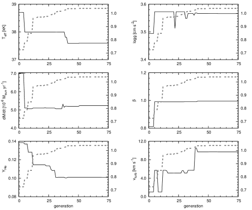
Figure 1: Evolution of the best fitting model parameters for formal test B. From the 200 generation run only the first 75 generations are shown. For this specific data set the location of the global optimum is found within 50 generations. This is indicated by the highest fitness found during the run, which is shown as a grey dashed line and is scaled to the right vertical axis. The fitness is normalized with respect to the fitness of the model used to create the synthetic data (the data being this model plus noise).

2.6 Formal tests of convergence

Before we apply our automated fitting method to real spectra, we first test whether the method is capable of global optimization. For this we perform convergence tests using synthetic data. The main goal of these tests is to determine how well and how fast the input parameters, used to create the synthetic data, can be recovered with the method. The speed with which the input parameters are recovered, i.e. the number of generations needed to find the global optimum, can then be used to determine how many generations are needed to obtain the best fit for a real spectrum. In other words, when the fit has converged to the global optimum.

Three synthetic datasets, denoted by A, B and C, were created with the following procedure. First, line profiles of Balmer hydrogen lines and helium lines in the optical blue and H$\alpha$ in the red calculated by fastwind were convolved with a rotational broadening profile. Table 1 lists the parameters of the three sets of models as well as the projected rotational velocity used. A second convolution with a Gaussian instrumental profile was applied to obtain a spectral resolution of 0.8 Å and 1.3 Å for, respectively, the H$\alpha$ line and all other lines. These values correspond to the minimum resolution of the spectra fitted in Sect. 3. Finally, Gaussian distributed noise, corresponding to a signal to noise value of 100, was added to the profiles. Dataset A represents an O3 I star with a very dense stellar wind ($\mbox{$\dot{M}$}=10^{-5}\,\mbox{$M_{\sun}{\rm yr}^{-1}$}$), while set B is that of an O5.5 I with a more typical O-star mass loss. The last set C is characteristic for a B0 V star with a very tenuous wind of only $10^{-8}\,\mbox{$M_{\sun}{\rm yr}^{-1}$}$.

From the synthetic datasets we fitted nine lines, three hydrogen, three neutral helium and three singly ionized helium lines, corresponding to the minimum set of lines fitted for a single object in Sect. 3. The fits were obtained by evolving a population of 72 fastwind models over a course of 200 generations. In this test and throughout the remainder of the paper we use pikaia with a dynamically adjustable mutation rate, with the minimum and maximum mutation rate set to the default values (see Charbonneau & Knapp 1995). Selection pressure, i.e. the weighting of the probability an individual will be selected for reproduction based on its fitness, was also set to the default value.

Table 1 lists the parameter ranges in which the method was allowed to search, i.e. the minimum and maximum values allowed for the parameters of the fastwind models. As $v_{\infty}$ and $v_{\rm r}\sin i$ are not free parameters these were set equal to the input values.

In all the three test cases the automated method was able to recover the global optimum. Table 1 lists the parameters of the best fit models obtained by the method in the “Out” columns. Compared to the parameters used to create the synthetic data, there is very good agreement. Moderate differences (of a 15-20% level) are found for $v_{\rm turb}$ recovered from dataset A and for the wind parameters $\beta$ and $\dot{M}$ recovered from dataset C. This was to be expected. In the case of the wind parameters the precision with which information about these parameters can be recovered from the line profiles decreases with decreasing wind density (e.g. Puls et al. 1996). Still, the precision with which the wind parameters are recovered for the weak wind data set C, is remarkable.

A similar reasoning applies for the microturbulent velocity recovered from data set A. For low values of the microturbulence, i.e. $\mbox{$v_{\rm turb}$}<v_{\rm th}$, thermal broadening will dominate over broadening due to microturbulence. This decreases the precision with which this parameter can be recovered from the line profiles. Realizing that in case of this dataset for helium $v_{\rm th}\leavevmode\nobreak\ \approx\leavevmode\nobreak\ 14\leavevmode\nobreak\ \mbox{km\,s${}^{-1}$}$, again, the precision with which $v_{\rm turb}$ is recovered, is impressive.

To illustrate how quickly and how well the input parameters are recovered Fig. 1 shows the evolution of the fit parameters during the fit of synthetic dataset B. Also shown, as a grey dashed line, is the fitness of the best fitting model found, during the run. This fitness is normalized with respect to the fitness of the model used to create the synthetic data (the data being the combination of this model and noise). Note that the final maximum normalized fitness found by the method exceeds 1.0, which is due to the added noise allowing a further fine tuning of the parameters by the GA based optimization. As can be seen in this figure the method modifies multiple parameters simultaneously to produce a better fit. This allows for an efficient exploration of parameter space and, more importantly, it allows for the method to actually find the global optimum.

In the case of dataset B finding the global optimum required only a few tens of generations ($\sim$30). For the other two datasets all save one parameter were well established within this number of generations. To establish the very low value of $v_{\rm turb}$ in dataset A and the very low $\dot{M}$ in dataset C required $\sim$100 generations. We will adopt 150 generations to fit the spectra in Sect. 3. One reason, obviously, is that to safeguard that the global optimum is found. A second reason, however, is that it assures that the errors on the model parameters that we determine are meaningful (i.e. it assures that the error on the error is modest).

We consider doing such a formal test as performed above as part of the analysis of a set of observed spectra, as the exact number of generations required is, in principle, a function of e.g. the signal-to-noise ratio and the spectral resolution. Also, special circumstances may play a role, such as potential nebular contamination (in which case the impact of removing the line cores from the fit procedure needs to be assessed).

Table 2: Basic parameters of the early type stars studied here. Spectral types are taken from Massey & Thompson (1991), Walborn (1972, 1973) and Conti & Alschuler (1971). Blue and red resolution, respectively, correspond to the region between $\sim$4000 and $\sim$5000 Å and the region around H$\alpha$.

Star	Spectral	$M_{V}$	Blue	Red	$v_{\rm r}\sin i$	$v_{\infty}$
	Type		resolution [Å]	resolution [Å]	[km s-1]	[km s-1]
Cyg OB2~#7	O3 If∗	$-5.91$	0.6	0.8	105	3080
Cyg OB2~#11	O5 If+	$-6.51$	1.3	0.8	120	2300
Cyg OB2~#8C	O5 If	$-5.61$	1.3	0.8	145	2650
Cyg OB2~#8A	O5.5 I(f)	$-6.91$	0.6	0.8	130	2650
Cyg OB2~#4	O7 III((f))	$-5.44$	1.3	0.8	125	2550
Cyg OB2~#10	O9.5 I	$-6.86$	0.6	0.8	95	1650
Cyg OB2~#2	B1 I	$-4.64$	0.6	0.8	50	1250
HD 15629	O5 V((f))	$-5.50$	0.6	0.8	90	3200
HD 217086	O7 Vn	$-4.50$	0.6	0.8	350	2550
10 Lac	O9 V	$-4.40$	0.6	0.6	35	1140
$ζ$ Oph	O9 V	$-4.35$	0.6	0.8	400	1550
$τ$ Sco	B0.2 V	$-3.10$	0.2	0.2	5	2000

3 Spectral analysis of early-type stars

In this section we apply our fitting method to seven stars in the open cluster Cyg OB2, previously analysed by Herrero et al. (2002) and five “standard” early-type stars, 10 Lac, $\tau$ Sco, $\zeta$ Oph, HD 15629 and HD 217086, previously analysed by various authors.

3.1 Description of the data

Table 2 lists the basic properties of the data used for the analysis. All spectra studied have a S/N of at least 100. The spectral resolution of the data in the blue (regions between $\sim$4000 and $\sim$5000 Å) and the red (region around H$\alpha$) is given in Tab. 2.

The optical spectra of the stars in Cyg OB2 were obtained by Herrero et al. (1999) and Herrero et al. (2000). Absolute visual magnitudes of the Cyg OB2 objects were adopted from Massey & Thompson (1991), and correspond to a distance modulus of 11.2^m. Note that for object #8A Tab. 7 in Massey & Thompson contains an incorrect $V_{0}$ value of 4.08^m. This should have been 4.26^m conform the absorption given in this table and the visual magnitude in their Tab. 2. For $v_{\rm r}\sin i$ values determined by Herrero et al. (2002) are used, with the exception of objects #8A and #10. For these we found that the He i and metal lines are somewhat better reproduced if we adopt $v_{\rm r}\sin i$ that are higher by $\sim$35% and $\sim$10%, respectively. Terminal flow velocities of the wind have been obtained from UV spectra obtained with Hubble Space Telescope (cf. Herrero et al. 2001). Data of HD 15629, HD 217086 and $\zeta$ Oph are from Herrero et al. (1992) and Herrero (1993). For $M_{V}$, $v_{\infty}$ and $v_{\rm r}\sin i$ values given by Repolust et al. (2004) are adopted. The distances to these objects are based on spectroscopic parallaxes, except for $\zeta$ Oph which has a reliable Hipparcos distance (Schröder et al. 2004).

The spectrum of 10 Lac was obtained by Herrero et al. (2002). The absolute visual magnitude of this star is from Herrero et al. (1992). For $v_{\infty}$ we adopted the minimum value which is approximately equal to the escape velocity at the stellar surface of this object. For the projected rotational velocity we adopt 35 km s^-1. The blue spectrum of $\tau$ Sco is from Kilian (1992). The red region around H$\alpha$ was observed by Zaal et al. (1999). For $\tau$ Sco we also adopt the Hipparcos distance. This distance results in an absolute visual magnitude which is rather large for the spectral type of this object, but is in between the $M_{V}$ adopted by Kilian (1992) and Humphreys (1978). For the projected rotational velocity a value of 5 km s^-1 was adopted.

3.2 Lines selected for fitting and weighting scheme

For the analysis fastwind will fit the hydrogen and helium spectrum of the investigated objects. Depending on the wavelength range of the available data, these lines comprise for hydrogen the Balmer lines H$\alpha$, H$\beta$, H$\gamma$ and H$\delta$; for He i the singlet lines at 4387 and 4922 Å, the He i triplet lines at 4026, which is blended with He ii, 4471 and 4713 Å; and finally for He ii the lines at 4200, 4541 and 4686 Å.

For an efficient and reliable use of the automated method we have to incorporate into it the expertise that we have developed in the analysis of OB stars. The method has to take into account that some lines may be blended or that they cannot be completely reproduced by the model atmosphere code for whatever reason For example, the so-called “generalized dilution effect” Voels et al. (1989), present in the He i $\lambda$4471 line in late type supergiants, that is still lacking an explanation.

Table 3: Line weighting scheme adopted for different spectral types and luminosity classes for the objects fitted in this paper. Late, mid and early spectral type correspond to, respectively, [O2-O5.5], [O6-O7.5] and [O8-B1]. The weights are implemented in the fitness definition according to Eq. (6) and have values of 1.0, 0.5 and 0.25 in case of h, m and l, respectively.

	Dwarfs				Super Giants
	Late	Mid	Early		Late	Mid	Early
H Balmer	h	h	h		h	h	h
He i  singlets	h	l	l		h	l	l
He i  4026	h	h	h		h	h	h
He i  4471	h	h	h		l	m	h
He i  4713	h	h	h		h	h	h
He ii 4686	h	m	m		m	m	m
He ii 4541	h	h	h		h	h	h
He ii 4200	m	m	m		m	m	m

To that end we have divided the stars in two classes (“dwarfs” and “supergiants”, following their luminosity class classification), and three groups in each class (following spectral types). We have then a total of six stellar groups, and have assigned the spectral lines different weights depending on their behaviour in each stellar group. This behaviour represents the expertise from years of “by eye” data analysis that is being translated to the method. Three different weights are assigned to each line: high, to lines very reliable for the analysis; medium, and low. The implementation of these weights into the fitness definition is given by

$$F\equiv\left(\sum_{i}^{N}w_{i}\chi_{{\rm red},i}^{2}\right)^{-1}\leavevmode\nobreak\ ,$$ (6)

where the parameter $w_{i}$ corresponds to the weight of a specific line.

Table 4: Results obtained for the investigated early type stars using GA optimized spectral fits. The spectra were fitted by evolving a population of 72 fastwind models over a course of 150 generations. Spectroscopic masses $M_{\rm s}$ are calculated with the gravities corrected for centrifugal acceleration $\log g_{\rm c}$. Evolutionary masses $M_{\rm ev}$ are from Schaller et al. (1992). The error bars on the derived parameters are given in Tab. 5 and are discussed in Sect. 4.

Star	$T_{\rm eff}$	$\log{{g}}$	$\log{{g}}_{\rm c}$	$R_{\star}$	$\log\mbox{$L_{\star}$}$	$Y_{\rm He}$	$v_{\rm turb}$	$\dot{M}$	$\beta$	$M_{\rm s}$	$M_{\rm ev}$
	[kK]	[cm s-2]	[cm s-2]	[$R_{\sun}$]	[$L_{\sun}$]		[km s-1]	[$M_{\sun}{\rm yr}^{-1}$]		[$M_{\sun}$]	[$M_{\sun}$]
Cyg OB2 #7	45.8	3.93	3.94	14.4	5.91	0.21	19.9	9.98$\cdot 10^{-6}$	0.77	65.1	67.8
Cyg OB2 #11	36.5	3.62	3.63	22.1	5.89	0.10	19.8	7.36$\cdot 10^{-6}$	1.03	75.9	55.6
Cyg OB2 #8C	41.8	3.73	3.74	13.3	5.69	0.13	0.5	3.37$\cdot 10^{-6}$	0.85	36.0	49.2
Cyg OB2 #8A	38.2	3.56	3.57	25.6	6.10	0.14	18.3	1.04$\cdot 10^{-5}$	0.74	89.0	74.4
Cyg OB2 #4	34.9	3.50	3.52	13.7	5.40	0.10	18.9	8.39$\cdot 10^{-7}$	1.16	22.4	32.5
Cyg OB2 #10	29.7	3.23	3.24	29.9	5.79	0.08	17.0	2.63$\cdot 10^{-6}$	1.05	56.0	45.9
Cyg OB2 #2	28.7	3.56	3.57	11.3	4.88	0.08	16.5	1.63$\cdot 10^{-7}$	0.801)	17.0	18.7
HD 15629	42.0	3.81	3.82	12.6	5.64	0.10	8.6	9.28$\cdot 10^{-7}$	1.18	37.8	47.4
HD 217086	38.1	3.91	4.01	8.30	5.11	0.09	17.1	2.09$\cdot 10^{-7}$	1.27	25.7	28.5
10 Lac	36.0	4.03	4.03	8.27	5.01	0.09	15.5	6.06$\cdot 10^{-8}$	0.801)	26.9	24.9
$\zeta$ Oph	32.1	3.62	3.83	8.9	4.88	0.11	19.7	1.43$\cdot 10^{-7}$	0.801)	19.5	20.3
$\tau$ Sco	31.9	4.15	4.15	5.2	4.39	0.12	10.8	6.14$\cdot 10^{-8}$	0.801)	13.7	16.0

¹⁾ assumed fixed value

Table 2 gives the weights assigned to each line in each stellar group. We will only briefly comment on the low or medium weights. He i singlets are assigned a low weight for mid-type stars because of the singlet differential behaviour found between fastwind and cmfgen (Puls et al. 2005), while they are very weak for early-type stars. In these two cases therefore we prefer to rely on the triplet He i $\lambda$4471 line. To this line, however, a low weight is assigned at late-type Supergiants because of the above mentioned dilution effect.

He ii $\lambda$4686 is only assigned a medium weight (except for late type dwarfs), as this line is not always completely consistent with the mass-loss rates derived from Halpha. He ii $\lambda$4200 is sometimes blended with N iii $\lambda$4200, and sometimes it is not completely consistent with the rest of the He ii lines. He i and He ii lines at 4026 Å do overlap, but for both lines we find a consistent behaviour.

The highest weight is therefore given to the Balmer lines plus the He ii $\lambda$4541 and the He i/He ii 4026 lines, which define the He ionization balance with He i $\lambda$4471 or the singlet He i lines. Note however that, as discussed above, all lines fit simultaneously in a satisfactory way for our best fitting models.

3.3 Fits and comments on the individual analysis

In the following we will present the fits that were obtained by the automated method for our sample of 12 early type stars, and comment on the individual analysis of the objects. Listed in Tab. 4 are the values determined for the six free parameters investigated and quantities derived from these.

3.3.1 Analysis of the Cyg OB2 stars

The Cyg OB2 objects studied here were previously analysed by Herrero et al. (2002, hereafter HPN). We opted to reanalyse these stars (to test our method) as these stars have equal distances and have been analysed in a homogeneous way using (an earlier version of) the same model atmosphere code. In Sect. 5 we will systematically compare our results with those obtained by HPN. Here, we will incidentally discuss the agreement if this turns out to be relatively poor or if the absolute value of a parameter seems unexpected, and we wanted to test possible causes for the discrepancy.

Cyg OB2 #7

The best fit obtained with our automated fitting method for Cyg OB2 #7 is shown in Fig. 2. For all hydrogen lines fitted, including H$\delta$ not shown here, and all He ii lines the fits are of very good quality. Note that given the noise level the fits of the He i lines are also acceptable.

Interesting to mention is the manner in which the He i and He ii blend at 4026 Å is fitted. At first sight, i.e. “by eye”, it seems that the fit is of poor quality, as the line wings of the synthetic profile runs through “features” which might be attributed to blends of weak photospheric metal lines. However, the broadest of these features have a half maximum width of $\sim$70 km s^-1, which is much smaller than the projected rotational velocity of 105 km s^-1. Consequently, these features are dominated by pure noise.

Compared to the investigation of HPN we have partial agreement between the derived parameters. The mass loss rate, $T_{\rm eff}$ and to a lesser degree $\beta$ agree very well. For $\log{{g}}$ and the helium abundance we find, however, large differences. The $\log{{g}}$ value obtained here is $\sim$0.2 dex larger, which results in a spectroscopic mass of 65.1 $M_{\sun}$. A value which is in good agreement with the evolutionary mass of 67.8 $M_{\sun}$.

The helium abundance needed to fit this object is 0.21, which is considerably lower than the value obtained by HPN, who found an abundance ratio of 0.31. This large value still corresponds to a strong helium surface enrichment. An interesting question we need to address, is whether this is a real enrichment and not an artifact that is attributable to a degeneracy effect of $T_{\rm eff}$ and $Y_{\rm He}$. The latter can be the case, as no He i lines are present in the optical spectrum of Cyg OB2 #7. This issue can be resolved with our fitting method by refitting the spectrum with a helium abundance fixed at a lower value than previously obtained. If $T_{\rm eff}$ and $Y_{\rm He}$ are truly degenerate this would again yield a good fit, however for a different $T_{\rm eff}$.

Shown as dotted lines in Fig. 2 are the results of refitting Cyg OB2 #7 with a helium abundance fixed at the solar value. For this lower $Y_{\rm He}$ a $T_{\rm eff}$ that is lower by $\sim$2.1 kK was obtained. This was to be expected as for this temperature regime He iii is the dominant ionization stage. When consequently $Y_{\rm He}$ is reduced a reduction of the temperature is required to fit the He ii lines. The reduction of $T_{\rm eff}$ obtained is the maximum for which still a good fit of the hydrogen lines is possible and the He i lines do not become too strong. More importantly, in Fig. 2 it is shown that even with this large reduction of $T_{\rm eff}$ the He ii lines cannot be fitted. This implies that $T_{\rm eff}$ and $Y_{\rm He}$ are not degenerate and the obtained helium enrichment is real.

Figure 2: Comparison of the observed line profiles of Cyg OB2 #7 with the best fit obtained by the automated fitting method (dashed lines). Note that the He ii line at 6527.1 Å is not included in the fit and, therefore, disregarded by the automated method. Horizontal axis gives the wavelength in Å. Vertical axises give the continuum normalized flux and are scaled differently for each line. In this figure the dotted lines correspond to a fit obtained for a helium abundance fixed at 0.1. See text for further comments.

Figure 3: Same as Fig. 2, however for Cyg OB2 #11

Figure 4: Same as Fig. 2, however for Cyg OB2 #8C. Shown with a dotted line for H$\alpha$ and He ii $\lambda$4686 are the line profiles of a model with a 0.05 dex lower $\dot{M}$, which “by eye” fits the core of H$\alpha$. See text for further comments.

Figure 5: Same as Fig. 2, however for Cyg OB2 #8A. The dotted lines correspond to a model with a $\dot{M}$ higher by 0.04 dex. This mass loss rate was obtained by fitting the best fit model, found by the automated method, “by eye” to the H$\alpha$ core. Even though the fit obtained with the higher $\dot{M}$ results in a fit of H$\alpha$ which is more pleasing to the eye in the line core, this higher mass loss rate does not describe this object the best. This can be seen best from the reduced fit quality of the other hydrogen Balmer lines and the severe mismatch of He i $\lambda$4471. See text for further comments.

Cyg OB2 #11

Figure 3 shows the fit to Cyg OB2 #11. In general all lines are reproduced correctly. There is a slight under prediction of the cores of H$\gamma$ and He ii $\lambda$4541, a problem that was also pointed out by Herrero et al. (1992) and HPN. Possibly this is due to too much filling in of the predicted profiles by wind emission. Part of the He ii $\lambda$4541 discrepancy might be related to problems in the theoretical broadening functions (see Repolust et al. 2005).

The parameters obtained for this object, with exception of $\dot{M}$, are in agreement with the parameters derived by HPN. With our automated method a mass loss rate lower by $\sim$0.1 dex was obtained. Note that due to this lower value the behaviour of this object in terms of its modified wind momentum (cf. Sect. 5.4) is in better accord with that of the bulk of the stars investigated in this paper.

Figure 6: Same as Fig. 2, however for Cyg OB2 #4.

Figure 7: Same as Fig. 2, however for Cyg OB2 #10. The emission feature in the core of H$\alpha$ was not included in the fit. A subsequent test which did include this feature in the fit yielded the same parameters except for a small increase of $\dot{M}$ with 0.04 dex.

Cyg OB2 #8C

The best fit for Cyg OB2 #8C is shown in Fig. 4. Again, with exception of the mass loss rate, the parameters we obtain for this object are in good agreement with the findings of HPN. We do find a small helium abundance enhancement, whereas HPN found a solar value.

To fit the P Cygni type profile of He ii at 4686 Å, the automated method used a $\dot{M}$ which, compared to these authors, was higher by approximately 0.15 dex. This higher value for the mass loss rate results in a H$\alpha$ profile which, at first sight, looks to be filled in too much by wind emission. To assess whether this could correspond to a significant overestimation of the mass loss rate, we lowered $\dot{M}$ in the best fit model by hand until the core of H$\alpha$ was fitted. In Fig. 4 the resulting line profiles are shown as a dotted line for H$\alpha$ and He ii $\lambda$4686, which for this fit are the lines which visibly reacted to the change in mass loss rate. To obtain this fit “by eye” of the H$\alpha$ core, a reduction of $\dot{M}$ with merely 0.05 dex was required, showing that the mass loss rate was not overestimated by the automated method. Note that for this lower mass loss rate the fit of the He ii $\lambda$4686 becomes significantly poorer.

Cyg OB2 #8A

De Becker et al. (2004) report this to be a O6 I and O5.5 III binary system, therefore the derived parameters, in particular the spectroscopically determined mass, should be taken with care. However, as this paper also aims to test automated fitting we did pursue the comparison of this object with HPN, who also treated the system assuming it to be a single star.

We obtained a good fit for all lines except for the problematic He ii $\lambda$4686 line. The best fit is shown in Fig. 5. Again the H$\alpha$ core is not fitted perfectly. To determine how significant this small discrepancy is, we fitted the H$\alpha$ core in a similar manner as for Cyg OB2 #8C. To obtain a good fit “by eye” we find that $\dot{M}$ has to be increased by 0.04 dex, indicating the extreme sensitivity of H$\alpha$ to $\dot{M}$ in this regime. The profiles corresponding to the increased mass loss rate model are shown in Fig. 5 as dotted lines. It is clear that not only the “classical” wind lines react strongly to $\dot{M}$. All synthetic hydrogen Balmer line profiles show significant filling in due to wind emission for an increased mass loss, deteriorating the fit quality. Also the He i $\lambda$4471 line shows a decrease in core strength which is comparable to the decrease in the H$\alpha$ core. This reconfirms that in order to self-consistently determine the mass loss rate all lines need to be fitted simultaneously. Therefore, a small discrepancy in the H$\alpha$ core between the observed and synthetic line profile should not be considered a decisive reason to reject a fit.

Except for $Y_{\rm He}$ the obtained parameters agree with the results of HPN within the errors given by these authors. Similar to Cyg OB2 #8C we find a small helium enhancement.

Cyg OB2 #4

The final fit to the spectrum of Cyg OB2 #4 is presented in Fig. 6. We obtained good fits for all lines, with exception of the helium singlet at 4922 Å, for which the core is predicted too strong. However, recall that for this spectral type we assigned a relatively low weight to this line, for reasons explained in Sect. 3.2.

The parameters obtained from the fit agree well with the values of HPN, with exception of $\beta$, for which we find a value higher by $\sim$0.2. Note that HPN used a fixed value for $\beta$ to obtain their fit, whereas in this case the automated method self-consistently derived this parameter.

The spectroscopic mass implied by the obtained $\log{{g}}$ value is significantly smaller than the evolutionary mass of Cyg OB2 #4. However, within the error bars (Sect. 4) the two masses agree with each other.

Figure 8: Same as Fig. 2, however for Cyg OB2 #2. Shown with dotted lines for H$\alpha$ is the line profile of the best fit model with a $\dot{M}$ lower by a factor of 3. See text for further comments.

Cyg OB2 #10

In the final fit for this object, shown in Fig. 7, there are two problematic lines. First, for the He ii $\lambda$4686 line the core is predicted too strong. Even though compared to HPN the situation has improved considerably, the current version of fastwind still has difficulties predicting this line. Second, the predicted He i $\lambda$4471 is too weak. Possibly this is connected to the generalized dilution effect, for which we refer to Repolust et al. (2004) for a recent discussion.

In Fig. 7 we also see that the H$\alpha$ core of Cyg OB2 #10 exhibits an emission feature. For this analysis we assumed that is was nebular and, consequently, excluded it from the fit. To test what the effect would be if this assumption was incorrect, a fit was made with this feature included in the profile. It turned out that the only parameter which was affected in this test was $\dot{M}$, which showed a small increase of 0.04 dex.

Cyg OB2 #2

For Cyg OB2 #2 the automated method could not self-consistently determine $\beta$. Therefore, we fixed its value at a theoretically predicted $\beta=0.8$ (cf. Pauldrach et al. 1986). In Fig. 8 the best fit is shown. We obtained good fits for all lines. However, in the case of He i $\lambda$4471 we do see a small under prediction of the forbidden component at 4469 Å, which is likely related to incorrect line-broadening functions.

For $\log{{g}}$ and $\dot{M}$ the obtained fit parameters differ considerably from the findings of HPN. We first focus on mass loss for which we obtain the relatively low rate of $1.63\times 10^{-7}$ $M_{\sun}{\rm yr}^{-1}$  with an error bar in the logarithm of this value of $-0.15$ and $+0.12$ dex (see Tab. 5), given the quoted value of $\beta$. Our $\dot{M}$ value is approximately a factor two higher than the mass loss rate obtained by HPN. These authors noted that it was not possible to well constrain the mass loss rate of such a weak wind. Given the relatively modest errors indicated by our automated fitting method, we conclude that at least in principle our technique allows to determine mass loss rates of winds as weak as that of Cyg OB2 #2. We have added the phrase “in principle” as it assumes the notion of beta and a very reliable continuum normalization, which is in this is case different from the one used by HPN for the He ii 4541, He ii 4686 and H$\alpha$ lines. If this can not be assured, then systematic errors may dominate over the characteristic fitting error and the mass loss may be much less well constrained. Assuming the continuum location to be reliable, we illustrate the sensitivity of the spectrum to mass loss rates of $\sim$$10^{-7}$ $M_{\sun}{\rm yr}^{-1}$ by reducing the mass loss by a factor of three. The H$\alpha$ profile of this reduced mass loss model is shown in Fig. 8 as a dotted line. Comparison of these two cases shows that for winds of order $10^{-7}$ $M_{\sun}{\rm yr}^{-1}$ the line still contain considerable $\dot{M}$ information. Interestingly, if we would not take into consideration the line core of H$\alpha$ in our fitting method, we still recover the quoted mass loss to within three percent. We note that for our higher mass loss this object appears to behave well in the wind momentum luminosity relation (see Sect. 5.4), whereas HPN signal a discrepancy when using their estimated $\dot{M}$ value.

The $\log{{g}}$ value obtained in this study is 0.36 dex larger than the value obtained “by eye” by HPN. Judging from the very good fits obtained, there is no indication that the automated fit overestimated the gravity. The spectroscopic mass of 17.0 $M_{\sun}$ implied by the larger $\log{{g}}$ value, is also in good agreement with the evolutionary mass of Cyg OB2 #2, which is 18.7 $M_{\sun}$.

3.3.2 Analysis of well studied dwarf OB-stars

We have also reanalysed five well known and well studied dwarf OB-stars, sampling the range of O spectral sub-types, in order to probe a part of parameter space that is not well covered by the Cyg OB2 stars. HD 217086 and $\zeta$ Oph, for instance, are fast rotators with $v_{\rm r}\sin i$ = 350 and 400 km s^-1 respectively (see also Tab. 2). 10 Lac is a slow rotator, and $\tau$ Sco is a very slow rotator. The latter two stars also feature very low mass loss rates, moreover, the actual $\dot{M}$ values of these stars are much debated (see Martins et al. 2004). HD 15629 is selected because it appears relatively normal.

Figure 9: Same as Fig. 2, however for HD 15629.

Figure 10: Same as Fig. 2, however for HD 217086.

HD 15629

Apart from a slight over-prediction of the core strength in He ii $\lambda$4200, a very good fit was obtained for this object. The final fit is presented in Fig. 9. This object has recently been studied by Repolust et al. (2004, hereafter RPH). Compared to the parameters obtained by these authors, we find good agreement except for $T_{\rm eff}$, $\dot{M}$ and $\beta$. Note that in contrast to this study we do not find a helium deficiency. However, the difference of 0.02 with respect to the solar value obtained here is within the error quoted by RPH.

The difference in wind parameters can be explained by the value of $\beta=0.8$ assumed by RPH. Our self-consistently derived value for $\beta=1.18$. As the effect of $\beta$ on the spectrum is connected to the mass loss rate through the velocity law and the continuity equation, the lower $\dot{M}$ obtained with the automated method is explained.

The 1.5 kK increase of $T_{\rm eff}$ compared to RPH can be attributed to the improved fit quality and the increase in $\log{{g}}$ of 0.1 dex. An increase in $\log{{g}}$ implies an increase in electron density, resulting in an increase in the recombination rate. The strength of both the He i and He ii lines depend on this rate, as the involved levels are mainly populated through recombination. Consequently, as He iii is the dominant ionization stage in the atmosphere of HD 15629 the strength of the He i and He ii lines will increase when the recombination rate increases. To compensate for this increase in line strength an increase in $T_{\rm eff}$, decreasing the ionization fractions of He i and He ii, is necessary.

HD 217086

With a projected rotational velocity of 350 km s^-1 this object can be considered to be a fast rotator, and our analysis of this object will show how well the automated method can handle large $v_{\rm r}\sin i$. In Fig. 10 the best fit obtained with our method is presented. We find that the large projected rotational velocity does not pose any problem for the method, i.e. the fit quality of all the lines fitted is very good.

With respect to the obtained parameters, again, these can be compared to the work of RPH. In this comparison we find considerable differences for $T_{\rm eff}$ and $\log{{g}}$ and a small difference for $Y_{\rm He}$. The effective temperature found by the automated method is 2.1 kK higher. This is a significant increase, but when the $\log{{g}}$ value obtained here is considered, this can be explained in a similar manner as the $T_{\rm eff}$ increase of HD 15629.

Figure 11: Same as Fig. 2, however for 10 Lac.

Figure 12: Same as Fig. 2, however for $\zeta$ Oph.

The best fit is obtained with a $\log{{g}}$ value that is 0.29 dex higher than the value from RPH. Judging from the line profiles in Fig. 10 there is no evidence for an overestimation of $\log{{g}}$. This higher $\log{{g}}$ removes the discrepancy with the calibration of Markova et al. (2004) found by RPH (see Fig. 17 in RPH). We also note that, similar to Cyg OB2 #2, the increased $\log{{g}}$ implies a spectroscopic mass which agrees well with the evolutionary mass of HD 217086 (cf. Tab. 4). This is not the case for the value determined by RPH, which points to a clear discrepancy.

The considerable helium abundance enhancement found by RPH is not reproduced by the automated method. Even though this object is a rapid rotator, our fit indicates a normal, i.e. solar, helium abundance.

10 Lac

Like in the case of Cyg OB2 #2, and for the remaining objects, the wind is too weak to self-consistently determine $\beta$. Therefore, again a value of $\beta=0.8$ was assumed.

The photospheric parameters obtained for 10 Lac agree very well with the results of HPN. The best fit to the observed spectrum is shown in Fig. 11. Whereas HPN find that the mass loss rate cannot be constrained and only an upper limit of $10^{-8}$ $M_{\sun}{\rm yr}^{-1}$ is found, the automated method was able to self-consistently determine $\dot{M}$ at $6\times 10^{-8}$ $M_{\sun}{\rm yr}^{-1}$, though with large error bars (see Tab. 5). Our error bar indicates that $\dot{M}$ may be an order of magnitude lower, i.e. it may still be consistent with the HPN result.

Figure 13: Same as Fig. 2, however for $\tau$ Sco.

Various other authors have determined the mass loss rate of 10 Lac using different methods. These determinations range from up to $2\times 10^{-7}$ (Howarth & Prinja 1989) down to $2\times 10^{-9}\leavevmode\nobreak\ \mbox{$M_{\sun}{\rm yr}^{-1}$}$ (Martins et al. 2004). Consequently, compared to these independent determinations no conclusive answer can be given to the question whether the $\dot{M}$ derived from the optical spectrum is correct. We conclude that the mass loss rate of 10 Lac is anomalously low when placed into context with the other dwarfs stars studied here. For instance, the dwarfs $\zeta$ Oph and HD 217086, which have luminosities that are, respectively, lower and higher by $\sim$0.1 dex, both exhibit a mass loss rate higher by several factors. In Sect. 5.4 we will discuss this further in terms of the wind-momentum luminosity relation.

$\zeta$ Oph

The large $v_{\rm r}\sin i$ of 400 km s^-1 was not a problem to obtain a good fit. In Fig. 12 the best fit for $\zeta$ Oph is presented. With the exception of the helium abundance, the comparison with the results of RPH yields very good agreement. Note that the mass loss rate obtained by these authors is an upper limit, whereas in this study $\dot{M}$ could be derived self-consistently. With respect to $Y_{\rm He}$ we do not find any evidence for a significant overabundance of helium, in agreement with Villamariz & Herrero (2005).

$\tau$ Sco

The best fit for $\tau$ Sco is presented in Fig. 13. All lines, including H$\delta$, which is not shown here, are reproduced accurately. The photospheric parameters we obtained can be compared to the work of Schönberner et al. (1988) and Kilian et al. (1991) who both studied $\tau$ Sco using plane parallel models. Kilian et al. found $T_{\rm eff}$=31.7 kK and $\log{{g}}$=4.25, whereas Schönberner et al. obtained $T_{\rm eff}$=33.0 kK and $\log{{g}}$=4.15. The difference in $T_{\rm eff}$ between the two studies is explained by the fact that in the latter analysis no line blanketing was included in the models. Therefore, we prefer to compare our $T_{\rm eff}$ to the former investigation, which agree very well. In terms of the gravity we find good agreement with the second study. The value obtained by Kilian et al. seems rather high. Given the almost perfect agreement between the synthetic line profiles and the observations in Fig. 13, the reason for this discrepancy is unclear. On a side note, more recently Repolust et al. (2005) analysed the infrared spectrum of this object. Their findings do confirm our lower value, but could not reproduce the enhanced helium abundance we find, due to a lack of observed infrared He ii lines.

In the recent literature the mass loss rate usually adopted for $\tau$ Sco is $9\times 10^{-9}$ $M_{\sun}{\rm yr}^{-1}$, which is considerably smaller than the $6.14\times 10^{-8}$ $M_{\sun}{\rm yr}^{-1}$ obtained in this study. However, the former mass loss rate is an average value determined by de Jager et al. (1988), based on the mass loss rates independently found by Gathier et al. (1981) and Hamann (1981). Based on the UV resonance lines, these two studies, respectively, determined $\dot{M}$ to be $7.4\times 10^{-8}$ and $1.3\times 10^{-9}$ $M_{\sun}{\rm yr}^{-1}$. So, they differ by more than a factor of 50. The mass loss rate obtained with the automated method is in reasonable agreement with that obtained by Gathier et al.. Our higher value is also supported by the study of the infrared spectrum of $\tau$ Sco by Repolust et al. (2005) who find $\mbox{$\dot{M}$}\simeq 2\times 10^{-8}\leavevmode\nobreak\ \mbox{$M_{\sun}{\rm yr}^{-1}$}$. Detailed fitting of Br$\alpha$ will likely clarify this issue.

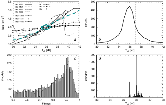
Figure 14: Panel a: fit diagram of $T_{\rm eff}$ and $\log{{g}}$ for 10 Lac. Panel b: Fitness as a function of $T_{\rm eff}$ for $\mbox{$\log{{g}}$}\ =4.0$. Panel c: Fitness distribution of the models calculated during the fitting run of the automated method. Panel d: Distribution of $T_{\rm eff}$ in the models located within the global optimum. The maximum variation of $T_{\rm eff}$ within the global optimum, which corresponds to the error estimate of this parameter, is $\sim$900 K.

4 Error analysis

Here we will introduce our method of estimating errors on the parameters derived with the automated method. This method is based on properties of the distribution of the fitnesses of the models in parameter space, which may seem conceptually different from classical approaches of defining error bars (and in a sense it is). However, we will demonstrate for the case of 10 Lac that our error definition is very comparable to what is routinely done in fit diagram approaches.

4.1 Fit diagrams

In a fit diagram method the error bar on $T_{\rm eff}$ and $\log{{g}}$ is derived by investigating the simultaneous behaviour of these two parameters. In panel a of Fig. 14 the fit diagram of 10 Lac is presented adopting for all other parameters (save $T_{\rm eff}$ and $\log{{g}}$) the best fit values obtained in our automated fitting. This diagram was constructed by calculating a grid of fastwind models in the $T_{\rm eff}$-$\log{{g}}$ plane, and evaluating for every line for every $T_{\rm eff}$ which model, i.e. $\log{{g}}$, fits this line the best. The location where the resulting fit curves intersect, corresponds to the best fit. This best fit yields $T_{\rm eff}$ = 36 000 K and $\log{{g}}$ = 4.0. Note that this result was obtained without the use of our automated method. The error can now be estimated by estimating the dispersion of the fit curves around this location. In panel a of Fig. 14 this is indicated by a box around the best fit location. The corresponding error estimates are 1000 K in $T_{\rm eff}$ and 0.1 dex in $\log{{g}}$.

The method described above cannot be applied to our automated fitting method due to two reasons. First, as we have defined the fit quality according to Eq. (1), this definition of fitness compresses the fit curves of all individual lines in the fit diagram to a single curve. In Fig. 14 this curve is shown as a thick dashed line. Although the curve runs through the best fit point, no information about the dispersion of the solutions around this point can be derived from it. The second reason lies in the multidimensional character of the problem of line fitting. If one would want to properly estimate the error taking this multidimensionality in to account, a fit diagram should be constructed with a dimension equal to the number of free parameters evaluated. In case of our fits this translates to the construction of a six dimensional fit diagram.

4.2 Optimum width based error estimates

Even though we have argued that fit diagrams cannot be used with our fitting method, it is possible to construct an error estimate which is analogous to the use of these diagrams and does take the multidimensionality of the problem into account. This can be done by first realizing that the error box shown in Fig. 14 essentially is a measure of the width of the optimum in parameter space, i.e. it defines the region in which models are located which approximately have the same fit quality. This is illustrated in panel b. There we show the one-dimensional fitness function in the $T_{\rm eff}$-$\log{{g}}$ plane for $\mbox{$\log{{g}}$}=4.0$. Indicated with dashed lines is the error in $T_{\rm eff}$ estimated using the fit diagram of 10 Lac. Confined between these lines is the region which corresponds to the optimum as defined by the error box in panel a. Consequently, the difference between maximum and minimum fitness in this region defines the width of the optimum. Returning to the general case, we can now invert the reasoning and state that the error estimate for a given parameter is equal to the maximum variation of this parameter in the group of best fitting models, i.e. the models located within the error box. Consequently, in the automated fitting method by defining a group of best fitting models, the error estimates for all free parameters can be determined.

Table 5: Error estimates for fit parameters obtained using the automated fitting method and parameters derived from these. Denoted by nd are errors in $v_{\rm turb}$ that reach up to the maximum allowed value of $v_{\rm turb}$ and, therefore, are formally not defined. Uncertainties in the fit parameters result from the optimum width based error estimates method. See text for details and discussion.

Star	$\Delta$$T_{\rm eff}$	$\Delta$$\log{{g}}_{\rm c}$	$\Delta$$R_{\star}$	$\Delta\log\mbox{$L_{\star}$}$	$\Delta$$Y_{\rm He}$	$\Delta$$v_{\rm turb}$	$\Delta\log$ $\dot{M}$	$\Delta$$\beta$	$\Delta$$M_{\rm s}$	$\Delta$$M_{\rm ev}$
	[kK]	[cm s-2]	[$R_{\sun}$]	[$L_{\sun}$]		[km s-1]	[$M_{\sun}{\rm yr}^{-1}$]		[$M_{\sun}$]	[$M_{\sun}$]
Cyg OB2 #7	${}^{-1.0}_{+1.5}$	${}^{-0.08}_{+0.06}$	$\pm$0.7	$\pm$0.07	${}^{-0.02}_{+0.03}$	${}^{-14.9}_{\rm+ND}$	${}^{-0.05}_{+0.03}$	${}^{-0.04}_{+0.09}$	${}^{-15}_{+12}$	${}^{-7}_{+7}$
Cyg OB2 #11	${}^{-0.6}_{+0.4}$	${}^{-0.07}_{+0.13}$	$\pm$1.1	$\pm$0.05	${}^{-0.01}_{+0.03}$	${}^{-4.0}_{\rm+ND}$	${}^{-0.03}_{+0.06}$	${}^{-0.05}_{+0.02}$	${}^{-15}_{+27}$	${}^{-3}_{+4}$
Cyg OB2 #8C	${}^{-1.3}_{+1.1}$	${}^{-0.10}_{+0.14}$	$\pm$0.7	$\pm$0.07	${}^{-0.02}_{+0.04}$	${}^{-0.2}_{+10.9}$	${}^{-0.07}_{+0.04}$	${}^{-0.05}_{+0.10}$	${}^{-10}_{+14}$	${}^{-4}_{+4}$
Cyg OB2 #8A	${}^{-0.4}_{+1.7}$	${}^{-0.05}_{+0.13}$	$\pm$1.3	$\pm$0.09	${}^{-0.04}_{+0.04}$	${}^{-17.7}_{\rm+ND}$	${}^{-0.07}_{+0.03}$	${}^{-0.04}_{+0.11}$	${}^{-15}_{+32}$	${}^{-10}_{+8}$
Cyg OB2 #4	${}^{-0.3}_{+1.5}$	${}^{-0.04}_{+0.21}$	$\pm$0.7	$\pm$0.09	${}^{-0.02}_{+0.03}$	${}^{-3.0}_{\rm+ND}$	${}^{-0.10}_{+0.05}$	${}^{-0.05}_{+0.21}$	${}^{-3}_{+15}$	${}^{-3}_{+3}$
Cyg OB2 #10	${}^{-0.8}_{+1.0}$	${}^{-0.12}_{+0.16}$	$\pm$1.5	$\pm$0.07	${}^{-0.02}_{+0.03}$	${}^{-7.0}_{\rm+ND}$	${}^{-0.13}_{+0.08}$	${}^{-0.15}_{+0.19}$	${}^{-19}_{+26}$	${}^{-4}_{+4}$
Cyg OB2 #2	${}^{-0.8}_{+1.2}$	${}^{-0.14}_{+0.13}$	$\pm$0.6	$\pm$0.08	${}^{-0.01}_{+0.03}$	${}^{-2.3}_{+2.4}$	${}^{-0.15}_{+0.12}$	-	${}^{-7}_{+6}$	${}^{-1}_{+2}$
HD 15629	${}^{-0.3}_{+0.7}$	${}^{-0.05}_{+0.07}$	$\pm$1.9	$\pm$0.12	${}^{-0.01}_{+0.03}$	${}^{-8.4}_{+7.6}$	${}^{-0.13}_{+0.10}$	${}^{-0.10}_{+0.27}$	${}^{-13}_{+14}$	${}^{-5}_{+7}$
HD 217086	${}^{-0.5}_{+0.9}$	${}^{-0.08}_{+0.07}$	$\pm$1.2	$\pm$0.13	${}^{-0.02}_{+0.02}$	${}^{-4.9}_{+2.9}$	${}^{-0.12}_{+0.18}$	${}^{-0.25}_{+0.16}$	${}^{-10}_{+10}$	${}^{-3}_{+3}$
10 Lac	${}^{-0.9}_{+0.8}$	${}^{-0.12}_{+0.13}$	$\pm$1.7	$\pm$0.17	${}^{-0.02}_{+0.02}$	${}^{-3.8}_{+4.1}$	${}^{-0.98}_{+0.39}$	-	${}^{-16}_{+16}$	${}^{-2}_{+4}$
$\zeta$ Oph	${}^{-0.7}_{+0.7}$	${}^{-0.05}_{+0.16}$	$\pm$1.3	$\pm$0.13	${}^{-0.02}_{+0.04}$	${}^{-6.2}_{\rm+ND}$	${}^{-0.28}_{+0.15}$	-	${}^{-7}_{+11}$	${}^{-2}_{+2}$
$\tau$ Sco	${}^{-0.8}_{+0.5}$	${}^{-0.14}_{+0.09}$	$\pm$0.5	$\pm$0.09	${}^{-0.02}_{+0.04}$	${}^{-2.2}_{+2.4}$	${}^{-0.99}_{+0.22}$	-	${}^{-6}_{+4}$	${}^{-1}_{+1}$

We define the group of best fitting models as the group of models that lie within the global optimum. Put differently, the width of the global optimum in terms of fitness, defines the group of best fitting models. Identifying and, consequently, measuring this width is facilitated by the nature of the GA, i.e. selected reproduction, incorporated in our fitting method. Due to this selected reproduction the exploration through parameter space results in a mapping of this space in which regions of high fit quality, i.e. the regions around local optima and the global optimum, are sampled more intensively. Consequently, if we would rank all models of all generations calculated during a fitting run according to their fitness, the resulting distribution will peak around the locations of the optima. In case of the global optimum the width of this peak, starting from up to the maximum fitness found, is, analogous to the width of the error box used in a fit diagram, a direct measure of the width of the optimum. Consequently, this width depends on the quality of the data, i.e. it will be broader or narrower for, respectively, low and high signal to noise, and on the degeneracy between the fit parameters. Therefore, the error estimates of the individual parameters are equal to the maximum variations of these parameters for all models contained in the peak corresponding to the global optimum.

In panel c of Fig. 14 the distribution of the models according to their fitness calculated during the fitting run of 10 Lac using the automated method is shown. The fitnesses are normalized with respect to the highest fitness and only the top half of the distribution is shown. In this distribution two peaks are clearly distinguishable. The most pronounced peak is located at $F\approx 0.9$ and corresponds to the region around the global optimum. A second peak, corresponding to a region around a secondary optimum, is located at $F\approx 0.83$. To derive the error on the fit parameters we estimate the total width of the global optimum for 10 Lac to be $\sim$0.15, i.e. the range of $F=0.85...1.0$ corresponds to the width of the optimum. In panel d of Fig. 14 we show the resulting distribution of $T_{\rm eff}$ of the models within this global optimum. In this figure we see that the maximum variation, hence the error estimate, is $\sim$900 K, which is in good agreement with the value derived using the fit diagram of 10 Lac. For $\log{{g}}$ we also find an error estimate of $\sim$0.1 dex, which is also very similar to the value obtained with this diagram. The exact values as well as error estimates for all fit parameters of all objects are given in Tab. 5. It is important to note that our error analysis method also allows for an error estimate of parameters to which the spectrum does not react strongly. For 10 Lac this is clearly the case for the mass loss rate, for which we find large error bars.

4.3 Derived parameters

In Tab. 5 the errors on the derived parameters were calculated based on the error estimates of the fit parameters. Here we will elaborate on their derivation.

The error in the stellar radii is dominated by the uncertainty in the absolute visual magnitude. In case of the Cyg OB2 objects we adopt these to be 0.1^m conform the work of Massey & Thompson (1991). For HD 15629, HD 217086 and $\zeta$ Oph we use the uncertainty as given by RPH of 0.3^m. The distance to 10 Lac and $\tau$ Sco was measured by Hipparcos. Therefore, for these two objects we adopt the error based on this measurement, which, respectively, is 0.4 and 0.2^m. Together with the uncertainty in $T_{\rm eff}$ the uncertainty in $R_{\star}$ is calculated according to Eq. (8) of RPH, where we used the largest absolute uncertainty in $T_{\rm eff}$ for a given object.

To correct the surface gravity for centrifugal forces, a correction conform Herrero et al. (1992) was applied to the gravity determined from the spectral fits. This corrected value is given in Tab. 4. As shown by RPH this correction has a non negligible effect on the error in the resulting $\log{{g}}_{\rm c}$. Consequently, we used their estimate to calculate the total error estimate of $\log{{g}}_{\rm c}$ as given in Tab. 5. Using this error together with the uncertainty in $R_{\star}$ the resulting uncertainty in the spectroscopic mass was calculated.

For the calculation of the uncertainty in the stellar luminosity, we consistently adopted the largest absolute error in $T_{\rm eff}$. The resulting $\Delta\log\mbox{$L_{\star}$}$ as well as the uncertainty in $T_{\rm eff}$ have an effect on the evolutionary mass. We have estimated errors for this quantity using the error box spanned by $\Delta\log\mbox{$L_{\star}$}$ and $\Delta\log\mbox{$T_{\rm eff}$}$.

5 Comparison with previous results

Figure 15: Comparison of the effective temperatures obtained using automated fits (horizontal axis) and “by eye” fits. On the vertical axis the ratio of automated relative to “by eye” temperature determination is given. The dashed lines correspond to a four percent error usually adopted for “by eye” determined values.

In this section we will compare the results obtained with our automated fitting method with those from “by eye” fits (relevant references to the comparison studies are given in the previous section). This does not constitute a one-to-one comparison of the automated and “by eye” approach as this would require the use of identical model atmosphere codes as well as the same set of spectra, moreover, with identical continuum normalization. Potential differences can therefore not exclusively be attributed to the less bias sensitive automated fitting method. However, as we have applied our method to a sizeable sample of early type stars, the automated nature of it does assure that it is the most homogeneous study to date, i.e. without at least some of the biases involved in conventional analyses.

5.1 Effective temperature

In Fig. 15 a comparison of the effective temperatures determined in this study with $T_{\rm eff}$ values obtained with “by eye” fits, is presented. Indicated with dashed lines are the four percent errors usually adopted for “by eye” fitted spectra. With the exception of the outlier HD 217086 at 38.1 kK, the agreement is very good and no systematic trend is visible. From this plot we can conclude that the $T_{\rm eff}$ obtained with the automated fit is at least as reliable as the temperatures determined in the conventional way.

5.2 Gravities

In many cases the gravity obtained with the automated procedure is significantly higher than the values obtained with the conventional “by eye” fitted spectra. This is shown in Fig. 16, where we show as a function of the gravities obtained in this study the differences with the “by eye” determined values. Indicated with dashed lines in this figure is the 0.1 dex error in $\log{{g}}$ that is often assigned to a “by eye” fitting of the hydrogen Balmer line wings. It is important to note that this plot shows that there is no obvious trend in the differences, i.e. there appears no systematic increase as a function of $\log{{g}}$ present.

Figure 16: Gravities obtained with automated fits (horizontal axis) are compared to gravities determined from “by eye” fits. The vertical axis gives the difference of the logarithm of the two gravity determinations. Indicated by dashed lines are the 0.1 dex errors usually adopted for gravities determined “by eye”.

It is clear, however, that there are three outliers for which previous gravity determinations yield values that are at least 0.2 dex lower. These are in order of increasing gravity (as determined in this study): Cyg OB2 #2, Cyg OB2 #7 and HD 217086. For all three cases, previous spectroscopic mass determinations result in values that are about a factor of two less than the corresponding evolutionary masses. One reason for these discrepant gravity values can be traced to a difference between automated and “by eye” fitting. In “by eye” fitting, it is custom to prohibit the theoretical line flux in the wings of Balmer lines – specifically that at the position in the observed line wing where the profile curvature is maximal – to be below that of the observed flux. This constraint has been used by HPN for the Cyg OB2 stars; for HD 217086, we could not verify whether this was the case. The automated method does not apply this constraint. Therefore, as it strives for a maximum fitness, it tends to fit the curve through the signal noise as much as possible. This yields a higher gravity.

A second reason is connected to the multidimensional nature of the optimization problem. “By eye” fitting may not find the optimum fit, as in general it can not simultaneously deal in a sufficiently adequate way with all the free parameters of the problem. Consequently, some of the “by eye” fitted spectra do not correspond to the best fit possible. A good example in which this appears to be the case is HD 217086. With the automated fit we not only obtained a gravity that is higher by $\sim$0.3 dex, but also an effective temperature higher by 2.1 kK compared to the results of RPH. Consequently, as the ionization structure of the atmosphere depends heavily on this temperature, so does the gravity one obtains from a spectral fit for this temperature. As RPH obtained a gravity for a significantly lower effective temperature, the gravity obtained from their spectral fit likely corresponds to the value from a local optimum in parameter space.

5.3 Helium abundance and microturbulence

This analysis is the first in which the helium abundance and the microturbulent velocity have been treated as continuous free parameters. In the studies of HPN and RPH only two possible values for the microturbulent velocity were adopted. For the helium abundance an initial solar abundance was adopted, which was modified when no satisfying fit could be obtained for this abundance. Consequently, a comparison with these studies as was done for e.g. the gravities, is not possible. Instead we will only discuss whether the obtained values of these parameters are reasonable and comment on possible correlations with other parameters.

The helium abundances given in Tab. 4 show that no extreme values were needed by the fitting method to obtain a good fit. An exception to this may be $Y_{\rm He}$=0.21 obtained for Cyg OB2 #7. However, as discussed earlier this value is still significantly smaller than the $Y_{\rm He}$=0.3 obtained by HPN. With respect to a possible relation between the helium abundance and other parameters, only a small correlation between $T_{\rm eff}$ and $Y_{\rm He}$ is found for the supergiants. For these objects it appears (cf. Tab. 4) that the helium abundance increases with increasing effective temperature. However, as we only analysed six supergiants further investigation using a larger sample needs to be undertaken.

Also for the microturbulent velocities no anomalous values were needed to fit the spectra. The large error bars in the turbulent velocity quoted in Tab. 5, especially for the supergiants, show that the profiles are not very sensitive to this parameter. This is consistent with the study of Villamariz & Herrero (2000) and RPH. The nd entries given on some of the positive errors in the table indicate that they reach up to the maximum allowed value of $v_{\rm turb}$, which is 20 km s^-1. Therefore, they are formally not defined. The fact that some of the small scale turbulent velocities are close to this maximum value may indicate that they represent lower limits, though, again, this likely reflects that they are poorly constraint.

No correlation of the microturbulence with any of the other parameters is found. In particular not between $v_{\rm turb}$ and $\log{{g}}$ and $v_{\rm turb}$ and $Y_{\rm He}$. Various authors have hinted at such a correlation (e.g. Kilian 1992).

5.4 Wind parameters

The straightforward comparison of the mass loss rates obtained with the automated method with values determined from spectral fits “by eye” is shown in Fig. 17. With exception of $\tau$ Sco at $\log\mbox{$\dot{M}$}=-7.2$, for which the mass loss rate determined by Gathier et al. (1981) from UV line fitting serves as a comparison, all mass loss rates are compared to values determined from H$\alpha$ fitting. For this comparison we assume an error of 0.15 dex in the “by eye” determined values. This uncertainty corresponds to a typical error obtained from H$\alpha$ fitting and is shown in Fig. 17 as a set of dashed lines. With exception of 10 Lac and $\tau$ Sco, for which the mass loss rate determination is uncertain, this error is also comparable to the errors obtained with the automated method.

Figure 17: Difference between mass loss rate obtained by the automated method (given by the horizontal) axis and values determined by eye. A typical 0.15 dex error is indicated by the dashed lines. The two outliers at $\log\mbox{$\dot{M}$}\simeq-7.2$ and and $\log\mbox{$\dot{M}$}\simeq-6.8$, respectively, correspond to 10 Lac and Cyg OB2 #2.

Two objects show a relative increase in $\dot{M}$ which is much larger than the typical error. These are 10 Lac at $\log\mbox{$\dot{M}$}\simeq-7.3$ and Cyg OB2 #2 at $\log\mbox{$\dot{M}$}\simeq-6.8$. In the case of the latter we showed that the increase is due to a more efficient use of wind information stored in the line profiles by the automated method, which improves the relation of Cyg OB2 #2 with respect to the wind-momentum relation (see Sect. 6.2).

With respect to 10 Lac we already mentioned that a range of more than two orders of magnitude in mass loss rate has been found in different studies. Here we have made the comparison with the upper limit found by HPN, which corresponds to one of the lowest $\dot{M}$ determined for this object. If we would have compared our findings to the higher value obtained by Howarth & Prinja (1989), 10 Lac would be at $\Delta\mbox{$\dot{M}$}=-0.5$, i.e. the situation in Fig. 17 would be reversed. Consequently, the large difference for 10 Lac shown in this figure can not be assigned to an error in the automated method, but rather reflects our limited understanding of this object.

All in all, we can conclude that the general agreement between mass loss rates obtained with the automated method and “by eye” determinations is very good.

6 Implications for the properties of massive stars

With our automated method we have analysed a sizeable sample of early type stars in a homogeneous way, which allows a first discussion of the implications the newly obtained parameters may have on the mass and modified wind-momentum luminosity relation (WLR) of massive stars. A thorough discussion however needs to be based on a much larger sample, therefore at this point we keep the discussion general and the conclusions tentative.

6.1 On the mass discrepancy

Figure 18: Spectroscopic masses derived in this study compared to evolutionary masses from Schaller et al. (1992). With the gravities obtained from the automated fits no mass discrepancy is found and no systematic deviation between the spectroscopically derived masses and the evolutionary predicted masses can be observed.

The so called mass discrepancy was first noticed by Herrero et al. (1992). These authors found that the spectroscopic masses, i.e. masses calculated from the spectroscopically determined gravity, were systematically smaller than the masses predicted by evolutionary calculations. The situation improved considerably with the use of unified stellar atmosphere models (e.g. Herrero et al. 2002). However, as pointed out by Repolust et al. (2004) for stars with masses lower than 50 $M_{\sun}$ still a milder form of a mass discrepancy appears to persist.

Does the automated fitting method, employing the latest version of fastwind, help in resolving the mass discrepancy? In Fig. 18 we present a comparison of the spectroscopic masses calculated with the gravities obtained in this study, with masses derived by interpolating evolutionary tracks of Schaller et al. (1992). It is clear that with the new gravities the situation is very satisfying. All objects have spectroscopic and evolutionary masses which agree within the error bars.

For stars with masses below 50 $M_{\sun}$ a milder form of the mass discrepancy (as found by RPH; see their Fig. 20) could still be present, but with the present data no systematic offset between the two mass scales can be appreciated. Though we feel it may be premature to conclude that the present analysis shows that the mass discrepancy has been resolved, our results point to a clear improvement.

6.2 Wind-momentum luminosity relation

The modified stellar wind momentum (MWM) versus luminosity relation offers a meaningful way to compare observed wind properties with aspects and predictions of the theory of line driven winds (see Kudritzki & Puls 2000 for a comprehensive discussion). Without going into any detail, the modified wind momentum $\mbox{$D_{\rm mom}$}=\mbox{$\dot{M}$}\mbox{$v_{\infty}$}R_{\star}^{1/2}$ is predicted to be a power law of stellar luminosity.

$$\log\mbox{$D_{\rm mom}$}=x\log(\mbox{$L_{\star}$}/\mbox{$L_{\sun}$})+\log D_{\circ}\leavevmode\nobreak\ ,$$ (7)

where $x$, the inverse of the slope of the line-strength distribution function corrected for ionization effects (Puls et al. 2000), is expected to be a function of spectral type and metal abundance, and $D_{\circ}$ is a function of metallicity and possibly luminosity class (Markova et al. 2004). The advantageous property of $D_{\rm mom}$ is that it is not very sensitive to the stellar mass.

The limited number of stars studied in this paper is clearly insufficient to disentangle subtleties in the $D_{\rm mom}$ vs. $L_{\star}$ relation. However, it is interesting to compare the observed and predicted modified wind momentum, as well as to discuss the location of 10 Lac – a notorious outlier.

Figure 19: Modified wind momentum (MWM) in units of [g cm s^-2$R_{\sun}$] of the objects fitted with the automated method (solid dots). The solid line, giving the wind-momentum luminosity relation (WLR), corresponds to the regression of the modified wind momenta. Given by the dashed line is the predicted WLR of Vink et al. (2000).

Figure 19 shows this comparison between derived and theoretical modified wind momentum. Using all programme stars to construct an empirical linear curve in the units of this diagram gives the following relation

$$\log\mbox{$D_{\rm mom}$}=(1.88\pm 0.09)\log(\mbox{$L_{\star}$}/\mbox{$L_{\sun}$})+(18.59\pm 0.52)\leavevmode\nobreak\ .$$ (8)

Within the given errors this relation is equal to the theoretical WLR predicted by Vink et al. (2000), who found $x=1.83$ and $\log\mbox{$D_{\rm mom}$}=18.68$. Note that the low luminosity objects ($\log\mbox{$L_{\star}$}/\mbox{$L_{\sun}$}\lesssim 5.5$) also follow the average relation. Therefore, the newly obtained mass loss rates do not show the discrepancy found by Puls et al. (1996) and Kudritzki & Puls (2000), but confirm the work of RPH. These authors found the low luminosity objects to follow the general trend, based on upper limits they obtained for the mass loss rates, whereas our new method is sensitive enough to determine these self-consistently.

In order to investigate the effect of the anomalously low $D_{\rm mom}$ obtained for 10 Lac, we also constructed a WLR excluding this object. We found that for this new relation the parameters $x$ and $\log D_{\circ}$ only changed with $\sim$0.02 and $\sim$0.01, respectively, reflecting the large error bars found for this object.

Previous investigations by Markova et al. (2004) and RPH have found the WLR to be as function of luminosity class. Whereas the former study finds a steeper WLR for the supergiants compared to the dwarfs, the latter finds the opposite (though RPH remark that the subset of Cyg OB2 stars seem to behave more in accordance with the theoretical result). In our sample no obvious separation is visible. In particular note the two objects overlapping at $\log\mbox{$L_{\star}$}/\mbox{$L_{\sun}$}=4.9$ in Fig. 19, which are the dwarf $\zeta$ Oph and the supergiant Cyg OB2 #2. To investigate a possible separation in more detail, a separate WLR was constructed for the Cyg OB2 supergiants. The resulting values of the parameters obtained are $x=1.79\pm 0.14$ and $\log D_{\circ}=19.12\pm 0.80$. The decrease in $x$ qualitatively confirms the work of Markova et al.. However, we have to realize that our sample might be too small from a statistical point of view to be able to firmly conclude whether a real separation exists. Therefore, this question has to be postponed until we have analysed a larger sample.

7 Summary, conclusions and future work

We have presented the first method for the automated fitting of spectra of massive stars with stellar winds. In this first implementation, a set of continuum normalized optical spectral lines is fitted to predictions made with the fast performance non-LTE model atmosphere code fastwind by Puls et al. (2005). The fitting method itself is based on the genetic algorithm pikaia by Charbonneau (1995), which was parallelized in order to handle the thousands of fastwind models which have to be calculated for an automated fit. Concerning the automated method we can draw the following conclusions:

1. The method is robust. In applying the method to a number of formal tests, to the study of seven O-type stars in Cyg OB2, and to five Galactic stars including extreme rotators and/or stars with weak winds (few times $10^{-8}$ $M_{\sun}{\rm yr}^{-1}$) the fitting procedure did not encounter convergence problems.

2. Using the width of the global optimum in terms of fitness, defining the group of best fitting models, we are able to define error estimates for all of the six free parameters of the model ($T_{\rm eff}$, $\log{{g}}$, helium over hydrogen abundance, $v_{\rm turb}$, $\dot{M}$ and $\beta$). These errors compare well with errors adopted in “by eye” fitting methods.

3. For the investigated dataset our automated fitting method recovers mass-loss rates down to $\sim$ $6\times 10^{-8}\mbox{$M_{\sun}{\rm yr}^{-1}$}$ to within an error of a factor of two. We point out that even for such low mass-loss rates it is not only the core of the hydrogen H$\alpha$ line that is a mass-loss diagnostics. When ignoring this core the GA still recovers $\dot{M}$, showing that the GA is also sensitive to indirect effects of a change in $\dot{M}$ on the atmospheric structure as a whole. However, for the method to fully take advantage of this information a very accurate continuum normalization is required.

4. Though we have so far tested our method for O-type stars and early B-type dwarf stars, the method can also be applied to B and A supergiants when atomic models of diagnostic lines (such as Si iii and Si iv) are implemented into the analysis.

We have re-investigated seven O-type stars in the young cluster Cyg OB2 and compared our results with the study by Herrero, Puls, & Najarro (2002). The HPN study uses an earlier version of fastwind and a “by eye” fitting procedure. The only difference between the two studies in terms of the treatment of the free parameters is that HPN did not treat the microturbulent velocity and the hydrogen over helium abundance ratio as continuous free parameters. Instead, they opted to adopt in case of the former two possible values only. In case of the latter an initial solar abundance was adopted which was modified in case no satisfying fit could be obtained with this solar abundance. We have also compared the results of an automated fitting to five early-type dwarf stars to further investigate the robustness of our method for stars with high rotational velocities and/or low mass loss rates. With respect to weak winds we refer to conclusion iii. Regarding large $v_{\rm r}\sin i$ values, we find that these do not pose problems for the automated method. This is reflected in conclusion i. Concerning the spectral analysis of the entire sample we can draw the following conclusions:

1. For almost all parameters we find excellent agreement with the results of HPN and RPH, which, we note, make use of a previous version of fastwind and an independent continuum normalization. The quality of our fits (in terms of fitness, which is a measure for the $\chi^{2}$ of the lines) is even better than obtained in these prior studies.

2. In three cases we find a significantly higher surface gravity (by up to 0.36 dex). We identify two possible causes for this difference that may be connected to the difference between automated and “by eye” fitting. First, comparison of the two methods indicates that in fitting the Balmer line wings the latter method places essentially infinite strength to the observed flux at the point of maximum curvature of the wing profile. The automated method does not do this. Second, as the automated method is a multidimensional optimization method it may simply find a better fit to the overall spectrum. In at least one case this implied a higher temperature and significantly higher gravity.

3. A comparison of our derived masses with those predicted by evolutionary calculations does not show any systematic discrepancy. Such a discrepancy was first noted by Herrero et al. (1992), though was partly resolved when model atmospheres improved (e.g. see HPN). Still, with state-of-the-art models a mild form of a mass discrepancy remained for stars with masses below 50 $M_{\sun}$ (e.g. see RPH, ). The automated fitting approach in combination with the improved version of fastwind does not find evidence for a mass discrepancy, although we remark that a truly robust conclusion, particularly for stars between 20 and 50 solar masses, may require the investigation of a larger sample.

4. The empirical modified wind momentum relation constructed on the basis of the twelve objects analysed in this study agree to within the error bars with the theoretical MWM relations based on the Vink et al. (2000) predictions of mass loss rates.

This first implementation of a genetic algorithm combined with the fast performance code fastwind already shows the high potential of automatic spectral analysis. With the current rapid increase in observations of early-type massive stars the need for an automated fitting method is evident. We will first use our method to analyse the $\sim$100 O-type and early B-type stars observed in the VLT large programme FLAMES Survey of Massive Stars (Evans et al. 2005) in the Galaxy and the Magellanic Clouds in a homogeneous way. Future development of the automated fitting method is likely to be in conjunction with the further development of fastwind. Improvements will include the modeling of: near-infrared lines (see e.g. Lenorzer et al. 2004 and Repolust et al. 2005), optical CNO lines (see e.g. Trundle et al. 2004), and possibly UV resonance lines. Additional model parameters that may be constrained within an automated approach include a depth dependent profile for the microturbulent velocity and small scale clumping. Within the current implementation, most likely the method will also be able to constrain the terminal flow velocity of A-type supergiants (McCarthy et al. 1997; Kudritzki et al. 1999).