Neutron Catalysis of Resonance Fusion in Stellar Matter

Abstract

Within the framework of resonance fusion study in stellar matter the features of $n,\alpha,\alpha$ - system have been investigated at astrophysical energies. Consideration of three body scattering has been carried out on base of well-known Faddeev’s equations.

It is found that under certain conditions the series of resonance states appear in $n,\alpha,\alpha$ system at very low energies ($\sim keV$ ). The lifetimes of these three body resonances are close to the lifetime of unstable nucleus ${}^{8}Be$.

The ground state of $\alpha,\alpha$ - system is regarded as very narrow resonance with the energy $\sim 92$ keV and the width $\sim 6.8$ eV. The simple forms of two body repulsive potentials are taken into account to describe the parameters of the $\alpha,\alpha$ - resonance and to satisfy $n,\alpha$ scattering data at very low energies.

The explanation of resonance phenomena in $n,\alpha,\alpha$ - system is offered on base of physical model. The effect results from resonance quantum phenomena in few body dynamics.

In turn, the resonance fusion can give influence on many astrophysical phenomena. The possibility of catalyzing this new mode of fusion by free neutrons in $\alpha$-particle matter is considered too in present exposal.

Introduction

It is the well-known fact that F. Hoyle predicted the existence of narrow low energy resonance in the system of three $\alpha$-particles [1]. Then his prediction was confirmed by experiments. It caused the essential progress of nucleogenesis understanding in stellar interior [2] - [4].

The present exposal contributes to development of low energy resonance astrophysics, in particular, resonance phenomena in system consisted of two $\alpha$ - particles and one neutron. Consideration has been given to the new type of fusion reactions, which can take place in stellar matter. These reactions are resulted from resonance quantum phenomena in few body systems [5] - [7].

Note that neutron and $\alpha$ - particle can not form a bound state. Neutron of very low energy can not be captured by $\alpha$ - particle. Its effective potential of interaction is characterized as a repulsing power in S-wave component. However, attraction in P-wave components is sufficiently strong to result in resonance behavior of corresponding amplitudes near the energy of $\sim 1\ MeV$ [8].

Two $\alpha$ - particles can not be bound in a stable state but in scattering they have the very narrow resonance at low energy region. The resonance energy $\simeq 92\ keV$ and the width $\simeq 6.8\ eV$ [8]. Moreover, the system of three $\alpha$-particles has the resonance state of long lifetime too. The resonance energy and width are $\simeq 0.38\ MeV$ and $\simeq 8.5\ eV$, respectively, in this case [9].

We have found that three body system consisting of two $\alpha$-particles and one neutron has a set of narrow resonances situated under the ground state energy of their subsystem - ${}^{8}Be$ [5]. The last one is considered as a sharp resonance.

In the system of three $\alpha$-particles and one neutron the number of similar resonances may be even more. So, it is proposed that a free neutron can gather few $\alpha$-particles to form quasi-molecular resonance states.

As for systems of few $\alpha$-particles the probability of resonance state formation at very low energies is small, and Coulomb barrier is also preventing it. Accompaniment of free neutron to the system of few $\alpha$ - particles mainly changes a situation. Amongst $\alpha$ - particles a neutron will play a role of interchanging particle, creating efficient additional attraction.

Therefore owing to free neutron the low energy fusions become possible with few $\alpha$-particles. They can product the different nuclei including nuclei with mass several times superior than $\alpha$ - particle’s mass.

The neutron can get free and then stimulate resonance reactions again. In the fusion reactions the neutron can be released taking a lot of the kinetic energy. The neutron is slowed down in an ambience of $\alpha$ - particles and then can form once again resonance quasi-molecular states.

Mechanism of neutron catalysis in resonance fusion reminds well known $\mu$ - catalysis in nuclear fusion of $\mu$, d, t - molecules [10].

It is assumed that inside stars there is presence of area with the high density of helium, where can occur described processes.

The resonance fusion can have influence on many astrophysical phenomena. Some of them are discussed below.

I General restrictions and Two body potentials

We consider a very low energy region - close to the temperature at the center of the Sun ($\ll 1MeV$). Relativistic effects, contributions of inelastic nuclear channels, quark structure of nucleons and nuclei etc are not taken into account. Nucleons and $\alpha$-particles are considered as nonstructural bodies. Effects of rearrangement between neutrons and nuclei are ignored. Thus, it is under consideration a very simple model to investigate the resonant phenomenon in three body dynamics.

In case of simple isolated resonance in two body system the amplitude of scattering has the distinctive form

$$f(E)\simeq\frac{-1}{\pi\rho(E)}\frac{\Gamma/2}{E-E_{R}+i\Gamma/2}.$$ (1)

It means that two-body amplitude has poles in $k$-complex plane in points of $k=k_{Res}=\pm k_{R}+ik_{I}$, where $E_{Res}=k_{Res}^{2}/2\mu$, $E_{R}=(k_{R}^{2}-k_{I}^{2})/2\mu$, $\Gamma=-4k_{R}k_{I}/2\mu$ and $k_{I}<0$, $\mu$ - reduced mass, $\rho(E)$ - the density of states in the continuum region.

Interactions between two particles are chosen in the simplest form - in form of separable potentials:

$$\{\lambda V\}_{L,S}^{J}=|\nu_{L,S}^{J}>\lambda_{L,S}^{J}<\nu_{L,S}^{J}|.$$ (2)

In this expression only a partial component of potential is written out. They satisfactory describe resonance behavior in pair subsystems [11]. Hereinafter the angular functions, recoupling coefficients, etc are omitted for the simplification. The quantum scattering theory of three-body system is given an account of [12]. Theory of quantum few-body systems with details can be found, for instance, in [13].

Using the separable potential gives an exact analytical solution of two-body problem. It is their obvious quality. The scattering amplitude can be written as:

$$f(k,k^{\prime};Z)=<k|\hat{f}|k^{\prime}>,\ \ \hat{f}=-|\nu>\eta(Z)<\nu|,\\$$ (3)

where

$$\eta^{-1}=\lambda^{-1}-A(Z),\ \ A=<\nu|G_{0}(Z)|\nu>,$$ (4)

and for simplicity indexes of states are omitted too. The amplitude $f(k,k^{\prime};Z)$ comes to the physical one $f(E)$ in limit $Z\rightarrow E=k_{0}^{2}/2\mu$, where $E$ - the real quantity and $|\vec{k}|=|\vec{k^{\prime}}|\rightarrow k_{0}$.

In case of potential (2) is represented as a sum of separable ones the expressions of (3) and (4) have to be understood as matrix values in relation to corresponding index.

The partial amplitude can get a pole in point of bound state $Z=E_{B}$, when $\lambda^{-1}=A(E_{B})$ and $E_{B}\leq 0$. But a pole may be in point of resonance state $Z=E_{Res}$, when $\lambda^{-1}=A(E_{Res})$ and $E_{Res}$ is a complex quantity [6].

It is convenient to normalize form-factors with condition $A(0)=-1$ appointing $\lambda$ as dimensionless constant.

A The separable $n,\alpha$-potentials

Effective potential of $n,\alpha$-interaction at low energy region has the following properties. Its S-wave component corresponds to repulsive force in accordance with Pauli principle. The S-wave potential represents the main factor in our case, i.e. at very low energies.

For S wave the form-factor of potential (2) can be chosen as:

$$<\nu_{n,\alpha}|k>=N^{S}_{n,\alpha}/(1+x^{2}),$$ (5)

where the constant $N^{S}_{n,\alpha}=\sqrt{8\pi/(2\mu\beta)}$, the variable $x=k/\beta$ and $\beta$ - the inverse radius of nuclear force.

It should be noted that in case of attractive force the equation $\lambda^{-1}=A(E_{B})$ gives a bound energy $E_{B}=-k_{I}^{2}/2\mu$, where $x_{I}=k_{I}/\beta=\kappa$, $\lambda=-(1+\kappa)^{2}$, $\kappa>0$ and $\lambda\leq-1$ .

In case of $-1<\lambda<0$ one can obtain a quantity for virtual state: $\kappa=-1+\sqrt{-\lambda}<0$.

In the contrary in case of the repulsive potential (2) with form-factor (5) the resonance state appears in the system. Potential parameters obey the following relationship: $x_{R}^{2}=k_{R}^{2}/\beta^{2}=\lambda>0$ and $k_{I}=-\beta<0$, which results from equation: $\lambda^{-1}=A(E_{Res})$.

So, the parameters fixed by $n,\alpha$ experimental scattering data are equal: $\beta=0.751fm^{-1}$ and $\lambda=14.94$. In turn they give the resonant energy and width such as: $E_{R}\sim\Gamma\sim 200\ MeV$ [6], [11].

Other components of effective $n,\alpha$-interaction correspond to the attraction forces, and the most important among them are P-wave interactions.

For P-waves ($P_{L,S}^{J}$, with $L=1$, $S=1/2$ and $J=3/2$ or $J=1/2$) the form-factor may be chosen, for example, in following forms:

$$<\nu^{P}_{n,\alpha}|k>=N^{P}_{n,\alpha}\frac{x}{1+x^{2}}\ ,\ \ \ or\ \ <\tilde{\nu}^{P}_{n,\alpha}|k>=\tilde{N}^{P}_{n,\alpha}\frac{x}{(1+x^{2})^{2}}\ .$$ (6)

Then, parameters of $n,\alpha$-system have to be in agreement with experimental data. For first of them ($J=3/2$) they are following: $x_{R}=k_{R}/\beta\simeq 0.158$, $x_{I}=k_{I}/\beta\simeq-0.0256$, $\beta=1.175fm^{-1}$ and $\lambda=-0.97$ that correspond to $E_{R}\simeq 0.9MeV$ and $\Gamma\simeq 0.6MeV$. It is easy to determine all parameters for whatever other case and another selection.

The description of low energy $n,\alpha$-scattering is sufficiently assigned by potentials of S- and P-waves up to energies $\simeq 10\ MeV$ [14], [15].

B The separable $\alpha,\alpha$-potentials

As it is known, no stable nuclei are consisted of 5 or 8 nucleons. For example, ${}^{8}Be$ has a lifetime $\sim 10^{-16}s$ [8]. Obviously, it is a huge time in relation to nuclear time scale.

Experimental data give parameters of this resonance: parity $0^{+}$, energy $92\ keV$ and width $6.8\ eV$ [8]. Note that the experimental data of $\alpha,\alpha$-resonance give the ratio

$$|k_{I}/k_{R}|\simeq 0.185\cdot 10^{-4}\ .$$ (7)

In general, effective potential of two $\alpha$-particles has to be a result of several complex interactions and involved forces. It is clear that a determination of exact potential is a very difficult problem of few-body physics to get solution even at low energies.

However, it is possible to describe this resonance within the framework of simple potential model like (2).

We consider this nucleus as a very narrow resonance in amplitude of two $\alpha$-particle $S$-wave scattering at low energies. That is why we will take into account only the corresponding part of total two body interaction and ignore other parts at very low energy region. These parts can become essential at higher energies. We’ll mark here the resonance state as $(\alpha,\alpha)^{*}$.

Below we can see that parameter of resonant quality (7) brings about suppression of such interactions.

Moreover, when viewed of interaction between a neutron and the $(\alpha,\alpha)^{*}$-system we ignore the Coulomb force too. We guess that resonant phenomena in $n,\alpha,\alpha$-system depend on features of neutron as neutral particle and $(\alpha,\alpha)^{*}$-subsystem as resonator.

Indeed, Coulomb repulsion is of particular importance for low-energy resonances, since it reduces the probability for charged particles to approach each other closely and, hence, the probability of their nuclear interactions. Moreover, Coulomb repulsion can deform a resonance substantially - for example, push it to the region of higher energies [16], [17].

Note, that problems of scattering governed by both Coulomb and nuclear forces have special features inherent in them that are due to the ”bad” behavior of Coulomb forces in the asymptotic region. This leads to the interplay of the nuclear and Coulomb transition operators, with the result that, even upon the separation of the purely Coulomb component from the total two-particle amplitude, the remainder involves irregular factors.

The situation becomes even more complicated in the problems where the scattering process involves three or more particles (see, for instance [18], [19]).

However, the problem of describing the properties of resonance scattering becomes more tractable in the energy region around a narrow resonance. First of all, this applies to a determination of the Coulomb shifts of resonance levels [6].

Our calculations carried out with Coulomb force between two $\alpha$-particles give a result of very small shift of resonance level in case of repulsive shot-range potentials [20].

Meanwhile in case of attractive shot-range potentials the Coulomb shifts of resonance levels can be very essensial [17].

In any case the resonant quality (7) can not be worse without Coulomb repulsive forces. It is a reason to consider a simple model of repulsive shot-range potentials ignoring Coulomb forces at first step of investigations.

Using S-wave potential form-factors for $(\alpha,\alpha)^{*}$-system in form:

$$<\nu^{(m)}_{\alpha,\alpha}|k>=N^{(m)}_{\alpha,\alpha}/(1+x^{2})^{m/2}\ ,$$ (8)

where $m=2,3,4,5$ and $6$, we can get exact solutions (3) and then determine corresponding potential parameters and quantities $x_{R}$, $x_{I}$ are being in accordance with experimental data.

As far as $m=2$ the form-factor (8) gives unreasonable values of $\beta$ and $\lambda$. In case of $m\geq 4$ parameters are more reasonable and within the sensible limits (see Table 1).

TABLE I.: Parameters of $(\alpha,\alpha)^{*}$ potentials with form-factors (8)

and corresponding resonance parameters.

m	2	3	4	5	6
$\lambda$	$2.9\cdot 10^{9}$	$1.08\cdot 10^{4}$	$9.06\cdot 10^{2}$	$3.13\cdot 10^{2}$	$1.75\cdot 10^{2}$
$\beta_{\alpha,\alpha}(fm^{-1})$	$1.75\cdot 10^{-6}$	$1.58\cdot 10^{-3}$	$0.7\cdot 10^{-2}$	$1.4\cdot 10^{-2}$	$2.12\cdot 10^{-2}$
$x_{R}$	$5.4\cdot 10^{4}$	60.0	13.5	6.73	4.46
$-x_{I}$	1	$1.11\cdot 10^{-3}$	$2.5\cdot 10^{-4}$	$1.25\cdot 10^{-4}$	$0.827\cdot 10^{-4}$

II Three interacting bodies

The quantum theory of three body scattering is excellently presented in classical monographs and reviews on few-bodies and related subjects (see, for instance [12], [13], [16], [18], [21] - [23]).

Here it’s enough to refer to needed formulas only for understanding and using in calculations.

So, the three-body system can be considered as the system of particles with simple pair interactions in form (2) with parameters specified in the preceding section. As usual, consideration has been carried out within the framework of Faddeev’s equations but using more convenient way - approach of effective potential [23], [24].

The amplitude of scattering of neutron on $\alpha,\alpha$-subsystem can be written as:

$$f_{i,j}=-<\varphi^{-}_{\alpha,\alpha^{\prime}}|(V_{n,\alpha}+V_{n,\alpha^{\prime}})|\Psi^{+}_{j}>\ ,$$ (9)

where $\varphi$ corresponds to the wave-function with one two-body interaction only, $\Psi^{\pm}_{j}$ - a total wave-function, where indexes $+(-)$ correspond to outcoming (incoming) waves. A total potential in our case is a sum of two-body potentials: $V=V_{\alpha,\alpha^{\prime}}+V_{n,\alpha}+V_{n,\alpha^{\prime}}=\sum V_{i}$, $i=1,2,3$. For example, index $j$ in (9) corresponds to final subsystem, i.e. marked a number of first particle left the interaction field in asimptotic.

Introducing $Q_{i,j}=V_{i}|\Psi_{j}>$ we get Faddeev’s equations in form:

$$Q_{i,j}=\tau_{i}\delta_{i,j}+\sum_{l=1}^{3}t_{i}G_{0}\overline{\delta}_{i,l}Q_{l,j}\ ,$$ (10)

where $\tau_{i}=V_{i}|\varphi_{i}>$, $t_{i}$ - the pair transition operator obeys $t_{i}=V_{i}+V_{i}G_{0}t_{i}$, the symbol $\overline{\delta}_{i,j}=I-\delta_{i,j}$  ($\overline{\delta}_{i,j}=0$ if $i=j$ but $\overline{\delta}_{i,j}=1$ if $i\neq j$).

Using a separable form of pair-interactions and introducing P-matrix with expression

$$Q_{i,j}-\tau_{i}\delta_{i,j}=|\nu_{i}>\eta_{i}P_{i,j}\lambda_{j}<\nu_{j}|\varphi_{j}>$$ (11)

one can end up to simple equations

$$P_{i,j}=\Lambda_{i,j}+\sum_{l=1}^{3}\Lambda_{i,l}\eta_{l}P_{l,j}\ ,$$ (12)

where

$$\Lambda_{i,j}=<\nu_{i}|G_{0}(Z)|\nu_{j}>\ ,\ \ with\ \ \ i\neq j.$$ (13)

The sum on intermeduate states is intended, of course. For example, equations (12) can be written as:

$$P_{i,j}(\vec{k}_{i},\vec{k}_{j})=\Lambda_{i,j}(\vec{k}_{i},\vec{k}_{j})+\sum_{l=1}^{3}\sum_{\vec{k}_{l}}\Lambda_{i,l}(\vec{k}_{i},\vec{k}_{l})\eta_{l}(Z_{l})P_{l,j}(\vec{k}_{l},\vec{k}_{j})$$ (14)

Here $Z$ corresponds to the total energy of three body system, $Z_{l}=Z-k_{l}^{2}/2\mu_{l}$ - subsystem energy of intermediate $\varphi_{l}$ state and

$$\eta_{l}^{-1}=\lambda_{l}^{-1}-A_{l}(Z_{l}),\ \ A_{l}=<\nu_{l}|G_{0}(Z_{l})|\nu_{l}>.$$ (15)

Equations (12) and (14) for transition matrix have to be understood now as a set of equations for transitions between different two-body channels. In that the $\alpha,\alpha$-resonance state is meant as the excited body. In this case it has to be taken into account rearrangement of particles, factors of angular, spin and other quantities for two- and three-body states, recoupling coefficients in momentum space, etc [21]. Accordingly, the effective potential $\Lambda_{i,j}$ becomes the matrix relative to these quantities too.

It should be noted that a description of scattering in momentum space is to use the quantum numbers for the relative orbital angular momenta $\vec{l}_{i,j}$ and $\vec{\lambda}_{l}$ within the pair $i,j$ and between a third body and the pair $i,j$, respectively, together with the magnitudes of momenta $\vec{q}_{i,j}$ and $\vec{k}_{l}$.

Moreover, these angular momenta have to be coupled to the total orbital momentum $\vec{L}$ to define the partial-wave states. There are three coupling schemes connected between each others. The technique of determination of the recoupling coefficient in momentum space is described in details in [13]. Note that at very low energies the most contribution has to be from S-wave components. It simplifies the solving of problem.

The amplitudes $P_{i,j}$ have been calculated on base of equations (14) with different point sets, using different numerical methods (LSARG, MATINE2 etc.). The basic features of $n,\alpha,\alpha$-system are almost no changed. Here we give results for case of the form-factor $\nu_{\alpha,\alpha}$ in (8) with $m=6$.

As known in the region of positive total energy the kernels of integral equations (14) have ”moving logarithmic singularities”. There is the method to solve this problem [25]. However, in the present task this problem is inessential. Upon calculation it is reasonable to take $Z=E_{0}+i\Delta$ as complex quantity with $0<\Delta/E_{0}\ll 1$. We rely on the fact that a little detour can not mainly misrepresent parameters of resonance if the resonance is situated close to physical energy surface.

Calculations have been carried out in cases of very small displacements of total energy: $\Delta/E_{0}\approx 10^{-12}\div 10^{-15}$. It is convenient to consider the amplitude of elastic scattering of neutron by two $\alpha$-particle resonance state $n+(\alpha,\alpha)^{*}\rightarrow n+(\alpha,\alpha)^{*}$.

Results of calculations confirm a fact that a set of narrow resonances appear in low positive energy region. These resonances are situated below the energy of $(\alpha,\alpha)^{*}$-resonance. Widths of these resonances are very small. The imaginary part of the elastic amplitude as function of energy is shown in Fig. 1 [5]. The values of amplitude have been calculated in points of parameter $x_{0}=k_{0}/\beta_{\alpha,\alpha}$, which taken with permanent step on $x_{0}$ axes: $\delta x_{0}/x_{R}\approx 0.53\cdot 10^{-3}$.

As it is assumed positions and widths of resonances are almost independent on value of $\Delta$.

FIG. 1.: Imaginary part of elastic $n,2\alpha$ scattering amplitude normalized to unitary limit.

III The effective potential

In order to understand the reason of resonance phenomenon in $n,\alpha,\alpha$-system the set of equations (12) can be rewritten for elastic $n,(\alpha,\alpha)^{*}$ amplitude in following form:

$$P_{i,i}(k,k^{\prime})=\Lambda_{i,i}^{eff}(k,k^{\prime})+\sum_{k_{s}}\Lambda_{i,i}^{eff}(k,k_{s})\eta_{i}(Z_{s})P_{i,i}(k_{s},k^{\prime})\ ,$$ (16)

where

$$\Lambda_{i,i}^{eff}(k,k^{\prime})=\sum_{j,\ l\neq i}^{3}\ \ \sum_{k_{j},\ k_{l}}\Lambda_{i,j}(k,k_{j})\widetilde{\eta}_{j,l}(Z;k_{j},k_{l})\Lambda_{l,i}(k_{l},k^{\prime})\ ,$$ (17)

with

$$\widetilde{\eta}_{j,l}(Z;k_{j},k_{l})=\eta_{j}(Z_{j})\delta_{j,l}+\sum_{m\neq i}\sum_{k_{m}}\eta_{j}(Z_{j})\Lambda_{j,m}(k_{j},k_{m})\widetilde{\eta}_{m,l}(Z;k_{m},k_{l})\ .$$ (18)

Here $k$, $k_{s}$ and $k^{\prime}$ are impulses of neutron in initial, intermediate and final states, respectively.

Note that all transitions between $n,(\alpha,\alpha)^{*}$ states marked here as $"i"$ have been collected separately in equation (16). As for another transitions named here as ”non-elastic” they have been collected apart in equations (17) and (18). These equations define $\Lambda_{i,i}^{eff}(k,k^{\prime})$ - the effective potential of elastic scattering $n+(\alpha,\alpha)^{*}\rightarrow n+(\alpha,\alpha)^{*}$.

The features of $\Lambda_{i,i}^{eff}$ effective potential are mainly formed by $\alpha,\alpha$ resonance interaction. In particular, the ratio (7) will predestine a behaviour of this potential.

1. Thus, the ratios of radii of $n,\alpha$ potentials and $\alpha,\alpha$ resonant force prove to be very small $\xi^{J,L}=\beta_{n,\alpha}^{J,L}/\beta_{\alpha,\alpha}\lesssim 10^{-2}$. These ratios considered as small parameters will provoke the decreasing of contribution of ”non-elastic” transitions, i.e. rescattering intermediate processes like $\alpha+(n,\alpha^{\prime})\rightarrow\alpha^{\prime}+(n,\alpha)$. It means that we can test the effective potential taken in the following simple form

$$\Lambda_{i,i}^{eff}(k,k^{\prime})\Rightarrow\Lambda_{0}^{eff}(k,k^{\prime})=\{\Lambda^{eff}(\vec{k},\vec{k^{\prime}})\}_{L=0},$$ (19)

$$\Lambda^{eff}(\vec{k},\vec{k^{\prime}})=\sum_{\vec{k}_{\alpha}}\Lambda_{i,j}(\vec{k},\vec{k}_{\alpha})\eta_{j}(Z_{\alpha})\Lambda_{j,i}(\vec{k}_{\alpha},\vec{k^{\prime}})\ ,$$ (20)

where $\vec{k}_{\alpha}$ is an impulse of $\alpha$-particle in intermediate state $j\neq i$.

In other hand very small values of $\xi^{J,L}$ results in the fact that only the region of very low kinetic energy turn out to be considerable in $(n,\alpha),\alpha$ scattering channel. It means that the energy dependent of $n,\alpha$ potentials becomes inessential. So, we can get

$$\Lambda^{eff}(\vec{k},\vec{k^{\prime}})\Rightarrow\overline{\Lambda}(\vec{k},\vec{k^{\prime}})=\sum_{\vec{k}_{\alpha}}<\nu_{\alpha,\alpha}|G_{0}(Z)\ C_{n,\alpha}\ G_{0}(Z)|\nu_{\alpha,\alpha}>\ ,$$ (21)

where $C_{n,\alpha}=<y|\nu_{n,\alpha^{\prime}}>\eta_{n,\alpha^{\prime}}(Z_{\alpha})<\nu_{n,\alpha^{\prime}}|y^{\prime}>$  is closely a constant because $y=x\cdot\xi^{J,L}\ll x$ and $y^{\prime}=x^{\prime}\cdot\xi^{J,L}\ll x^{\prime}$.

Therefore, we find easily $\overline{\Lambda}$  in the analitical form.

For example, for $S$-wave we come to the expression ($x=k/\beta_{\alpha,\alpha}$, $x^{\prime}=k^{\prime}/\beta_{\alpha,\alpha}$, see above)

$$\overline{\Lambda}_{L=0}(x,x^{\prime})=\frac{Const}{x\cdot x^{\prime}}\widetilde{\Lambda}\ ,\ \ \ \ \ \widetilde{\Lambda}=\frac{F_{1}+F_{2}+F_{3}+F_{4}}{(1+Z_{i})^{3}\cdot(1+Z^{\prime}_{i})^{3}}\ ,$$ (22)

where $Z_{i}=Z/\beta^{2}_{\alpha,\alpha}-9(x)^{2}/4$,  $Z^{\prime}_{i}=Z/\beta^{2}_{\alpha,\alpha}-9(x^{\prime})^{2}/4$,  and $Const=N_{\alpha,\alpha}^{2}N_{n,\alpha}^{2}/2\pi^{2}$.

Introducing $d_{r}=(x-x^{\prime})/2$ and $d_{m}=(x+x^{\prime})/2$ we can get

$$F_{1}=\frac{1}{2}\sum_{n=1}^{4}(-1)^{n}R(a_{n})\ ,$$ (23)

where

$$R(a_{n})=\frac{a_{n}}{2}lg\frac{a_{n}^{2}+d_{r}^{2}}{a_{n}^{2}+d_{m}^{2}}+d_{m}\cdot tg^{-1}(d_{m}/a_{n})-d_{r}\cdot tg^{-1}(d_{r}/a_{n})\ ,$$ (24)

with $a_{1}=\kappa+1$, $a_{2}=1+1$, $a_{3}=1+\kappa^{\prime}$ and $a_{4}=\kappa+\kappa^{\prime}$, where $\kappa=\sqrt{-Z_{i}}$, $\kappa^{\prime}=\sqrt{-Z^{\prime}_{i}}$.

In case of $Z_{i}>0$ or $Z^{\prime}_{i}>0$ we must substitute $\kappa\rightarrow-i\cdot\sqrt{Z_{i}}$ and $\kappa^{\prime}\rightarrow-i\cdot\sqrt{Z^{\prime}_{i}}$.

The function $F_{2}$ can be written in the following form

$$F_{2}=\frac{1}{4}(M_{1}+M_{2})\ ,$$ (25)

where

$$M_{1}=[lg\frac{a_{1}^{2}+d_{r}^{2}}{a_{1}^{2}+d_{m}^{2}}-lg\frac{a_{2}^{2}+d_{r}^{2}}{a_{2}^{2}+d_{m}^{2}}]\cdot[(1+Z^{\prime}_{i})/2+(1+Z^{\prime}_{i})^{2}/8]\ ,$$ (26)

and

$$M_{2}=[lg\frac{a_{3}^{2}+d_{r}^{2}}{a_{3}^{2}+d_{m}^{2}}-lg\frac{a_{2}^{2}+d_{r}^{2}}{a_{2}^{2}+d_{m}^{2}}]\cdot[(1+Z_{i})/2+(1+Z_{i})^{2}/8]\ .$$ (27)

$F_{3}$ can be written as

$$F_{3}=-K_{1}+K_{2}-K_{3}\ ,$$ (28)

with

$$K_{1} = \frac{a_{1}}{2}\cdot[\frac{1}{a_{1}^{2}+d_{r}^{2}}-\frac{1}{a_{1}^{2}+d_{m}^{2}}]\cdot\frac{(1+Z^{\prime}_{i})^{2}}{8}\ ,$$ (29)

$$K_{3} = \frac{a_{3}}{2}\cdot[\frac{1}{a_{3}^{2}+d_{r}^{2}}-\frac{1}{a_{3}^{2}+d_{m}^{2}}]\cdot\frac{(1+Z_{i})^{2}}{8}\ ,$$ (30)

$$K_{2} = (K_{2,0}+K_{2,1})\cdot[\frac{1}{a_{2}^{2}+d_{r}^{2}}-\frac{1}{a_{2}^{2}+d_{m}^{2}}],$$ (31)

where

$$K_{2,0} = (\frac{(1+Z_{i})^{2}}{8}+\frac{1+Z_{i}}{2})\cdot(\frac{(1+Z^{\prime}_{i})^{2}}{8}+\frac{1+Z^{\prime}_{i}}{2})\ ,$$ (32)

$$K_{2,1} = \frac{(1+Z_{i})^{2}}{8}\frac{(1+Z^{\prime}_{i})^{2}}{8}\ ,$$ (33)

and

$$F_{4}=B\cdot[\frac{a_{2}^{2}-d_{r}^{2}}{(a_{2}^{2}+d_{r}^{2})^{2}}-\frac{a_{2}^{2}-d_{m}^{2}}{(a_{2}^{2}+d_{m}^{2})^{2}}]+H\cdot[\frac{1-\frac{3}{4}d_{r}^{2}}{(a_{2}^{2}+d_{r}^{2})^{3}}-\frac{1-\frac{3}{4}d_{m}^{2}}{(a_{2}^{2}+d_{m}^{2})^{3}}],$$ (34)

with

$$B = \frac{1}{2}(B_{i}+B^{\prime}_{i})\ ,$$ (35)

$$B_{i} = (\frac{(1+Z_{i})^{2}}{8}+\frac{1+Z_{i}}{2})\cdot(\frac{(1+Z^{\prime}_{i})^{2}}{8})\ ,$$ (36)

$$B^{\prime}_{i} = (\frac{(1+Z_{i})^{2}}{8})\cdot(\frac{(1+Z^{\prime}_{i})^{2}}{8}+\frac{1+Z^{\prime}_{i}}{2})\ ,$$ (37)

$$H = \frac{1}{8}(1+Z_{i})^{2}\cdot(1+Z^{\prime}_{i})^{2}.$$ (38)

2. It’s easy to see that $\widetilde{\Lambda}$ remains a finite value in limit  $Z_{i}\rightarrow-1$  and (or)  $Z^{\prime}_{j}\rightarrow-1$. It happens due to the fact that the sum of $F_{n}$ in numerator of (22) is coming to zero in this limit too.

In limit $x\rightarrow 0$ and (or) $x^{\prime}\rightarrow 0$ the quantity $\widetilde{\Lambda}\rightarrow 0$ as well. If $Z_{i}$  and (or)  $Z^{\prime}_{j}$ are increasing to big values the quantity $\widetilde{\Lambda}$ will be quickly decreasing.

Moreover, the effective potential - $\widetilde{\Lambda}(x,x^{\prime})$ is vanishing almost everywhere excluding narrow strips close to values $x,x^{\prime}=2/3\sqrt{1+E_{0}/\beta^{2}_{\alpha,\alpha}}$. Within these areas the effective potential can achieve large values. Figure 2 shows the behaviour of $\widetilde{\Lambda}(x,x^{\prime})$.

Note, that first point of conclusion leads to the fact that $n,\alpha$ interaction turns out as the contact one. And the second point signifies that $\alpha,\alpha$-system acts like the resonator. Similar effects are well-known in quantum physics.

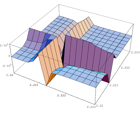
FIG. 2.: The real part of effective potential $\widetilde{\Lambda}(x,x^{\prime})$ at $Z=0.9keV$

It is easy to see that the $n,(\alpha,\alpha)$ effective potential comes to the form close to well-known pseudopotential approach [16], [26]. For example, the task on scattering of particle by system of two heavy centers can be recalled. It is interesting the case of repulsive interactions between the particle and every of both centers with a $\delta$-function form in coordinate space.

It is obvious that two-body subsystem of particle and one heavy center can not form any bound state. However, even in the case the three body system consisting of the particle and two heavy centers will have a bound state [16].

Here we consider a resonator instead of heavy centers system, the simplest resonator being a resonant state of two $\alpha$-particles. And we consider ”the neutron - neutral particle” as a scattering particle. This fact represents a very important point.

It is remarkable that in every of above mentioned cases the scattering particle will be ensnared by subsystem. In case of neutron scattered by the resonator it can be said that the neutron will be in state of total inner reflection between $\alpha$ particles. Lifetime of this three body state will be limited by two $\alpha$-particles subsystem own lifetime.

The resonance state of three $\alpha$-particles can be assumed in this model as more complex resonator.

It should be noted that pseudopotential of scatterring particle by system of few heavy centers leads to the bound states too, i.e. a discrete spectrum can exist in similar systems [16]. Thus, it is additional argument to suggest that the system consisted of few $\alpha$-particles and one neutron has a very reach spectrum.

Calculations have been carried out and give the following results.

In case of $E>0$ calculations confirm an existence of narrow resonance set at very low energies. The amplitude $\overline{P}_{L=0;i,i}$ from (16), with $\Lambda^{eff}_{L=0;i,i}=\overline{\Lambda}_{L=0}(x,x^{\prime})$, have been determined for point set of $x_{0}$ as above.

Figure 3 shows the curve of real part of $\overline{P}_{L=0;i,i}$ in energy region $1.5\div 3\ keV$.

FIG. 3.: The real parts $\overline{P}_{0;i,i}(x,x^{\prime})$ in region $Z>0$, $x=x^{\prime}=0.06$

In case of $Z<0$, i.e. in the region of discrete spectrum, $n(\alpha,\alpha)^{*}$-system has the bound state with very small energy $E_{B}\simeq-4.62\ keV$.

It is very interesting fact that in accordance with results of well-known problem for a particle scattering by two heavy centers (see, above). It is clear that lifetime of this bound state is limited by the own lifetime of $\alpha,\alpha$-resonance.

IV Remarks on astrophysical aspects

It seems there are two serious things which can prevent the resonance fusion: Coulomb forces and nuclear reactions of neutron capture by few $\alpha$-particles subsystem.

Our calculations carried out with Coulomb force between two $\alpha$-particles have confirmed the fact of resonance phenomenon in this case just as the resonance level shifts.

We are going to continue calculations using more precise numerical methods.

As for nuclear reactions of neutron capture a situation is not clear in few body dynamics at very low energies. First of all it is interesting to study a neutron capture directly by few $\alpha$-particle subsystem. We know that one $\alpha$-particle can not capture a neutron.

Introduce $N_{f}$ - average of fusion acts stimulated by neutron in $\alpha$-particle matter. We assume that main part of time between two fusion acts has to be taken by neutron slowing in matter.

Remind that a lifetime of free neutron $\sim 10^{3}$ s, which is infinity in comparison with average time of nuclear fusion, average time of neutron slowing, or lifetime of $\alpha,\alpha$-resonance. Therefore, we can give a rough estimation for $N_{f}$ as ratio between probabilities of $\alpha$-particles fusion and neutron capture: $N_{f}=W_{\alpha}/W_{n}$.

Following a qualitative reasoning we can quess that probability of neutron capture by system of few $\alpha$-particles has to be more less than probability of direct fusion in few $\alpha$-particles subsystem. In last case the neutron becomes free: this is a result from a considerable profit of energy. Moreover, when happened a fusion the few-body system is easy to throw neutron out as the lightest particle than more heavy $\alpha$-particles.

In any case we can talk over the resonance fusion phenomenon. If resonant reactions are effective in stellar matter they present us a possibility to explain a periodic activity of stars, in particular periodic local explosions at the Sun.

As for a problem of free neutrons in stellar matter we can remind about reactions with lightest nuclei, like $d+d\rightarrow^{3}He+n+Q$ and $d+T\rightarrow\alpha+n+Q$, etc. Thus, an existence of free neutrons inside the Sun is possible.

Then, assuming that the small part of the Sun energy is a result of resonance fusion we can understand the problem of little neutrino deficiency incoming to the Earth from the Sun.

It is clear that a lot of interesting effects and phenomena arise from the resonance fusion. Note that the resonance fusion can be easily put into practice to generate energy.

Next article will concern new application projects of resonance fusion.

V conclusions

In conclusion we summerise our results.

The $n,\alpha,\alpha$-system has a set of narrow resonances in low energy region. Their lifetime is comparable to ground $\alpha,\alpha$-resonance.

Interacting with a free neutron the $\alpha,\alpha$-system can act like the resonator. And the $n,(\alpha,\alpha)^{*}$ effective potential has the form close to well-known pseudopotential which describes the scattering of particle by repulsive $\delta$-function forces of two heavy centers. As it is known this pseudopotential gives a bound state of this three-body system.

So, we can say about the new type of fusion - resonance fusion. The neutron can play a role of catalyst to stimulate $\alpha$-particles fusion.

The number of fusion acts stimulated by one neutron may reach large values because of neutron huge lifetime $\sim 10^{3}\ s$ in comparison with nuclear interaction times. By realizing possibility of light nuclei generation in resonance fusion, we can give new answers to questions of origin of light nuclei.

The resonant behavior of reactions may explain periodic activity of stars and periodic local explosions at the Sun. Since it means resonant dependence of energy production on local temperature inside the Sun.

Processes of resonance fusion can be investigated experimentally even nowadays. One of existing and operating installations could be used for.

REFERENCES

- [1] F. Hoyle, Rev. Mod. Phys., 29, 547 (1957).
- [2] W. Fowler: ”Cosmology, Fusion and other Matters”, Associated University Press, 1972.
- [3] V. Bednyakov, Physics of particle and nuclei, 33, 915 (2002).
- [4] G. Streigman, Carnegie Observatories Astrophysics Series, Cambridge Univ. Press., 2 (2003).
- [5] N. Takibayev: in Few-Body Problems in Physics, The XIX European Conference on Few-Body Problems in Physics, Groningen, The Netherlands, 23-27 August 2004, Editors N/ Kalantar-Nayestantki, R. Timmermans and B. Bakker, AIP Conference Proceedings, 768, 349, 2005
- [6] N. Takibayev: in ”Selected topics in theoretical physics and astrophysics: Collection of papers deducated to Vladimir Belyaev on the occasion of his 70th birthday”, Dubna, JINR, 66, 2003
- [7] F.M. Pen’kov, N. Takibayev, Yad. Fiz., 57, 1300 (1994) [Phys. of Atomic Nuclei, 57, 1232 (1994)]
- [8] F.Ajzenberg-Selone, Nuclear Physics, A490, 1 (1988).
- [9] F.Ajzenberg-Selone, Nuclear Physics, A506, 1 (1990).
- [10] S.S. Gernshtein, Yu. V. Petrov, L.I. Ponomarev, Uspekhi Fizicheskikh Nauk, 160, 158 (1990)
- [11] L.D.Blokhintsev, V.I. Kukulin, Yad. Fiz., 53, 693 (1991)
- [12] L.D. Faddeev: ”Mathematical Aspects of the Three Body Problem in Quantum Scattering Theory”, Davey, New York, 1965.
- [13] W. Glockle: ”The Quantum Mechanical Few-Body Problem”, Springer-Verlag, 1983.
- [14] L.D.Blokhintsev, V.I. Kukulin, and D.A. Savin, Yad. Fiz., 51, 1286 (1990)
- [15] R.A. Arndt, D.D. Long, and L.D. Roper, Nucl. Phys., A209, 429 (1973)
- [16] A.I. Baz’, Ya.B. Zel’dovich, and A.M. Perelomov: ”Scattering, reactions, and decays in nonrelativistic quantum mechanics”, Israel Program of Sci. Transl., Jerusalem, 1966
- [17] N. Takibayev, Physics of Atomic Nuclei, 68, 1147 (2005).
- [18] L.D. Faddeev, S.P. Merkur’ev: ”Quantum scattering theory for several particles systems”, Doderecht: Kluwer Academic Publishers, 1993
- [19] M.L. Goldberger, K.M. Watson: ”Collision Theory”, Wiley, New York 1964.
- [20] N. Takibayev, Vestnik KazNPU, Almaty, 2, 47 (2004).
- [21] V.B. Belyaev, ”Lectures on the theory of few-body systems”, Springer-Verlag, Heidelberg, 1990
- [22] E.W. Schmid, H. Ziegelmann: ”The Quantum Mechanical Three-Body Problem”, Pergamon Press, Oxford, 1974
- [23] W. Sandhas: in Few-Body Nuclear Physics, ed. by G. Pisent, V. Vanzani, L. Fonda (IAEA, Vienna 1978), p 1.
- [24] N. Takibayev, F. Pen’kov, Yad. Fiz., 50, 373 (1989)
- [25] N. Takibayev, Physics of Atomic Nuclei, 63, 574 (2000)
- [26] Yu. N. Demkov, JETP 49, 885 (1965)