Direct reconstruction of the quintessence potential
Abstract
We describe an algorithm which directly determines the quintessence potential from observational data, without using an equation of state parametrisation. The strategy is to numerically determine observational quantities as a function of the expansion coefficients of the quintessence potential, which are then constrained using a likelihood approach. We further impose a model selection criterion, the Bayesian Information Criterion, to determine the appropriate level of the potential expansion. In addition to the potential parameters, the present-day quintessence field velocity is kept as a free parameter. Our investigation contains unusual model types, including a scalar field moving on a flat potential, or in an uphill direction, and is general enough to permit oscillating quintessence field models. We apply our method to the ‘gold’ Type Ia supernovae sample of Riess et al. (2004), confirming the pure cosmological constant model as the best description of current supernovae luminosity–redshift data. Our method is optimal for extracting quintessence parameters from future data.
pacs:
98.80.-k astro-ph/0506696I Introduction
Quintessence, a scalar field slowly rolling on its potential, remains one of the most attractive possibilities for explaining the observed acceleration of the Universe (for reviews, see Ref. reviews ). A key goal for future observational programs is to seek definitive evidence for variation in the dark energy density with redshift, which would exclude a cosmological constant. In that event, one would then seek an optimal determination of dark energy properties in the hope of relating them to fundamental physics.
In this paper we assume from the outset that single-field quintessence remains a viable description of observational data, i.e. that it has successfully passed tests against other dark energy paradigms. Our aim is then to obtain optimal constraints on the quintessence potential. We do this by passing directly between the quintessence potential and the observable quantities, focusing in this paper on the luminosity–redshift relation of type Ia supernovae (SNIa). We parametrise the potential, and then constrain those parameters, along with global properties of the Universe, via a likelihood analysis. Additionally, we use model selection criteria in order to select the preferred level of parametrisation of the potential.
Although a variant on the general scheme of reconstruction, our approach is distinct from those already in the literature rec in that we do not rely on a parametrisation of the dark energy equation of state, which then must be related to the dark energy potential via relations which may be approximate (see Guo et al. GOZ for relations in some particular cases). The work closest in spirit to our own is that of Simon et al. simon , who consider an extremely general action and expand the quintessence potential in Chebyshev polynomials (in the redshift range of available data). They relate the expansion coefficients to the redshift evolution of the matter density and Hubble parameter. Those quantities are then extracted from observations and processed into constraints on the potential, those constraints however being as a function of redshift rather than scalar field value. Their treatment is roughly analogous to the inflationary reconstruction method whereby observables such as the spectral index and tensor amplitude are obtained from data, and then related to the inflationary potential via the slow-roll approximation CKLL . Our present paper is analogous to the direct inflaton potential reconstruction method proposed by Grivell and Liddle GL , where the observed power spectra are predicted numerically directly from the inflation potential.
II Formalism
Our set-up is relatively straightforward. We assume that the quintessence field has a potential , which we expand as a power series
| (1) |
where the field is measured in Planck units and (without loss of generality) we take to be presently zero. Note that when we fit these parameters, even in the case of “complete” data we do not necessarily obtain the MacLaurin expansion of the true potential to the same order as this is generally not the best polynomial fit over an interval (in the least-squares or minimax sense). We choose not to use a Chebyshev series as in Ref. simon for the following reasons. Firstly, when fitting, the coefficients of a Chebyshev series would just be linear combinations of the coefficients of a monomial basis polynomial of the same order, so the fits are the same. Furthermore, Chebyshev polynomials would depend on the range takes which in turn depends on the model parameters. Lastly, because we do not fit the potential expansion directly, but rather through a function depending on an integral of the potential, expanding the potential in orthogonal polynomials will not guarantee uncorrelated coefficients.
The scalar field obeys the equation
| (2) |
with the Hubble parameter given by the Friedmann equation
| (3) |
Here is the matter density and the quintessence density. We assume spatial flatness throughout, though the generalisation to the non-flat case would be straightforward. Since then we have the initial condition
| (4) |
We allow to take either sign but results are symmetric under simultaneous reversal of its sign and of odd-order expansion coefficients.
In this article we focus on SNIa data, and hence the observational quantity we need to predict is the luminosity distance as a function of redshift. The luminosity distance is given by
| (5) |
where
| (6) |
is the Hubble-constant-free luminosity distance (for the low redshifts we consider there is no contribution from radiation), and
| (7) |
is the parameter vector describing the model, and
| (8) |
is the quintessence equation of state. The apparent magnitude of a type Ia supernova can be expressed as
| (9) |
where is the absolute magnitude of SNIa (supposing they are standard candles). The distance modulus is defined as
| (10) |
In the following, we should in principle keep as a free parameter. To this end, we define our “observational” quantity to be
| (11) |
where is a measurement of (with the projection of the parameters of the “true” model of the Universe onto our model and its parameter space). Supernovae observations measure , but typically report a distance modulus
| (12) |
where is some estimate of the absolute magnitude. The relevant quantity for fits is thus
| (13) |
where
| (14) |
and . Because of the perfect degeneracy between and , and the fact that the equations are otherwise independent of these parameters, our effective -dimensional parameter vector is
| (15) |
Recall that and determine the matter density through Eq. (4).
To end this section, we note that our formalism includes some possibilities which are not commonly considered. Even if the potential is truncated as a constant, the present field velocity remains a free parameter and so the scalar field can move on this flat potential.111This situation is equivalent to having a pure cosmological constant plus a stiff fluid with . To regain the cosmological constant case we must make the additional assumption that this velocity is zero. Further, the field may be rolling uphill; this may seem unlikely but is valid phenomenologically and might occur in models where the field has recently passed beyond a minimum. Our analysis can also generate models where the scalar field has undergone one or more oscillations about a minimum in the recent past.
III Data analysis
III.1 Likelihood analysis
We carry out a likelihood analysis of the models in comparison to the observational data from Riess et al. Riess:2004nr . We use the 157 SNIa of the ‘gold’ sample.
With a prior distribution , the posterior probability of the parameters , given the data set, is given according to Bayes’ theorem by
| (16) |
where
| (17) |
is summed over all data points, and is a normalisation constant, irrelevant for parameter fitting (but as it is the Bayesian evidence, highly relevant for model selection as discussed below). Here and are the observed distance moduli and their standard deviations, the redshift of the observed supernova and the distance modulus predicted for the redshift by our model with parameters .
To estimate parameters we wish to find explicitly as a function of . This is in general non-trivial, and the standard approach is to explore the parameter space in some way and keep a histogram characterizing . We choose to explore the parameter space using an MCMC approach Gilks ; Lewis:2002ah ; Verde:2003ey ; Dunkley:2004sv . MCMC calculations are generally preferable over grid methods as they scale approximately linearly with the dimension of the problem, rather than exponentially.
Our MCMC algorithm is the following, and makes use of relatively standard step optimisation and convergence/mixing testing.
1. The starting points for the Markov chains are chosen to be close to the expected high-likelihood region with some random spread, checking that they satisfy the priors.
2. Starting with an initial best guess for the covariance matrix of the underlying distribution, we optimise the step sizes of the Gaussian trial distribution with the iteration rule Gilks
| (18) |
where is the estimate of the covariance matrix of the trial distribution, is the number of parameters and the covariance matrix of the chain produced (with our initial best guess). We use chains of 10 000 elements for the optimisation process, and continue updating the trial distribution until there is no significant increase in the sampling efficiency (assessed by comparing the eigenvalues of the covariance matrices). Between each iteration, the parameter space is rotated to the eigenspace of the new covariance matrix, to maximise the efficiency in exploring the shape of the likelihood distribution.
3. The full production run is started. A set of chains with elements each is generated, and only these are used for the final analysis. We generate well separated starting points as before for each of the chains. The chains are tested for convergence and mixing using the Gelman–Rubin test GelmanRubin ; Gilks , which compares the variances within a chain to the variances between chains, which in the asymptotic limit should give a Gelman–Rubin ratio . We require for each parameter. A consistently high and non-convergent Gelman–Rubin ratio is indicative of a very loosely constrained parameter.
In the above, all calculations of covariances and means are done by first dropping an initial burn-in section from the chain. We define the burn-in section following Tegmark et al. Tegmark:2003ud as the elements in the chain from the beginning up to the first element to have a likelihood value above the median likelihood value of the whole chain. The chains were analysed using a slightly modified version of GetDist provided with CosmoMC Lewis:2002ah (again with burn-in sections excluded).
We impose two important constraints on the behaviour of the cosmology within the redshift range , and hence as priors on the parameters. Firstly, the total energy density of the universe must remain positive at all times to exclude collapsing epochs, and secondly we need to avoid models where the kinetic energy would dominate at early epochs (such domination is permitted by the SNIa data alone, but is inconsistent with other data as discussed later). We limit the kinetic contribution to for — see Section IV.3. Most marginalised posterior likelihoods are fairly insensitive to the particular choice of upper limit. However, some marginalised posteriors involving do change significantly. This will be discussed further in the Results section. Additionally we naturally impose . No other priors (e.g. on ) were found to be necessary to obtain acceptable cosmologies.
III.2 Model selection
The order of the power series of the potential can be freely chosen, and the results obtained will obviously depend on the order to which it is taken, with parameters becoming less and less constrained as the order increases. In addition to a determination of the best-fitting parameters within a given model, one therefore needs to compare the different models (i.e. expansions to different orders) in order to determine which is the preferred fit to the data.
Since models with more parameters will always lead to an improved best-fit model, one must use model selection statistics jeff ; mackay ; Lid . These set up a tension between the number of model parameters and the goodness of fit. In the context of Bayesian inference the best such statistic is the Bayesian evidence jeff ; mackay ; for an application to SNIa data see Ref. SWB . The evidence is however difficult to calculate, and in this paper we use a simpler statistic, the Bayesian Information Criterion (BIC) Schwarz ; Lid , which gives a crude approximation to the evidence. The BIC is given by
| (19) |
where is the likelihood of the best-fitting parameters for that model, the number of model parameters, and the number of datapoints used in the fit. Models are ranked with the lowest value of the BIC indicating the preferred model. A difference of 2 for the BIC is regarded as positive evidence, and of 6 or more as strong evidence, against the model with the larger value jeff ; Muk98 .
It is worth mentioning that although we specifically consider a quintessence scenario, a model selection result favouring more than one potential parameter would indicate a dynamical dark energy component more generally, since for every choice of there exists a corresponding quintessence potential, by virtue of Picard’s existence theorem for ODE’s (demonstrated explicitly in e.g. Ref. Padmanabhan:2004av ).
IV Results
The maximum likelihood value and parameters were estimated using the approach described in the preceding Section. We investigated the cosmological constant case and then cases of one, two and three potential parameters (i.e. polynomial orders zero, one, two). Since solving the necessary ODEs is not computationally intensive, we can generate very long chains. For each scenario, 10 chains each containing 1 000 000 elements were obtained.
IV.1 Parameter estimation
IV.1.1 Cosmological constant ()
IV.1.2 Constant potential with kinetic energy ()
Allowing a non-zero kinetic contribution on a constant potential means our parameter vector is
| (21) |
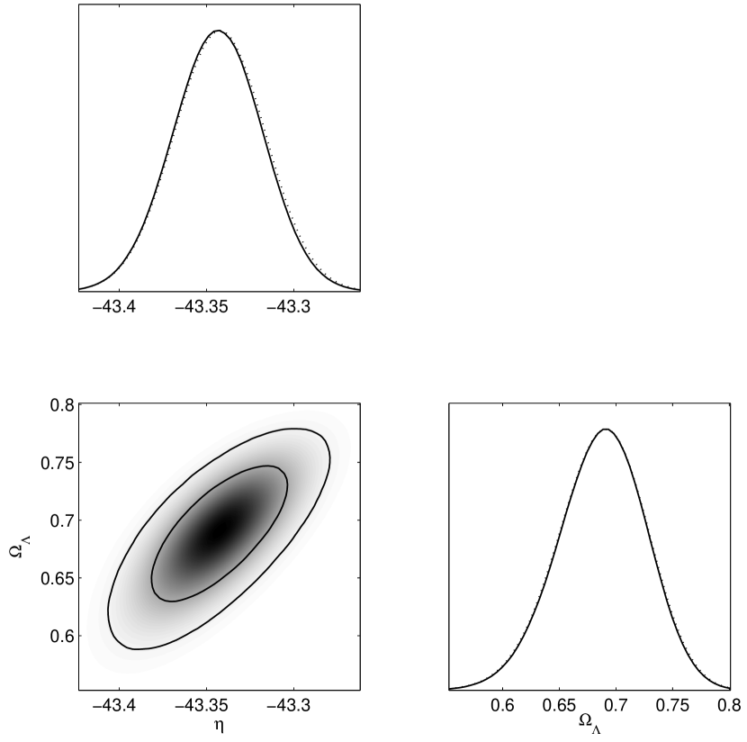
This does, unsurprisingly, improve the fit to data relative to the pure cosmological constant. However, looking at the likelihood distributions in Fig. 3, we clearly see that is not excluded at a statistically-significant level. The bimodality in the distributions is due to the model depending only on .
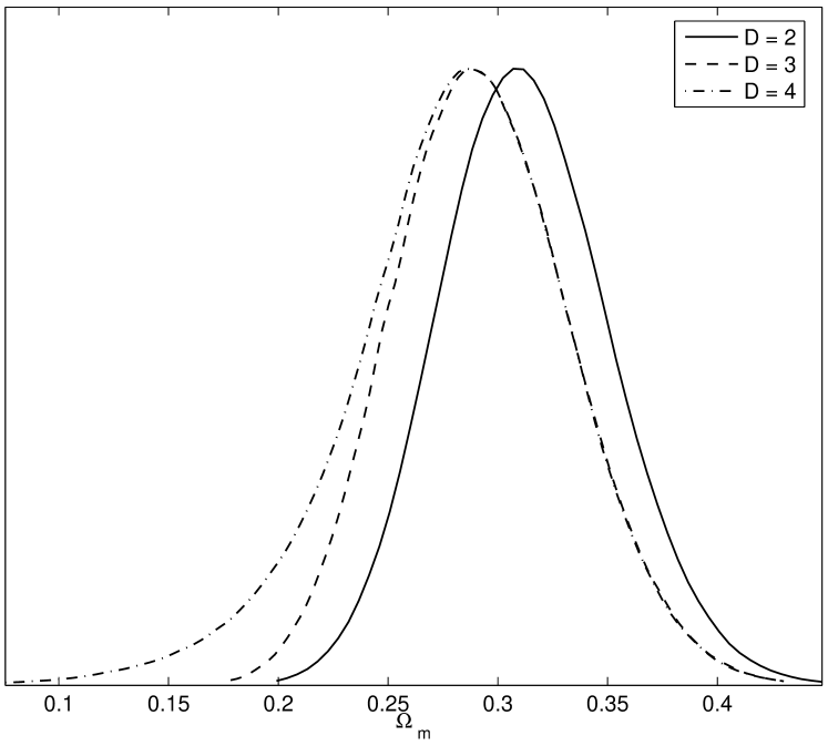
Since a non-zero kinetic contribution is preferred by the data, we also require a higher than in the cosmological constant case. A simple way to see this should be the case is by considering the effective quintessence equation of state: with a kinetic contribution which increases with redshift, the potential term must be larger than for the cosmological constant case to maintain the same effective equation of state at high redshift. The corresponding shift and spread in is shown in Fig. 2.
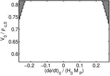
The limits on (and also the other parameters) are dependent on our choice of prior on , but the above conclusions remain even in the (unrealistic) case of no prior. Hence, the choice of prior on can be effectively regarded as a choice of upper limit on . The cut-off of the prior on is illustrated in Fig. 4.
IV.1.3 Linear potential ()
For a linear potential, the parameter vector under consideration is
| (22) |
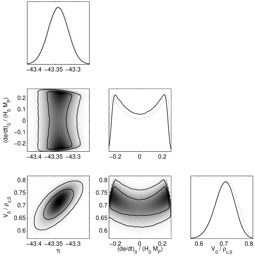
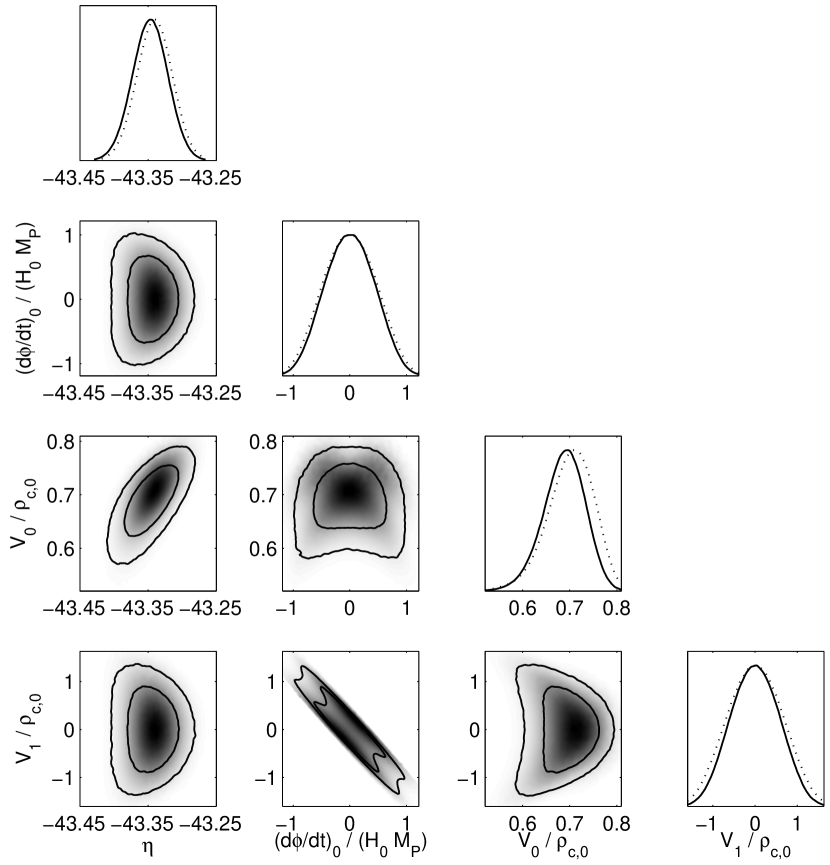
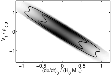
The likelihood distributions (see Fig. 5) show a strong degeneracy between and , which is the main new feature compared to . This is because a particular value of at some earlier redshift can be attained by adjusting either or . Consequently, the best-fit value for is less than for , but with a non-zero .
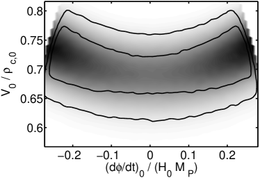
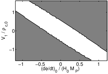
We also note the bimodality in the distribution. This reflects the symmetry under simultaneous change of sign of and odd-order expansion coefficients mentioned in the introduction. Just as for the case , the prior on cuts off the likelihood distribution in a high-likelihood region (see Fig. 6).
An investigation of the linear potential with a different emphasis can be found in Ref. Peri .
| c | ||||
|---|---|---|---|---|
| b | ||||
-
a
The likelihood distribution is an even function of . No confidence limits can be given for , as the prior on cuts in the high-likelihood region and is not excluded at the level. The upper limit on thus corresponds to the maximum allowed value according to our choice of prior on , as discussed in the text, the quoted number being the best-fit.
-
b
The likelihood distribution is symmetric under simultaneous change of sign of and odd-order potential expansion coefficients. No confidence limits can be given for or for the same reason as above.
-
c
Because of the difficulty in obtaining a convergent/well-mixed sampling, as discussed in the text, we choose not to give confidence limits for .
IV.1.4 Quadratic potential ()
The quadratic potential model has the parameter vector
| (23) |
In this case we find that the third potential parameter, , is unconstrained by the data, characterised by a large and oscillating Gelman–Rubin ratio (around 1.3–1.9) for that parameter. Because of that we do not show the likelihoods, since the marginalised distributions will not have the correct weights.
To explore this situation further, we ran additional chains using as our parameter instead of (this corresponds to a change in prior on , since is a function of ). This choice was motivated by the expectation that a cosmological constant, which is achieved in either of the limits or , is very likely to be a good fit, and hence allows us to explore the infinite range in that might be needed. With this choice we get convergent and low Gelman–Rubin ratios, and essentially unconstrained. At we find a small peak in likelihood, but because the distribution remains high and nearly flat outside this peak it is not possible to constrain the parameter without further data.
IV.2 Model comparison
We compare the different models using the BIC, which uses the maximum likelihood achievable by each model. The parameters, likelihoods and BIC values are given in Table 1.
IV.2.1 Cosmological constant ()
The cosmological constant forms the base model for our model comparison, and as is well known provides a good fit to the data. Indeed, the BIC ranks it as preferred to our other models.
 |
 |
 |
 |
|
 |
 |
 |
 |
IV.2.2 Constant potential with kinetic energy ()
As mentioned in the context of parameter fitting, is not excluded at a statistically-significant level. Including this parameter does allow a somewhat better fit to the data, but the BIC penalises its extra parameter leaving the pure cosmological constant model as the preferred description of present data.
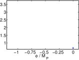
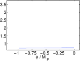
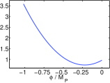
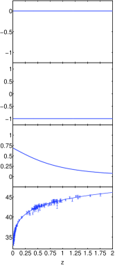
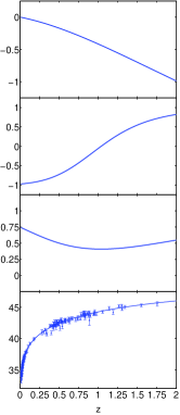
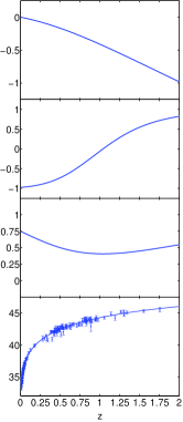
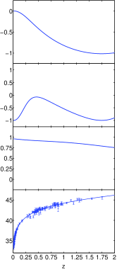
The best-fit cosmology, shown in Fig. 7, exhibits very strong evolution in from kinetic to potential domination over the redshift range of available data. This is not entirely surprising: even a tiny kinetic contribution at present will correspond to a much higher kinetic component at earlier times, as only Hubble friction will work to decrease in this model.
IV.2.3 Linear potential ()
As clearly seen, is well within the preferred region, and so the cosmological constant model is embedded within the allowed parameter space of our extended model. Accordingly, the model comparison of Table 1 prefers the pure cosmological constant model, with the BIC difference arguing quite strongly against the inclusion of the two extra parameters.
The best-fit cosmology (Fig. 7) is practically indistinguishable from the best-fit for . This arises from the strong degeneracy between and ; it turns out that present data are not discriminating in the orthogonal direction.
Within the context of model comparison, a curious point to note is that a field rolling on a linear potential is quite strongly disfavoured as compared to a field rolling on a constant potential (Table 1). This is because the inclusion of a potential slope hardly improves the best-fit at all, while costing an extra parameter. This may seem quite artificial, but is the conclusion of our phenomenological approach. One should note however that the BIC comparison addresses only how well the different models fit the data at hand; when interpretting as a model probability one should bear in mind that this conclusion could be overturned if one felt that the prior model probabilities were quite different.
IV.2.4 Quadratic potential ()
As Table 1 shows, the quadratic model is strongly disfavoured by the BIC. Note that although we have not necessarily obtained a convergent distribution, we can assess the model as the BIC only depends on the maximum likelihood value. However, with such a broad distribution the BIC is expected to be a poor approximation to the Bayesian evidence.
A significant feature of the quadratic potential model is that the best-fit has , see Fig. 7. This is of course in stark contradiction with many other datasets. The evolution of is quite different from that for and , with the field starting high up on the potential, rolling past the minimum and reaching the turning point by the present time. However the preferred parameter region includes models with much more reasonable .
IV.3 Choice of prior on
As mentioned above, we limit the kinetic contribution at . This is necessary because the SNIa data alone favourthe kinetic energy to dominate at , and by inference to be completely dominant at higher redshifts. This is in contradiction to almost any other cosmological dataset (for instance, the mere existence of high-redshift galaxies, and of the cosmic microwave background), and so external priors are necessary to keep us in the physical regime.
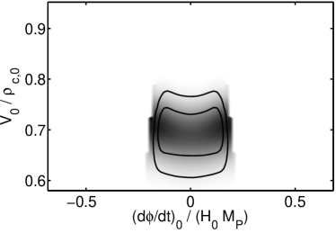
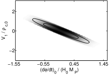
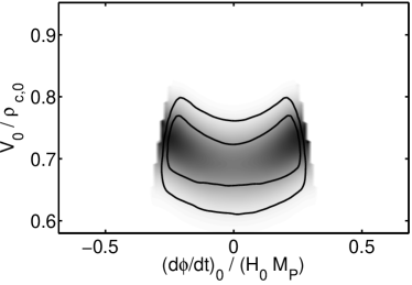
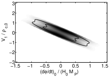
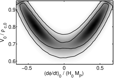
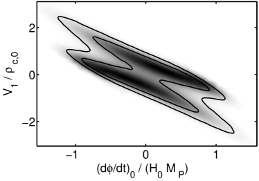
The precise choice of this upper limit on is somewhat arbitrary, and does have a non-negligible impact on the posterior distribution. In terms of marginalised distributions, the distributions involving show the strongest dependence, see Fig. 8. Looking at parameter estimation, as mentioned above the main impact is broader confidence limits. For our model selection analysis, conclusions remain unchanged as the cosmological constant model is still the preferred model even without a prior on for all cases.
V Conclusions
We have described and implemented a reconstruction scheme for quintessence potentials from data, using an MCMC likelihood approach, which we applied to SNIa data. Additionally, we describe the application of model selection using the Bayesian Information Criterion, and point out the generality of any positive evidence found for dynamical dark energy in this approach.
As might be expected, the data provides positive evidence in favour of a cosmological constant in our setup, based on model selection by the BIC. A similar conclusion was previously reached by Saini et al. SWB and by Bassett et al. BCK amongst a set of models parametrised by different equation of state evolution. Some of our distributions do however exhibit broad non-Gaussian regions, which merits a more detailed model selection investigation using the full Bayesian evidence (since the BIC is only a reasonable approximation for sharply-peaked unimodal distributions).
The low-dimensional models are quite well constrained by current data. However, we find that if one allows power series of order two or higher, the parameters (including the linear one) become unconstrained by current SNIa data given our very loose priors. This agrees with what is suggested by the analysis by Maor and Brustein Maor:2002rd in the context of distinguishing potential classes.
We plan to extend this work in several directions. As mentioned above, it would be interesting to extend the model selection to use the full Bayesian evidence, though it will then be essential to consider the issue of prior parameter ranges, which the BIC sidesteps. Generalisation to include further cosmological datasets is desirable, especially CMB anisotropies, though that will require the potential expansion to be valid over a much wider range of redshifts. Finally, it would be interesting to explore whether in the context of tracking models it might be possible to eliminate the parameter , which ought to be determined via an early tracking regime.
Acknowledgements.
M.S. was supported at Sussex by a Marie Curie Fellowship of the European Community programme HUMAN POTENTIAL under contract HPMT-CT-2000-00096. A.R.L. and D.P. were supported by PPARC. We thank María Beltrán, Pier Stefano Corasaniti, Irit Maor, Claudia Quercellini and Erandy Ramirez for helpful discussions, and Jon Urrestilla for computer assistance. We additionally acknowledge use of the UK National Cosmology Supercomputer funded by Silicon Graphics, Intel, HEFCE and PPARC.References
- (1) V. Sahni and A. Starobinsky, Int. J. Mod. Phys. D9, 373 (2000), astro-ph/9904398; T. Padmanabhan, Phys. Rept. 380, 235 (2003), hep-th/0212290.
- (2) D. Huterer and M. S. Turner, Phys. Rev. D60,081301 (1999), astro-ph/9808133; A. A. Starobinsky,JETP Lett. 68, 757 (1998)[Pisma Zh. Eksp. Teor. Fiz. 68, 721 (1998)], astro-ph/9810431; T. Nakamura and T. Chiba, Mon. Not. Roy. Astron. Soc. 306, 696 (1999), astro-ph/9810447; B. F. Gerke and G. Efstathiou, Mon. Not. Roy. Astron. Soc. 335, 33 (2002), astro-ph/0201336; C. Wetterich, Phys. Lett. B594, 17 (2004), astro-ph/0403289.
- (3) Z.-K. Guo, N. Ohta and Y.-Z. Zhang, astro-ph/0505253.
- (4) J. Simon, L. Verde and R. Jiminez, Phys. Rev. D71, 123001 (2005), astro-ph/0412269.
- (5) E. J. Copeland, E. W. Kolb, A. R. Liddle and J. E. Lidsey, Phys. Rev. D48, 2529 (1993), hep-ph/9303288.
- (6) I. J. Grivell and A. R. Liddle, Phys. Rev. D61, 081301 (2000), astro-ph/9906327.
- (7) A. G. Riess et al. [Supernova Search Team Collaboration], Astrophys. J. 607, 665 (2004), astro-ph/0402512.
- (8) L. Verde et al., Astrophys. J. Suppl. 148, 195 (2003), astro-ph/0302218.
- (9) J. Dunkley, M. Bucher, P. G. Ferreira, K. Moodley and C. Skordis, Mon. Not. Roy. Astron. Soc. 356, 925 (2005), astro-ph/0405462.
- (10) A. Lewis and S. Bridle, Phys. Rev. D 66, 103511 (2002), astro-ph/0205436.
- (11) W. R. Gilks, S. Richardson, and D. J. Spiegelhalter (eds.), Markov Chain Monte Carlo in Practice, Chapman & Hall (1996).
- (12) A. Gelman and D. Rubin, Statistical Science 7, 457 (1992).
- (13) M. Tegmark et al. [SDSS Collaboration], Phys. Rev. D69, 103501 (2004),astro-ph/0310723.
- (14) H. Jeffreys, Theory of Probability, 3rd ed, Oxford University Press (1961).
- (15) D. J. C. MacKay, Information theory, inference and learning algorithms, Cambridge University Press (2003).
- (16) A. R. Liddle, Mon. Not. Roy. Astron. Soc. 351, L49 (2004), astro-ph/0401198.
- (17) T. D. Saini, J. Weller and S. L. Bridle, Mon. Not. Roy. Astron. Soc. 348, 603 (2004), astro-ph/0305526.
- (18) G. Schwarz, Annals of Statistics 5, 461 (1978).
- (19) S. Mukherjee, E. D. Feigelson, G. J. Babu, F. Murtagh, C. Fraley, and A. Raftery, Astrophys. J. 508, 314 (1998), astro-ph/9802085.
- (20) T. Padmanabhan, Curr. Sci. 88, 1057 (2005), astro-ph/0411044.
- (21) L. Perivolaropoulos, Phys. Rev. D71, 063503 (2005), astro-ph/0412308.
- (22) B. A. Bassett, P. S. Corasaniti, and M. Kunz, Astrophys. J. Lett. 617, L1 (2004), astro-ph/0407364.
- (23) I. Maor and R. Brustein, Phys. Rev. D67, 103508 (2003), hep-ph/0209203.