SALT: a Spectral Adaptive Light curve Template for Type Ia Supernovae

We present a new method to parameterize Type Ia Supernovae (SN Ia) multi-color light curves. The method was developed in order to analyze the large number of SN Ia multi-color light curves measured in current high-redshift projects. The technique is based on empirically modeling SN Ia luminosity variations as a function of phase, wavelength, a shape parameter, and a color parameter. The model is trained with a sample of well-measured nearby SN Ia and then tested with an independent set of supernovae by building an optimal luminosity distance estimator that combines the supernova rest-frame luminosity, shape parameter, and color reconstructed with the model. The distances we measure using $B$- and $V$-band data show a dispersion around the Hubble line comparable or lower than obtained with other methods. With this model, we are able to measure distances using $U$- and $B$-band data with a dispersion of $0.16\pm 0.05$ around the Hubble line.

1 Introduction

Type Ia supernovae (SNe Ia) are a powerful tool for studying the evolution of the luminosity distance as a function of redshift and for subsequently constraining the cosmological parameters. SNe Ia are indeed very luminous and “standardizable” candles, and have lead to the discovery of the acceleration of the Universe (Riess et al. 1998; Perlmutter et al. 1999).

Although often described as a homogeneous class of objects, SNe Ia exhibit variability in light curve shapes, colors, intrinsic luminosity, and spectral features. Finding correlations among SN Ia observables is motivated by improving the estimation of their intrinsic luminosity on an event-by-event basis, in order to reduce the scatter in luminosity distance estimates. The main correlations observed in photometric measurements are:

• a width-luminosity (or brighter-slower) relation, which expresses the fact that brighter supernovae have a slower decline rate than fainter ones (Pskovskii 1977; Phillips 1993; Riess et al. 1995; Hamuy et al. 1996b; Perlmutter et al. 1997).

• a brighter-bluer relation, which was made explicit in Tripp (1998); Tripp & Branch (1999); Parodi et al. (2000), and assumed to be due to extinction by dust in other works (Riess et al. 1996a, 1998; Perlmutter et al. 1999; Tonry et al. 2003; Knop et al. 2003; Barris et al. 2004).

The case of the brighter-bluer relation is interesting. Even if authors fully agree neither on the origin of the effect nor on the strength of the correlation, most, if not all, recent attempts to build a SN Ia Hubble diagram have made use of color in their distance estimator. Riess et al. (1996b) summarizes previous work on the subject and proposes a way to reconcile divergent interpretations of data by taking into account the correlation between light curve shape and color. New methods using color information have also been recently proposed to estimate luminosity distances (see for example Wang et al. 2003 and Wang et al. 2005). We will bring to the debate our own estimations of the correlation strength and its wavelength dependence.

Cosmological measurements using SNe Ia are based on comparing nearby and distant objects. In order to reduce the sources of systematic uncertainties, it is important that all distances are derived using the same procedure, especially when considering large samples such as those being collected by the ESSENCE or SNLS projects. To analyze these data sets, the following constraints have to be taken into account:

• High redshift objects often lack late-time photometric data (or have one of too poor quality) which makes it impracticable to estimate color from late-time data as proposed by Lira et al. (1998).

• Above redshifts $z\sim 0.8$, rest-frame $U$-band measurements have to be used because of the limitation of silicon detectors. Incorporating rest-frame $U$-band measurements on the same footing as the commonly used rest-frame $B$- and $V$-band data is hence highly desirable.

• Applying cuts on light curve parameters should be prohibited since the resolution on these parameters follows the photometric resolutions and hence degrades with redshift, therefore biasing the event sample. In particular, cuts on colors to eliminate reddened events are to be avoided.

Various techniques have been used to estimates distances. Phillips (1993) and Perlmutter et al. (1997) fit one band at a time, and derive distances from light curve parameters measured in different bands (usually $B$ and $V$ bands), sometimes relying on late time measurements to measure host galaxy extinction. A recent and refined version of this approach can be found in Wang et al. (2005), and in Wang et al. (2003) it is proposed to fit $B-V$ as a function of $B$. These methods do not make use of rest-frame $U$-band measurements. Nugent et al. (2002) discuss in detail the problems associated with SN Ia $U$-band photometry. They mention in particular the apparent large intrinsic variations of the UV luminosity among similar supernovae as well as our lack of understanding of the SN Ia UV photometry –principally due the uncertainties which affect the large extinction corrections which have to be applied to the data. Nevertheless, it is important to try and incorporate rest-frame $U$-band data to estimate distances.

An extension of Perlmutter et al. (1997) to rest-frame $U$-band data was developed in Knop et al. (2003), but at the expense of adding a large distance systematic (and probably statistical) uncertainty. Similarly, the MLCS method (Riess et al. 1995, 1996a) has been extended to include $U$-band measurements under the name of MLCS2k2 (Jha 2002) and used in Riess et al. (2004), but also at the expense of a worsened distance resolution (Jha 2002). We will show that our model predicts light curves for any band located between rest-frame $U$ and $R$ bands and that we are able to get a similar or better distance resolution with both rest-frame ($B,V$) and ($U,B$) band pairs.

We propose here to parameterize the light curve model with a minimal parameter set: a luminosity parameter, a decline rate parameter and a single color parameter. Our approach will be to build a phenomenological model of the expected SN flux, continuously varying with phase, wavelength, decline rate and color, in order to capture all these features at once. This approach offers several practical advantages which make it easily applicable to high-redshift SNe Ia currently measured in large projects. First, the k-corrections are built into the model and not applied to the data. This allows one to propagate all the uncertainties directly from the measurement errors. More importantly, when needed, we make use of the SN rest-frame $U$-band fluxes to estimate the supernova distances.

In Sect. 2 we describe the semi-analytic model used. We then describe, in Sect. 3, how the coefficients of the model are determined by an iterative training based on a set of well-sampled nearby SNe Ia taken from the literature. We also highlight some properties of the resulting model. At this stage, the aim is to model multi-color light curves and not to estimate luminosity distances. The model is tested in Sect. 4 with an independent set of SNe Ia in the Hubble flow. A luminosity distance estimate is then constructed from the fitted parameters of the light curve model. It is used to build Hubble diagrams successively from $(B,V)$ and $(U,B)$ light curve pairs. In order to assess the precision of this approach, we compare distance estimates of the same events obtained from the $(U,B)$ and $(B,V)$ band pairs and with other distance estimators.

2 The light curve model

2.1 Model definitions

As already mentioned, we choose to parameterize light curves (more precisely light curve pairs or light curve triplets when available) using a single luminosity, a single shape parameter and a single color. The choice among possible implementations is largely arbitrary. We choose the following parameters, which enable comparisons to be made with previous works:

• ${\bf f_{0}}$ : a global intensity parameter which varies with redshift like the inverse of the luminosity distance squared,

• ${\bf s}$ : a time stretch factor as the decline rate indicator (Perlmutter et al. 1997). In Goldhaber et al. (2001), this parameter is shown to apply to the rising part of the light curve as well. However, while the stretch paradigm describes well the bright part of the $B$ light curve, it does poorly at late time. It also fails to capture the shape variations in the other bands. This is why our model uses the stretch parameter as an index rather than the stretch paradigm itself. As described below, by construction our model follows exactly the stretch paradigm in the $B$ band.

• ${\bf c}$ = $(B-V)_{max}+0.057$, where $(B-V)_{max}$ is measured at B maximum, and $-0.057$ is the chosen reference color (Vega magnitudes) of a SN Ia.

• $t_{max}^{B}$ : the date of maximum in the rest-frame $B$ band

With these definitions, the expected counting rate $f_{SN}$ in a given pass-band $T$, of a supernova at redshift $z$, and at a phase $p\equiv(t-t_{max}^{B})/(1+z)$, can be written:

$$f_{SN}(p,z,T)=f_{0}\,(1+z)\int\phi(p,\lambda,s,c)\ \frac{\lambda}{h\,c}\ T(\lambda(1+z))\,d\lambda$$

$\phi(p,\lambda,s,c)$ is a model of the SN Ia energy luminosity per unit wavelength. It may vary with the supernova stretch and color. Note that the potential extinction by dust in the host galaxy is not explicit in the equation. Instead, we choose to incorporate it in the model $\phi(p,\lambda,s,c)$ as discussed below.

Building an average spectral template $\phi$ as a function of phase, wavelength, color and stretch from observations is complicated because of the inhomogeneity and incompleteness of published data. Although some spectral features have been correlated with stretch, we do not have yet a complete knowledge of spectral diversity as a function of phase. In most of the approaches to SN Ia light curve fitting, the limited knowledge of spectral variability impacts on the accuracy of cross-filter k-corrections, defined as expected ratios of fluxes in different bands at the same phase (Kim et al. 1996; Nugent et al. 2002).

In Nugent et al. (2002), it was shown that the variation in k-corrections from one supernova to another depends primarily on the supernova color, and to a lesser extent on spectral features. Hence we neglected the variability of those spectral features in the modeling of light curves.

In order to implement stretch dependent light curve shapes and colors we therefore used the following approximation:

$$f_{SN}(p_{s},z,T)=f_{0}\,(1+z)\int\phi(p_{s},\lambda)\,\frac{\lambda}{h\,c}\,T(\lambda(1+z))\,d\lambda$$

$$\times\ \exp\left[-0.4\,\ln(10)\times{\cal K}(p_{s},\lambda_{T},s,c)\right]$$ (1)

where $p_{s}\equiv p/s$ is a stretch-corrected phase. This functional form defines the light curve model.

In equation 1, $\phi$ no longer depends explicitly on $s$ and $c$, and ${\cal K}(p_{s},\lambda,s,c)$ is a smooth “correction” function of our four variables. $\lambda_{T}$ is the central wavelength of the filter $T$. ${\cal K}$ enables one to implement light curve shape variations that are more complicated than simple dilation of the time scale, along with stretch dependent colors. As described below, ${\cal K}$ varies smoothly with $\lambda$; this justifies placing it outside the integral over wavelength. We also considered keeping ${\cal K}(p_{s},\lambda_{T},s,c)$ inside the integral. It changed the results of the fits by less than 1%, while the computing time was multiplied by a factor of 10.

Equation (1) implements k-corrections for an average SN Ia, conforming to the common practice. The approach proposed here will be easy to adapt when constructing a stretch-dependent spectral template becomes possible.

The k-corrections are usually applied to data. Here, they are incorporated into the model. This offers a few practical advantages: first, light curves can be generated for arbitrary pass-bands (within the spectral coverage of $\phi$ and ${\cal K}$); light curves in the observed pass-bands can be directly fitted to the data. Second, the light curve parameter uncertainties extracted from the fit incorporate all uncertainties propagated from measurement uncertainties; for example, uncertainties introduced in the k-corrections by the possibly poor determination of the date of maximum and/or color are propagated into the parameters uncertainties.

The functions $\phi$ and ${\cal K}$ define the model. Once they are determined, one can fit the supernova photometric data points, measured in a minimum of two pass-bands, to estimate $f_{0}$, $s$, $c$, and a date of $B$ maximum light, which is a nuisance parameter. With only one passband, $c$ must be held fixed.

For $\phi(p_{s},\lambda)$, we use a template spectrum assembled by P. Nugent (Nugent et al. 2002 and private communication) smoothed along the phase (time) axis, and normalized as a function of phase to the $B$-band light curve template “Parab -18” of Goldhaber et al. (2001). Any smooth variation of the template $\phi$ with phase or wavelength is irrelevant at this level, since it may be changed by the function ${\cal K}(p_{s},\lambda,s,c)$. The only important quantities in $\phi(p_{s},\lambda)$ are the SN Ia spectral features, intended to be realistic on average.

The empirical correction function ${\cal K}$ is implemented as a sum of two polynomials:

$${\cal K}(p_{s},\lambda,s,c)={\cal K}_{s}(p_{s},\lambda,s)+{\cal K}_{c}(\lambda,c)$$ (2)

where we explicitly separate the corrections associated with the parameters $s$ and $c$ to clarify their interpretation. ${\cal K}_{s}(p_{s},\lambda,s)$ modifies the shape of light curves and absorbs any stretch–color relation except for the $(B-V)_{max}$ color. Indeed we want $c$ to describe exactly the $(B-V)_{max}$ color. ${\cal K}_{c}(\lambda,c)$ is then a color correction as a function of wavelength and color.

In order to remove all degeneracies among coefficients, the model must fulfill the following constraints:

$${\cal K}_{s}(p_{s}<35,s,\lambda_{B}) = 0$$

$${\cal K}_{s}(p_{s}=0,s,\lambda_{V}) = 0$$

$${\cal K}_{c}(\lambda,c=0)={\cal K}_{c}(\lambda_{B},c) = 0$$

$${\cal K}_{c}(\lambda_{B},c)-{\cal K}_{c}(\lambda_{V},c) = c$$

where $\lambda_{B}$ and $\lambda_{V}$ refer to the mean wavelengths of the B and V filters. The first constraint ensures that the parameter $s$ actually defines the stretch in $B$ band, since the template is not modified for $\lambda=\lambda_{B}$. The remaining constraints define $c$ as the $B-V$ color (relative to the spectral template) at maximum $B$, for all stretches. Note that other colors may (and in fact will) depend on $s$ at fixed $c$. $f_{0}$ describes the actual peak flux in $B$. It is in no way “corrected” for the brighter-slower relation.

${\cal K}_{s}$ is implemented as a polynomial of degree $D_{p}$ in phase, $D_{\lambda}$ in $\lambda$ and $D_{s}$ in stretch respectively. Similarly, ${\cal K}_{c}$ is a polynomial of degree $D_{p}$ in phase and $D_{c}$ in color. In this study, we chose for the degrees of polynomials $(D_{p},D_{\lambda},D_{s},D_{c})=(4,3,1,1)$. The large degree in phase permits a detailed adaptation of the model light curve shapes to the actual data. The other degrees correspond to the minimal number of coefficients (a degree 3 in wavelength is chosen to adapt colors in $UBVR$, independently). The ${\cal K}$ polynomials are then defined by 48 coefficients, but the constraints reduce the number of independent coefficients to 34. There are 32 free coefficients for ${\cal K}_{s}$ and 2 free coefficients for ${\cal K}_{c}$. We will call “training” the determination of these coefficients from measurements of nearby SNe Ia.

2.2 Normalization of transmissions

The value of $f_{0}$ depends on the normalization of the spectral template $\phi$. This is not an issue when comparing nearby and distant supernovae to measure cosmological parameters, since only flux ratios matter: all objects have to be fitted using the same model. For $H_{0}$ measurements, one would need to normalize $(\phi)$ using SNe Ia at known distances, but we will not perform this here.

More important is the apparent dependence of the value of $f_{0}$ with respect to the normalization of the transmission $T$ (equation 1). Since we aim at fitting multi-color light curves, observed with different instruments, with a single set of parameters $(f_{0},s,c)$, it is mandatory to remove this dependence.

All photometric data are expressed in units of the integrated flux $f_{ref}$ (deduced from the zero point) of a known standard spectrum $\phi_{ref}$ (e.g. Vega). While the functional form of $T(\lambda)$ is determined by optical transmission measurements its normalization can be determined from $f_{ref}$ and $\phi_{ref}$ via the relation

$$\int\phi_{ref}(\lambda)\,\frac{\lambda}{h\,c}\,T(\lambda)\,d\lambda\,=\,f_{ref}$$ (3)

The filter transmissions are usually published as series of numbers (as in Bessell 1990), and this leads to ambiguities: for example, Suntzeff et al. (1999) writes ”Note that Bessell (1990) defines the sensitivity function as the product of the quantum efficiency of the detector+telescope, the filter transmission curve, the atmospheric extinction, and a linearly increasing function of wavelength.”. The ambiguity is whether the transmission refers to signal per unit energy, or signal per photon flux. Attributing dimensions to transmissions solves the ambiguity.

There have also been concerns about the relative weights of the different wavelengths in the integrals over wavelength (Nugent et al. 2002), namely whether one should sum photons or energies. If one aims at reproducing the instrument response to an arbitrary spectral energy density, the mathematical integrals should mimic the physical integration process of the instrument (Fukugita et al. 1996). For example, if one considers a CCD-based observing system, the effective transmission $T(\lambda)$ will be proportional to a number of photo-electrons per photon. So one should not integrate photon counts nor energies, but charge on the detector (or ADC counts).

3 Training the model

Since $f_{0}$ describes the observed luminosity in the $B$ band (because of the constraints applied to the corrections), the model only incorporates stretch-shape and stretch-color relations, but no correlation involving luminosity. This option was chosen in order to allow us to train the model with objects at unknown distances, in particular the nearby objects in the sample of Jha (2002) measured in the $U$ band. If one offsets all magnitudes of each training object by an arbitrary amount, possibly different for each object, the resulting model will not change. One could then consider incorporating high redshift objects into the training, but we choose not to do it here.

3.1 The nearby SN Ia Sample

The model was trained and tested using a sample of published nearby supernova light curves. We collected 122 SNe Ia for which $B$- and $V$-band light curves are available in the literature, including data from Hamuy et al. (1996b); Riess et al. (1996b) and Jha (2002) for a total of 94 objects, and 28 additional supernovae collected from various sources (see the caption of table 1).

Objects were then selected based on two main criteria. First, we kept supernovae with at least two measurements before the maximum in the $B$ or the $V$ band. This is necessary to ensure that the date of maximum is well defined and that the measurements can safely be used as a function of phase. Out of the whole sample, 56 SNe satisfied this criterion. Then under-luminous peculiar supernovae: SN 1991bg, SN 1998bp, SN 1998de and SN 1999by (Howell 2001; Li et al. 2001b), and the peculiar objects SN 2000cx and SN 2002er (Li et al. 2001a; Pignata et al. 2004) were rejected from our sample. There are a number of reasons for this choice; the most important one being the spectral difference between normal and SN 1991bg-like SNe Ia. Since our model is built using a spectral template describing the features of the average normal SN Ia, it is not well suited for describing very different objects, such as SN 1991bg-like events. We note that, this is not a constraint for cosmological studies since, so far, no under-luminous SNe have been found in distant SN searches. Furthermore, if present at high-redshift, these objects would easily be identified both from spectroscopy and from their $B-V$ color evolution (see for instance Phillips et al. 1999; Garnavich et al. 2004).

SN 1991T-like events were kept in the sample. This ”sub-class” of over-luminous SNe Ia is spectroscopically identified by the presence of unusually weak absorption lines during the pre-maximum phase. These are more difficult to identify than their under-luminous counterparts in low signal-to-noise spectra, such as those usually available for high redshift SNe. Moreover, the $B-V$ color evolution is not particularly different from the one of normal SNe. Ideally, one should use a different spectral template for fitting this kind of events. We estimate the errors introduced in the k-corrections using a standard SN Ia spectral template to be of a few percent in the worst cases, and well within the final dispersion in the peak luminosity of SNe Ia. We further note that, the uncertainty due to using a non optimal spectral template is analogous to the uncertainty in the cross filter $k$-corrections used in standard methods.

The resulting sample of 50 SNe was then split into two sets: a training sample and a test sample. The training sample was used to adjust the coefficients of the polynomials of the model. It contains all the supernovae with redshifts smaller than 0.015 (not in the Hubble flow) and 6 supernovae at redshifts above 0.015, for which with $U$-band data was available, in order to improve the model in this wavelength region. The training sample contains the 34 supernovae listed in table 1. The test sample contains 26 supernovae (table 2). Note that the two samples are not completely independent. Indeed, they share ten supernovae with $U$-band light curves, since such events are rather scarce.

The data was not pre processed in any way prior to fitting. To account for the Milky Way extinction, we incorporate it into the instrument transmission, using the law from Cardelli et al. (1989) with a color excess $E(B-V)$ obtained from Schlegel et al. (1998) dust maps at the position of the object to fit.

3.2 Training the Model

All the published nearby supernova magnitudes are expressed in the Johnson-Cousins $UBVR$ system. In Equation (1), we use models of the instrument transmissions as a function of wavelength. We adopted the transmission functions published by Bessell (1990), and interpreted them as $\lambda\,T(\lambda)$ (see equation 1), i.e. counts per unit energy, following a footnote of Suntzeff et al. (1999).

Training the model consists in determining the ${\cal K}(p_{s},\lambda,s,c)={\cal K}_{s}(p_{s},\lambda,s)+{\cal K}_{c}(\lambda,c)$ correction function (Eq. 2) using the training sample data in the $UBVR$ bands. The $R$ band was introduced to avoid relying on extrapolation for measurements beyond rest-frame $V$ band. We start with a first guess:

$${\cal K}_{s}(p_{s},\lambda,s) = 0$$

$${\cal K}_{c}(\lambda,c) = c\times(\lambda-\lambda_{B})/(\lambda_{V}-\lambda_{B})$$

and we use an iterative algorithm which can be sketched as follows:

1. Fit the light curves using the current determination of ${\cal K}$.

2. Fit $\delta\,{\cal K}(p_{s},\lambda,s,c)$, an instance of the ${\cal K}$ function, on the light curve residuals. During this step, identify and remove the outliers data points.

3. ${\cal K}\leftarrow{\cal K}+\delta\,{\cal K}$.

4. GOTO step 1, until $\delta\,{\cal K}$ becomes negligible.

All the available data, i.e. the $UBVR$ residuals, up to large phases were used to determine the ${\cal K}$ function (step 2). However, not all the data points were used to fit the light curves (step 1): the $R$-band data was not used and only $UBV$ photometric points with phases ranging from $-15$ days to $+35$ days were used since we are mostly interested in describing the rest-frame $UBV$ central part of the supernova light curves.

3.3 Results of the training

The fit converged after four iterations. 2480 measurement points were fitted, and 39 were discarded as outliers (at the 3 $\sigma$ level). Compared to the number of free coefficients of the model, we can safely conclude that the model is not over-trained. The standard deviations of the residuals to the model in $UBVR$ are respectively of $0.09,0.09,0.06,0.07$ magnitudes. Figure (1) shows the final $U$, $B$, $V$ and $R$ templates obtained at the end of the process as a function of stretch. By construction, the rest-frame $B$ and $V$-band magnitudes at maximum do not vary with stretch. We find a strong dependence of $(U-B)_{max}$ with stretch ($\delta(U-B)_{max}\simeq-\,\delta s$, compatible with Jha 2002), which is an essential feature for the model to reproduce in order to estimate a reliable color in the wavelength range between $U$ and $B$. The model also manages to reproduce a a stretch-dependent secondary shoulder in the $R$ band. We also notice that the $R$-band light curves cross each-other for different values of the stretch. This reproduces well the fact that the brighter slower relation is weaker in the redder pass-bands, as noted by Phillips et al. (1999). The residuals to the light curve fit are shown figure 2.

Figure 1: The $UBVR$ template light curves obtained after the training phase for different values of the stretch and null color. Note the strong variations of the $U$-band maximum with the stretch. Note also the after max shoulders in the $V$ and $R$ bands. The model also reproduces well the fact that the brighter-slower relation is weaker in the $R$ band than in the $B$ or $V$ bands. The model does not incorporate the brighter-slower correlation. The apparent brighter-slower correlation for the $U$ band is, in fact, a stretch-color correlation.

Figure 2: Residuals to the light curve fit as a function of phase, for supernovae from the training sample (open symbols) and the test sample (filled symbols). There is no significant difference between the distributions obtained with both samples which proves that the model is not over-trained. The systematic residuals as a function of phase are a direct consequence of the limited number of parameters (5) used to implement the corrections ${\cal K}_{s}$ as a function of phase. Increasing this number would remove this systematic trend in residuals, but some parameters would be poorly constrained in the $U$ band where photometric data is scarce.

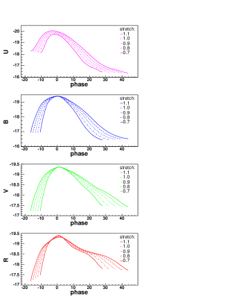
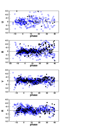
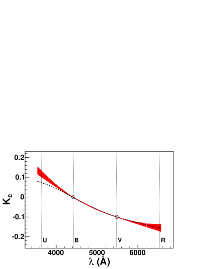
Figure 3 represents the color correction ${\cal K}_{c}(\lambda,c)$ for $c=0.1$ compared to the dust extinction law from Cardelli et al. (1989). Interestingly enough, the law we obtain follows pretty well that of Cardelli in the $R$ band but not in the $U$ band where we get a stronger dependence on $c$. Also shown (shaded area) is the uncertainty on ${\cal K}_{c}$ derived from the $\chi^{2}$ increment (normalized to the number of supernovae) of the fit to the light curve residuals. The Cardelli law in the $U$ band is at 3.7 standard deviation from the best fit value.

As a consequence, we deduce that the relation between E(B-V) and E(V-R) are very similar (i.e. indistinguishable) to the ones expected from reddening by dust. This similarity, noted by Riess et al. (1996b), does not prove however that $c$ can be interpreted as reddening by dust; an additional requirement for this hypothesis to be valid would be that the peak $B$-band magnitude increases with $c$ by a value of $R_{B}\times c$. We will see that this is not the case in the next section. Let us also emphasize that the stretch dependent part of the $U-B$ and $V-R$ colors are included in the stretch dependent term ${\cal K}_{s}(p_{s},\lambda,s)$, and not in the color curve of figure 3.

Figure 3: The color correction ${\cal K}_{c}$ as a function of wavelength for a value of $c$ of 0.1 (thick line). The shaded area corresponds to one standard deviation to the best fit value. The dashed curve represents the extinction with respect to $B$ band, $(A_{\lambda}-A_{B})$, from Cardelli et al. (1989) with $R_{V}=3.1$ and $E(B-V)=0.1$. The curves are compatible in the $R$ band but not in the $U$ band (by construction they match in $B$ and $V$ bands as illustrated with the open circles).

4 Performance study

Once the correction function ${\cal K}(p_{s},\lambda,s,c)$ is determined, we can fit the model on the sample of nearby SN Ia light curves listed in table 2. This allows us to perform various consistency checks, in order to make sure that the model describes well the $UBV$ photometry of SNe Ia.

A first test consists in checking the ability of the model to reproduce the shape and color features of the independent set of SNe Ia. This is demonstrated on figure 2 which shows the residuals to the fits of light curves of SNe from the test sample.

4.1 Distance estimate

The global intensity parameter $f_{0}$ is proportional to $d_{L}(z)^{-2}$ and inversely proportional to the normalization of $\phi$. One can define a rest-frame $B$ magnitude $m^{*}_{B}$ (Perlmutter et al. 1997) which removes this artificial dependence on the model normalization,

$$m^{*}_{B}=-2.5\,\log_{10}\frac{f_{SN}(0,z,T^{*}_{B})}{(1+z)\,f_{ref}(T_{B})}$$ (4)

where $f_{SN}$ and $f_{ref}$ are respectively defined by equations 1 and 3, $T_{B}$ is the transmission of the $B$ filter and
$T^{*}_{B}(\lambda)=T_{B}(\lambda/(1+z))$ is a redshifted $B$ transmission. One can check that $m^{*}_{B}$ varies as $5\log_{10}d_{L}(z)$ with redshift and that $m^{*}_{B}\rightarrow m_{B}$ for $z\ll 1$, where $m_{B}$ is the conventional $B$ magnitude.

We incorporate the Hubble parameter dependence of $d_{L}$ in a constant parameter $M_{B}^{70}=M_{B}-5\,\log_{10}\left(h_{70}\right)$, which is the average absolute magnitude of a SN Ia with $s=1$ and $c=0$, for a value of the Hubble parameter of 70 km.s^-1.Mpc^-1.

As mentioned in the introduction, the peak luminosity of SNe Ia is correlated to stretch and color, so we may build a distance estimator that accounts for those correlations and as a result reduces the dispersion. Following Tripp (1998), we adopt linear corrections of coefficients $\alpha$ and $\beta$ respectively for stretch and color. The distance estimator is then

$$m^{*}_{B}-M_{B}^{70}-43.16+\alpha\,(s-1)-\beta\,c$$ (5)

Its expectation value for a supernova at redshift $z$ is $5\,\log_{10}\left(d_{L}(z)\,H_{0}c^{-1}\right)$. Since our goal is here to test the distance estimator rather than actually perform a cosmological fit, we impose the “concordance” cosmological parameters ($\Omega_{M}=0.3$ and $\Omega_{\Lambda}=0.7$) when fitting $M_{B}^{70}$, $\alpha$ and $\beta$ and apply the method to build low-z Hubble diagrams using successively $(B,V)$ only and $(U,B)$ only light curves of supernovae from the test sample (table 2). In general, rest-frame $(U,B,V)$ light curve triplets should be used, when available, to determine the light curve parameters.

4.1.1 Hubble diagram in $BV$ only

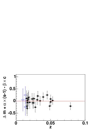
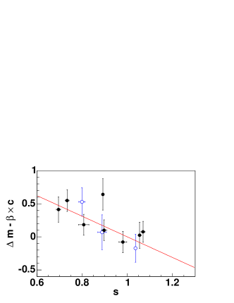
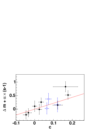
Using $B$- and $V$-band only light curves of supernovae with redshifts larger than 0.015 from the test sample, we obtain: $M_{B}^{70}=-19.41\pm 0.04$, $\alpha=1.56\pm 0.25$ and $\beta=2.19\pm 0.33$. The standard deviation of residuals is $0.16\pm 0.03$ . Uncertainties on $m_{B},s,c$ along with their covariance were included in the fit, we also considered an uncertainty on redshifts due to peculiar velocities of 300 km.s^-1; an additional “intrinsic” dispersion of 0.13 is needed in order to get a $\chi^{2}$ per degree of freedom of 1. The resulting Hubble diagram as well as the observed brighter–slower and brighter–bluer relations are shown figure 4.

Figure 4: From top to bottom: Residuals to the Hubble diagram as a function of redshift, stretch $s$ and color $c$ indexes for supernovae of the test sample fitted in $B$ and $V$ bands. SNe with redshifts smaller than 0.015 are labeled with opened symbols.

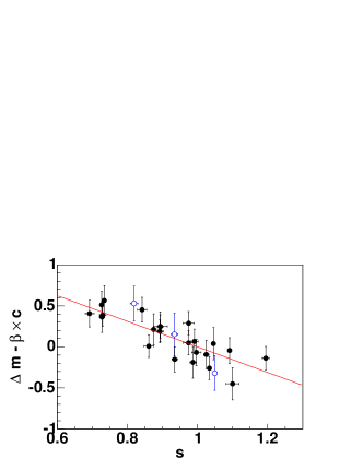
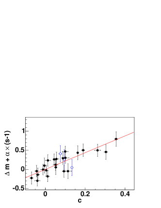
Our approach to estimating distances easily compares to the one adopted in Tripp (1998): the main differences are the light curve model and the brighter-slower parameterization. When we fit the same SNe sample (The Calán-Tololo sample from Hamuy et al. 1996a), a value of $\alpha=1.04\pm 0.24$ and $\beta=2.08\pm 0.27$ are obtained, which compare well to $\alpha=0.88$, $\beta=2.09$ of Tripp (1998), based on peak luminosity, color, and decline rate estimates from Hamuy et al. (1996a). We conclude that our model correctly reproduces basic parameter estimations of previous works.

Concerning the interpretation of the brighter-bluer correlation, we find a value of $\beta$ which is incompatible with $R_{B}=4.1$, expected for extinction by dust analogous to the observed law in the Milky Way. The value we find is compatible with those found in previous works (see Tripp (1998) and references therein). However, as stressed in Riess et al. (1996b), the color excess (or deficit) at maximum should not be interpreted as entirely due to extinction but be corrected for the part of this excess that is correlated with stretch . We measure a stretch-color slope of about 0.2, similar to the relation proposed in Phillips et al. (1999) and can redefine our parameters to account for this correlation:

$$c^{\prime} = c+0.2\,(s-1)$$

$$s^{\prime} = s$$

so that $s^{\prime}$ and $c^{\prime}$ are uncorrelated. The correlation coefficients then become $\alpha^{\prime}=\alpha+0.2\,\beta$ and $\beta^{\prime}=\beta$, which means that redefining the color excess to explicitly assign to stretch the color variations correlated to stretch does not change the brighter-bluer correlation strength.

The two-parameter (stretch and color) pragmatic approach we followed can accommodate both reddening by dust and any intrinsic color effect dependent or not on stretch. One may reasonably assume that reddening by dust and stretch independent intrinsic colors mix (as proposed in Nobili et al. 2003), and that disentangling the contributions would improve the distance resolution. Our distance indicator is however independent of the interpretation of the color variations. Since the low value of $\beta$ may indicate that some intrinsic effect plays a role, we did not interpret color as only due to reddening by dust and hence accepted negative $c$ values as such.

4.1.2 Hubble diagram in $UB$ only

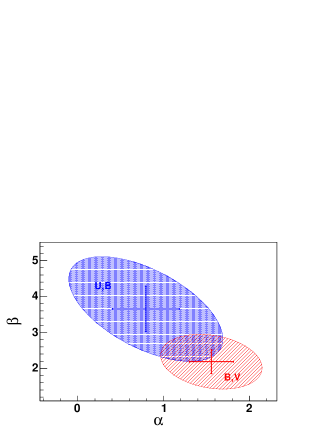
We applied the same procedure as in the previous section to fit the $U$ and $B$-band light curves of the sub-sample of table 2 for which $U$-band measurements are available and redshifts larger than 0.015 (9 supernovae). We obtain $M_{B}^{70}=-19.37\pm 0.05$, $\alpha=0.8\pm 0.4$, $\beta=3.6\pm 0.6$, and the standard deviation of residuals is $0.16\pm 0.05$. As expected, these results are consistent with the fit using $B$ and $V$, as shown by the confidence contours for $\alpha$ and $\beta$ fitted using either $UB$ or $BV$ light curves shown figure 5. Note the covariance between the estimated values of $\alpha$ and $\beta$, particularly in the $U+B$ band case, which simply reflects the correlation between the parameters $c$ and $s$ in the test sample.

One of the SN present in this sample (1996bo) show a large statistical uncertainty due to its limited $U$-band photometry. Removing this point from the fit has the effect of bringing down the $U,B$ contour to the point that it contains almost all of the $B,V$ contour, bringing the two determinations of $\alpha$ and $\beta$ closer to each other.

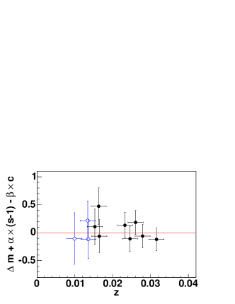
Figure 6 presents the residuals to the Hubble diagram as a function of redshift, stretch and color using the values of $M^{\prime}_{B},\alpha,\beta$ fitted with $B$- and $V$-band light curves in the previous section. Note the large uncertainty affecting 1996bo, which appears as a $\sim 2$ sigma outlier in the 3 plots. Fitting the Hubble diagram with the values of $\alpha$ and $\beta$ obtained with $B$- and $V$-band light curves, the standard deviation of residuals is $0.20\pm 0.05$.

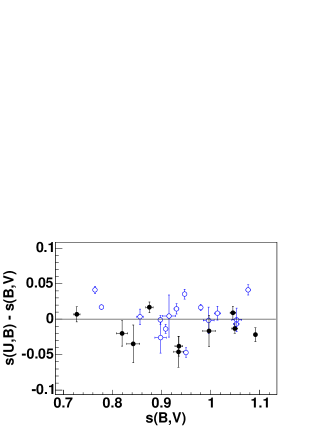
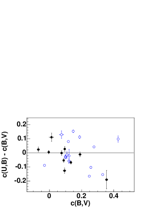
Comparisons of the fitted values of $s$ and $c$ fitted using either $UB$ or $BV$ data are shown figure 7. The error bars only reflect the propagation of photometric errors and do not account for any intrinsic dispersion. There is no significant bias between the two estimates.

Figure 5: 68% joint confidence regions for $(\alpha,\beta)$ fitted using either $UB$ or $BV$ light curves of the test sample. The crosses show the best fitted values with $1\leavevmode\nobreak\ \sigma$ uncertainties.

Figure 6: From top to bottom: Residuals to the Hubble diagram as a function of redshift, stretch $s$ and color $c$ indexes for supernovae of the test sample fitted in $U$ and $B$ bands. The values of $M^{\prime}_{B},\alpha,\beta$ used here are those fitted using $B$ and $V$ bands as described in the text. SNe with redshifts smaller than 0.015 are labeled with opened symbols. Note the large uncertainty affecting one SN (1996bo) due to its limited $U$-band photometry, and which also appears as a $\sim 2$ sigma outlier in the 3 plots.

Figure 7: Differences of $s$ and $c$ values fitted with either $UB$ or $BV$ light curves of supernovae from the training and the test sample (respectively opened and filled symbols). The error bars only reflect the propagation of photometric errors and do not account for any intrinsic dispersion.

4.2 Comparison with other luminosity distance estimators

We compare our method with various estimators of SN Ia distances by examining the dispersions about the Hubble line of a sample of nearby supernovae. The comparison is made on distances measured in $B$ and $V$ bands only for which we obtain a dispersion of $0.16\pm 0.03$. Our $U$- plus $B$-band distances estimates could not be compared with other estimate due to the lack of published distances measured in these 2 bands.

As shown in many papers (e.g. Wang et al. 2003 and Wang et al. 2005), testing luminosity distance indicators on “low-extinction sample” greatly improves their performance. As said in the introduction, cutting on color estimate measured with a redshift dependent accuracy is a source of systematic errors which we need to avoid for cosmological applications. We hence compare our resolutions to “full-sample” resolutions, for distance indicators involving rest-frame $U$, $B$ and $V$ bands.

The MLCS method was originally presented in Riess et al. (1996a), quoting a distance resolution of 0.12. Its latest development is presented in Jha (2002), with a distance resolution of 0.18, and used in Riess et al. (2004). From the latter, we collected the distance measurements to the 20 objects in common with our test sample, and compute a Hubble diagram dispersion of 0.24 (0.22 with the low-redshift “golden sample”) ) to be compared with our value of 0.16 when measured on the same 20 events.

The CMAGIC method of Wang et al. (2003) finds a weighted dispersion of 0.08 for a sub-sample of SNe with $B_{max}-V_{max}<0.05$. With a weaker cut on color, $B_{max}-V_{max}<0.5$, the dispersion rises to about 0.15, which is consistent with our result. Similarly, the $\Delta C_{12}$ method presented in Wang et al. (2005), also present an exquisite distance resolution of 0.07 in the $V$ band based on a low-extinction subsample. However, when considering the full sample, the distance resolution degrades to 0.18. A more detailed comparison with CMAGIC and $\Delta C_{12}$ would require comparing the distances of the same sample of SNe (due to the limited statistics) but their distances are not published. Note also that in these papers, the test and training samples are not separated.

In summary, the method we propose gives a dispersion on distances measured using $B$- and $V$-band data only comparable or lower than obtained with other methods while also providing, for the first time, comparable dispersion values for distances measured using $U$- and $B$-band data only.

5 Conclusion

We have proposed a new method to fit broadband light curves of Type Ia supernovae. It allows us to determine simultaneously the SN Ia rest-frame $B$ magnitude at maximum, stretch and color excess (or deficit) using any measured multi-color light curve within the wavelength range of rest-frame $UBV$ bands. This technique is particularly well-suited to the treatment of high-redshift SNe Ia for which limited coverage is obtained in both wavelength and phase.

The k-corrections, which allow the observer to transform the observed magnitudes into the standard rest-frame magnitudes, are built-in; the model includes the dependence on stretch and color of the spectrum template needed to estimate those corrections. In particular, the well-known correlation between $(U-B)_{max}$ and stretch is reproduced.

The $(B-V)$ and $(V-R)$ stretch-independent colors we obtain are extremely similar to the ones expected from reddening by dust. The $(U-B)$ color departs from this law. We find a relation between $(B-V)$ color and observed $B$ luminosity incompatible with $R_{B}=4.1$, at more than 3 standard deviations, even when accounting for the stretch–color correlation.

We have tested this fitting procedure on an independent sample of SNe Ia. Alternatively using $B$- and $V$-band data and $U$- and $B$-band data, we are able to retrieve consistent parameters and hence build Hubble diagrams with both sets of data. The dispersions about the Hubble line were found to be $0.16\pm 0.03$ and $0.16\pm 0.05$ in the $B$ plus $V$ and $U$ plus $B$ bands only, respectively. This method is particularly well adapted to reliably measure SN Ia distances in the full redshift range and in particular beyond redshift $z\sim 0.8$ for which rest-frame $V$-band measurements are often not available.

Table 1: The training sample of Type Ia supernovae light curves

Name	$z$	Bands	$m^{*}_{B}$	$s$	$c$	Phot. Ref.
1981B	0.006	UBV	12.018 (0.003)	0.911 (0.004)	0.165 (0.002)	(B83)
1984A	-0.001	UBV	12.389 (0.003)	0.946 (0.005)	0.215 (0.003)	(K86)
1986G	0.002	BV	12.026 (0.006)	0.736 (0.005)	0.915 (0.006)	(P87)
1990N	0.003	UBVR	12.701 (0.006)	1.055 (0.005)	0.090 (0.005)	(L91,L98)
1991T	0.006	UBVR	11.574 (0.003)	1.129 (0.005)	0.183 (0.003)	(F92,L98,A04,K04b)
1992A	0.006	UBVR	12.546 (0.003)	0.794 (0.003)	0.088 (0.002)	(S92,A04)
1992al	0.015	BVR	14.448 (0.012)	0.922 (0.011)	-0.035 (0.012)	(H96)
1994D	0.001	UBVR	11.722 (0.002)	0.780 (0.002)	-0.068 (0.002)	(R95,P96,M96,A04)
1994S	0.015	BVR	14.764 (0.017)	1.006 (0.025)	0.011 (0.018)	(R99)
1994ae	0.004	BVR	13.108 (0.008)	0.990 (0.006)	0.098 (0.009)	(R99,A04)
1995D	0.007	BVR	13.450 (0.013)	1.029 (0.014)	0.072 (0.012)	(R99,A04)
1995al	0.005	BVR	13.309 (0.016)	1.038 (0.019)	0.168 (0.017)	(R99)
1996X	0.007	BVR	12.986 (0.010)	0.868 (0.011)	0.050 (0.010)	(R99)
1997E	0.013	UBVR	15.101 (0.006)	0.820 (0.010)	0.078 (0.006)	(J02)
1997do	0.010	UBVR	14.314 (0.014)	0.920 (0.013)	0.118 (0.009)	(J02)
1998bu	0.003	UBVR	12.069 (0.002)	0.989 (0.004)	0.260 (0.002)	(S99)
1998dh	0.009	UBVR	13.825 (0.011)	0.861 (0.006)	0.110 (0.008)	(J02)
1998es	0.011	UBVR	13.814 (0.007)	1.061 (0.009)	0.104 (0.006)	(J02)
1999aa	0.014	UBVR	14.728 (0.005)	1.055 (0.005)	-0.007 (0.005)	(J02,A04,K00)
1999ac	0.009	UBVR	14.114 (0.005)	0.925 (0.009)	0.112 (0.006)	(J02)
1999cc	0.031	UBVR	16.802 (0.009)	0.834 (0.012)	0.047 (0.010)	(J02)
1999cl	0.008	UBVR	14.819 (0.008)	0.901 (0.011)	1.118 (0.007)	(J02,K00)
1999dq	0.014	UBVR	14.398 (0.004)	1.057 (0.006)	0.118 (0.004)	(J02)
1999ee	0.011	UBVR	14.839 (0.003)	0.979 (0.003)	0.297 (0.002)	(S02)
1999ek	0.018	UBVR	15.616 (0.005)	0.888 (0.007)	0.167 (0.005)	(J02,K04b)
2000E	0.005	UBVR	12.856 (0.004)	1.011 (0.006)	0.219 (0.004)	(V03)
2000ca	0.024	UBVR	15.529 (0.007)	1.000 (0.012)	-0.066 (0.006)	(K04a)
2000cn	0.023	UBVR	16.551 (0.008)	0.730 (0.006)	0.195 (0.006)	(J02)
2000dk	0.017	UBVR	15.338 (0.005)	0.727 (0.007)	0.054 (0.005)	(J02)
2001V	0.015	BVR	14.603 (0.019)	1.100 (0.019)	0.113 (0.018)	(Vi03)
2001bt	0.014	BVR	15.267 (0.006)	0.865 (0.005)	0.232 (0.007)	(K04b)
2001cz	0.016	UBVR	15.045 (0.006)	0.995 (0.010)	0.122 (0.007)	(K04b)
2001el	0.004	UBVR	12.600 (0.004)	0.933 (0.004)	0.200 (0.004)	(K03)
2002bo	0.004	UBVR	13.956 (0.005)	0.896 (0.004)	0.443 (0.005)	(Z03,B04,K04b)

Table 2: The test sample of Type Ia supernovae light curves

Name	$z$	$z$	Bands	$m^{*}_{B}\leavevmode\nobreak\ {}^{BV}$	$s\leavevmode\nobreak\ ^{BV}$	$c\leavevmode\nobreak\ ^{BV}$	$m^{*}_{B}\leavevmode\nobreak\ {}^{UB}$	$s\leavevmode\nobreak\ ^{UB}$	$c\leavevmode\nobreak\ ^{UB}$	Phot. Ref.
1990af	0.051	0.050	BV	17.73 (0.01)	0.73 (0.01)	0.00 (0.01)				(H96)
1992bc	0.020	0.020	BVR	15.09 (0.01)	1.03 (0.01)	-0.04 (0.01)				(H96)
1992bh	0.045	0.045	BV	17.60 (0.02)	0.97 (0.02)	0.10 (0.01)				(H96)
1992bo	0.019	0.018	BVR	15.76 (0.01)	0.73 (0.01)	0.06 (0.01)				(H96)
1992bp	0.079	0.079	BV	18.28 (0.01)	0.86 (0.01)	-0.04 (0.01)				(H96)
1993H	0.024	0.025	BVR	16.74 (0.02)	0.69 (0.01)	0.26 (0.02)				(H96,A04)
1993O	0.052	0.053	BV	17.62 (0.01)	0.89 (0.01)	-0.01 (0.01)				(H96)
1993ag	0.049	0.050	BV	17.80 (0.01)	0.89 (0.02)	0.10 (0.02)				(H96)
1995ac	0.050	0.049	BVR	17.04 (0.01)	1.03 (0.01)	0.01 (0.01)				(R99,A04)
1995bd	0.016	0.016	BVR	15.26 (0.01)	0.99 (0.01)	0.30 (0.01)				(R99,A04)
1996bl	0.036	0.035	BVR	16.68 (0.01)	0.97 (0.01)	0.05 (0.01)				(R99)
1996bo	0.017	0.016	UBVR	15.83 (0.01)	0.88 (0.01)	0.36 (0.01)	15.84 (0.01)	0.89 (0.01)	0.16 (0.07)	(R99,A04)
1997E	0.013	0.013	UBVR	15.10 (0.01)	0.82 (0.01)	0.08 (0.01)	15.10 (0.01)	0.80 (0.01)	0.07 (0.02)	(J02)
1998ab	0.027	0.028	UBVR	16.08 (0.01)	0.94 (0.01)	0.09 (0.01)	16.05 (0.02)	0.90 (0.01)	-0.03 (0.02)	(J02)
1999aa	0.014	0.015	UBVR	14.73 (0.01)	1.05 (0.01)	-0.00 (0.01)	14.72 (0.01)	1.05 (0.01)	-0.00 (0.01)	(J02,K00,A00)
1999ac	0.009	0.010	UBVR	14.10 (0.01)	0.93 (0.01)	0.09 (0.01)	14.08 (0.01)	0.89 (0.02)	0.12 (0.02)	(J02)
1999aw	0.038	0.039	BVR	16.75 (0.01)	1.19 (0.01)	0.04 (0.01)				(S02)
1999cc	0.031	0.032	UBVR	16.78 (0.01)	0.84 (0.01)	0.01 (0.01)	16.75 (0.02)	0.81 (0.02)	0.12 (0.03)	(J02)
1999dq	0.014	0.014	UBVR	14.41 (0.01)	1.05 (0.01)	0.13 (0.01)	14.41 (0.01)	1.04 (0.01)	0.06 (0.01)	(J02)
1999ek	0.018	0.018	BVR	15.61 (0.01)	0.89 (0.01)	0.16 (0.01)				(J02,K04b)
1999gp	0.027	0.026	UBVR	16.02 (0.01)	1.09 (0.01)	0.09 (0.01)	16.02 (0.01)	1.07 (0.01)	0.03 (0.01)	(J02,K01)
2000ca	0.024	0.025	UBVR	15.52 (0.01)	1.00 (0.01)	-0.07 (0.01)	15.56 (0.01)	0.98 (0.02)	-0.05 (0.02)	(K04a)
2000cn	0.023	0.023	UBVR	16.55 (0.01)	0.73 (0.01)	0.19 (0.01)	16.56 (0.01)	0.73 (0.01)	0.18 (0.01)	(J02)
2000dk	0.017	0.016	UBVR	15.34 (0.01)	0.73 (0.01)	0.05 (0.01)	15.33 (0.01)	0.70 (0.01)	0.02 (0.01)	(J02)
2001V	0.015	0.016	BVR	14.60 (0.02)	1.10 (0.02)	0.11 (0.02)				(Vi03)
2001ba	0.029	0.031	BV	16.20 (0.01)	0.99 (0.01)	-0.04 (0.01)				(K04a)