Kappa-mechanism excitation of retrograde mixed modes in rotating B-type stars

Abstract

I examine the stability of retrograde mixed modes in rotating B-type stars. These modes can be regarded as a hybrid between the Rossby modes that arise from conservation of vorticity, and the Poincaré modes that are gravity waves modified by the Coriolis force. Using a non-adiabatic pulsation code based around the traditional approximation, I find that the modes are unstable in mid- to late-B type stars, due to the same iron-bump opacity mechanism usually associated with SPB and $\beta$ Cep stars. At one half of the critical rotation rate, the instability for $m=1\ldots 4$ modes spans the spectral types B4 to A0. Inertial-frame periods of the unstable modes range from 100 days down to a fraction of a day, while normalized growth rates can reach in excess of $10^{-5}$.

I discuss the relevance of these findings to SPB and pulsating Be stars, and to the putative Maia class of variable star. I also outline some of the questions raised by this discovery of a wholly-new class of pulsational instability in early-type stars.

1 Introduction

In a recent paper (Townsend, 2005, hereafter T05), I investigated the influence that the rotation-originated Coriolis force exerts over the self-excited oscillations of slowly pulsating B-type (SPB) stars. To maintain a link with historical theoretical studies of SPB stars in which the effects of rotation were overlooked (e.g., Gautschy & Saio, 1993; Dziembowski et al., 1993), the analysis was restricted to those modes that transform continuously into ordinary g modes as the rotation rate is reduced toward zero. Following the classification scheme for low-frequency waves in rotating fluids (e.g., Gill, 1982), these comprise the prograde and retrograde Poincaré modes, the prograde mixed modes, and the Kelvin modes.

The present paper extends the T05 study to one of the types of pulsation mode found only in rotating stars: the retrograde mixed modes, also referred to in the literature as mixed Rossby-Poincaré modes (e.g, Lou, 2000), mixed Rossby-gravity modes (e.g., Gill, 1982), and Yanai modes (e.g., Townsend, 2003a). After providing a brief background to these modes in Section 2, I use an approximation-based method (Sec. 3), very similar to that developed in T05, to investigate their stability in a range of B-type stellar models (Sec. 4). The principal finding (Sec. 5) is that retrograde mixed modes are unstable in mid to late B-type stars, due to the same iron-bump $\kappa$ mechanism responsible for the pulsation of SPB and $\beta$ Cep stars. I discuss and summarize the significance of this result in Section 6.

2 Background

In order to understand the nature of retrograde mixed modes, and why they might be susceptible to $\kappa$-mechanism excitation, it is helpful to review their relationship to the differing classes of low-frequency mode present in rotating stars. These classes comprise the Poincaré, Kelvin, and Rossby modes on the one hand, and the mixed modes (both prograde and retrograde) on the other.

The Poincaré modes rely on a combination of buoyancy and the Coriolis force to restore displaced fluid elements to their equilibrium position. They reduce to ordinary gravity modes in the non-rotating limit, having an angular dependence described by the spherical harmonics $Y^{m}_{\ell}$ with harmonic degree $\ell$ and azimuthal order $m$ satisfying $-\ell+2\leq m\leq\ell$. In light of this correspondence, it is common to refer to the Poincaré modes simply as g modes (e.g., Lee & Saio, 1987; Bildsten et al., 1996).

However, such a designation groups the Poincaré modes with the Kelvin modes, since the latter also reduce to g modes, having $m=-\ell$, in the non-rotating limit. These Kelvin modes, which always propagate in the prograde azimuthal direction, have rather different properties than the Poincaré modes, making it desirable to maintain the distinction between the two. Most significantly, Kelvin modes exhibit geostrophic balance, where the polar component of the Coriolis force remains in balance with the force arising from polar pressure gradients (see, e.g., Gill, 1982). As a result, the horizontal propagation of these modes is dispersion-free, distinguishing them from the dispersive Poincaré modes.

The Rossby modes (or r modes; see Papaloizou & Pringle, 1978) are unlike the Poincaré and Kelvin modes, inasmuch as they do not require buoyancy to restore displaced fluid elements. Instead, they rely on the conservation of the radial component of total vorticity, operating on fluid displacements across the curved level surfaces of the star’s stratification. [See Saio (1982) for a particularly lucid description of this process]. Rossby modes always propagate in the retrograde direction, and in the limit of slow rotation follow the first-order dispersion relation

$$\sigma\approx\frac{2m\Omega}{\ell(\ell+1)}$$ (1)

independent of the internal stellar structure. Here, and throughout the present work, the symbols have the same meaning as in T05; in particular, $\sigma$ is the pulsation angular frequency in the co-rotating frame of reference, and $\Omega$ is the rotation angular frequency. In the same slow-rotation limit, the horizontal velocity fields generated by r modes approximate those produced by the trivial toroidal modes found in non-rotating stars (e.g., Unno et al., 1989), with an angular dependence described by the curl of a radial vector with length $Y^{m}_{\ell}$.

Mixed modes can be regarded as a hybrid between Rossby and Poincaré modes. In the dispersion diagram for low-frequency modes in a rotating star (see Lou, 2000, Fig. 1), they mark the dividing line between the Poincaré modes at higher $\sigma$, and the Kelvin and Rossby modes at lower $\sigma$. At slow rotation rates, the prograde mixed modes behave like Poincaré modes, and are usually classified as the $\ell=-m+1$ g modes. In contrast, the retrograde mixed modes have a Rossby-like character, and are classified as r modes described by the dispersion relation (1) with $\ell=m$. As the rotation rate increases, however, the prograde and retrograde mixed modes for each value of $m$ approach one another in frequency, and exhibit properties that lie somewhere between pure Rossby and Poincaré modes.

There is a well-established body of literature on mixed modes in the field of terrestrial atmospheric and oceanic geophysics, extending back to their detection in the Earth’s atmosphere by Yanai & Maruyama (1966), coupled with the development by Matsuno (1966) of the ‘equatorial $\beta$-plane’ approximation for analytical treatment of low-frequency waves in rotating fluids. Literature discussing mixed modes in a stellar astrophysical context is, however, comparatively scarce. Lee & Saio (1987, 1997) and Dziembowski & Kosovichev (1987) have both noted the presence of r-mode solutions to the governing rotating-star pulsation equations that acquire the character of g modes in the limit of large spin parameter $\nu\equiv 2\Omega/\sigma$. Yet, a full appreciation of the nature of these mixed-mode solutions did not emerge until the $\beta$-plane approximation was applied to the stellar pulsation problem, in the recent studies by Lou (2000) and Townsend (2003a).

From a standpoint of stellar stability, the retrograde mixed modes are particularly interesting on account of their relationship to r modes. Being almost solenoidal (e.g., Saio, 1982), r modes produce little compression or rarefaction of the stellar plasma, and are therefore difficult to excite via the classical ‘Greek letter’ mechanisms ($\gamma$, $\delta$, $\epsilon$ and $\kappa$; see Unno et al., 1989) which involve a thermodynamic Carnot cycle. This explains why incidences of r-mode instability due to these mechanisms are rare. Indeed, even in those situations where classical instability has been found, the strength of the excitation – as measured by its linear growth rate – has been much smaller than is typical for ordinary p or g modes (see, e.g., Berthomieu & Provost, 1983).

However, in the case of retrograde mixed modes the non-solenoidal Poincaré character acquired with more-rapid rotation causes them to generate appreciable compressions and rarefactions. If rotation is sufficient, therefore, these modes stand a good chance of becoming (significantly) unstable to one of the classical excitation mechanisms. This recognition is the foundation for the present paper.

3 Method

The method used to investigate the stability of retrograde mixed modes is based on the so-called ‘traditional approximation’, and is very similar to the approach described in detail in T05. In particular, I solve an identical set of coupled differential equations (7–10, ibid) and boundary conditions (15–16, ibid) as an eigenproblem, using the non-adiabatic boojum code. The resulting dimensionless eigenfrequencies

$$\omega\equiv\sigma\,\sqrt{\frac{R_{\ast}^{3}}{GM_{\ast}}},$$ (2)

define, via their imaginary parts $\omega_{\rm i}$, whether a mixed mode is linearly stable ($\omega_{\rm i}>0$) or unstable ($\omega_{\rm i}<0$). The most important departure from T05 relates to the calculation of the effective harmonic degree $\tilde{\ell}$ appearing in the pulsation equations. In T05, $\tilde{\ell}$ is obtained (eqn. 6, ibid) from the eigenvalue $\lambda^{m}_{\ell}$ of Laplace’s tidal equations that transforms continuously into $\ell(\ell+1)$ in the limit of no rotation.

In the present analysis, I instead evaluate $\tilde{\ell}$ from the family of eigenvalues $\lambda$ that are appropriate to retrograde mixed modes. Within the alternative indexing schemes introduced by Lee & Saio (1997) and Townsend (2003a), they are labeled as the $k=-1$ or $s=0$ solution branches of the tidal equations. Only minor revisions to boojum were required to permit consideration of these branches, consisting primarily of alterations to the matrix routines employed to calculate $\lambda$. However, initial usage of the updated code revealed very poor convergence toward eigenfrequencies, with thousands of relaxation iterations required to reach the desired solution tolerance. After some investigation, the difficulty was traced to the adoption in T05 of the steady-wave approximation. This approximation, which entails using only the real part of the frequency when evaluating $\nu$, permits easy solution of the tidal equations since all variables remain real. However, it has the undesirable side effect that the implicit dependence of $\lambda$ on $\omega$ becomes non-analytic (i.e., $\lambda$ does not satisfy the Cauchy-Riemann equations). Invariably, this tends to hamper the convergence of boojum, especially when considering mixed modes.

This difficulty is addressed within boojum via a new two-stage procedure for evaluation of $\lambda$. First, Laplace’s tidal equations are solved as before using only the real part $\omega_{\rm r}$ of the frequency. The solutions are then taken as the starting point in an inverse iteration algorithm (e.g., Press et al., 1992) based on the fully-complex frequency $\omega$. The algorithm is allowed to run until the relative change in $\lambda$ reaches machine precision, which typically takes five or six iterations. With this modification, $\lambda$ behaves in an analytic fashion, and the convergence issues are wholly resolved.

Further improvements to boojum concern the discriminant root finding process. Although the dimensionless eigenfrequencies of the retrograde mixed modes remain defined by the roots

$$D(\omega)=0$$ (3)

of the discriminant function (see T05, Sec. 2.3), I found that initial isolation of roots was greatly facilitated by adopting the quantity

$$\delta\omega\equiv\frac{\omega_{0}-\omega}{\bar{\Omega}^{3}}$$ (4)

as the independent variable, instead of $\omega$ itself. This quantity, also favoured by Saio (1982), furnishes a normalized measure of departures from the first-order dispersion relation (1). The dimensionless rotation frequency appearing in the denominator is defined as

$$\bar{\Omega}\equiv\Omega\,\sqrt{\frac{R_{\ast}^{3}}{GM_{\ast}}},$$ (5)

while the r-mode limit for mixed modes,

$$\omega_{0}\equiv\frac{2\bar{\Omega}}{m+1},$$ (6)

comes from setting $\ell=m$ in the dispersion relation (1). Since deviations from sphericity arising due to the centrifugal force are neglected in the present analysis, $\omega$ is always smaller than $\omega_{0}$ (see, e.g., Saio, 1982), and thus the ‘departure measure’ $\delta\omega$ is positive for all modes considered.

The algorithm used by boojum to solve the characteristic equation (3) has also been altered. I found that the complex secant approach favoured by Castor (1971) consistently outperforms the Muller (1956) algorithm originally implemented, even though the latter method has a higher (quadratic) order of convergence toward roots.

4 Stellar Models

Figure 1: The theoretical HR diagram for the stellar models introduced in Section 4; these are plotted as points in the effective temperature ($T_{\rm eff}$) versus stellar luminosity ($L_{\ast}$) plane. The dashed lines running diagonally from top left to bottom right indicate the ZAMS and TAMS main sequence limits, while the circle is centred on the position of the 53 Per model analyzed in Section 5.1. Full evolutionary tracks for three selected initial masses (labeled at the ZAMS in solar units) are also shown in the diagram, drawn as solid lines.

I use the Warsaw–New Jersey evolution code to calculate tracks of stellar models for a metalicity $Z=0.02$. These tracks, of which there are 91 together comprising 4268 individual models, sample the initial mass range $M_{\ast}=2.3$–$5.3\,{\rm M}_{\sun}$ at a resolution $0.05\,{\rm M}_{\sun}$ and the range $M_{\ast}=5.3$–$8.3\,{\rm M}_{\sun}$ at a resolution $0.1\,{\rm M}_{\sun}$; each extends from zero-age main sequence (ZAMS) to terminal-age main sequence (TAMS). This coverage of the theoretical Hertzsprung-Russel (HR) diagram, plotted in Fig. 1, is shifted toward rather lower masses than considered in T05, primarily to ensure – based on initial exploratory calculations – that complete coverage of the mixed-mode instability strips is secured (see Sec. 5.2). However, apart from the differences in initial masses, the parameters and input data I adopt for the stellar model calculations are identical to those discussed in Section 3 of T05.

5 Stability Calculations

5.1 53 Per Model

Figure 2: Departure measures for $m=1$ mixed modes of the 53 Per model, plotted as a function of rotation frequency. Each curve corresponds to a particular radial order $n$; the line weight is used to indicate whether modes are stable (thin) or unstable (thick).

I first apply the updated boojum code to investigate the stability of $m=1$ mixed modes in the same 53 Per-like model introduced in T05. A range of rotation angular frequencies, from the negligibly rotating case up to the half-critical rate $\Omega/\Omega_{\rm c}=0.5$, is considered. This upper bound is loosely dictated by the limitations of the approximations described in Section 3 (and see also T05), but also happens to be close to the observed ceiling on SPB-star rotation, $\Omega/\Omega_{\rm c}\approx 0.46$, established by the B5 pulsator HD 1976 (Mathias et al., 2001).

The results from these stability calculations are plotted in Fig. 2, which traces the $\Omega$ dependence of the eigenfrequency departure measure $\delta\omega$ introduced in eqn. (4), for modes of differing radial orders $n$. At slowest rotation, the flatness of the $\delta\omega$ curves indicates that the departure measure for each mode is independent of $\Omega$, confirming the finding by Papaloizou & Pringle (1978) that deviations from the first-order dispersion relation (1) vary as $\mathcal{O}(\Omega^{3})$. Toward more-rapid rotation, higher-order terms become significant, with the result that the curves shown in Fig. 2 dip downward.

Of particular interest in the figure is the fact that a group of modes, having radial orders $n=13$–25, become unstable above a rotation rate $\Omega/\Omega_{\rm c}\approx 0.3$. The nature of the instability is revealed in Fig. 3, which plots both the cumulative work $W$ and differential work ${\rm d}W/{\rm d}x$ for the $n=20$ mixed mode, at a rotation rate $\Omega/\Omega_{\rm c}=0.25$ when the mode is stable, and at the more-rapid rate $\Omega/\Omega_{\rm c}=0.5$ when the mode has subsequently been destabilized. The sharp peak in ${\rm d}W/{\rm d}x$ at $\log T\approx 5.3$ reveals that the mode is strongly driven by the same iron-bump opacity mechanism considered responsible for the p-mode instability of $\beta$ Cep stars (Cox et al., 1992; Dziembowski & Pamiatnykh, 1993) and the g-mode instability of SPB stars (Gautschy & Saio, 1993; Dziembowski et al., 1993).

As elucidated by the latter-most authors (and see also Pamyatnykh, 1999), two key requirements must be satisfied for the $\kappa$ mechanism to be effective. First, the relative Lagrangian pressure perturbation $\delta p/p$ should be large and vary slowly with radius within the driving zone. This constraint on the shape of the eigenfunction establishes a lower limit $n\geq 13$ on the radial order of unstable mixed modes in the 53 Per model, surprising similar to the corresponding limit found in T05 for unstable g modes. In fact, the coincidence between the two stems from the fact that the same set of pulsation equations governs both classes of mode.

The second requirement is that the pulsation period should not be significantly greater than the local thermal timescale within the excitation zone. If instead the period is too long, radiative diffusion between neighbouring fluid elements can lead to strong damping in the inner envelope, that cancels out any driving due to the $\kappa$ mechanism. This inhibition effect is illustrated in Fig. 3. The strength of the $\kappa$-mechanism driving is the same in both panels, as can be seen from the similar peaks ${\rm d}W/{\rm d}x\approx 0.04\,E_{W}$ in the differential work at $\log T\approx 5.3$. However, the radiative damping at $\log T\approx 5.7$ is more pronounced in the left-hand panel, owing to the longer period of the mode – $P=2.76\,\rm d$, as compared to $P=1.63\,\rm d$ for the right-hand panel. This enhanced damping is sufficient to stabilize the mode.

All mixed modes in Fig. 2 having $\Omega/\Omega_{\rm c}\lesssim 0.3$ or $\delta\omega\gtrsim 4$ posses periods longer than the thermal timescale in the driving zone. Hence, these modes are stabilized by the same radiative damping described above. In the following section, I explore how radiative damping, acting in tandem with the restriction on the $\delta p/p$ eigenfunction morphology, shapes which regions of the HR diagram exhibit mixed-mode instability via the $\kappa$-mechanism. The remainder of the present section is focused on a discussion of the unstable $n=1$ mixed mode seen in Fig. 2 as the thick line having $\delta\omega\approx 0$.

Figure 3: The cumulative work (thin) and differential work (thick) for the $m=1$, $n=20$ mixed mode of the 53 Per model, plotted as a function of temperature at rotation rates $\Omega/\Omega_{\rm c}=0.25$ (left panel) and 0.5 (right panel). The work functions are expressed in scaled units of the total energy of pulsation $E_{W}$.

Inspection of the work function for this mode indicates that weak driving in the core, at $\log T\approx 7.4$, is responsible for the instability. Although this may be a result of genuine $\epsilon$-mechanism excitation, the normalized growth rate of the mode,

$$\eta\equiv-\omega_{\rm i}/\omega_{\rm r},$$ (7)

never exceeds $3.3\times 10^{-13}$ at any rotation rate considered (compare with the $n=20$ mode, which reaches $\eta=7.3\times 10^{-6}$ at $\Omega/\Omega_{\rm c}=0.5$). This value differs so little from zero that it would be more accurate to describe the $n=1$ mixed mode as neutrally stable. Such a stance is lent support by the fact that the mode sits very close to the pure r-mode limit $\omega=\omega_{0}$, and – being almost solenoidal – can be expected to be neither excited nor damped by classical mechanisms.

5.2 Instability Strips

Figure 4: Instability strips in the HR diagram, for $m=1\ldots 4$ mixed modes of the stellar models introduced in Section 4. For each value of the azimuthal order, the extent of the $\kappa$-mechanism instability at the rotation rates $\Omega/\Omega_{\rm c}=0.25$ (dotted) and 0.5 (dashed) is indicated using thick lines. The small open triangles, filled squares, and open diamond show the inferred positions of selected SPB stars, pulsating Be stars, and HD 208727, respectively (see text).

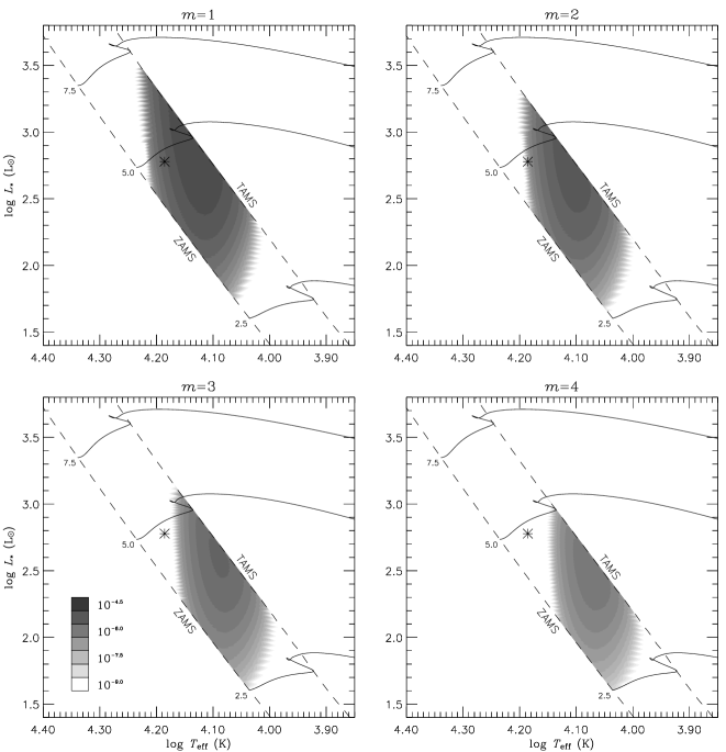
Figure 5: Maximal growth rates in the HR diagram, for $m=1\ldots 4$ mixed modes of the stellar models introduced in Section 4. For each value of the azimuthal order, the largest $\eta$ at the rotation rate $\Omega/\Omega_{\rm c}=0.5$ is indicated via the gray level. The distribution of these levels is logarithmic, and extends from $10^{-9}$ (white) to $10^{-4.5}$ (black).

Figure 6: Instability regions in the $T_{\rm eff}-P_{\rm i}$ plane, for $m=1\ldots 4$ mixed modes of the stellar models introduced in Section 4. For each value of the azimuthal order, the extent of the $\kappa$-mechanism instability at the rotation rates $\Omega/\Omega_{\rm c}=0.25$ (dotted) and 0.5 (dashed) is indicated using thick lines. The small open triangles, filled squares, and open diamond show the observed periods of selected SPB stars, pulsating Be stars, and HD 208727, respectively (see text). Note that the ordinate scale is logarithmic.

The scope of the investigation is now broadened, to encompass the entire set of stellar models introduced in Section 4. I use boojum to investigate the stability of these models toward $m=1\ldots 4$ retrograde mixed modes. Fig. 4 plots the instability strips in the HR diagram associated with these modes, at two distinct rotation rates: $\Omega/\Omega_{\rm c}=0.5$ approximates the observed upper limit on SPB-star rotation (see Sec. 5.2), while $\Omega/\Omega_{\rm c}=0.25$ is representative of more-moderately rotating stars. Formally, the condition of instability is defined by the requirement that a mode has a positive growth rate. However, it is appropriate to exclude those modes that, similar to the $n=1$ mode considered in the preceding section, have such small values of $\eta$ that they are more properly regarded as neutrally stable. Therefore, the instability strips shown in Fig. 4 are constructed to enclose all stellar models that possess one or more modes with a growth rate in excess of the threshold value $\eta=10^{-9}$.

Also shown in Fig. 4 are the inferred positions of selected SPB and pulsating Be stars, and the position of the Maia candidate star HD 208727, which is discussed further in Section 6. The SPB data are compiled directly from the tabulations by Waelkens et al. (1998), Aerts et al. (1999), Mathias et al. (2001) and De Cat & Aerts (2002); in the many cases where multiple $(T_{\rm eff},L_{\ast})$ values exist for a given star, the most recently published ones are adopted. The pulsating Be-star data are obtained via a three-stage process. First, the list of line-profile variable Be stars observed by Rivinius et al. (2003) is merged with that of the short-period photometric variables studied by Percy et al. (2002); Percy et al. (2004). Then, the calibrations by Chauville et al. (2001) are used to determine the effective temperature and surface gravity of each star in the merged list; if values are not available for a given star, it is dropped from the list. Finally, I define an empirical relation $L_{\ast}=L_{\ast}(T_{\rm eff},\log g)$ via a quintic surface fit to the luminosity data of the stellar models introduced in Section 4. This relation is used to map the $(T_{\rm eff},\log g)$ values in the list into corresponding $(T_{\rm eff},L_{\ast})$ values, suitable for plotting in the HR diagram.

Figure 4 demonstrates that the mixed-mode instability found in the 53 Per model (Sec. 5.1) extends to many of the other stellar models considered. At a rotation rate $\Omega/\Omega_{\rm c}=0.25$, the instability for the $m=1\ldots 4$ modes spans the effective temperature range $\log T_{\rm eff}=3.96$–$4.17$. At the more-rapid rate $\Omega/\Omega_{\rm c}=0.5$, the instability broadens and shifts to toward higher effective temperatures and luminosities, with a range $\log T_{\rm eff}=3.99$–$4.23$ corresponding loosely to spectral types B4 to A0 (Böhm-Vitense, 1981). At fixed rotation rate, incrementing the azimuthal order displaces the instability in the opposite direction, toward lower effective temperatures and luminosities.

The sensitivity of the instability toward both rotation rate and azimuthal order comes from the period matching requirement discussed in the preceding section. Returning once again to the first-order dispersion relation (1), it is clear that any increase in $\Omega$ ($m$) will act to increase (decrease) the frequency of a mixed mode, and hence to shorten (lengthen) its period. To ensure that this period remains commensurate with the local thermal timescale in the driving zone, the instability therefore shifts to hotter (cooler) stars, in which the opacity bump is situated shallower (deeper) in the envelope. A very similar line reasoning was employed in T05 to understand the behaviour of the instability strips for Poincaré, Kelvin and prograde mixed modes.

Table 1: Proportions, expressed as percentages, of the SPB (Be) stars that fall within the mixed-mode instability strips plotted in Fig. 4, for each azimuthal order and rotation rate considered.

	$m$
$\Omega/\Omega_{\rm c}$	1	2	3	4
0.25	41 (3)	13 (0)	3 (0)	1 (0)
0.50	67 (7)	48 (3)	41 (3)	29 (3)

Examining the correspondence between the mixed-mode instability strips and the positions of the selected pulsating stars plotted in Fig. 4, it is clear that there is not a great deal of agreement between the two. This discrepancy is underlined by Table 1, which summarizes the proportion of stars enclosed by the instability strips at each azimuthal order and rotation rate considered. At best, the strips encompass only two thirds of the SPB stars – a reflection of the stars’ bias toward the late end of the B spectral type, whereas SPB stars tend to be concentrated more around the mid-B types. In fact, the SPB stars coincide far more closely with the theoretical instability strips predicted for $\kappa$-mechanism excitation of ordinary g modes (see Pamyatnykh, 1999, his figs. 3 & 4). Therefore, it seems unlikely that the SPB phenomenon as a whole can be explained better by mixed modes than by the widely-accepted g-mode interpretation.

The situation is superficially similar for the pulsating Be stars shown in Fig. 4; in no case do more than 7 percent of these stars fall within the mixed-mode instability strips. In light of the concentration of Be stars toward the early-B spectral types (Porter, 1996), and the conspicuous absence of any pulsating Be stars later than spectral type B6 (see Baade, 1989a, b; Porter & Rivinius, 2003, and references therein), this result is hardly surprising. However, in contrast to SPB stars, Be stars are known to rotate at a significant fraction of their critical rate ($\langle V_{\rm e}/V_{\rm c}\rangle\approx 0.83$, corresponding to $\langle\Omega/\Omega_{\rm c}\rangle\approx 0.96$; see Chauville et al., 2001). Although near-critical rotation lies beyond the reach of the boojum code, the general trends shown in Fig. 4 suggest that as $\Omega/\Omega\rightarrow 1$ the mixed-mode instability strips should shift toward the early-B spectral types, encompassing a much greater proportion of pulsating Be stars. Therefore, it remains plausible that the variability of these stars can be attributed to mixed modes, rather than the Poincaré modes that are usually supposed (e.g., Rivinius et al., 2003, and references therein). This possibility is returned to in Section 6.

Having discussed the extent of the $\kappa$-mechanism instability, I now shift the focus to its strength. Fig. 5 plots the maximal growth rates of the instability across the HR diagram, for the $m=1\ldots 4$ mixed modes at the rotation rate $\Omega/\Omega_{\rm c}=0.5$. These values are intended to furnish some measure of the robustness of the instability. To this end, Dziembowski et al. (1993) employ the normalized growth rate introduced by Stellingwerf (1979), but in the absence of any sound theory of non-linear amplitude saturation, I prefer to adhere to the simple definition (7).

The general trend seen in the figure is that the growth rates are at their greatest for the $m=1$ modes, reaching up to a value $\eta\approx 10^{-4.5}$ that is commensurate with the strongest instabilities associated with $\beta$ Cep and SPB stars. Toward larger values of $m$, $\eta$ declines rapidly, reflecting the fact that mixed modes having larger azimuthal orders exhibit a more Rossby-like character (see, e.g. Lou, 2000, Fig. 1; note that the horizontal wavenumber $k_{x}$ plotted as abscissa is equivalent to $m$), and are therefore (Sec. 2) more difficult to excite via the $\kappa$ mechanism.

A secondary trend in Fig. 5 is that the growth rates appear systematically larger for the stellar models situated near the TAMS. As shown in Fig. 4 of T05, these models are characterized by driving-zone thermal timescales that are rather longer than the corresponding ZAMS models. Presumably, mixed modes can satisfy the period matching requirement more easily at these long timescales, and therefore are less susceptible to inhibition arising from radiative damping in the inner envelope.

To bring the present section to a close, Fig. 6 plots the mixed-mode instability regions in the $T_{\rm eff}-P_{\rm i}$ plane. Here,

$$P_{\rm i}\equiv-2\pi/(\sigma-m\Omega)$$ (8)

is the pulsation period in an inertial frame of reference – a quantity of relevance to the observational community, since it can be ascertained directly from time-series monitoring of variable stars. The minus sign appears in this expression because, for the mixed modes considered here, the co-rotating frame frequency $\sigma$ is always smaller than $m\Omega$. Also shown in the figure are the observed periods of the same stars plotted in Fig. 4; in cases where a star is multiperiodic, only the principal period is displayed.

The figure reveals that the inertial frame periods become shorter with rotation rate, behaviour arising due to the appearance of $\Omega$ in the denominator of the expression (8) for $P_{\rm i}$. More significantly, it is evident that the unstable $m=1$ mixed modes exhibit periods that are one or two orders of magnitude larger than those with azimuthal orders $m\geq 2$. This is a consequence of the fact that the $m=1$ modes have co-rotating frame frequencies that, to first order in $\Omega$, follow $\sigma\approx\Omega$ (see eqn. 1). Hence, the denominator in equation (8) involves cancellation between two nearly equal terms, leading to very large inertial-frame periods.

As Fig. 6 demonstrates, these long periods are incompatible with the much-shorter periods ($\sim 1\,\rm d$) observed in SPB stars. While the mismatch between theory and observations might be corrected by considering rotation rates above the present upper limit $\Omega/\Omega_{\rm c}=0.5$, such rapid rotation would be difficult to reconcile with the angular frequencies $\Omega/\Omega_{\rm c}\lesssim 0.25$ more typical to the majority of SPB stars (e.g., Aerts et al., 1999; De Cat et al., 2005). The situation is not much improved for azimuthal orders $m\geq 2$, due to the fact that the instability regions at $\Omega/\Omega_{\rm c}=0.25$ – a more representative rotation rate – are situated at temperatures too cool to encompass many SPB stars. These findings amount to further evidence against a mixed-mode interpretation for the SPB phenomenon.

The periods of the unstable $m=1$ mixed modes in Fig. 6 are also much longer than those observed in pulsating Be stars. At the more-rapid rotation rates representative of these stars, it seems likely that this period discrepancy will be resolved. However, the $m\geq 2$ mixed modes, which match the typical observed periods quite well when $\Omega/\Omega_{\rm c}=0.5$ (even though the $T_{\rm eff}$ range of the instability is too cool), may then become inconsistent with the observations. This is one issue that will have to be addressed if mixed modes are considered a viable explanation for Be-star pulsation.

6 Discussion and Summary

In the preceding sections, I use the non-adiabatic boojum code to explore the stability of $m=1\ldots 4$ mixed modes in rotating B-type stars. The principal finding is that these modes are excited by the same iron-bump $\kappa$ mechanism responsible for the pulsation of SPB and $\beta$ Cep stars. This finding is significant, representing the discovery of a wholly-new type of instability in the early-type domain of the HR diagram.

However, I should emphasize certain caveats relating to this discovery. As discussed in detail in T05, many approximations are employed to derive the system of pulsation equations and boundary conditions solved by boojum. Although these approximations are required for the problem to be tractable using present-day computational resources, they do mean that the results presented here should be regarded as more qualitative than quantitative.

In particular, neglect of the centrifugal deformation of the equilibrium stellar structure will certainly introduce a degree of error in the calculated eigenfrequencies. This is because r modes – and by extension mixed modes – tend to be rather sensitive to any departures from a spherically-symmetric equilibrium state (Provost et al., 1981). Furthermore, the results may be influenced by the incidence of differential rotation (recently discovered in seismic analyses of two $\beta$ Cep stars; see Dupret et al., 2004; Pamyatnykh et al., 2004), although it is as yet unclear what specific effect any departure from the assumed-uniform rotation might have.

Nevertheless, while there certainly remains a great deal of scope for improving upon the theoretical foundation established in the present work, the case for the physicality of the mixed-mode instability in B-type stars is, I believe, convincing. Therefore, it is appropriate to discuss what implications it might have for studies of dynamical phenomena in early-type stars.

As already made clear in the preceding section, I am skeptical that mixed modes can furnish a better explanation for the SPB phenomenon than the currently-accepted model of $\kappa$ mechanism excitation of (predominantly) $\ell=1$ g modes. The latter model has already proven very successful both in matching the observed distribution of SPB stars in the HR diagram (see Pamyatnykh, 1999), and in reproducing the variability exhibited by these stars (see Townsend, 2002; De Cat et al., 2005). Of course, this is not to say that there might not be some SPB stars that turn out to be mixed mode rather than g mode pulsators. In particular, the so-called rapidly rotating Hipparcos SPBs (see Aerts et al., 1999) may, upon closer scrutiny, be found to fall into this category. A thorough evaluation of such a possibility must await new tools for analyzing the spectroscopic and photometric variations generated by mixed modes. These tools should prove relatively straightforward to derive from already-existing models based around the traditional approximation (see Townsend, 1997, 2003b).

The prospects for a mixed-mode role in pulsating Be stars seem rather more favourable. Near-critical rotation should shift the instability strips toward hotter temperatures and earlier spectral types, thereby allowing them to encompass a greater proportion of these stars. There may be difficulty in matching periods, and it has yet to be ascertained whether mixed modes can reproduce observed Be-star line profile variations to the same degree that Poincaré modes already have (see, e.g., Rivinius et al., 2001; Maintz et al., 2003). However, in anticipation of the eventual resolution of these uncertainties, it is worthwhile reflecting on the part played by mixed modes in the episodic, disk-forming mass loss from Be stars (see Porter & Rivinius, 2003, and references therein). Following on from suggestions made by Osaki (1986), Owocki (2004, 2005) has recently advanced a hydrodynamical model for ‘pulsationally driven orbital mass ejection’ (PDOME), in which the addition of a pulsation-originated perturbation to the equatorial regions of a near-critical rotating star is sufficient to lift surface material into orbit. This material gradually diffuses outward under the influence of viscosity (see Lee et al., 1991; Porter, 1999, and references therein), to form a disk with the same Keplerian velocity distribution inferred from observations of Be stars (e.g., Dachs et al., 1986; Hanuschik, 1996).

As demonstrated by Owocki (2005), a key ingredient in the success of the PDOME mechanism is that the azimuthal velocity perturbation is in the prograde direction when the density perturbation is maximal. It would therefore seem that prograde pulsation modes are required for mass ejection to occur, which is problematical to reconcile with observations (Rivinius et al., 2003, and references therein) that indicate retrograde-propagating modes in Be stars. However, an important distinction should be made here between group and phase velocities. While these velocities share the same sign in the case of Poincaré, Kelvin and prograde mixed modes, the retrograde mixed modes behave differently: their phase velocity is (by definition) in the retrograde direction, yet their group velocity is oriented in the opposite direction (see, e.g., Gill, 1982), with maximal density coinciding with prograde azimuthal velocity. Hence, they are able simultaneously to fulfill both the observational constraint of retrograde phase velocity, and the theoretical PDOME constraint of prograde group velocity. In tandem with a re-evaluation of the degree to which Be stars approach critical rotation (see Townsend et al., 2004), retrograde mixed modes may therefore be the missing link required for Owocki’s PDOME mechanism to operate.

Looking now at the opposite, low-temperature end of the B spectral type, mixed modes may also have a role to play in the phenomenon of Maia stars. Struve (1955) first put forward the suggestion that there exists an instability strip in the HR diagram, characterized by pulsation periods on the order of hours, that extends from late-B types to the early-A types. Although the strip was named for its archetype Maia (20 Tau), subsequent observations (e.g., Struve et al., 1957) of this particular star have, rather ironically, revealed it most likely to be non-variable. Other searches for stellar variability in the hypothetical Maia strip (e.g., McNamara, 1985; Lehmann et al., 1995; Percy & Wilson, 2000) have been largely unsuccessful. However, there are a handful of variable stars (e.g., $\gamma$ CrB – Scholz et al., 1998; HD 208727 – Kallinger, Reegen & Weiss, 2002) that remain situated in the strip, and it would therefore be premature to dismiss the Maia-star concept as mere will-o’-the-wisp.

The discovery of the retrograde mixed-mode instability may provide a theoretical framework for understanding the origins of the elusive Maia stars. On the basis of the stellar parameters quoted by Kallinger et al. (2002), the Maia candidate HD 208727 falls blueward of the ZAMS boundary in the HR diagram (see Fig. 4). However, if this boundary were shifted to hotter temperatures, for instance by considering a helium-enriched main sequence, the star would fall well inside the $m=1\ldots 4$ mixed-mode instability regions. Furthermore, the star’s $7.6\,\rm h$ photometric period would be consistent with the inertial frame periods (Fig. 6) typical to $m=3$ and $m=4$ mixed modes for $\Omega/\Omega_{\rm c}=0.5$ (in fact, the star probably rotates rather faster than this, $\Omega/\Omega_{\rm c}\gtrsim 0.67$). Accordingly, although Kallinger et al. (2002) were dismissive of the ability of ordinary g modes to explain the variability of HD 208727, it appears that a mixed-mode interpretation may furnish a good match.

The interpretation of Maia stars as mixed-mode pulsators is lent indirect support in a recent paper by Aerts & Kolenberg (2005), who point out that significant rotation – a prerequisite for the mixed-mode instability – appears to be a common factor in these stars. These authors then proceed to suggest that the Maia stars may simply be an extension of the SPB phenomenon to lower $T_{\rm eff}$ arising due to the Coriolis force. The results presented in T05 would appear to rule out this latter possibility, by demonstrating (Fig.3, ibid) that any Coriolis-originated extension to the SPB instability strip is insufficient to encompass the Maia stars. However, as Figs. 4 and 6 of the present paper illustrate, the mixed-mode instability at larger azimuthal orders ($m\gtrsim 4$) can encompass cooler temperatures corresponding to early A spectral types, while at the same time exhibiting pulsation periods of a few hours. Although this establishes a case for a link between mixed modes and Maia stars, there should – as Aerts & Kolenberg (2005) themselves point out – be a significant improvement in observational datasets before firm conclusions can be reached concerning this issue.

Of course, irrespective of whether retrograde mixed modes have any connection with the Maia phenomenon, there are many pertinent questions that are raised by the discovery of their $\kappa$-mechanism instability. What kinds of variability – spectroscopic or photometric – do these modes generate? Although the majority of SPB stars appear to be well understood as g mode pulsators, are there some that can be better better explained in terms of mixed mode excitation? Might mixed modes explain the variability and mass loss of pulsating Be stars? Can we expect mixed modes in other types of object, such as $\gamma$ Dor stars? I touch on some of these questions in the foregoing analysis, and hope further to address them, and others, in forthcoming papers.

Note added during revision

A recent preprint by Savonije (2005) also investigates mixed-mode instability in early-type stars. Although there are some differences in the specific methodology and results, the general findings are in agreement with those reported in the present work.

References

- Aerts et al. (1999) Aerts C., De Cat P., Peeters E., Decin L., De Ridder J., Kolenberg K., Meeus G., Van Winckel H., Cuypers J., Waelkens C., 1999, A&A, 343, 872
- Aerts & Kolenberg (2005) Aerts C., Kolenberg K., 2005, A&A, 431, 615
- Andersson (1998) Andersson N., 1998, ApJ, 502, 708
- Baade (1989a) Baade D., 1989a, A&AS, 79, 423
- Baade (1989b) Baade D., 1989b, A&A, 222, 200
- Berthomieu & Provost (1983) Berthomieu G., Provost J., 1983, A&A, 122, 199
- Bildsten et al. (1996) Bildsten L., Ushomirsky G., Cutler C., 1996, ApJ, 460, 827
- Böhm-Vitense (1981) Böhm-Vitense E., 1981, Ann. Rev. Astron. Astrophys., 19, 295
- Castor (1971) Castor J. I., 1971, ApJ, 166, 109
- Chauville et al. (2001) Chauville J., Zorec J., Ballereau D., Morrell N., Cidale L., Garcia A., 2001, A&A, 378, 861
- Cox et al. (1992) Cox A. N., Morgan S. M., Rogers F. J., Iglesias C. A., 1992, ApJ, 393, 272
- Dachs et al. (1986) Dachs J., Hanuschik R., Kaiser D., Rohe D., 1986, A&A, 159, 276
- De Cat & Aerts (2002) De Cat P., Aerts C., 2002, A&A, 393, 965
- De Cat et al. (2005) De Cat P., Briquet M., Daszyńska-Daszkiewicz J., Dupret M. A., de Ridder J., Scuflaire R., Aerts C., 2005, A&A, 432, 1013
- Dupret et al. (2004) Dupret M.-A., Thoul A., Scuflaire R., Daszyńska-Daszkiewicz J., Aerts C., Bourge P.-O., Waelkens C., Noels A., 2004, A&A, 415, 251
- Dziembowski & Kosovichev (1987) Dziembowski W., Kosovichev A., 1987, Act. Astron., 37, 313
- Dziembowski et al. (1993) Dziembowski W. A., Moskalik P., Pamyatnykh A. A., 1993, MNRAS, 265, 588
- Dziembowski & Pamiatnykh (1993) Dziembowski W. A., Pamiatnykh A. A., 1993, MNRAS, 262, 204
- Gautschy & Saio (1993) Gautschy A., Saio H., 1993, MNRAS, 262, 213
- Gill (1982) Gill A. E., 1982, Atmosphere-Ocean Dynamics. Academic Press, London
- Hanuschik (1996) Hanuschik R. W., 1996, A&A, 308, 170
- Kallinger et al. (2002) Kallinger T., Reegen P., Weiss W. W., 2002, A&A, 388, L37
- Lee et al. (1991) Lee U., Osaki Y., Saio H., 1991, MNRAS, 250, 432
- Lee & Saio (1987) Lee U., Saio H., 1987, MNRAS, 224, 513
- Lee & Saio (1997) Lee U., Saio H., 1997, ApJ, 491, 839
- Lehmann et al. (1995) Lehmann H., Scholz G., Hildebrandt G., Klose S., Panov K. P., Reimann H.-G., Woche M., Ziener R., 1995, A&A, 300, 783
- Lou (2000) Lou Y., 2000, ApJ, 540, 1102
- Maintz et al. (2003) Maintz M., Rivinius T., Štefl S., Baade D., Wolf B., Townsend R. H. D., 2003, A&A, 411, 181
- Mathias et al. (2001) Mathias P., Aerts C., Briquet M., De Cat P., Cuypers J., Van Winckel H., Flanders. Le Contel J. M., 2001, A&A, 379, 905
- Matsuno (1966) Matsuno T., 1966, J. Meteorol. Soc. Japan, 44, 25
- McNamara (1985) McNamara B. J., 1985, ApJ, 289, 213
- Muller (1956) Muller D. E., 1956, Math. Tab. & Aids to Comp., 10, 208
- Osaki (1986) Osaki Y., 1986, PASP, 98, 30
- Owocki (2004) Owocki S. P., 2004, in Maeder A., Eenens P., eds, Proc. IAU Symp. 215, Stellar Rotation. Astron. Soc. Pac., San Francisco, p. 515
- Owocki (2005) Owocki S. P., 2005, in Ignace R., Gayley K. G., eds, ASP Conf. Ser. 337, The Nature and Evolution of Disks around Hot Stars. Astron. Soc. Pac., San Francisco, in press
- Pamyatnykh (1999) Pamyatnykh A. A., 1999, Act. Astron., 49, 119
- Pamyatnykh et al. (2004) Pamyatnykh A. A., Handler G., Dziembowski W. A., 2004, MNRAS, 350, 1022
- Papaloizou & Pringle (1978) Papaloizou J., Pringle J. E., 1978, MNRAS, 182, 423
- Percy et al. (2004) Percy J. R., Harlow C. D. W., Wu A. P. S., 2004, PASP, 116, 178
- Percy et al. (2002) Percy J. R., Hosick J., Kincaide H., Pang C., 2002, PASP, 114, 551
- Percy & Wilson (2000) Percy J. R., Wilson J. B., 2000, PASP, 112, 846
- Porter (1996) Porter J. M., 1996, MNRAS, 280, L31
- Porter (1999) Porter J. M., 1999, A&A, 348, 512
- Porter & Rivinius (2003) Porter J. M., Rivinius T., 2003, PASP, 115, 1153
- Press et al. (1992) Press W. H., Teukolsky S. A., Vetterling W. T., Flannery B. P., 1992, Numerical Recipes in Fortran, 2 edn. Cambridge University Press, Cambridge
- Provost et al. (1981) Provost J., Berthomieu G., Rocca A., 1981, A&A, 94, 126
- Rivinius et al. (2003) Rivinius T., Baade D., Štefl S., 2003, A&A, 411, 229
- Rivinius et al. (2001) Rivinius T., Baade D., Štefl S., Townsend R. H. D., Stahl O., Wolf B., Kaufer A., 2001, A&A, 369, 1058
- Saio (1982) Saio H., 1982, ApJ, 256, 717
- Savonije (2005) Savonije G. J., 2005, A&A, in press, astro-ph/0506153
- Scholz et al. (1998) Scholz G., Lehmann H., Hildebrandt G., Panov K., Iliev L., 1998, A&A, 337, 447
- Stellingwerf (1979) Stellingwerf R. F., 1979, ApJ, 227, 935
- Struve (1955) Struve O., 1955, Sky Telesc., 14, 461
- Struve et al. (1957) Struve O., Sahade J., Lynds C. R., Huang S. S., 1957, ApJ, 125, 115
- Townsend (1997) Townsend R. H. D., 1997, MNRAS, 284, 839
- Townsend (2002) Townsend R. H. D., 2002, MNRAS, 330, 855
- Townsend (2003a) Townsend R. H. D., 2003a, MNRAS, 340, 1020
- Townsend (2003b) Townsend R. H. D., 2003b, MNRAS, 343, 125
- Townsend (2005) Townsend R. H. D., 2005, MNRAS, 360, 465 (T05)
- Townsend et al. (2004) Townsend R. H. D., Owocki S. P., Howarth I. D., 2004, MNRAS, 350, 189
- Unno et al. (1989) Unno W., Osaki Y., Ando H., Saio H., Shibahashi H., 1989, Nonradial Oscillations of Stars, 2 edn. University of Tokyo Press, Tokyo
- Waelkens et al. (1998) Waelkens C., Aerts C., Kestens E., Grenon M., Eyer L., 1998, A&A, 330, 215
- Yanai & Maruyama (1966) Yanai M., Maruyama T., 1966, J. Meteorol. Soc. Japan, 44, 291