Preface

This thesis is submitted in partial fulfillment of the PhD degree at the Niels Bohr Insitute in Denmark. The thesis concludes three years of work, of which two years were dedicated to scientific work and one year to lecturing and various other duties. The PhD project was carried out under supervision of Professor Åke Nordlund, in the Computational Astrophysics group at the Niels Bohr institute in Copenhagen, Denmark. As part of the PhD education, I spent 4 months at the National Space Science and Technology Center (NSSTC) in Huntsville Alabama, USA. Here I collaborated with the gamma-ray group under Dr. Gerald J. Fishman and in particular with Dr. Ken-Ichi Nishikawa.

The backbone of the thesis consists of three papers published in ApJL (the Astrophysical Journal Letters), plus recent work on large-scale 2D plasma simulations and generation of synthetic spectra that has not yet been submitted as scientific papers. The three papers are included as chapters here, with minor extensions compared to the published versions. Co-author statements are attached at the end of the thesis.

The aim has been to write a thesis that both students and experienced scientist may benefit from reading. This is a difficult undertaking and thus you may find some parts either too trivial or too complex. In the latter case, do not worry: Collisionless plasma shocks are indeed complicated non-linear systems, and really a contradiction in terms.

I hope that you will enjoy and appreciate the work I present in this thesis.

Christian Hededal
Copenhagen, May 2005

The illustration on the cover is a ray-traced image of data, taken directly from our

simulations. It shows plasma filaments that are generated by the Weibel two-stream

instability, as a relativistic plasma is travelling directly towards the observer.

Abstract

In this thesis I present the results of three-dimensional, self-consistent particle-in-cell simulations of collisionless shocks.

The radiation from afterglows of gamma-ray bursts is generated in collisionless plasma shocks between a relativistic outflow and a quiescent circum-burst medium. The two main ingredients responsible for the radiation are high-energy, non-thermal electrons ($N(\gamma)d\gamma\propto\gamma^{-p}$) and a strong magnetic field. Fermi acceleration is normally believed to be responsible for the acceleration of the electrons. Fermi acceleration has been employed extensively in Monte Carlo simulations, where it operates in conjunction with certain assumptions about the scattering of particles and the structure of the magnetic field. The mechanism has, however, not been conclusively demonstrated to occur in ab initio particle simulations and also faces additional problems. Furthermore, the requirement of a strong magnetic field in the shock region indicates that the magnetic field is generated in situ in.

In this thesis, I argue that in order to make the right conclusions about gamma-ray burst and afterglow parameters, it is crucial to have a firm understanding of collisionless shocks: How are electrons accelerated, what is the topology of the generated magnetic field, and how do these two aspects affect the resulting radiation. Thus, the main goal of the work I present in this thesis has been to expand our knowledge about the microphysics of collisionless plasma shocks. To accomplish this, a self-consistent, three-dimensional particle-in-cell computational code has been utilized. The simulation tool works from first principles by solving Maxwell’s equations for the electromagnetic field, consistently coupled to the momentum equation for the charged particles.

In the experiments, I study the collision of two plasma populations travelling at relativistic velocities. When the plasma populations are initially unmagnetized or weakly magnetized, the Weibel two-stream instability generates a magnetic field in the shock ramp with strengths up to percents of equipartition with the plasma ions. The nature of the magnetic field is predominantly transverse to the plasma flow. The transverse coalescence scale is comparable to the ion skin depth whereas the parallel scale extends up to hundreds of ion skin depths. A spatial Fourier decomposition of the magnetic field shows that the structures follow a power-law distribution with negative slope.

The experiments also reveal a new non-thermal electron acceleration mechanism, which differs substantially from Fermi acceleration. Acceleration of electrons is directly related to the formation of ion current channels by the non-linear Weibel two-stream instability. This links particle acceleration closely together with magnetic field generation in collisionless shocks. The resulting electron spectrum consists of a thermal component and a non-thermal component at high energies. In an experiment with a bulk Lorentz factor of $\Gamma=15$, the non-thermal tail has the power-law index $p=2.7$.

Finally, I have developed a tool that generates synthetic radiation spectra from the experiments. The radiation is calculated directly, by tracing a large number of electrons in the generated magnetic field, and thus continuous the line of work from first principles. Numerous tests show that the radiation tool successfully reproduces synchrotron, bremsstrahlung and undulator radiation from small-angle deflections. I then go on to perform a parameter study of three-dimensional jitter radiation. Using the tool on particle-in-cell experiments of collisionless shocks I find that the radiation spectrum from particles in a randomized magnetic field is not fully consistent with radiation from particles in shock-generated magnetic field, even when the two have the same statistical properties.

In experiments where magnetic field generation and particle acceleration arise as natural consequences of the Weibel two-stream instability, the resulting radiation spectrum is consistent with observations. In simulations of a collisionless shock that propagates with bulk Lorentz factor $\Gamma=15$ through the interstellar medium, I find that the radiation spectrum peaks around $10^{12}$Hz. Above this frequency, the spectrum follows a power-low $F\propto\nu^{-\beta}$ with $\beta=0.7$. Below the peak frequency, the spectrum follows a power law $F\propto\nu^{\alpha}$ with $\alpha\simeq 2/3$. This is steeper than the standard synchrotron value of $1/3$ and more compatible with observations.

I conclude that strong magnetic field generation ($\epsilon_{B}\sim 0.01-0.1$), non-thermal particle acceleration, and the emission of radiation with properties that are consistent with GRB afterglow observations are all unavoidable consequences of the collision between two relativistic plasma shells.

Contents

1. Preface
2. Abstract
3. Acknowledgement
4. 1 Introduction
   1. 1.1 The “early” history of gamma-ray bursts
   2. 1.2 The general picture
   3. 1.3 Particle acceleration in collisionless shocks
   4. 1.4 Magnetic fields in gamma-ray bursts
   5. 1.5 Summary and Thesis Outline
5. 2 The Particle–In–Cell code
   1. 2.1 Kinetic or fluid description of collisionless shocks.
   2. 2.2 From first principles
   3. 2.3 Cooling of an accelerated charge
6. 3 The Weibel two-stream instability
   1. 3.1 Introduction
   2. 3.2 Simulations
   3. 3.3 Results and Discussions
   4. 3.4 Conclusions
7. 4 Large-scale Two-Dimensional Simulations
   1. 4.1 Introduction
   2. 4.2 Simulations and results
   3. 4.3 Summary
8. 5 Shocks in Ambient Magnetic Fields
   1. 5.1 Introduction
   2. 5.2 The numerical experiments
   3. 5.3 Results
   4. 5.4 Conclusions
9. 6 Non–Fermi Acceleration in Plasma Shocks
   1. 6.1 Introduction
   2. 6.2 A new acceleration mechanism
   3. 6.3 Computer Experiments
   4. 6.4 Conclusions
10. 7 Radiation from Collisionless Shocks
    1. 7.1 Introduction
    2. 7.2 Obtaining spectra from PIC simulations
    3. 7.3 Jitter radiation
    4. 7.4 Spectra from the PIC simulations rescaled into ’real space’
    5. 7.5 Summary
11. 8 A next generation PIC code
    1. 8.1 Introduction
    2. 8.2 Implementation
    3. 8.3 Preliminary results
    4. 8.4 Discussion
12. 9 Overall Discussion and Conclusions
    1. 9.1 Magnetic fields in collisionless shocks
    2. 9.2 Non-thermal electron acceleration
    3. 9.3 Radiation from GRB afterglow shocks
    4. 9.4 Future work
13. A The Mean Free Path in a Blast Wave
14. B Integration of $\frac{dP}{d\Omega}$
15. C Spectral distribution of Synchrotron Radiation

List of Figures

1. 1.1 Supernova-GRB connection
2. 1.2 Jet break of GRB 990510.
3. 1.3 Beaming angle corrected energies.
4. 1.4 The Ghirlanda and Amati relations
5. 1.5 Beaming angle corrected energies.
6. 1.6 Schematic of the Weibel two-stream instability
7. 1.7 Magnetic field generation by the Weibel two-stream instability in pair-plasma
8. 1.8 Transverse slice of the particle density during the Weibel instability
9. 1.9 Contour plot of electron and ion current density in the two-stream region
10. 1.10 Accelerated particles and ion current channels
11. 2.1 The staggered mesh
12. 2.2 Definition of retarded time and position
13. 2.3 $\gamma(t)$ under radiative cooling.
14. 2.4 Radiative damping of a relativistic particle in a homogeneous magnetic field
15. 2.5 Cooling of particles
16. 3.1 Contour plot of electron and ion current density in the two-stream region
17. 3.2 Current filaments in the shock region.
18. 3.3 Power spectrum of the magnetic field generated in a $\Gamma=3$ collisionless shock
19. 3.4 $\epsilon_{B}$ and function of shock depth in a $\Gamma=3$ shock
20. 3.5 The total energy in magnetic and electic field as function of time
21. 3.6 Scatter plot of electrons and ions in a $\Gamma=3$ shock
22. 4.1 Density and magnetic energy in 2D and 3D simulations
23. 4.2 Evolution of the density profile from 2D simulations.
24. 4.3 Ion and electron z-momentum distribution functions in a collisionless shock
25. 4.4 Electron and magnetic equipartition values ($\epsilon_{e}$ and $\epsilon_{B}$)
26. 4.5 Density contour plot of the 2D Weibel instability.
27. 5.1 Schematic figure of the simulation setup for shocks with ambient magnetic field
28. 5.2 Growth of the Weibel instability in the presence of a parallel ambient magnetic field
29. 5.3 Electron momentum distribution functions for shocks with parallel and perpendicular ambient magnetic field
30. 5.4 3D snapshot of the complicated magnetic field structure for shocks with a perpendicular ambient magnetic field.
31. 5.5 Phase-space plot of electrons and ions in a shock with transverse ambient magnetic field
32. 5.6 Ion density as function of shock depth
33. 6.1 Ray-traced 3D figure of the current density in a $\Gamma=15$ shock
34. 6.2 The electric and magnetic field in the vicinity of an ion current channel
35. 6.3 Schematic of a non-fermi acceleration mechanism
36. 6.4 Electron scatter plot connecting ion current density and electron velocity
37. 6.5 Non-thermal electron distribution function in a $\Gamma=15$ shock
38. 7.1 Electric field from a gyrating charged particle
39. 7.2 Numerical distortion of the Fourier spectrum
40. 7.3 Numerical artifacts above the Nyquist frequency
41. 7.4 Windowing of a sampled signal
42. 7.5 The scheme for obtaining synthetic spectra
43. 7.6 Single particle synchrotron spectrum obtained from simulations
44. 7.7 Spectrum from a particle ensemble with an isotropic mono-energetic distribution function
45. 7.8 Bremsstrahlung test setup
46. 7.9 Single particle bremsstrahlung spectrum obtained from simulations
47. 7.10 Schematic view of an undulating electron
48. 7.11 Single particle Undulator spectrum obtained from simulations
49. 7.12 Traced path of electrons from the PIC simulations
50. 7.13 2D slices of a power-law distributed turbulent magnetic field for different values of $\mu$
51. 7.14 Jitter spectra from electrons, moving in a turbulent magnetic field, for different values of $\mu$
52. 7.15 The transition from undulator radiation to wiggler radiation
53. 7.16 Jitter spectra from electrons moving in a turbulent magnetic field with $\mu<0$
54. 7.17 Jitter spectra from electrons moving in a turbulent magnetic field with $\mu>0$
55. 7.18 Slices of the two-stream generated magnetic field compared with a random field
56. 7.19 Power spectrum of the magnetic field generated by the Weibel two-stream instability
57. 7.20 Radiation from PIC simulations compared to radiation from a random field
58. 7.21 Influence on a magnetic field on the radiation spectrum
59. 7.22 A synthetic spectrum from a gamma-15 shock wave
60. 8.1 Schematics of a generic scattering process
61. 8.2 Schematic picture of Compton scattering
62. 8.3 3D scatter plot of a photon beam passing through a pair plasma
63. 8.4 The theoretical Compton scattering cross section compared to data
64. B.1 Coordinate system for deriving $\frac{dP}{d\Omega}$
65. C.1 Coordinate system for deriving $\frac{d^{2}W}{d\omega d\Omega}$

Units and Conventions

The field of gamma-ray bursts is multi-disciplinary in the sense that it covers the electromagnetic spectrum from radio to gamma-ray, length scales from microphysical to cosmological and velocities from newtonian to highly relativistic. It thus connects many branches of physics and astrophysics, with all their traditions with regard to formalisms, phenomenologies and units. Some people are almost religious about units. I’m not, as long as the use of units is consistent. I have chosen to use SI-units throughout the thesis. To those readers that are mostly familiar with the use of Gaussian cgs units in electrodynamics, the following conversion table may be of help:

SI	cgs
Replace	by
$\epsilon_{0}$	$1/(4\pi)$
$\mu_{0}$	$4\pi/c^{2}$
$\mathrm{B}$	$\mbox{\boldmath$\mathrm{B}$}/c$

Throughout the thesis I use $\gamma$ for Lorentz of individual particles and $\Gamma$ for bulk flows, e.g. jet Lorentz factor. On many occasions, I use the terms ”parallel” and ”perpendicular”. If nothing else is stated, this refers a direction relative to propagation direction of the shock.

Since the units in PIC codes are often re-scaled (and our code is no exception) it is normal to measure time and length in terms of the typical plasma parameters that govern the physical processes in a plasma. Time is often given in units of one over the electron plasma frequency $\omega_{pe}=(n_{e}q^{2}/(m_{e}\epsilon_{0}))^{1/2}$, where $n_{e}$ is the electron plasma density, $q$ is the unit charge, $m_{e}$ is the electron mass, and $\epsilon_{0}$ is the electric vacuum permittivity. Lengths are typically given in units of skin depths $\delta=c/\omega_{pe}$ where c is the speed of light in vacuum. If not otherwise stated, the units in the figures should be taken as arbitrary units. However, on some occasions I make an effort to scale the results into real-space values. In this case, the units are clearly marked on the axis.

Chapter 1 Introduction

1.1 The “early” history of gamma-ray bursts

Gamma-ray bursts are the largest explosions we know of in the universe after the Big Bang

If you have seen one gamma-ray burst… you have seen one gamma-ray burst!

These two statements are among the most repeated in the history of gamma-ray bursts. They very nicely cover what the fuss about gamma-ray bursts is all about. With their extreme brightness, gamma-ray bursts have the potential of being used as lighthouses, shining from the far and dark ages of the universe. At the same time, gamma-ray bursts apparently come in a large number of colors and flavors, and thus their origin is still a puzzle after many years in scientific focus.

The existence of gamma-ray bursts (GRBs) came into human knowledge at the end of the 1960s. As a product of the nuclear arms race, the USA had launched a series of gamma-ray nuclear blast wave detectors — the VELA satellites. The aim of the VELA satellites was to make sure that the USSR did not break the nuclear test ban treaties with secret nuclear tests in the upper atmosphere and in space. Testing the satellites, Klebesadel et al. (1973) found unidentified spikes in the data. It was easily realized that the signals were not from nuclear tests. Using the timing offset from several satellites, it was possible to make a crude triangulation and place the origin of the gamma-rays outside our Solar system. Distributed randomly in the sky, the positions indicated that the bursts were either from an extended galactic halo, or were an extra-galactic phenomenon.

In 1991, the Compton Gamma Ray Observatory (CGRO) was launched, carrying the Burst and Transient Source Experiment (BATSE). Several thousand detections during the 1990s, isotropically distributed over the sky (Meegan et al., 1992), still left two possibilities for the origin of the GRBs. Either they were cosmological (Paczyński, 1995) or they were from a very extended spherical halo of the Milky way (Lamb, 1995). Which of the two was determined in 1997, following the launch of the BeppoSAX satellite. BeppoSAX was able to rapidly locate the position of GRB 970228 (970228 for 1997, February 28). This triggered a multiwavelength campaign resulting in the detection of an x-ray afterglow (Costa, 1997), and an optical afterglow (van Paradijs, 1997) within the error-box. Using the Hubble Space Telescope, the origin of the burst was found to lie in a galaxy at cosmological distance (Sahu, 1997).

The spectrum of the host galaxy to GRB 970228 showed prominent emission lines (Bloom et al., 2001). From these, the redshift of the galaxy was found to be $z=0.695$. With the given flux and enormous distance, the energy of the GRB was estimated to be as large as $10^{47}$ J ($10^{54}$ erg), many thousand times stronger than any previous known type of astrophysical explosion. Moreover, the duration over which the energy was released was apparently only a few seconds. The great variability in the burst suggested that this huge amount of energy was released within a volume a few 1000 km in radius. Ruderman (1975) had realized that such a scenario would inevitably lead to a compactness problem. The fireball would be extremely optically thick with respect to pair production and this would not allow us to observe the high-energy, non-thermal photon tail. This problem was solved by suggesting that the emitting surface was ejected with a highly relativistic bulk velocity (Goodman, 1986; Paczynski, 1986; Piran, 1996). Fireball expansion speeds comparable to the speed of light where later observationally confirmed from changes in radio scintillation of GRB 970508. Goodman (1997) and Waxman et al. (1998) estimated the size of the fireball to $10^{15}\mathrm{m}$, only four weeks after the trigger.

In 1998, supernova 1998sw was found within the error box of GRB 980425 (Galama et al., 1998; Kulkarni et al., 1998) and in 2003, the Supernova-GRB connection was unambiguous established by the discovery of a clear supernova light-curve bump and spectral signature in the optical afterglow of GRB 030329 (Hjorth et al., 2003; Stanek et al., 2003) (see Fig. 1.1).

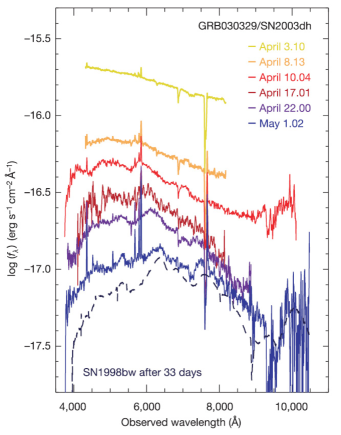
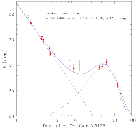
Figure 1.1: Left: Spectral evolution of the combined optical flux density of GRB 030329, the associated SN2003dh, and its host galaxy (colored lines) compared to the spectrum of SN1998bw (dashed line). Right: R-band light curve for GRB041006. A typical GRB power-law decay of the optical afterglow is shown as the dashed line and the SN1998bw light curve extended by a factor of 1.38 is shown as the dotted curve. Together they fit the observations. From Hjorth et al. (2003) (left) and Stanek et al. (2005) (right).

1.2 The general picture

After roughly 40 years with GRBs in the scientific spotlight, we are converging towards a working theory for GRBs.

There appears to be a general consensus in the scientific community about the fireball internal-external shock model, in which the gamma-ray burst and the subsequent afterglow radiation is created by dissipation of collisionless plasma shocks. Independent of the true nature of the progenitor, the extremely large amount of energy deposited in a very small volume inevitably creates a highly energetic outflow that will interact with the surrounding medium (Shemi and Piran, 1990).

For a detailed discussion, several good review papers exist (e.g., Fishman and Meegan 1995, Piran 1999, van Paradijs et al. 2000, Mészáros 2001, Mészáros 2002, Zhang et al. 2004, and Piran 2005b).

To explain the origin and variability of the prompt gamma emission, it was suggested that the progenitor may expel multiple plasma shells with different energies. The shells heat up in shocks when they overtake each other (Rees and Meszaros, 1994; Paczyński and Xu, 1994). At later times, an external shock forms as the ejecta blasts through the external medium. The external medium can either be the interstellar medium or a progenitor wind. This shock heats up the external plasma and creates the afterglow (Rees and Meszaros, 1992; Meszaros and Rees, 1993).

As the fireball expands into the external medium it sweeps up external matter and is expected to eventually approach the self similar Blandford-McKee solution (Blandford and McKee, 1976). This is a blast wave solution analogues to the non-relativistic Sedov-Taylor solution (Granot and Sari, 2002; Sari and Piran, 1995). For an extensive review on the GRB blast wave physics, see Piran (1999).

Rees and Meszaros (1992) and Meszaros and Rees (1993) suggested synchrotron radiation as the main radiation mechanism. The synchrotron radiation assumption naturally implied that the spectrum would soften and fade as a power law in time, and that an optical and radio afterglow would be present at later times (Paczyński and Rhoads, 1993; Katz, 1994). The radiation from both internal and external shocks is fairly well fitted by synchrotron and inverse Compton radiation from a high-energy non-thermal electron population in a strong magnetic field. Below (section 1.3 and 1.4) I discuss the non-thermal acceleration and the possible origin of the magnetic field.

Figure 1.2: The jet break of GRB 990510. The break is interpreted as the limit where the relativistic jet is decelerated enough so that the relativistic beaming angle ($~{}1/\Gamma$) becomes larger than the jet opening angle $\theta_{j}$. When this happens, the beaming angle covers an increasingly larger area outside the jet and the temporal decay will appear faster. From Harrison et al. (1999).

It is now well established that the relativistic gamma-ray burst ejecta are collimated. A collimated outflow is indeed a more compelling scenario since the required energy release from the progenitor is greatly reduced. If the emission were isotropic, the cosmological distances would imply that some bursts emit more than one solar mass in gamma rays. Such energies are hard to produce instantaneously in any stellar model. An observational fact that supports the collimation model is an achromatic break in the power law slope of the light curves. For many afterglows this happens days to weeks after the burst (Kulkarni et al., 1999; Harrison et al., 1999) (see Fig. 1.2). Such a break was suggested and interpreted as the limit where the relativistic jet is decelerated enough so that the relativistic beaming angle ($~{}1/\Gamma$) becomes larger than the jet opening angle $\theta_{j}$ (Rhoads, 1997, 1999; Panaitescu and Mészáros, 1999; Sari et al., 1999). When this happens, the beaming angle covers an increasingly larger area outside the jet and the temporal decay will appear faster.

One of the big unanswered questions concerns the jet structure. Calculating the energy budget for a burst requires crucial knowledge of the angular shape of the jet. The simplest structure is a jet where the internal energy, density and bulk Lorentz factor are constant throughout the jet cone (Rhoads, 1999; Sari et al., 1999). A more advanced model is the universal structured jet where the jet parameters vary smoothly with the angle measured from the jet symmetry axis (Lipunov et al., 2001; Rossi et al., 2002; Zhang and Mészáros, 2002). Simulations by Zhang et al. (2004) of the jet break-out from a massive Wolf-Rayet star show that the jet consists of at least two components (a highly relativistic thin jet and a less relativistic cocoon jet).

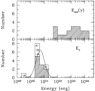
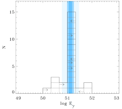
Figure 1.3: Correcting the total emitted gamma-ray energy corrected for beaming angle. From Frail et al. (2001) left and Bloom et al. (2003) (right).

Correcting for the jet geometry, the total required burst energy drops from $10^{47}\ \mathrm{J}$ to around $10^{44}\ \mathrm{J}$, not too far from the supernova output. More remarkably, in both the uniform structured jet and the universal structured jet model, the gamma-ray energy releases for many bursts are narrowly clustered around $5\times 10^{43}\ \mathrm{J}$ (Frail et al., 2001; Bloom et al., 2003) (see Fig. 1.3). In the uniform structured jet model, the different light curve break times are explained by different opening angles. The universal structured jet explains the break time spread by differences in the angle between the line of sight and the jet symmetry axis (Rossi et al., 2002; Zhang and Mészáros, 2002).

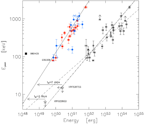
Figure 1.4: The Amati et al. (2002) and Ghirlanda et al. (2004) relations. The Amati relation links the total isotropic equivalent gamma-ray energy to the peak energy. The Ghirlanda relation (solid line) links the beaming corrected total energy to the $\nu F_{\nu}$ peak energy in the cosmological rest frame of the burst. From Ghirlanda et al. (2004).

Another striking correlation is the Amati correlation. Amati et al. (2002) found a correlation between the peak in $\nu F_{\nu}$ and the total isotropic equivalent burst energy. An even tighter correlation was found between the typical photon energy and the beaming corrected gamma-ray output during the burst (Ghirlanda et al., 2004) (see Fig. 1.4). These correlations have so far been purely empirical, with no viable physical explanation. Recently however, Ryde (2005) suggested a hybrid model consisting of a strong thermal component accompanied by a non-thermal component of similar strength. Ryde (2005) made fits of 25 strong bursts and compared the hybrid model to the commonly used Band function (Band et al., 1993). The result showed almost equally good fits for the two models except for ten of the burst where the hybrid model is marginally better.

In Ryde’s hybrid model, the peak of the burst is determined primarily by the temperature and is less sensitive on $\Gamma$. In this case, the Amati/Ghirlanda correlations have a natural explanation, since for a thermal emitter the luminosity and the temperature are correlated. Rees and Meszaros (2004) show that a correlation close to the observed one arises naturally under certain assumptions.

Thus, it would seem that GRBs are becoming excellent standard candles for probing the dark ages of the universe.

1.3 Particle acceleration in collisionless shocks

One of the key ingredients in generating what is believed to be non-thermal synchrotron radiation from GRB afterglows is a non-thermal, high-energetic electron population. Placing an ensemble of electrons with a power-law energy distribution function $dN(E)\propto E^{-p}dE$ in a homogenous magnetic field will result in a synchrotron radiation spectrum with a power-law segment $F(\nu)\propto\nu^{-(p-1)/2}$ (e.g. Landau and Lifshitz 1975 and Rybicki and Lightman 1979).

Many afterglow and Cosmic Ray models assume that electrons are accelerated in collisionless shocks by diffusive Fermi acceleration (Fermi, 1949). In first-order Fermi acceleration, the particles are accelerated as they repeatedly cross the shock transition jump. In the shock rest frame, the incoming upstream particles are stochastically deflected by a magnetic field as they pass the shock region. In this process, a fraction of the particles are kicked to higher energy. These high-energy particles then run into the upstream region and a fraction of the particles are reflected into the shock again for further acceleration. This iterative process continues in a competitive game between energy gain and escape of particles.

The theory of diffusive shock acceleration predicts that for non-relativistic shocks, the resulting particle distribution function converges to a power-law with the slope

$$p=\frac{v_{u}+2v_{d}}{v_{u}-v_{d}}\ \ \ \ \ \mathrm{or}\ \ \ \ \ s=\frac{3v_{u}}{v_{u}-v_{d}}$$ (1.1)

(e.g. Axford et al. 1977, Bell 1978 and Blandford and Ostriker 1978). Here $v_{u}$ and $v_{d}$ are the upstream and downstream plasma bulk velocities. The notation $s=p+2$ is more common in the literature of particle acceleration ($d^{3}N(p)/dp^{3}\propto p^{-s}$ where p is the particle momenta).

In the relativistic limit, the Fermi acceleration formalism becomes more complicated. The non-relativistic derivation is based on the diffusion equation (Kirk and Schneider, 1987), derived under the assumption that the particle distribution function is approximately isotropic in the local plasma rest frame. But for relativistic shocks, the bulk flow is comparable to the particle velocities and then the particle angular distribution function becomes highly anisotropic near the shock. In this case, strong magnetic fluctuations downstream of the shock are essential (Achterberg et al., 2001). Kirk and Schneider (1987) and Heavens and Drury (1988) investigated the relativistic problem and found the distribution slopes

$$p=\frac{R+2}{R-1}\ \ \ \ \ \mathrm{or}\ \ \ \ \ s=\frac{3R}{R-1},$$ (1.2)

where $R$ is the shock compression factor. Both analytical (Kirk et al., 2000) and Monte-Carlo (Bednarz and Ostrowski, 1998; Achterberg et al., 2001) find that $p$ converges at 2.23 for $\Gamma\to\infty$ ($\Gamma$ is here the bulk Lorentz factor).

The major force of relativistic first-order Fermi acceleration is that it predicts indices very close to the ones inferred from observations. Estimates from a number of GRB afterglows yield $p=2.2\pm 0.2$ (Waxman, 1997b; Berger et al., 2003). Good agreement and predictions are, however, not the same as a scientific proof. Afterglows exist that have a much larger variety in $p$. E.g. Campana et al. (2005) find $p=1.3$ in the very early afterglow. Here I emphasize some of the problems that the Fermi acceleration scenario in GRB afterglows is still facing:

Problem 1

It is very important to stress that Fermi acceleration in collisionless shocks is still not understood from first principles. The foundation of the acceleration mechanism is based on the test-particle approximation. It is assumed that the particles scatter on electromagnetic waves but the model does not self-consistently account for the generation of these waves. Nor does it account for the back-reaction that the high-energy particle distribution have on the electromagnetic field. Acceleration that results from currents and charge separation near the shock must be probed with a full kinetic approach (e.g. particle-in-cell codes). See section 1.3.1 and Chapter 5.

Problem 2

In all derivations of the relativistic Fermi acceleration mechanism, the downstream magnetic field is required to be strongly turbulent on scales smaller than the typical gyro-radius (e.g. Ostrowski and Bednarz 2002). This is, however, in conflict with the GRB afterglow synchrotron interpretation where the high-energy particles are expected to gyrate in circular orbits in a magnetic field with variation scale length much longer that the gyro-radii. Either the ansatz of strong downstream turbulence must be relaxed, with the result that the high-energy particle distribution function is not nearly as universal and possible not power-law at all (Ostrowski and Bednarz, 2002; Niemiec and Ostrowski, 2004; Baring, 2005). Or, the radiation model must be altered to include jitter radiation (Medvedev, 2000). See also Chapter 7.

Problem 3

Relativistic Fermi acceleration requires a pre-acceleration mechanism that injects electrons into the iterative acceleration process. The pre-acceleration mechanism is not well-known. How large a fraction of the electrons that are accelerated greatly affects our estimates of the total GRB energy (Eichler and Waxman, 2005). We define this fraction as $f$. Moreover, according to Baring and Braby (2004), agreeable synchrotron and/or inverse Compton fits are only attainable when the electron population has a significant non-thermal component. This is in disagreement with the Fermi process where electrons are injected from a dominant thermal pool. The lack of a dominant thermal pool also raises a question of how the electromagnetic turbulence is sustained in the shock-region.

Problem 4

This problem is connected to problem 3. In the closest and best studied mildly relativistic shock in the Crab Nebula, most of the electrons radiate below the expected injection energy and this means that $f\ll 1$ (Eichler and Waxman, 2005). The ”low” energy electrons have a power-law distribution spectrum $1.3\geq p\geq 1.1$ (Weiler and Panagia, 1978). This is much lower than what is expected from test particle simulations. The high-energy electrons, however, are more consistent with slope expected from first order Fermi acceleration $p\simeq 2.2$.

Problem 5

If the standard Fermi diffusive shock acceleration theory is correct, one expects an X-ray halo around the shock. This is because higher energy electrons are expected to diffuse further ahead of the shock, so the halo should become more extensive at X-ray wavelengths. Long et al. (2003) have investigated high resolution Chandra images of the close by Supernova remnant SN 1006. They fail to detect such a halo. Instead they see a sharp jump in emissivity at the shock. They conclude that either Fermi acceleration is absent in this shock, or some kind of shock instability must be operating in shocks that can create or amplify a magnetic field with a factor significantly larger than that given by the fluid compression, resulting in greater contrast between upstream and downstream emission (Long et al., 2003).

1.3.1 Particle acceleration in PIC simulations

Clearly, further advances in our understanding of particle acceleration in collisionless shocks require a full, self-consistent kinetic treatment. This may be provided by particle-in-cell (PIC) simulations (see Chapter 2). Unfortunately, PIC code simulations are very computationally demanding. Therefore, many PIC simulations up to date are one-dimensional. Here, I briefly review the state of particle acceleration in PIC code simulations.

One of the first reports of non-thermal acceleration in PIC simulations of relativistic collisionless plasma shocks came from Hoshino et al. (1992). In their (one-dimensional) simulations, plasma, carrying a magnetic field, is injected at the leftmost boundary. At the rightmost boundary, the plasma flow is reflected and thus collides with itself. In a plasma consisting purely of electron/positron pairs, they find that the acceleration is mainly thermal. When protons are present the positrons are strongly accelerated. The acceleration is driven by resonant absorbtion of magnetosonic waves, excited by energy dissipated from the gyrating ions. Hoshino et al. (1992) found that the positrons could be accelerated to a power-law distribution with slope $p=1.5-2.5$ and that the spectrum extended up to $\Gamma m_{i}c^{2}$. The reason why only positrons and not electrons are participating in the acceleration has to do with the polarization of the magnetosonic waves.

Another mechanism was examined with PIC simulations by Dieckmann et al. (2000, 2004). Based on theoretical work by Galeev A.A. (1995), Dieckmann et al. (2000, 2004) used PIC simulations of counter-streaming proton beams on a cold plasma background in a transverse magnetic field. They found traces of non-thermal particle acceleration up to mildly relativistic energies, offering an explanation to the injection problem. One should note, however, that their simulations were limited to one spatial dimension and the setup in itself is based on many assumptions about the initial conditions. It is not clear if the ion beam is injected on a quasi-neutral plasma background. If this is indeed the case, there is an excess of correlated positive charges in the simulations. This might trigger unrealistic instabilities. The size and duration of the simulations are rather limited and it would be interesting to see the same simulations carried out in three-dimensions.

A very well studied acceleration mechanism is the so called surfatron (Katsouleas and Dawson, 1983; Dawson et al., 1983). The surfatron is a mechanism in which a particle is accelerated while it is trapped by a propagating large-scale perpendicular electrostatic wave. The waves are driven via the Buneman instability that arises when electron and ion beams drift at different velocities (Buneman, 1958, 1959). The acceleration of particles by trapping in electrostatic waves has been simulated with PIC simulations by Hoshino and Shimada (2002) and Shimada and Hoshino (2004) and has been linked to phase space holes or loopholes (Schmitz et al., 2002) (see Fig. 1.5).

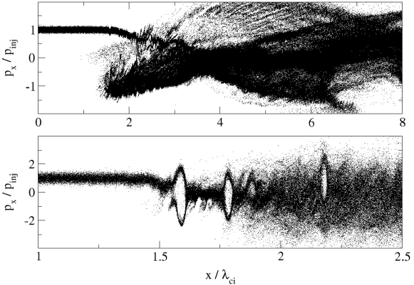
Figure 1.5: Phase space plot of ions (top panel) and electrons (bottom panel). The surfatron mechanism accelerate electrons by trapping in nonlinear wave modes linked to the existence of solitary electron phase space holes. The result is based on 1D PIC simulations. From Schmitz et al. (2002).

It should be noted that several independent simulations have indicated that the shock-fronts of collisionless plasma shocks, propagating in an ambient magnetic field, show great time variability (e.g. Lembege et al. (2004) and references therein). These simulations include both PIC simulations and hybrid simulations. In the latter, the ions are treated as particles and the electrons as a massless fluid. In one-dimensional PIC simulations by Lee et al. (2004) with parameters aimed at supernova shocks, the shock structure was found to be cyclically reforming on ion cyclotron timescales. In the reformation, Lee et al. (2004) found both electron loophole acceleration but also a suprathermal population of ions that could potentially explain the injection of high-energy ions into a Fermi acceleration scenario. The acceleration of electrons is interesting in the GRB context, and the acceleration of ions is interesting in regard to ultra high-energy cosmic rays.

All the simulations reviewed above have two things in common, 1) they are one-dimensional and 2) they assume that a rather strong transverse magnetic field is present. It would indeed be very interesting to explore whether effects such as electron trapping by electrostatic solitary waves will survive in three-dimensions, or if other effects become dominant, rendering the previous results artifacts of the one-dimensionality.

Specifically, I would like to express my reservation concerning the surfatron and loophole acceleration in relativistic collisionless shocks for the following reasons. The main driving mechanism is the excitation of electrostatic waves as a result of the Buneman two-stream instability. However, at relativistic velocities, the Weibel two-stream instability has a larger growth rate than the Buneman instability and will dominate the shock region (Califano, 2002). But the Weibel two-stream instability cannot be represented correctly in simulations with only one spatial dimension. Shimada and Hoshino (2004) have shown that the generation of loopholes is suppressed when the plasma frequency to cyclotron frequency ratio ($\omega_{pe}/\omega_{ce}\propto\sqrt{n}/B$) is less than 10 ($\omega_{pe}\equiv(nq^{2}/m_{e}\epsilon_{0})^{1/2}$ is the electron plasma frequency and $\omega_{ce}\equiv qB/m_{e}$ is the electron cyclotron frequency). Hededal and Nishikawa (2005) found in three-dimensional simulations that for $\omega_{pe}/\omega_{ce}>10$, the initial ordered ambient magnetic field becomes curled and even locally reversed because of the Weibel instability. Hededal and Nishikawa (2005) did find non-thermal acceleration, but for other reasons (see Chapter 5). So for $\omega_{pe}/\omega_{ce}<10$ the solitary electrostatic surfatron acceleration mechanism is suppressed and for $\omega_{pe}/\omega_{ce}>10$ the Weibel two-stream instability is present, which will distort the electrostatic wave generation. Finally, Hededal and Nishikawa (2005) found that in the interstellar medium where $\omega_{pe}/\omega_{ce}\simeq 1000$, the Weibel two-stream instability evolves unhindered, with no signs of loopholes or surfatrons (although Hededal and Nishikawa (2005) do point out the importance of larger simulations).

Clearly, the time has come for 2D or even 3D simulations to provide a more self-consistent explanation for the origin of the ambient magnetic field and non-thermal particle acceleration. Evidence from 3D PIC-simulations is gathering that suggests that particle acceleration and magnetic field generation are two highly connected features of collisionless plasma shocks (Frederiksen et al., 2002; Silva et al., 2003; Frederiksen et al., 2004; Nishikawa et al., 2003, 2005; Hededal et al., 2004; Hededal and Nishikawa, 2005). I save the discussion of these 3D PIC simulations of particle acceleration and the connection to field generation to section 1.4.1 below.

1.4 Magnetic fields in gamma-ray bursts

A second crucial ingredient in generation of radiation in GRB afterglows is the presence of a strong magnetic field. For a review on the role of magnetic fields in GRBs, see Piran (2005a).

The general working assumption is that the energy that resides in the magnetic field and in the non-thermal electrons may be parameterized by the equipartition parameters $\epsilon_{B}$ and $\epsilon_{e}$, and that the non-thermal electrons follow a power-law distribution with slope $p$ (where $\epsilon_{B}$ and $\epsilon_{e}$ are defined as the fractions of the total internal energy of the shock that are deposited in magnetic energy and kinetic energy of the electrons, respectively). It is generally assumed that these parameters are constant through the shock and even throughout the duration of the afterglow. The values are observationally determined by localizing certain characteristic break frequencies in the spectra. From low to high frequencies these are the synchrotron self-absorbtion frequency, the synchrotron frequency of the typical electron, and the self absorption frequency (Sari et al., 1998; Piran, 1999, 2005a, 2005b). Regarding the mangetic field, the typical value of the equipartition parameter in the afterglow is $\epsilon_{B}=0.0001-0.1$ (Waxman, 1997b; Wijers and Galama, 1999; Panaitescu and Kumar, 2002; Yost et al., 2003). This value may be translated to a magnetic field of the order of $10^{-4}\$T (1 G) in the afterglow shock. In the interstellar medium the typical magnetic field strength is of the order a few $10^{-10}$ T (few $\mu$G). According to the relativistic Rankine-Hugoniot plasma shock jump conditions (Taub, 1948), shock compression can only give a factor of $4\Gamma_{shock}$ and this is clearly far from enough to match the interpretations from observations (Gruzinov and Waxman, 1999). This leaves us with two possibilities for the origin of the magnetic field. One possibility is that the magnetic field is generated or amplified in the shock by microphysical instabilities and one is that the magnetic field is carried with the outflow from the progenitor. A magnetic field that originates from the progenitor and is frozen into the ejecta might account for the magnetic field in the internal shocks. But as the plasma shell expands, the magnetic field is diluted and dissipated to well below the anticipated values (e.g. Medvedev and Loeb 1999). Additionally, there exists a question of how to transport a magnetic from the ejecta and into the shocked ISM (all though theoretically it may happen via the Rayleigh-Taylor instability). Hence, the magnetic field responsible for the afterglow is most likely to be generated in situ in the shock.

Under collision of two relativistic plasma populations, the particle phase space is extremely anisotropic. Naively one could argue that in the absence of particle collisions, the two plasma populations would stream right through each other. The anisotropy is, however, unstable to several plasma instabilities, including the electrostatic Buneman two-stream instability and the electromagnetic Weibel two-stream instability. At relativistic shocks, the latter has the largest growth rate and will dominate (Califano, 2002; Hededal and Nishikawa, 2005). Gruzinov and Waxman (1999) and Medvedev and Loeb (1999) suggested that the Weibel two-stream instability could generate a strong magnetic field in the shock region. Since many of the results that I present in this thesis are connected to the Weibel two-stream instability, it is worthwhile to explain the nature of the instability in some detail. The following description is based on papers by Weibel (1959), Freid (1959), Medvedev and Loeb (1999), and Wiersma and Achterberg (2004).

Weibel (1959) suggested that if an isotropic plasma population is anisotropically perturbed, relaxation will lead to a growing transverse magnetic field, even in the absence of an external electromagnetic field. The same year, Freid (1959) gave a physical interpretation, where the anisotropic perturbation was described as an actual two-stream configuration. Since there will always be infinitesimal magnetic perturbations in a plasma, Fried suggested that deflection of the electrons (by the Lorentz force) in such a fluctuating magnetic field will create currents that can amplify the initial magnetic perturbation. Figure 1.6 shows a schematic drawing of this mechanism (Medvedev and Loeb, 1999). In the center of mass rest frame, two oppositely directed electron beams collide at $x=0$ (with bulk velocities $v_{1x}=-v_{e}$ and $v_{2x}=v_{e}$ so that the net current is zero). The ions are treated as a homogenous non-interacting background, to ensure charge neutrality. At x=0, a magnetic perturbation is initially present with $B_{z}=B_{0}\cos{ky}$. This perturbation deflects left streaming and right streaming electrons into anti-parallel currents with a distance comparable to the wavelength of the magnetic perturbation. According to Ampere’s law these currents represent a curl in the magnetic field. This curl amplifies the initial perturbation, which, in turn, collects even more electrons into the current channels. This positive feedback results in an instability where magnetic fluctuations grow with a rate $\sigma=\omega_{pe}v_{e}/c$ (Freid, 1959). Again, $\omega_{pe}$ is the electron plasma frequency defined above.

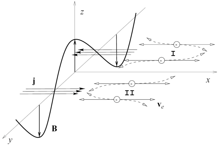
Figure 1.6: Schematic of the Weibel two-stream instability. Counter-streaming electrons are collected into opposite directed current channels by a magnetic perturbation. The current channels amplify the initial perturbation. From Medvedev and Loeb (1999).

The relativistic generalization is not trivial. The problem have been investigated by Yoon and Davidson (1987) who find the maximum growth rate to be $\sigma=\omega_{pe}/\Gamma^{1/2}$ where $\Gamma$ is the bulk relativistic Lorentz factor. The result can be understood intuitively by evaluating the non-relativistic expression in the limit where $v_{e}\to c$ and $\omega_{pe}\to(nq^{2}/\Gamma m_{e}\epsilon_{0})^{1/2}$.

Medvedev and Loeb (1999) estimated that the instability would saturate at $\epsilon_{B}\sim 10^{-5}-10^{-4}$ if only the electrons participate in the instability, and $\epsilon_{B}\leq 10^{-1}$ if also the ions take part in the instability. Wiersma and Achterberg (2004) found from a linear analysis that the two-stream instability in an electron-proton plasma shock has an early end where $\epsilon_{B}\leq m_{e}/m_{i}$ and that the wavelength of the most efficient mode for magnetic field generation equals the electron skin depth. Numerical simulations of the instability have shown that this limitation not true for the non-linear stage.

1.4.1 Magnetic field generation in PIC simulations

To investigate the non-linear stage of the Weibel two-stream instability, self-consistent kinetic particle-in-cell (PIC) simulations are necessary. In Chapter 2 I briefly describe the theory behind PIC codes with their advantages and disadvantages.

The first PIC simulations with direct focus on the Weibel instability in an astrophysical context were performed by Kazimura et al. (1998). They were interested in the plasma wind interaction in millisecond binary pulsars. In two-dimensional simulations of size $6.6\times 106.6$ electron skin depths, they investigated the collision of two mildly relativistic pair-plasma winds ($v_{0}=0.5c$). They found that up to five percent of the kinetic energy was converted into magnetic fields.

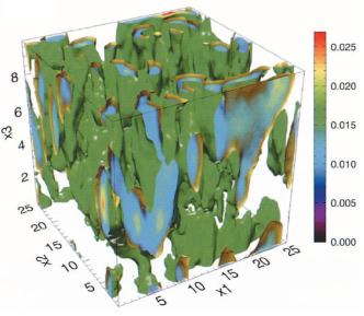
Figure 1.7: The structure of current channels generated by the Weibel two-stream instability under the collision of two pair-plasma shells (left panel). The corresponding amount of generated magnetic end electric field is close to equipartition (right panel). From Silva et al. (2003).

The collision of pair plasma shells was investigated with three-dimensional simulations by Silva et al. (2003). In a simulation box with size $25.6\times 25.6\times 10.0$ electron skin depths, they explored the collision of pair-plasma shells with relativistic Lorentz factors ranging from $\Gamma\sim 1$ to $\Gamma=10$. They found that the generated magnetic field reached maximum of $\epsilon_{B}\sim 0.1$ and afterward relaxed to $\epsilon_{B}\sim 0.0001-0.01$ (see Fig. 1.7). I emphasize that in these simulations the boundaries in the flow direction are periodic. It is not clear what this implies, but it can potentially introduce non-physical, stabilizing feed-back, since each current-filament is feeding itself.

Figure 1.8: The electron density (left panel) and current density (right panel). The arrows show the induced magnetic field. From Nishikawa et al. (2005).

Nishikawa et al. (2003) and Nishikawa et al. (2005) have performed three-dimensional simulations of both pair-plasma and electron-proton shocks in a numerical box with size $17.7\times 17.7\times 66.7$ electron skin depths (corresponding to $4\times 4\times 14.9$ ion skin depths for ion-electron mass ratio $m_{i}/m_{e}=20$) (see Fig. 1.8). With these simulations they were able to follow primarily the linear stage of the instability at the front of the shock ramp (the ambient and jet electron populations are not thermalized to a single population in the simulations). With the simulations Nishikawa et al. confirmed the growth rate predicted by Weibel (1959), Freid (1959) and Medvedev and Loeb (1999). They also found signs of electron acceleration connected to the instability, but whether the nature of this acceleration is non-thermal or merely a thermalization is not clear.

Figure 1.9: The left hand side panel shows the longitudinal electron current density through a transverse cut early in the shock. The right hand side panel shows the ion current deeper in the shock. The arrows represent the transverse magnetic field. From Frederiksen et al. (2004).

Frederiksen et al. (2002, 2004) and Hededal et al. (2004) have investigated the non-linear evolution the two-stream instability in electron-proton shocks. Details are given in Chapter 3 and Chapter 6 of this thesis. Here I give a short summary. Frederiksen et al. (2004) performed simulations of electron-proton shocks with $\Gamma=3$. The size of the simulation box was $40\times 40\times 160$ electron skin depths (corresponding to $10\times 10\times 40$ ion skin depths for ion-electron mass ratio $m_{i}/m_{e}=16$). The results of these simulations showed how Weibel generated ion current filaments were collected into increasingly larger patterns in the non-linear stage. This phenomenon has been investigated both analytically and numerically in great details by Medvedev (2005). Frederiksen et al. (2004) also found that the ion current filaments are partially Debye shielded by shock-heated electrons. The electrons thus act as insulators for the ion-current filaments, making these rather robust (see Fig. 1.9). The results showed that a magnetic field was generated ($\epsilon_{B}\sim 0.05$) and sustained for many ion skin depths. This answers a concern raised by Gruzinov (1999), who estimated that the magnetic field can only be sustained for roughly one electron skin depth.

Figure 1.10: The high-energy electrons (red colored dots) are found where the ion-current filaments are strongest (blue colors). From Hededal et al. (2004).

Hededal et al. (2004) found that not only can the Weibel two-stream instability account the generation of a strong magnetic field, but it appears that non-thermal electron acceleration is a natural consequence of the process. They found that high-energy electrons are spatially connected to the ion current filaments (see Fig. 1.10 and Chapter 6). The acceleration and deceleration of electrons is local and instantaneous. This is in contrast to the recursive process of Fermi acceleration.

1.5 Summary and Thesis Outline

The radiation from GRB afterglows is produced in relativistic, collisionless plasma shocks by two key ingredients, namely 1) a population of highly energetic, non-thermal electrons and 2) a strong electromagnetic field. All our knowledge of GRBs are based on this radiation. Nevertheless, the questions of how the electrons are accelerated, and what the exact generation mechanism and nature of the electromagnetic field in the shock is, have not yet been answered in a self-consistent way and are still open questions.

Even though magnetic field generation by the Weibel two-stream instability seems necessary (and also unavoidable) in collisionless shocks in GRB afterglows, it have not yet been possible to verify or discard it from observations. One way to investigate on the magnetic morphology in these shocks is to measure the polarization of afterglows, although this also relies heavily on the jet structure. Lazzati et al. (2004) found that polarization of GRB 020813 is not very well fitted with a homogenous jet with shock generated field. I stress that to draw any conclusions from observations about the magnetic field and particle acceleration, it is vital to have a firm understanding of collisionless shocks, and the generation of radiation in these.

It is the goal of this thesis to shed light on the microphysics of collisionless plasma shocks, mainly in the context of gamma-ray burst afterglows. Using a particle-in-cell code that works from first principles, the aim is to obtain insight in, and explain the origin of, the magnetic field in these shocks, the nature of the field, and how it may influence the radiation emitted from GRB afterglows.

The thesis is divided into 9 chapters:

• In Chapter 2 I describe the particle-in-cell code that have been used and how radiative cooling has been implemented.

• Chapter 3 presents the results of simulations of the non-linear evolution of the Weibel two-stream instability. This chapter is based on the paper by Frederiksen, Hededal, Haugbølle and Nordlund (2004).

• In Chapter 4 I compare two- and three-dimensional simulations, and present results of large-scale shock simulations. This work has not yet been submitted to a scientific journal.

• Chapter 5 investigates the microphysics of collisionless plasma shocks in the presence of an ambient magnetic field. This chapter is based on the paper by Hededal and Nishikawa (2005).

• In Chapter 6 I present a new particle acceleration mechanism that differs from Fermi acceleration. This paper is based on the paper by Hededal, Haugbølle, Frederiksen and Nordlund (2004).

• In Chapter 7 I describe the development and test of a new and powerful numerical tool, which may be used to create radiation spectra directly from PIC simulations. This work has not yet been submitted to a scientific journal.

• Chapter 8 describes the foundations of a next generation particle-in-cell code that includes photons and various scattering processes. The chapter includes some preliminary test results with Compton scattering.

• In Chapter 9 I collect all the pieces from the thesis in a summary and conclusions. Here I also discuss the future of the line of work that I have presented in this thesis.

Chapter 2 The Particle–In–Cell code

In this Chapter I briefly describe the kinetic particle-in-cell code, and justify why it is important compared to a fluid description. I also discuss some of the limitations of a kinetic numerical description. Finally, I describe in some detail the derivation, implementation and testing of a radiative cooling mechanism in the code.

2.1 Kinetic or fluid description of collisionless shocks.

The mean free path for a $90^{\circ}$ Coulomb deflection of an electron moving with relativistic momentum $\Gamma v_{e}m_{e}$ in a plasma (with density $n$) is

$$\lambda_{c}=\frac{1}{n\sigma_{c}}=\frac{16\pi\epsilon_{0}^{2}\sqrt{2}\gamma^{2}m_{e}^{2}v_{e}^{4}}{ne^{4}}.$$ (2.1)

See Appendix A for details. For a relativistic GRB jet that expands into the interstellar medium (ISM), we may use this expression to estimate the typical mean free path for Coulomb collisions between the jet and ISM particles. With an ISM density $n\simeq 10^{6}\mathrm{m}^{-3}$ and a jet bulk Lorentz factor $\gamma=5$ ($v\simeq c$), the mean free path for Coulomb collisions is $10^{24}\mathrm{m}$. This is of the order of a billion times the expected size of the fireball. Thus one might naively expect a relativistic jet to expand unhindered through the ISM. This is however, in direct contrast with observations, where gamma-ray burst afterglows are described by synchrotron emission from decelerating relativistic shells that collides with, and heats, an external medium. Lack of interactions would pose serious problems in explaining the particle acceleration and origin of the magnetic field, which is needed to produce the observed synchrotron radiation (e.g. Waxman 1997a and Sari et al. 1998). Not surprisingly, the collisional interaction agent must be found in the microphysical processes at play between particles and electromagnetic fields (Sagdeev, 1966).

From this discussion it is clear that a treatment of the jet/ISM interaction needs to be established. For this purpose we need a theoretical framework. The use of the Magneto-Hydro-Dynamic equations (MHD) in this context is discarded by several arguments:

• The low collision rate cannot provide the equilibration of ion and electron energies sufficiently fast for the plasma to behave as a fluid. This is the case even for the ”low energy” shocks associated with supernova remnants (Draine and McKee, 1993; Vink, 2004). Observations are consistent with an energetically important population of accelerated particles superimposed on a low energy background population Gruzinov (2001).

• MHD shocks are stable and do not generate magnetic fields. In MHD shocks, magnetic fields are only compressed, with a resulting field strength that is orders of magnitudes smaller than what is required by the synchrotron model of GRB afterglows (Gruzinov, 2001).

2.2 From first principles

The solutions that we are seeking fall into the kinetic and highly non-linear regime of plasma physics. In this case, we need to work from first principles, by solving the Maxwell equations with source terms for the electromagnetic fields, together with the relativistic equation of motion for charged particles

$$\nabla\cdot\mbox{\boldmath$\mathrm{E}$}&=\frac{\rho}{\epsilon_{0}}\\ \nabla\times\mbox{\boldmath$\mathrm{B}$}-\frac{d\mbox{\boldmath$\mathrm{E}$}}{c^{2}dt}=\mu_{0}\mbox{\boldmath$\mathrm{J}$}\\ -\nabla\times\mbox{\boldmath$\mathrm{E}$}=\frac{d\mbox{\boldmath$\mathrm{B}$}}{dt}\\ \nabla\cdot\mbox{\boldmath$\mathrm{B}$}=0$$ (2.2)

and

$$m\frac{d(\gamma\mbox{\boldmath$\mathrm{v}$})}{dt}=q(\mbox{\boldmath$\mathrm{E}$}+\mbox{\boldmath$\mathrm{v}$}\times\mbox{\boldmath$\mathrm{B}$}).$$ (2.3)

Here $\epsilon_{0}$ and $\mu_{0}$ are the constants of electric permittivity and magnetic permeability of vacuum, with $c^{2}\mu_{0}\epsilon_{0}=1$. $m$ and $q$ are the mass and charge of a particle of a given species, $\mathrm{v}$ is the velocity vector and $\gamma\equiv(1-v^{2}/c^{2})^{-1/2}$ is the relativistic Lorentz factor. The source terms, $\mathrm{J}$ and $\rho$, in the Maxwell equations are determined by the particles in the simulations.

We wish to find a general solution to the coupled differential equations of Eq. 2.2 and Eq. 2.3. For a given set of initial/boundary conditions with, say, $10^{25}$ particles, this is not analytically possible. Numerically, however, solving a scaled-down version of the same problem is doable, with particle-in-cell (PIC) codes (e.g. Birdsall and Langdon 1991). Much like in a real plasma, a PIC code integrates the trajectories of a large number of charged particles in both external and self-induced electromagnetic fields. Some limitations exist in this approach. Some of the main differences between a PIC simulated plasma and a real plasma are:

• The number densities of real space are many orders of magnitudes larger than what can be fitted in a computer: A $10\times 10\times 10\ \mathrm{m}^{3}$ cube of the ISM contains approximately $10^{9}$ charged particles, and even this is barely computational affordable today. Therefore, in the simulations, each particle is a macro-particle that represents a large number of real-plasma charges. Each macro-particle keeps the same charge to mass ratio as the individual particles it is made of.

• Even though continuous in space and momentum space, the particles positions are discretized in time.

• The electromagnetic fields are discretized is space as well as time. The Maxwell equations are integrated on a fixed numerical grid and the interactions with the particles in a given grid cell are done via interpolations from grid to particle positions and vice versa (hence the name particle-in-cell). The electromagnetic field components and source-terms are staggered and distributed on a 3D Yee lattice (Yee, 1966). This gives a resolution improvement that corresponds to a factor 16 in computing time (Fig. 2.1).

• Many plasma processes evolve on time scales that are proportional to the plasma frequency $\tau\propto\omega_{p}^{-1}$ and on length scales that are proportional to the skin depth $\delta\equiv c/\omega_{p}$. Therefore, a large spatial and temporal span exists in plasma processes that are dominated by respectively ions and electrons. To comply with the limitations in computational resources it is convenient to compress the dynamical ranges by reducing the ion (proton) to electron mass ratio $m_{i}/m_{e}$ from the real value (1836) to 15-30. This is clearly an approximation but we have performed tests that have shown that the results show good convergence for mass ratios above 15-30. For lower mass ratio, the results are still qualitatively correct.

• The maximum temporal and spatial scale-lengths in PIC simulations are limited because it is important to resolve microphysical plasma oscillations. Since the electron plasma frequency $\omega_{pe}$ is often the limiting factor, we normalize time with respect to the oscillation period $\omega_{pe}^{-1}$ and the space with respect to the electron skin depth $c/w_{pe}$. The plasma frequency is defined as $\omega_{pe}\equiv(n_{e}q^{2}/m_{e}\epsilon_{0})^{-1/2}$, and thus the plasma density $n_{e}$ determines the re-scaling.

Despite these constraints, the PIC code representation of a plasma is far more fundamental than the MHD approximation. Still, PIC simulations are computationally challenging and fully three-dimensional experiments have only become practically possible within the last few years.

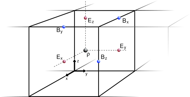
Figure 2.1: The staggered mesh. In a grid-cell, the particle densities are cell centered, the electric field and current source terms are face centered and the magnetic field components are edge centered. Distributing the field variables on a staggered mesh gives a factor 2 increase in resolution. In 3+1 dimensions this is a factor 16 in computing time.

The PIC-code implementation I use is based on a non-relativistic code developed by Dr. Michael Hesse. The code was initially developed for simulating reconnection topologies in the context of space weather (Hesse et al., 1999). The code was later made relativistic by Frederiksen (2002) as part of a masters project. Since then it has been used mainly for numerical plasma shock experiments related to GRB afterglows (Frederiksen et al., 2002, 2004; Hededal et al., 2004; Hededal and Nishikawa, 2005). As part of the current PhD project, radiative cooling has recently been included to the code. This is important for investigation of particle acceleration and generation of radiative spectra. A new PIC code, which includes photons and several scattering mechanisms, is under development (see Chapter 8).

2.3 Cooling of an accelerated charge

In this section I derive and describe the implementation of radiative cooling in the PIC-code. Radiative cooling is essential for highly relativistic particle dynamics and especially for experiments aimed at investigating particle acceleration. Before I describe the derivation and implementation an expression for the energy radiated from an accelerated charged particle into the PIC-code, I briefly revive the concept of retarded time and space.

2.3.1 Retarded time and position

Let a particle be in the position $\mbox{\boldmath$\mathrm{r}$}_{0}(t)$ at time $t$ (Fig. 2.2). At the same time, we observe the electric field from the particle in the position $\mathrm{r}$. However, because of the finite propagation velocity of light, we observe the particle at an earlier position $\mbox{\boldmath$\mathrm{r}$}_{0}(t^{\prime})$ where it was at the retarded time $t^{\prime}=t-\delta t^{\prime}=t-R(t^{\prime})/c$. Here $R(t^{\prime})=\left|\mbox{\boldmath$\mathrm{r}$}-\mbox{\boldmath$\mathrm{r}$}_{0}(t^{\prime})\right|$ is the distance from the charge (at the retarded time $t^{\prime}$) to the observer point.

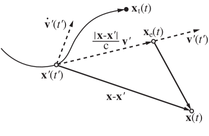
Figure 2.2: Definition of the retardation of a particles position. From an observers point $\mathrm{r}$ we see the particle at the position $\mbox{\boldmath$\mathrm{r}$}_{0}(t^{\prime})$ where it was at the retarded time.

2.3.2 Radiated power

To skip a trivial, but rather long derivation, we adopt the expression from Jackson (1999) for the retarded electric field from a charged particle moving with instant velocity $\mathrm{\beta}$ under acceleration $\dot{\mathrm{\beta}}$,

$$\mbox{\boldmath$\mathrm{E}$}=\underbrace{\frac{q}{4\pi\epsilon_{0}}\left[\frac{\mbox{\boldmath$\mathrm{n}$}-\mbox{\boldmath$\mathrm{\beta}$}}{\gamma^{2}\left(1-\mbox{\boldmath$\mathrm{n\cdot\beta}$}\right)^{3}R^{2}}\right]_{\mathrm{ret}}}_{\mathrm{velocity\ field}}+\underbrace{\frac{q}{4\pi\epsilon_{0}c}\left[\frac{\mbox{\boldmath$\mathrm{n}$}\times\{(\mbox{\boldmath$\mathrm{n}$}-\mbox{\boldmath$\mathrm{\beta}$})\times\mbox{\boldmath$\dot{\mathrm{\beta}}$}\}}{\left(1-\mbox{\boldmath$\mathrm{n\cdot\beta}$}\right)^{3}R}\right]_{\mathrm{ret}}}_{\mathrm{acceleration\ field}}.$$ (2.4)

Here, $\mbox{\boldmath$\mathrm{n}$}\equiv\mbox{\boldmath$\mathrm{R}$}(t^{\prime})/\left|\mbox{\boldmath$\mathrm{R}$}(t^{\prime})\right|$ is a unit vector that points from the particles retarded position towards the observer. The first term on the right hand side, containing the velocity field, is the Coulomb field from a charge moving without influence from external forces. The second term is a correction term that arises if the charge is subject to acceleration. Since the velocity-dependent field is falling of as $R^{-2}$ while the acceleration-dependent field falls off as $R^{-1}$, the latter becomes dominant when observing the charge at large distances ($R\gg 1$). This term is therefore often referred to as the radiation term. The corresponding magnetic field is given by

$$\mbox{\boldmath$\mathrm{B}$}=\left[\frac{\mbox{\boldmath$\mathrm{n}$}\times\mbox{\boldmath$\mathrm{E}$}}{c}\right]_{\mathrm{ret}}$$ (2.5)

.

The energy $W$ per unit area $dA$ per unit time $dt$ that is radiated from the accelerated particle is given by the Poynting flux $\mathrm{S}$

$$\mbox{\boldmath$\mathrm{S}$}\equiv\frac{d^{2}W}{dtdA}=\frac{\mbox{\boldmath$\mathrm{E}$}\times\mbox{\boldmath$\mathrm{B}$}}{\mu_{0}}=\frac{\left|E\right|^{2}}{\mu_{0}c}\mbox{\boldmath$\mathrm{n}$}$$ (2.6)

from which we define the energy per unit time, received through a unit solid angle element $d\Omega$ about $\mathrm{n}$

$$\frac{dP(t)}{d\Omega}=R^{2}\left[\mbox{\boldmath$\mathrm{S\cdot n}$}\right]_{\mathrm{ret}}.$$ (2.7)

A note of caution must be added here. The Poynting vector is related to the observer time $t$ but we are interested in the radiated power measured at the particle’s retarded time $t^{\prime}$. Thus, to get the total emitted power we multiply with the correction term $dt/dt^{\prime}$ (see Chapter 7 for details)

$$\frac{dP_{rad}}{d\Omega} = R^{2}\left(\mbox{\boldmath$\mathrm{S\cdot n}$}\right)\frac{dt}{dt^{\prime}}=R^{2}\mbox{\boldmath$\mathrm{S\cdot n}$}\left(1-\mbox{\boldmath$\mathrm{n\cdot\beta}$}\right)$$ (2.8)

$$= \frac{\mu_{0}q^{2}c}{16\pi^{2}}\frac{\left[\mbox{\boldmath$\mathrm{n}$}\times\left\{\left(\mbox{\boldmath$\mathrm{n}$}-\mbox{\boldmath$\mathrm{\beta}$}\right)\times\mbox{\boldmath$\dot{\mathrm{\beta}}$}\right\}\right]^{2}}{\left(1-\mbox{\boldmath$\mathrm{n\cdot\beta}$}\right)^{5}}.$$

Rather tedious vector algebra and integration over all directions $\mathrm{n}$ through the solid angle $d\Omega$ gives us the total power radiated by the particle in a time interval $dt^{\prime}$ (see Appendix B for details)

$$P_{rad}&=\frac{\mu_{0}q^{2}c}{6\pi}\gamma^{4}\left(\dot{\beta}^{2}+\gamma^{2}|\mbox{\boldmath$\mathrm{\beta\cdot\dot{\beta}}$}|^{2}\right)\\ =\frac{\mu_{0}q^{2}c}{6\pi}\gamma^{6}\dot{\beta}^{2}\left(1-\beta^{2}\sin^{2}\theta\right),$$ (2.9)

where $\theta$ is the angle between the particles velocity vector $\mathrm{\beta}$ and its acceleration vector $\dot{\mathrm{\beta}}$. When $\sin\theta=1\Leftrightarrow\mbox{\boldmath$\mathrm{\beta\perp\dot{\beta}}$}$, we recognize the solution for synchrotron radiation (magnetic bremsstrahlung). In the other limit, $\sin\theta=0\Leftrightarrow\mbox{\boldmath$\mathrm{\beta\parallel\dot{\beta}}$}$, we recover the result for bremsstrahlung. The results above may be found in many textbooks (Landau and Lifshitz, 1975; Jackson, 1999; Rybicki and Lightman, 1979).

In Chapter 7 we deal with radiation from relativistic particles in more details.

2.3.3 Implementing the radiative cooling

Before implementing Eq. 2.9 into the PIC-code, it is fruitful to derive the expression for a particles energy as it looses momentum to radiation.

From energy conservation we demand that the energy radiated from a particle must equally correspond to a loss in the particles kinetic energy $E_{kin}=mc^{2}(\gamma-1)$

$$\frac{dE_{kin}}{dt} = -P_{rad}$$

$$\Rightarrow\frac{d\gamma(t)}{dt} = -\frac{\mu_{0}q^{2}}{6\pi mc}\gamma^{6}\left(\dot{\beta}^{2}\left(1-\beta^{2}\right)+|\mbox{\boldmath$\mathrm{\beta\cdot\dot{\beta}}$}|^{2}\right),$$ (2.10)

which is the relativistic counterpart to the Larmor formula for radiated power. In order to continue we need an expression for $\dot{\mathrm{\beta}}$. The only force acting on the particle is the Lorentz force (we deal with the radiation reaction force in Section 2.3.4)

$$m\frac{d(\gamma\mbox{\boldmath$\mathrm{v}$})}{dt} = q(\mbox{\boldmath$\mathrm{E}$}+\mbox{\boldmath$\mathrm{v}$}\times\mbox{\boldmath$\mathrm{B}$})$$ (2.11)

$$\Rightarrow\gamma\frac{d\mbox{\boldmath$\mathrm{v}$}}{dt}+\frac{\mbox{\boldmath$\mathrm{v}$}\gamma^{3}}{c^{2}}\left(\mbox{\boldmath$\mathrm{v\cdot}$}\frac{d\mbox{\boldmath$\mathrm{v}$}}{dt}\right) = \frac{q}{m}(\mbox{\boldmath$\mathrm{E}$}+\mbox{\boldmath$\mathrm{v}$}\times\mbox{\boldmath$\mathrm{B}$}).$$ (2.12)

Here we have expanded the right hand side and used the relation

$$\frac{d\gamma}{dt}=\frac{d(1-\mbox{\boldmath$\mathrm{\beta\cdot\beta}$})^{-1/2}}{dt}=\frac{\gamma^{3}}{c^{2}}\mbox{\boldmath$\mathrm{v\cdot}$}\frac{d\mbox{\boldmath$\mathrm{v}$}}{dt}.$$ (2.13)

Unfortunately, we cannot provide a general solution to Eq. 2.10 and Eq. 2.12. We may, however, simplify the equation system by looking at a particle moving with $\gamma(t=0)=\gamma_{0}$ at an angle $\alpha$ to a homogeneous magnetic field ($\mbox{\boldmath$\mathrm{E}$}=0$). In this case, the Lorentz force is always perpendicular to the velocity vector and the term $\mathrm{v\cdot}$$\dot{\mathrm{v}}$ vanishes. Equation 2.10 and Eq. 2.12 then reduce to

$$\frac{d\gamma(t)}{dt}=\frac{\mu_{0}q^{4}}{6\pi m^{3}c}\sin^{2}(\alpha)B^{2}(\gamma^{2}(t)-1),$$ (2.14)

where we have used that $v^{2}(t)=c^{2}(1-\gamma^{-2}(t))$. This differential equation has the formal solution

$$\gamma(t)=\frac{2(\gamma_{0}-1)}{(\gamma_{0}+1)\exp\left[{\frac{\mu_{0}q^{4}}{3\pi m^{3}c}\sin^{2}(\alpha)B^{2}t}\right]-\gamma_{0}+1}.$$ (2.15)

If we in Eq. 2.14 assume that $\gamma\gg 1\Rightarrow v\sim c$, the solution becomes simpler, but less valid for low $\gamma$ (see fig. 2.3)

$$\gamma(t)=\frac{\gamma_{0}}{1+\frac{\mu_{0}q^{4}}{6\pi m^{3}c}\sin^{2}(\alpha)B^{2}\gamma_{0}t}.$$ (2.16)

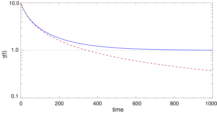
Figure 2.3: The two versions of $\gamma(t)$ – Eq. 2.15 and Eq. 2.16 – compared. The main difference is that in deriving Eq. 2.16 $v\sim c$ was assumed instead of the correct $v=c\sqrt{1-\gamma^{-2}}$ in Eq. 2.15. Thus, Eq. 2.16 becomes incorrect as $\gamma(t)\to 1$. The units on the time axis is given in terms of the initial orbital period.

In Section 2.3.4 I describe the implementation of the radiative damping from Eq. 2.9 into the PIC-code and find good agreement with Eq. 2.15.

Eq. 2.16 gives us an indication of when momentum losses to radiation becomes an important issue. If a physical process of interest occurs over a time span $T$, radiation may be neglected whenever

$$\kappa T\ll 1,$$ (2.17)

where

$$\kappa\equiv\frac{\mu_{0}q^{4}}{6\pi m^{3}c}\sin^{2}(\alpha)B^{2}\gamma_{0}.$$ (2.18)

We may also estimate the time $t_{1/2}$ it takes for a particle to loose half of its energy

$$mc^{2}(\gamma(t_{1/2})-1)=1/2mc^{2}(\gamma_{0}-1)$$

$$\Rightarrow t_{1/2}=\frac{6\pi m^{3}c}{\mu_{0}q^{4}B^{2}\gamma_{0}}\frac{\gamma_{0}-1}{\gamma_{0}+2}\ \mathop{\longrightarrow}_{\gamma_{0}\gg 1}\ \frac{6\pi m^{3}c}{\mu_{0}q^{4}B^{2}\gamma_{0}}.$$ (2.19)

2.3.4 Implementing the reaction force

When a particle emits radiation, it looses both energy and momentum to the emitted photons. Thus, in theory, we need to add an extra force term in Eq. 2.12. However, as stated by Jackson (1999) ”a complete satisfactory classical treatment of the reactive effects of radiation does not exist” (and it is noteworthy that Jackson only discuss the issue in the very last Chapter). One approach is the Abraham-Lorentz equation of motion

$$m\left(\frac{d(\gamma\mbox{\boldmath$\mathrm{v}$})}{dt}-\frac{d^{2}(\gamma\mbox{\boldmath$\mathrm{v}$})}{dt^{2}}\right)=\mbox{\boldmath$\mathrm{F}$}_{\mathrm{L}orentz},$$ (2.20)

but this solution is limited to periodic motions and have runaway solutions. A consistent, but rather extensive, implementation of the reaction force in a PIC code have been described by Noguchi et al. (2004).

Instead we derive a more empirical solution to the problem that is suitable for a numerical implementation.

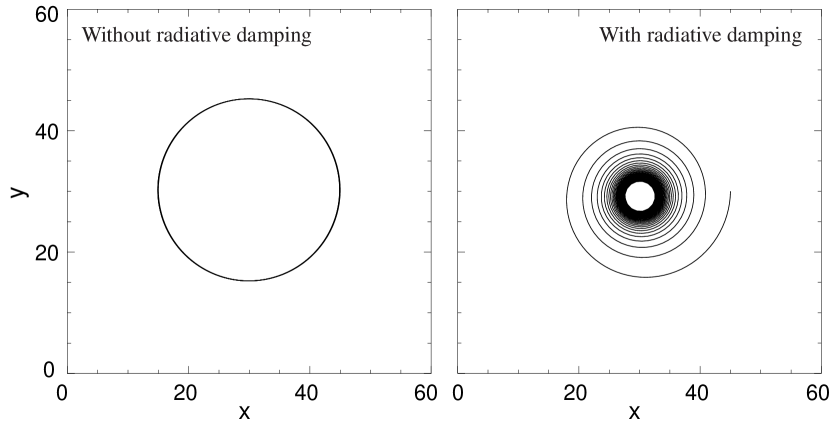
Figure 2.4: The trajectory of a relativistic particle in a transverse homogeneous magnetic field. The particles motion is integrated by the PIC code. The left panel shows the orbit without damping whereas the right panel shows the orbit of the particle as it looses momentum to radiation according to Eq. 2.23. Initially $\gamma_{0}=60$, $\kappa=0.005$ and the orbit is integrated over over the time interval $T=[0,1000]$.

We recall the expression for the particles kinetic energy lost to radiation

$$mc^{2}\frac{d(\gamma(t)-1)}{dt}=-P_{rad}.$$ (2.21)

We are looking for a way to modify the particles momentum vector $\mbox{\boldmath$\mathrm{u}$}=\gamma\mbox{\boldmath$\mathrm{v}$}$ that we may implement in the PIC-code. We allow ourself to make a discrete representation of Eq. 2.21

$$\frac{\tilde{\gamma}-\gamma}{\Delta t} = -\frac{P_{rad}}{mc^{2}}$$

$$\Rightarrow\tilde{\gamma} = \gamma-\frac{P_{rad}}{mc^{2}}\Delta t,$$ (2.22)

where $\gamma$ is the particle Lorentz factor from the code and $\tilde{\gamma}$ is the radiation corrected Lorentz factor. The corresponding radiation corrected momentum is $|\tilde{\mbox{\boldmath$\mathrm{u}$}}|=c\sqrt{\tilde{\gamma}^{2}+1}$.

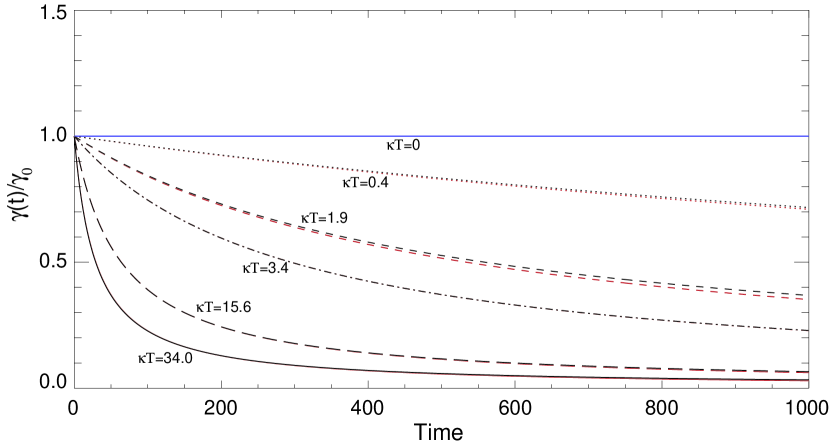
Figure 2.5: A comparison between cooling times in the theoretical approach of Eq. 2.15 (red lines) and the PIC-code implementation of Eq. 2.23 (black lines). The small discrepancies between the two approaches are mainly caused by numerical integration inaccuracy. The time is in arbitrary units.

We know that in an observers frame, the radiation from a relativistic particle is concentrated around the direction of its velocity vector (e.g. Landau and Lifshitz 1975). Therefore, we can make the assumption that the radiation reaction force is directed opposite to the momentum vector. In this case, the change in momentum occurs only along the momentum vector $\mathrm{u}$ and we have

$$\frac{\tilde{\mbox{\boldmath$\mathrm{u}$}}}{|\tilde{\mbox{\boldmath$\mathrm{u}$}}|} = \frac{\mbox{\boldmath$\mathrm{u}$}}{|\mbox{\boldmath$\mathrm{u}$}|}$$

$$\Rightarrow\tilde{\mbox{\boldmath$\mathrm{u}$}} = \mbox{\boldmath$\mathrm{u}$}\frac{|\tilde{\mbox{\boldmath$\mathrm{u}$}}|}{|\mbox{\boldmath$\mathrm{u}$}|}=\mbox{\boldmath$\mathrm{u}$}\frac{\sqrt{[\gamma-P_{rad}\Delta t/(mc^{2})]^{2}+1}}{\sqrt{\gamma^{2}+1}},$$ (2.23)

where $P_{rad}$ is given by Eq. 2.9. We have implemented Eq. 2.23 in the PIC code. To verify the correctness of the method, we test against the result from the analytical approach, Eq. 2.15. We make a simulation run with $\mbox{\boldmath$\mathrm{E}$}=0$ and a homogeneous magnetic field $\mathrm{B}$. A single particle is setup with a given velocity perpendicular to the magnetic field ($\sin^{2}\alpha=1$). The integrated path of the particle may be seen in Fig. 2.4. The figure shows that as the particle cools to lower gamma it approaches a state where cooling becomes negligible and the orbit becomes semi stable ($\kappa T\ll 1$).

A comparison of the PIC-code cooling rate against Eq. 2.15 may be found Fig. 2.5. Five different combinations of $\gamma_{0}$ and $B_{0}$ has been tested. Good agreement is found between the two approaches. The minor discrepancies that do appear are mainly caused by integrated interpolation errors in the second order scheme used in the PIC-code.

Chapter 3 The Weibel two-stream instability

In this chapter I present results from three-dimensional particle simulations of collisionless shock formation, with relativistic counter-streaming ion-electron plasmas (Frederiksen et al., 2004). Particles are followed over many skin depths downstream of the shock. Open boundaries allow the experiments to be continued for several particle crossing times. The experiments confirm the generation of strong magnetic and electric fields by a Weibel-like kinetic streaming instability, and demonstrate that the electromagnetic fields propagate far downstream of the shock. The magnetic fields are predominantly transversal, and are associated with merging ion current channels. The total magnetic energy grows as the ion channels merge, and as the magnetic field patterns propagate down stream. The electron populations are quickly thermalized, while the ion populations retain distinct bulk speeds in shielded ion channels and thermalize much more slowly. The results help us to reveal processes of importance in collisionless shocks, and may help to explain the origin of the magnetic fields responsible for afterglow synchrotron/jitter radiation from Gamma-Ray Bursts.

3.1 Introduction

The existence of a strong magnetic field in the shocked external medium is required in order to explain the observed radiation in Gamma-Ray Burst afterglows as synchrotron radiation (e.g. Panaitescu and Kumar, 2002). Nearly collisionless shocks, with synchrotron-type radiation present, are also common in many other astrophysical contexts, such as in super-nova shocks, and in jets from active galactic nuclei. At least in the context of Gamma-Ray Burst afterglows the observed synchrotron radiation requires the presence of a stronger magnetic field than can easily be explained by just compression of a magnetic field already present in the external medium.

Medvedev and Loeb (1999) showed through a linear kinetic treatment how a two-stream magnetic instability – a generalization of the Weibel instability (Weibel, 1959; Yoon and Davidson, 1987) – can generate a strong magnetic field ($\epsilon_{B}$, defined as the ratio of magnetic energy to total kinetic energy, is $10^{-5}$-$10^{-1}$ of equipartition value) in collisionless shock fronts (see also discussion in Rossi and Rees, 2003). We note in passing that this instability is well-known in other plasma physics disciplines, e.g. laser-plasma interactions (Yang et al., 1992; Califano et al., 1998), and has been applied in the context of pulsar winds by Kazimura et al. (1998).

Using three-dimensional particle-in-cell simulations to study relativistic collisionless shocks (where an external plasma impacts the shock region with a bulk Lorentz factor $\Gamma=5-10$), Frederiksen et al. (2002), Nishikawa et al. (2003), and Silva et al. (2003) investigated the generation of magnetic fields by the two-stream instability. In these first studies the growth of the transverse scales of the magnetic field was limited by the small sizes of the computational domains. The durations of the Nishikawa et al. (2003) experiments were less than particle travel times through the experiments, while Silva et al. (2003) used periodic boundary conditions in the direction of streaming. Further, Frederiksen et al. (2002) and Nishikawa et al. (2003) used electron-ion ($e^{-}p$) plasmas, while experiments reported upon by Silva et al. (2003) were done with $e^{-}e^{+}$ pair plasmas.

Here, we report on 3D particle-in-cell simulations of relativistically counter-streaming $e^{-}p$ plasmas. Open boundaries are used in the streaming direction, and experiment durations are several particle crossing times. Our results can help to reveal the most important processes in collisionless shocks, and help to explain the observed afterglow synchrotron radiation from Gamma-Ray Bursts. We focus on the earliest development in shock formation and field generation. Late stages in shock formation will be addressed in successive work.

3.2 Simulations

Experiments were performed using a self-consistent 3D3V (three spatial and three velocity dimensions) electromagnetic particle-in-cell code originally developed for simulating reconnection topologies (Hesse et al., 1999), redeveloped by the present authors to obey special relativity and to be second order accurate in both space and time.

The code solves Maxwell’s equations for the electromagnetic field with continuous sources, with fields and field source terms defined on a staggered 3D Yee-lattice (Yee, 1966). The sources in Maxwell’s equations are formed by weighted averaging of particle data to the field grid, using quadratic spline interpolation. Particle velocities and positions are defined in continuous (${\bf{r}},\gamma{\bf{v}}$)-space, and particles obey the relativistic equations of motion.

The grid size used in the main experiment was $(x,y,z)=200\times 200\times 800$, with 25 particles per cell, for a total of $8\times 10^{8}$ particles, with ion to electron mass ratio $m_{i}/m_{e}=16$. To adequately resolve a significant number of electron and ion skin-depths ($\delta_{e}$ and $\delta_{i}$), the box size was chosen such that $L_{x,y}=10\delta_{i}\sim 40\delta_{e}$ and $L_{z}\sim 40\delta_{i}\sim 160\delta_{e}$. Varying aspect and mass ratios were used in complementary experiments.

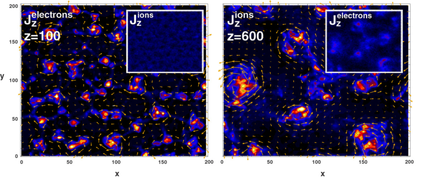
Figure 3.1: The left hand side panel shows the longitudinal electron current density through a transverse cut at $z=100$, with a small inset showing the ion current in the same plane. The right hand side panel shows the ion current at $z=600=30\delta_{i}$, with the small inset now instead showing the electron current. The arrows represent the transverse magnetic field. Both panels are from time $t=1200$ ($240\omega_{pe}^{-1}$).

Two counter-streaming – initially quasi-neutral and cold – plasma populations are simulated. At the two-stream interface (smoothed around $z=80$) a plasma ($z<80$) streaming in the positive z-direction, with a bulk Lorentz factor $\Gamma=3$, hits another plasma ($z\geq 80$) at rest in our reference frame. The latter plasma is denser than the former by a factor of 3. Experiments have been run with both initially sharp and initially smooth transitions, with essentially the same results. The long simulation time allows the shock to gradually converge towards self-consistent jump conditions. Periodic boundaries are imposed in the $x$– and $y$–directions, while the boundaries at $z=0$ and $z=800$ are open, with layers absorbing transverse electromagnetic waves. Inflow conditions at $z=0$ are fixed, with incoming particles supplied at a constant rate and with uniform speed. At $z=800$ there is free outflow of particles. The maximum experiment duration is 480 $\omega_{pe}^{-1}$ (where $\omega_{pe}$ is the electron plasma frequency), sufficient for propagating $\Gamma\approx 3$ particles 2.8 times through the box.

3.3 Results and Discussions

The extended size and duration of these experiments make it possible to follow the two-stream instability through several stages of development; first exponential growth, then non-linear saturation, followed by pattern growth and downstream advection. We identify the mechanisms responsible for these stages below.

3.3.1 Magnetic Field Generation, Pattern Growth
and Field Transport

Encountering the shock front the incoming electrons are rapidly (being lighter than the ions) deflected by field fluctuations growing as a result of the two-stream instability (Medvedev and Loeb, 1999). The initial perturbations grow non-linear as the deflected electrons collect into first caustic surfaces and then current channels (Fig. 3.1). Both streaming and rest frame electrons are deflected, by arguments of symmetry.

In accordance with Ampere’s law the current channels are surrounded by approximately cylindrical magnetic fields (illustrated by arrows in Fig. 3.1), causing mutual attraction between the current channels. The current channels thus merge in a race where larger electron channels consume smaller, neighbouring channels. In this manner, the transverse magnetic field grows in strength and scale downstream. This continues until the fields grow strong enough to deflect the much heavier ions into the magnetic voids between the electron channels. The ion channels are then subjected to the same growth mechanism as the electrons. When ion channels grow sufficiently powerful, they begin to experience Debye shielding by the electrons, which by then have been significantly heated by scattering on the growing electromagnetic field structures. The two electron populations, initially separated in $\gamma{\bf{v}}$-space, merge to a single population in approximately $20\delta_{e}$ ($z=80$–$200$) as seen in Fig. 3.6. The same trend is seen for the ions – albeit at a rate slower in proportion to $m_{i}/m_{e}$.

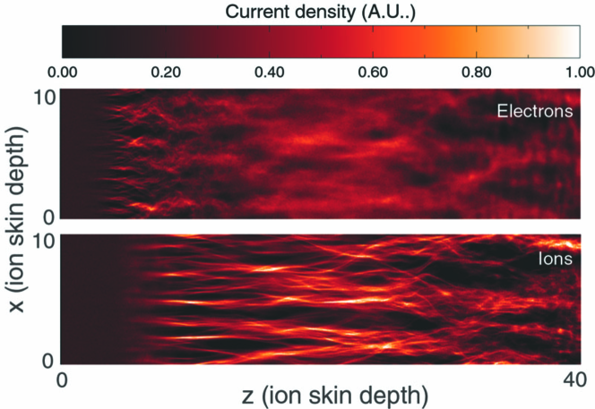
Figure 3.2: Electron (top) and ion (bottom) currents, averaged over the $y$-direction, at time $t=1200$ ($240\omega_{pe}^{-1}$). However, due to the finite propagation time of the particles, these two figures can be interpreted as earlier and later times.

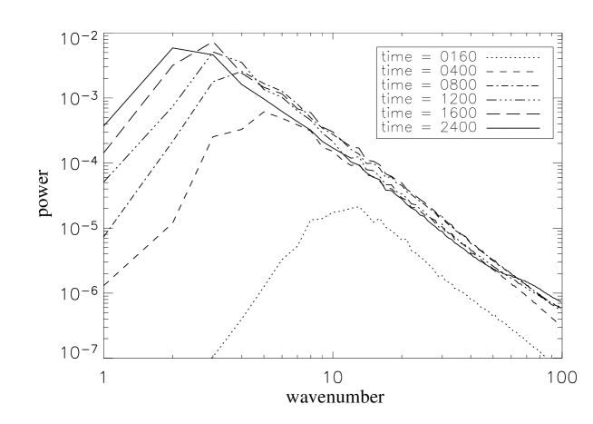
Figure 3.3: Power spectrum of ${\mathbf{B}}_{\perp}$ for $z=250$ at different times.

The Debye shielding quenches the electron channels, while at the same time supporting the ion-channels; the large random velocities of the electron population allow the concentrated ion channels to keep sustaining strong magnetic fields. Figure 3.1 shows the highly concentrated ion currents, the more diffuse – and shielding – electron currents, and the resulting magnetic field. The electron and ion channels are further illustrated in Fig. 3.2. Note the limited $z$-extent of the electron current channels, while the ion current channels extend throughout the length of the box, merging to form larger scales downstream. Because of the longitudinal current channels the magnetic field is predominantly transversal; we find $|B_{z}|/|B_{tot}|\sim 10^{-1}-10^{-2}$.

Figure 3.3 shows the temporal development of the transverse magnetic field scales around $z=250$. The power spectra follow power-laws, with the largest scales growing with time. The dominant scales at these $z$ are of the order $\delta_{i}$ at early times. Later they become comparable to $L_{x,y}$. Figure 3.4 captures this scaling behavior as a function of depth for $t=2400$ ($480\omega_{pe}^{-1}$).

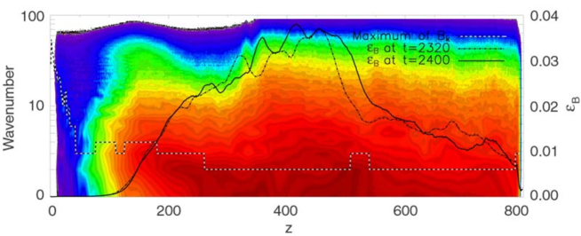
Figure 3.4: Relative electromagnetic energy density $\epsilon_{B}$. The contour color plot shows the power in the transverse magnetic field through the box distributed on spatial Fourier modes at $t=2400$ ($480\omega_{pe}^{-1}$), with the dotted line marking the wavenumber with maximum power. Superposed is the spatial distribution of $\epsilon_{B}$, averaged across the beam, at $t=2320$ ($464\omega_{pe}^{-1}$) (dashed-dotted) and $t=2400$ ($240\omega_{pe}^{-1}$)(full drawn), highlighting how EM-fields are advected down through the box.

The time evolutions of the electric and magnetic field energies are shown in Fig. 3.5. Seeded by fluctuations in the fields, mass and charge density, the two-stream instability initially grows super-linearly ($t=80-100$ = $16-20\omega_{pe}^{-1}$), reflecting approximate exponential growth in a small sub-volume. Subsequently the total magnetic energy grows more linearly, reflecting essentially the increasing volume filling factor as the non-linearly saturated magnetic field structures are advected downstream.

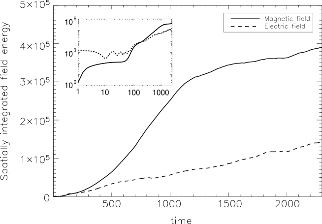
Figure 3.5: Total magnetic (full drawn) and electric (dashed) energy in the box as a function of time. The inset shows a log-log plot of the same data.

At $t\approx 1100$ the slope drops off, because of advection of the generated fields out of the box. The continued slow growth, for $t>1100$ ($220\omega_{pe}^{-1}$), reflects the increase of the pattern size with time (cf. Fig. 3.3). A larger pattern size corresponds to, on the average, a larger mean magnetic energy, since the total electric current is split up into fewer but stronger ion current channels. The magnetic energy scales with the square of the electric current, which in turn grows in inverse proportion to the number of current channels. The net effect is that the mean magnetic energy increases accordingly.

The magnetic energy density keeps growing throughout our experiment, even though the duration of the experiment (480 $\omega_{pe}^{-1}$) significantly exceeds the particle crossing time, and also exceeds the advection time of the magnetic field structures through the box. This is in contrast to the results reported by Silva et al. (2003), where the magnetic energy density decays after about 10-30 $\omega_{pe}^{-1}$. It is indeed obvious from the preceding discussion that the ion-electron asymmetry is essential for the survival of the current channels.

From the requirement that the total plasma momentum should be conserved, the (electro)magnetic field produced by the two-stream instability acquires part of the z-momentum lost by the two-stream population in the shock; this opens the possibility that magnetic field structures created in the shock migrate downstream of the shock and thus carry away some of the momentum impinging on the shock.

Our experiments show that this does indeed happen; the continuous injection of momentum transports the generated field structures downstream at an accelerated advection speed. The dragging of field structures through the dense plasma acts as to transfer momentum between the in-streaming and the shocked plasmas.

3.3.2 Thermalization and Plasma Heating

At late times the entering electrons are effectively scattered and thermalized: The magnetic field isotropizes the velocity distribution whereas the electric field generated by the $e^{-}$–$p$ charge separation acts to thermalize the populations. Figure 3.6 shows that this happens over the $\sim$ 20 electron skin depths from around $z=80$ – $200$. The ions are expected to also thermalize, given sufficient space and time. This fact leaves the massive ion bulk momentum constituting a vast energy reservoir for further electron heating and acceleration. Also seen in Fig. 3.6, the ions beams stay clearly separated in phase space, and are only slowly broadened (and heated).

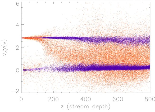
Figure 3.6: Thermalization and longitudinal acceleration, illustrated by scatter plots of the electron (orange) and ion (blue) populations. Note the back-scattered electron population ($v_{z}\gamma(v)<0$).

We do not see indications of a super-thermal tail in the heated electron distributions, and there is thus no sign of second order Fermi-acceleration in the experiment presented in this chapter. Nishikawa et al. (2003) and Silva et al. (2003) reported acceleration of particles in experiments similar to the current experiment, except for more limited sizes and durations, and the use of an $e^{-}e^{+}$ plasma (Silva et al., 2003). On closer examination of the published results it appears that there is no actual disagreement regarding the absence of accelerated particles. Whence, Nishikawa et al. (2003) refer to transversal velocities of the order of $0.2c$ (their Fig. 3b), at a time where our experiment shows similar transversal velocities (cf. Fig. 3.6) that later develop a purely thermal spectrum. Silva et al. (2003) refer to transversal velocity amplitudes up to about $0.8c$ (their Fig. 4), or $v\gamma\sim 2$, with a shape of the distribution function that appears to be compatible with thermal. In comparison, the electron distribution illustrated by the scatter plot in Fig. 3.6 covers a similar interval of $v\gamma$, with distribution functions that are close to (Lorentz-boosted) relativistic Maxwellians. Thus, there is so far no compelling evidence for non-thermal particle acceleration in experiments with no imposed external magnetic field. Thermalization is a more likely cause of the increases in transversal velocities.

Frederiksen et al. (2002) reported evidence for particle acceleration, with electron gamma up to $\sim 100$, in experiments with an external magnetic field present in the up-stream plasma. This is indeed a more promising scenario for particle acceleration experiments (although in the experiments by Nishikawa et al., 2003, results with an external magnetic field were similar to those without). Figure 3.6 shows the presence of a population of back-scattered electrons ($v_{z}\gamma<0$). In the presence of an external magnetic field in the in-streaming plasma, this possibly facilitates Fermi acceleration in the shock.

3.4 Conclusions

The experiment reported upon here illustrates a number of fundamental properties of relativistic, collisionless shocks:

1. Even in the absence of a magnetic field in the up-stream plasma, a small scale, fluctuating, and predominantly transversal magnetic field is unavoidably generated by a two-stream instability reminiscent of the Weibel-instability. In the current experiment the magnetic energy density reaches a few percent of the energy density of the in-coming beam.

2. In the case of an $e^{-}p$ plasma the electrons are rapidly thermalized, while the ions form current channels that are the sources of deeply penetrating magnetic field structures. The channels merge in the downstream direction, with a corresponding increase of the average magnetic energy with shock depth. This is expected to continue as long as a surplus of bulk relative momentum remains in the counter-streaming plasmas.

3. The generated magnetic field patterns are advected downstream at speeds intermediate between the in-coming plasma and the rest frame plasma. The electromagnetic field structures thus provide scattering centers that interact with both the fast, in-coming plasma, and with the plasma that is initially at rest. As a result the electron populations of both components quickly thermalize and form a single, Lorentz-boosted thermal electron population. The two ion populations merge much more slowly, with only gradually increasing ion temperatures.

4. The observed strong turbulence in the field structures at the shocked streaming interface provides a promising environment for particle acceleration.

We emphasize that quantification of the interdependence and development of $\epsilon_{U}$ and $\epsilon_{B}$ is accessible by means of such experiments as reported upon here.

Rather than devising abstract scalar parameters $\epsilon_{B}$ and $\epsilon_{U}$, that may be expected to depend on shock depth, media densities etc., a better approach is to compute synthetic radiation spectra directly from the models (see Chapter 7), and then apply scaling laws to predict what would be observed from corresponding, real supernova remnants and Gamma-Ray Burst afterglow shocks.

Chapter 4 Large-scale Two-Dimensional Simulations

4.1 Introduction

Large-scale simulations of collisionless electron-proton plasma shocks that are covering the full shock ramp are crucial for our interpretation of the radiation that we receive from relativistic jets (e.g. gamma-ray bursts). It is important to understand the nature and interdependencies of the shock ”parameters” $\epsilon_{e}$ and $\epsilon_{b}$. The complexity and non-linearity of collisionless shocks give PIC code simulations a central role in the process of seeking further progress in our understanding of these shocks.

Even though the continuously increasing computational power has reached a level where we may now begin to explore the full, three-dimensional collisionless shock problem, it is still only barely possible. The 3D simulations that were presented in Chapter 3 take from weeks to months to run on a modern supercomputer (parallized using 8-32 processors and 100 Gb of memory). Still it is not possible to resolve the full shock transitions region for an electron-proton collisionless plasma shock. Some of the great unanswered questions that cannot be targeted yet, because of this limitation in computer power, are for example: How large do the structures that are created by merging of current filaments grow in the non-linear phase of the Weibel two-stream instability? How many ion skin depths is the shock transition region? What is the fate of the generated magnetic structures in the downstream region where the ions are thermalized and the instability has saturated? What is the ion and electron distribution function behind the shock ramp? Does the Fermi acceleration mechanism work in collisionless shocks? Etc.

4.2 Simulations and results

To probe for answers to some of these questions, it is tempting to return to only two spatial dimensions. To test whether 2D simulations can account for the Weibel two-stream instability, we have made a 2D3V (two spatial and three velocity dimensions – sometimes referred to as $2\frac{1}{2}$D) repetition of the simulation described in Chapter 3. We use the exact same plasma densities and velocities as in the 3D experiment: In the shock rest frame, ISM particles are injected with $\Gamma=3$ into a plasma, initially at rest, with electron plasma frequency $\omega_{pe}=0.2\ c/\Delta$ (simulation units). The major difference is that the simulation box is two-dimensional with $800\times 4000$ grid zones instead of the 3D $200\times 200\times 800$. The 2D box size corresponds to $40\times 200$ ion skin depths. Compared to the 3D box, the extra grid zones in the $z$-direction is used to cover 320 grid zones upstream of the 3D box and and 2880 grid zones downstream of the 3D box.

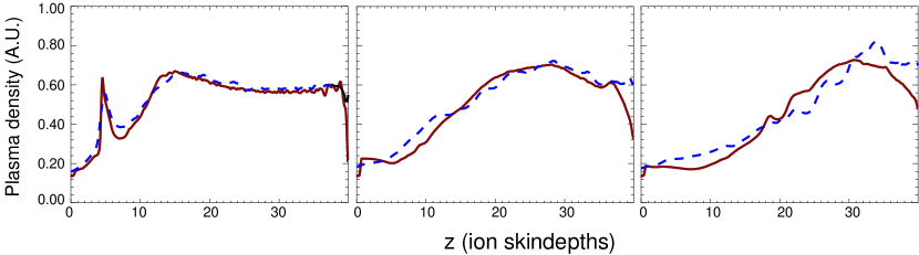
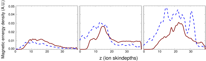
Figure 4.1: A comparison of density (top) and magnetic field generation (bottom) between 2D (dashed blue) and 3D (solid red). The three columns corresponds to snapshots taken at time $t=40$, $80$ and $120\ \omega_{pi}^{-1}$.

Figure 4.1 shows the evolution of the plasma density (top panel) and magnetic energy (bottom panel) in the 2D and 3D simulation. A good agreement between the two simulations is found, at least with respect to the evolution of the density. The minor differences are mainly caused by the artificial reflection of thermal particles at the leftmost boundary, and the drain of particles at the rightmost boundary in the 3D simulations. For the generation of magnetic field, the situation is somewhat different. In the very early stage, the field generated in the 3D simulation is stronger than in 2D, because of the extra transverse dimension that the 3D instability can collect particles from. However, at later times the growth in magnetic field in the 2D run exceeds the 3D case. This is primarily caused by two effects: 1) in the 2D box, upscattered particles (defined as shocked particles that are traveling upstream into the ISM) can generate a seed field further upstream. Such a seed field enhances the growth of the instability. This mechanism cannot be followed (yet) in the smaller 3D box. 2) ion current channels can merge to larger transverse structures. These also cannot be followed in the smaller 3D box. To a first approximation, the two-dimensional simulation shows a promising resemblance with the three-dimensional simulations, and potentially can surpass them in some respects. Encouraged by these results, we have continued the large-scale 2D simulations in order to follow the long time evolution ($t_{max}=400\omega_{pi}^{-1}$). This duration corresponds to two light crossing times of this larger box.

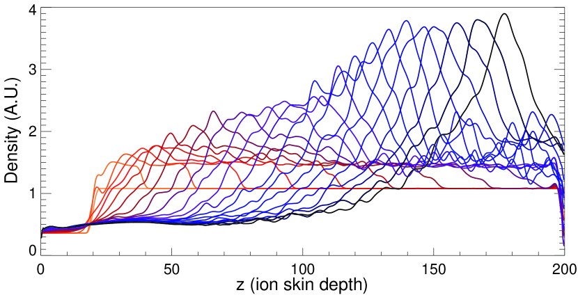
Figure 4.2: The density profile at different time, sampled in the time range $t=0-400\omega_{pi}^{-1}$ with an interval of $20\omega_{pi}^{-1}$. The different time snapshots are color coded with red for early times through blue to black at late times.

The evolution of the plasma density as function of shock depth is shown in Fig. 4.2 for different times. The time-range is $t=0-400\omega_{pi}^{-1}$ with an interval of $20\omega_{pi}^{-1}$. It is immediately clear that the initial setup is not consistent with a steady state solution. This is not surprising, since initially there are no electromagnetic fields to facilitate the momentum transfer between the injected and quiescent material. As the simulation evolves, the shock converges toward the real physical solution. In three-dimensional simulations performed by us and other groups, it has been neither temporally nor spatially possible to follow the evolution to this stage. However, the 2D simulations that we have performed cover a much larger range in space and time.

At late times, the shock reaches a steady state where the value of the main density peak is constant in time. The whole shock structure is propagating with $0.35c$ in the downstream direction. Such a steady state is expected when the computational domain covers the full shock transition ramp. In this case, the injected ISM plasma should have thermalized and merged with the shock plasma. Thus, only a single plasma population should be present in the downstream region. This is indeed the case, as seen in Fig. 4.3. The figure shows the ion (left) and electron (right) distribution functions of the momentum along the shock propagation direction ($\gamma v_{z}$), at time $t=400\omega_{pe}^{-1}$. The four different curves correspond to different regions of the computational domain ( $z=[0,50]$ , $z=[50,100]$, $z=[100,150]$, and $z=[150,200]$ ion skin depths). In the shock ramp ($z=[0,150]$ ion skin depths), where thermalization of the two ion populations (ISM and shocked) has not occurred yet, two distinct peaks are seen. In the last segment ($z=[150,200]$ ion skin depths), there exist only one single peak. This means that the ions are fully thermalized. It is also noteworthy that the merged ion population translates downstream with $\gamma v_{z}\simeq 0.4$, consistent with the estimate found from figure 4.2. Even though the peak moves relatively slowly, the particles that define the peak are moving relativistically and are continuously getting replaced with ”fresh” particles.

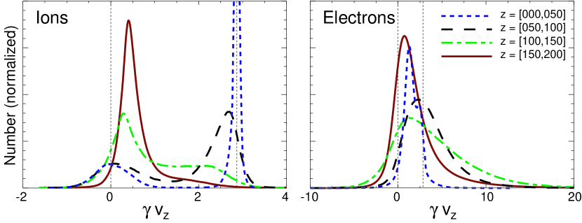
Figure 4.3: The ion (left) and electron (right) distribution functions of the momentum ($\gamma v_{z}$) along the shock propagation-direction. The particles are sampled at $t=400\omega_{pi}^{-1}$ in four different segments of the shock ramp: $z=[0,50]$ (blue, dotted), $z=[50,100]$ (black, dashed), $z=[100,150]$ (green, dot-dashed) and $z=[150,200]$ (red, solid). The (thin black dotted) vertical lines indicate $\gamma v_{z}=0$ and the injection momentum (corresponding to $\gamma=3$). Note that in the last segment ($z=[150,200]$ ion skin depths) the ions are very close to being one single population. This indicates that the full shock ramp is included in the box.

Two shock parameters of great interest are the equipartition parameters $\epsilon_{e}$ and $\epsilon_{B}$. They describe the amount of energy that is deposited in the electrons and in the magnetic field, relative to the kinetic energy of the ions. These parameters are normally treated as free parameters, available to cover our general ignorance of the details of the microphysics in collisionless shocks. Fig. 4.4 shows $\epsilon_{e}$ (left) and $\epsilon_{B}$ (right) as functions of the shock depth. It is found that the electrons reach close to equipartition with the ions. This, combined with the arguments above, allows us to conclude that the simulations cover the full shock. In the downstream region, equipartition has not yet been reached. This is because since everything moves with velocities close to the speed of light, we see earlier stages in the evolution the further downstream we look. The $\epsilon_{B}$ plot shows us that most of the field generation takes place in the foreshock. This is not surprising, since the streaming instability in its nature requires counter-streaming populations (anisotropy). Downstream, the plasma populations are fully thermalized into on single population.

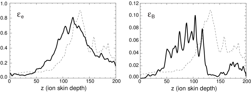
Figure 4.4: Electron (left) and magnetic (right) equipartition values ($\epsilon_{e}$ and $\epsilon_{B}$) at time $t=300\omega_{pi}^{-1}$. The dotted line in both plots shows the shape of the total plasma density for comparison. The electrons reach up to 80% of equipartition and the magnetic field up to 10%.

Finally, to give an impression of the extremely complex and non-linear nature of the collisionless shock, we present contour plots of the large-scale evolution of the shock in Figure 4.5. The figure shows the ion density structures at four different time-steps ($t=100,150,200,$ and $300\omega_{pi}^{-1}$). At early times we see that the Weibel two-stream instability is occurring semi-symmetrically at the contact discontinuities both upstream and downstream.

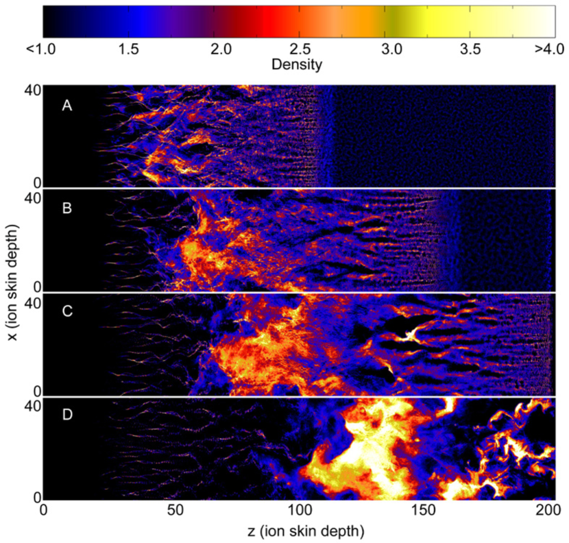
Figure 4.5: Plasma density contour plots at four different time levels A, B, C and D corresponding to $t=100,\ 150,\ 200\ \mathrm{and}\ 300\ \omega_{pi}^{-1}$

4.3 Summary

Even with the computational power available on supercomputers today, it is not possible to make three-dimensional PIC simulations that cover a full collisionless shock, while also resolving the microphysics. This has lead us to investigate whether two-dimensional simulations can include the physical processes that dominate these shocks (mainly the non-linear Weibel instability). We find that this is the case as far as 3D results exist to compare with. The density profile and generation of magnetic fields are quite similar in the two cases. Encouraged by this, we have made large-scale 2D PIC simulations of the formation of a collisionless shock, for an ejecta propagating with a bulk lorentz factor $\Gamma=3$. The simulation box covers $40\times 200$ ion skin depths (compared to the $10\times 10\times 40$ in the 3D case by Frederiksen et al. 2004, and $4\times 4\times 15$ in simulations by Nishikawa et al. 2005).

In the results we find that the 2D simulations cover a spatial region just large enough for the ISM plasma (injected into a plasma in the shock rest-frame) to thermalize and merge with the shocked plasma. Even though the initial conditions are not setup correctly, the system converges to a quasi-stationary state where at least three different regions are identified: 1) An upstream foreshock with great anisotropy, consisting of in-streaming ISM plasma and upscattered shock particles. In this region, strong magnetic field generation is taking place with $\epsilon_{B}=5-10\%$. 2) A dense, hot thermalization region where the electrons and ions are close to equipartition ($\epsilon_{e}=50-80\%$). In this region, the magnetic field is relatively weak ($\epsilon_{B}\simeq 1\%$) but still strong enough to account for most GRB afterglow estimates. 3) A hot downstream region where the magnetic field is of the order percents of equipartition. This region is clumpy, with structure sizes of the order $1-20$ ion skin depths (see Fig. 4.5).

In these 2D simulations it is found that with an initial condition where a dense plasma is at rest in the simulation frame, the resulting shock rest frame was propagating with $0.35c$ in the downstream direction. Based on these results, we plan to rerun the simulations in a frame where the dense population initially travels with $0.35c$ in the upstream direction. This would potentially allow us to follow the shock for longer periods of time.

Finally we note that the upscattering of particles might be important for Fermi acceleration. It is likely that these particles can be deflected back into the shock region. To test whether Fermi acceleration is taking place requires even larger simulations and the question can only be answered by future work.

Chapter 5 Shocks in Ambient Magnetic Fields

We now continue with an investigation of the Weibel instability in collisionless shocks in the presence of an ambient magnetic field (Hededal and Nishikawa, 2005). This scenario is important especially in the internal shock phase and in the very early afterglow, where it is possible that a magnetic field, carried from the GRB progenitor, still exist in the ejecta.

Plasma outflows from gamma-ray bursts, supernovae, and relativistic jets, in general interact with the surrounding medium through collisionless shocks. The microphysical details of such shocks are still poorly understood, which, potentially, can introduce uncertainties in the interpretation of observations. It is now well established that the Weibel two-stream instability is capable of generating strong electromagnetic fields in the transition region between the jet and the ambient plasma. However, the parameter space of collisionless shocks is vast and still remains unexplored. In this chapter, we focus on how an ambient magnetic field affects the evolution of the electron Weibel instability and the associated shock. Using a particle-in-cell code, we have performed three-dimensional numerical experiments on such shocks. We compare simulations in which a jet is injected into an unmagnetized plasma with simulations in which the jet is injected into a plasma with an ambient magnetic field both parallel and perpendicular to the jet flow. We find that there exists a threshold of the magnetic field strengths, below which the Weibel two-stream instability dominates, and we note that the interstellar medium magnetic field strength lies well below this value. In the case of a strong magnetic field parallel to the jet, the Weibel instability is quenched. In the strong perpendicular case, ambient and jet electrons are strongly accelerated because of the charge separation between deflected jet electrons and less deflected jet ions. Also, the electromagnetic topologies become highly non-linear and complex with the appearance of anti-parallel field configurations.

5.1 Introduction

The collisionless plasma condition applies to many astrophysical scenarios, including, the outflow from gamma-ray bursts (GRBs), active galactic nuclei, and relativistic jets in general. The complexity of kinetic effects and instabilities makes it difficult to understand the nature of collisionless shocks. Only recently, the increase in available computational power has made it possible to investigate the full three-dimensional dynamics of collisionless shocks.

In the context of GRB afterglows, observations indicate that shock-compressed magnetic field from the interstellar medium (ISM) is several orders of magnitude too weak to match observations. Particle-in-cell (PIC) simulations have revealed that the Weibel two-stream instability is capable of generating the required electromagnetic field strength of the order of percents of equipartition value (Kazimura et al., 1998; Medvedev and Loeb, 1999; Nishikawa et al., 2003, 2005; Silva et al., 2003; Frederiksen et al., 2004). Furthermore, PIC simulations have shown that in situ non thermal particle acceleration takes place in the shock transition region (Hoshino and Shimada, 2002; Hededal et al., 2004; Saito and Sakai, 2003). Three-dimensional simulations using $\sim 10^{7}$ electron-positron pairs by Sakai and Matsuo (2004) showed how complex magnetic topologies are formed when injecting a mildly relativistic jet into a force-free magnetic field with both parallel and perpendicular components. With a two-dimensional analysis, Saito and Sakai (2003) found that an ambient parallel magnetic field can quench the two-stream instability in the weakly relativistic case. In this chapter, we use three-dimensional PIC experiments to investigate how the two-stream instability is affected by the presence of an ambient magnetic field. Using up to $\sim 10^{9}$ particles and $125\times 125\times 1200$ grid zones, we investigate the development of complex magnetic topologies when injecting a fully relativistic jet (bulk Lorentz factor $\Gamma=5$) into an ambient magnetized plasma. Using varying field strengths, we focus on the case of a transverse magnetic field and compare it with the case of a parallel magnetic field. The simulations are mainly concerned with the electron dynamics since processes involving the heavier ions evolve on much longer timescales.

5.2 The numerical experiments

We use the PIC code described by Frederiksen et al. (2004). The code works from first principles and evolves the equation of motion for the particles together with Maxwell’s equations. In the simulation experiments, we inject an electron-proton plasma (a jet) into an ambient plasma (the ISM) initially at rest (Fig. 5.1). The jet is moving with a relativistic velocity of $0.98c$ along the $z$-direction, corresponding to Lorentz factor $\gamma_{jet}=5$. The ion-to-electron mass ratio is set to $m_{\rm i}/m_{\rm e}=20$. The jet plasma and the ambient plasma have the same density, $n$, and the corresponding electron plasma rest-frame frequency $\omega_{pe}\equiv[ne^{2}/(m_{e}\epsilon_{0})]=0.035\Delta_{t}^{-1}$ ($e$ is the unit charge, $\epsilon_{0}$ the vacuum permittivity, and $\Delta_{t}$ the simulation time unit). We choose this low value in order to properly resolve the microphysics. Initially, the interface between the ambient and the injected plasma is located at $z=3\lambda_{e}$, where $\lambda_{e}$ is the electron skin depth defined as $\lambda_{e}\equiv c/\omega_{pe}=28.6\Delta_{x}$ ($c$ is the speed of light, and $\Delta_{x}$ the grid size). The time step and grid size obey the Courant-Friedrichs-Levy condition $\Delta_{t}=0.5\Delta_{x}/c$. Both plasma populations are, in their respective rest frames, Maxwellian distributed with a thermal electron velocity $v_{th}\simeq 0.03c$. This temperature allows us to numerically resolve the plasma Debye length with at least one grid length.

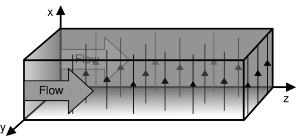
Figure 5.1: Schematic example of the simulation setup. Jet plasma is homogeneously and continuously injected in the $z$-direction throughout the $x-y$ plane at $z=0$. Inside, the box is populated by a plasma population, initially at rest. In this specific example, an ambient magnetic field is set up in the $x$-direction (perpendicular case).

We consider three different ambient magnetic configurations: no magnetic field, a magnetic field parallel to the flow, and a magnetic field perpendicular to the flow. The magnetic field is initially setup to be homogeneous and at rest in the ambient plasma. The experiments are carried out with 1 billion particles inside $125\times 125\times 1200$ grid zones. In terms of electron skin depths, this corresponds to $4.4\times 4.4\times 42\lambda_{e}$. The boundary conditions are periodic in the direction transverse to the jet flow ($x,y$). In the parallel direction, jet particles are continuously injected at the leftmost boundary ($z=0$). At the leftmost and rightmost $z$ boundary, electromagnetic waves are absorbed, and we allow particles to escape in order to avoid unphysical feedback. The total energy throughout the simulations is conserved with an error less than $1\%$.

5.3 Results

Initially, we ran simulations with no ambient magnetic field and observed the growth of the Weibel two-stream instability also found in previous work (Kazimura et al., 1998; Medvedev and Loeb, 1999; Nishikawa et al., 2003, 2005; Silva et al., 2003; Frederiksen et al., 2004). The Weibel two-stream instability works when magnetic perturbations transverse to the flow collect streaming particles into current bundles that in turn amplify the magnetic perturbations. In the non-linear stage, we observe how current filaments merge into increasingly larger patterns. The electromagnetic energy grows to $\epsilon_{B}\simeq 1\%$, where $\epsilon_{B}$ describes the amount of total injected kinetic energy that is converted to magnetic energy.

5.3.1 Parallel Magnetic Field

In the presence of a strong magnetic field component parallel to the flow, particles are not able to collect into bundles, since transverse velocity components are deflected. We have performed five runs, with parallel magnetic fields corresponding, respectively, to $\omega_{pe}/\omega_{ce}=$40, 20, 10, 5, and 1, while keeping $\omega_{pe}$ constant; $\omega_{ce}=eB/(\gamma_{jet}m_{e})$ is the jet electron gyrofrequency. The resulting field generation efficiency can be seen in Fig. 5.2 at $t=21\omega_{pe}^{-1}$ where the jet front has reached $z=23\lambda_{e}$. In the case of $\omega_{pe}/\omega_{ce}=40$, the Weibel instability overcomes the parallel field, and although initially slightly suppressed, it eventually evolves as in the case of no ambient magnetic field. Increasing the magnetic field to $\omega_{pe}/\omega_{ce}=1$ effectively suppresses the instability. Thus, for an ISM strength magnetic field ($\omega_{pe}/\omega_{ce}\simeq 1500$) parallel to the plasma flow, the Weibel two-stream instability evolves unhindered, and the generated field will exceed the ISM field. We find from the simulations that it would take a milligauss strength parallel magnetic field to effectively quench the instability for a $\gamma=5$ jet expanding in an environment with density similar to the ISM.

Figure 5.2: Growth of the Weibel two-stream instability for different strengths of the parallel ambient magnetic field at time $t=21\omega_{pe}^{-1}$. Here we show the effectiveness of the field generation, as measured by the average transverse magnetic field amplitude as a function of $z$. The solid line corresponds to $\omega_{pe}/\omega_{ce}=40$, the dotted line to 20, the dashed line to 10, the dot-dashed line to 5, and the triple-dot-dashed line to 1. The case of no ambient magnetic field is very similar to that of $\omega_{pe}/\omega_{ce}=40$. The magnetic field amplitude is in arbitrary units

The left panel of Fig. 5.3 shows the resulting electron momentum distribution function for different values of $\omega_{pe}/\omega_{ce}$ at $t=30\omega_{pe}^{-1}$. Since the presence of a strong parallel magnetic field suppresses the generation of a transverse magnetic field, there exists no mechanism that can heat the electrons and transfer momentum between the two electron populations. Thus the jet plasma propagates unperturbed. Where there is no parallel magnetic field or only a weak magnetic field ($\omega_{pe}/\omega_{ce}=1500$), we observe how the jet and ambient plasma is heated and how momentum is transferred between the two populations.

Figure 5.3: Normalized electron momentum distribution functions at time $30\omega_{pe}^{-1}$. The left panel is for runs with an ambient magnetic field parallel to the injected plasma with $\omega_{pe}/\omega_{ce}=$ 1 (solid line), 20 (dotted line), 40 (dashed line), and 1500 (dot-dashed line). The right panel is for runs in which the initial magnetic field is perpendicular to the inflow and $\omega_{pe}/\omega_{ce}=$ 5 (solid line), 20 (dotted line), 40 (dashed line) and 1500 (dot-dashed line). The vertical line shows the injected momentum $\gamma=5$. The distribution functions are for electrons with $z>15\lambda_{e}$.

5.3.2 Perpendicular Magnetic Field

We have performed experiments with an ambient magnetic field perpendicular to the jet flow (Fig. 5.1), with field strengths corresponding to $\omega_{pe}/\omega_{ce}$=1500, 40, 20 and 5. By including the displacement current, one can derive the relativistic Alfvén speed $v_{A}^{-2}=c^{-2}+(v_{A}^{non-rel.})^{-2}\simeq c/[1+(\omega_{pe}/\omega_{ce})^{2}(m_{i}/m_{e})\gamma_{jet}^{-2}]^{1/2}$, where $v_{A}^{non-rel.}=B/[\mu_{0}n(m_{i}+m_{e})]^{1/2}$ is the non-relativistic counterpart. From this we calculate the corresponding relativistic Alfv́en Mach numbers $\gamma_{jet}v_{jet}/v_{A}=$ 6572, 175, 88, and 22.

Again, the $\omega_{pe}/\omega_{ce}=1500$ run has been chosen because it resembles the typical density and microgauss magnetic field strength of the ISM. We find that the magnetic field generated by the two-stream instability dominates the ambient magnetic field, and the result resembles the case with no ambient magnetic field. Furthermore, as expected in both the parallel and perpendicular cases, the electron momentum distributions (Fig. 5.3) are very similar, except for a weak merging between the ambient and jet electrons in the perpendicular case.

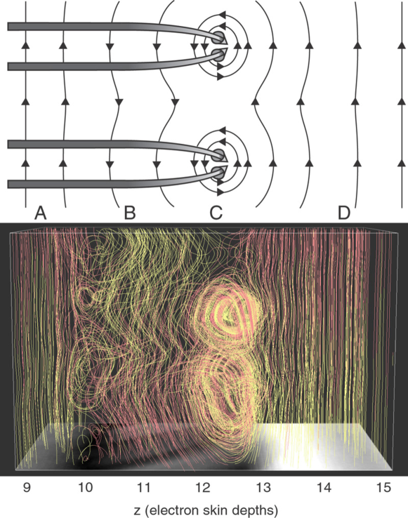
Figure 5.4: Snapshot at $t=16\omega_{pe}^{-1}$ of the highly complicated magnetic field topology resulting when a jet is injected into a plasma with an ambient magnetic field transverse to the jet flow. The bottom panel shows magnetic field lines in a subsection of the computational box (from $z=9\lambda_{e}$ to $z=15\lambda_{e}$. The top panel refers to a schematic explanation in the $x-z$ plane: Jet electrons are bent by the ambient magnetic field (region A). As a result of the Weibel instability, the electrons bundle into current beams (region C) that in turn reverse the field topology (region B). This will eventually bend the jet beam in the opposite direction.

In the run with $\omega_{pe}/\omega_{ce}=20$, the result differs substantially from the previous cases. With reference to Fig. 5.4, we describe the different stages of the evolution: Initially, the injected particles are deflected by the ambient magnetic field. The magnetic field is piled up behind the jet front, and the enhanced magnetic fields bend jet electron trajectories sharply. This has two implications. First, the ions, being more massive, penetrate deeper than the deflected electrons. This creates a charge separation near the jet head that effectively accelerates both ambient and injected electrons behind the ion jet front as shown in Fig. 5.5. Second, the deflected electrons eventually become subject to the Weibel two-stream instability. This forms electron current channels at some angle to the initial direction of injection, as shown in the upper panel of Fig. 5.4. Around these current channels, magnetic loops are induced (Fig. 5.4, region C). Magnetic islands are formed and the ambient magnetic field is reversed behind the loops (region B). In this region, we find acceleration of electrons in the $x$-direction. The activity in this region has similarities to reconnection, but it is beyond the scope of this thesis to investigate this topic.

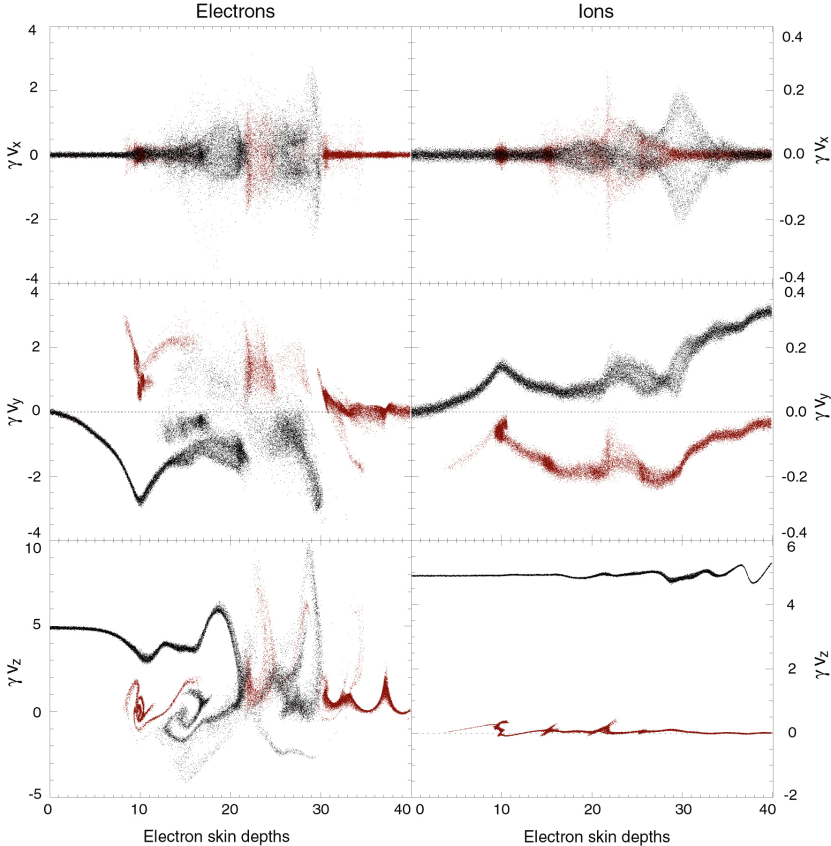
Figure 5.5: Phase-space plot of electrons (left column) and ions (right column) at time $t=30\omega_{pe}^{-1}$. The data is from a simulation of a shock with transverse ambient magnetic field corresponding to $\omega_{pe}/\omega_{ce}=20$. The three rows correspond to $\gamma v_{x}$, $\gamma v_{y}$ and $\gamma v_{z}$. The jet plasma (black dots) are injected at $z=0$ with $\gamma=5$. The ambient electrons (red dots) are initially at rest but are strongly accelerated by the jet.

In other regions, the ambient magnetic field is strongly compressed, and this amplifies the field strength up to 5 times the initial value. As a result, parts of the jet electrons are reversed in their direction. This may be seen from Fig. 5.5, which shows a phase-space plot of both ambient and jet electrons at $t=30\omega_{pe}^{-1}$. We see several interesting features here. In the region $z=(15-21)\lambda_{e}$, we observe how ambient electrons are swept up by the jet. Behind the jet front, both ambient and jet electrons are strongly accelerated since the jet ions, being heavier, take a straighter path than the jet electrons, and this creates a strong charge separation. The excess of positive charge at the very front of the jet head is very persistent and hard to shield since the jet ions are moving close to the speed of light. Thus, there is a continuous transfer of $z$-momentum from the jet ions to the electrons. In the case of the perpendicular ambient field, more violent processes take place than in the case of the parallel field, which may be seen in Fig. 5.3 (right panel). Here we see that mixing of the two plasma populations is much more effective for the perpendicular case. However, the spectrum of the electron’s momentum is highly nonthermal, with strong acceleration of both jet and ambient electrons. The cutoff in electron acceleration depends on the magnetic field strength. The maximum ($\gamma v_{\parallel}\approx 10$) at $z=20\lambda_{e}$ in Fig 5.5 corresponds to the cutoff shown by the dotted line in the right panel in Fig. 5.3. It should be noted that the current channels that are caused by the bent jet electron trajectories at the early time, as shown in Fig. 5.4, are also seen in Fig. 5.5. The first current channels have moved to around $z=20\lambda_{e}$. At $z=15\lambda_{e}$, a second current channel is created by the deflected jet electrons. This periodic phenomenon involves the ions (Fig. 5.6) in a highly nonlinear process but is beyond the scope of this thesis and will be investigated in subsequent work.

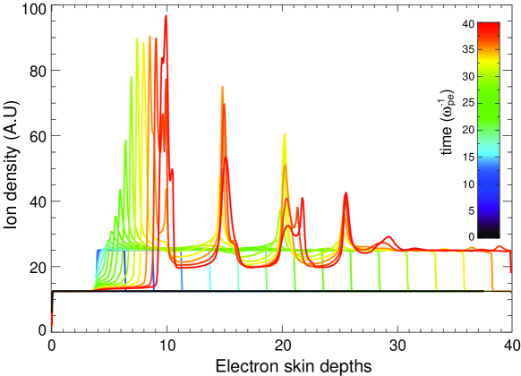
Figure 5.6: The ion density averaged over the box width as a function of shock depth. The different colors correspond to different times. The simulation is for $\omega_{pe}/\omega_{ce}=20$. The distance between each peak is comparable to the ion skin depth.

5.4 Conclusions

Using a three-dimensional relativistic particle-in-cell code, we have investigated how an ambient magnetic field affects the dynamics of a relativistic jet in the collisionless shock region. We have examined how the different ambient magnetic topology and strength affect the growth of the electron Weibel two-stream instability and the associated electron acceleration. This instability is an important mechanism in collisionless shocks. It facilitates momentum transfer between colliding plasma populations (Kazimura et al., 1998; Medvedev and Loeb, 1999; Nishikawa et al., 2003, 2005; Silva et al., 2003; Frederiksen et al., 2004) and can accelerate electrons to nonthermal distributions (Hoshino and Shimada, 2002; Hededal et al., 2004; Saito and Sakai, 2003). Collisionless shocks are found in the interface between relativistic outflows (e.g., from gamma-ray bursts and active galactic nuclei) and the surrounding medium (e.g., the ISM).

We find substantial differences between the cases of ambient magnetic fields transverse and parallel to the jet flow. However, common to both cases is that it takes an ambient magnetic field strength much stronger than the strength of the magnetic field typically found in the ISM to effectively suppress the Weibel two-stream instability. In the case of a parallel magnetic field, $\omega_{pe}/\omega_{ce}$ must be smaller than 5 to effectively suppress the instability. This result is in good agreement with two-dimensional simulations by Saito and Sakai (2003), and thus this limit seems independent of $\gamma_{jet}$. For a typical ISM density of $10^{6}\mathrm{m}^{-3}$, this corresponds to a milligauss magnetic field. We emphasize the role of $\omega_{pe}/\omega_{ce}$ as an important parameter for collisionless shocks, as was also pointed out by Shimada and Hoshino (2004).

In the case of perpendicular injection, the dynamics are different from the parallel injection. Here, the electrons are deflected by the magnetic field, and this creates a charge separation from the less deflected ions. The charge separation drags the ambient and jet electrons, and consequently they are strongly accelerated along the $z$-direction. Furthermore, as a result of the Weibel instability, current channels are generated around the ambient magnetic field, which is curled and locally reversed.

These simulations provide insights into the complex dynamics of relativistic jets. Further investigations are required to understand the detailed physics involved. Larger simulations (above $10^{9}$ particles) with longer boxes are needed to cover the instability domain of the ions, to investigate the full evolution of the complicated dynamics, and to resolve the whole shock ramp.

Chapter 6 Non–Fermi Acceleration in Plasma Shocks

Collisionless plasma shock theory, which applies, for example, to the afterglow of gamma-ray bursts, still contains key issues that are poorly understood. In this chapter, I discuss the results of charged particle dynamics in a highly relativistic collisionless shock numerically using $\sim 10^{9}$ particles (Hededal et al., 2004). We find a power-law distribution of accelerated electrons, which upon detailed investigation turns out to originate from an acceleration mechanism that is decidedly different from Fermi acceleration. Electrons are accelerated by strong filamentation instabilities in the shocked interpenetrating plasmas and coincide spatially with the power-law–distributed current filamentary structures. These structures are an inevitable consequence of the now well-established Weibel–like two–stream instability that operates in relativistic collisionless shocks. The electrons are accelerated and decelerated instantaneously and locally: a scenery that differs qualitatively from recursive acceleration mechanisms such as Fermi acceleration. The slopes of the electron distribution power-laws are in concordance with the particle power law spectra inferred from observed afterglow synchrotron radiation in gamma-ray bursts, and the mechanism can possibly explain more generally the origin of nonthermal radiation from shocked interstellar and circumstellar regions and from relativistic jets.

6.1 Introduction

Given the highly relativistic conditions in the outflow from gamma-ray bursts (GRBs), the mean free path for particle Coulomb collisions in the afterglow shock is several orders of magnitude larger than the fireball itself. In explaining the microphysical processes that work to define the shock, MHD becomes inadequate and collisionless plasma shock theory stands imperative. In particular, two key issues remain, namely, the origin and nature of the magnetic field in the shocked region and the mechanism by which electrons are accelerated from a thermal population to a power-law distribution $N(\gamma)d\gamma\propto\gamma^{-p}$. Both ingredients are needed to explain the observed afterglow spectra (e.g. Kumar, 2000; Panaitescu and Kumar, 2001).

Regarding the origin of the magnetic field in the shocked region, observations are not compatible with a compressed interstellar magnetic field, which would be orders of magnitude smaller than needed (Gruzinov and Waxman, 1999). It has been suggested that a Weibel–like two–stream instability can generate a magnetic field in the shocked region (Medvedev and Loeb 1999; Frederiksen et al. 2002; Nishikawa et al. 2003; Silva et al. 2003). Computer experiments by Frederiksen et al. (2004) showed that the nonlinear stage of a two–stream instability induces a magnetic field in situ with an energy content of a few percent of the equipartition value, consistent with that required by observations.

Fermi acceleration (Fermi, 1949) has, so far, been widely accepted as the mechanism that provides the inferred electron acceleration. It has been employed extensively in Monte Carlo simulations (e.g. Niemiec and Ostrowski (2004) and references therein), where it operates in conjunction with certain assumptions about the scattering of particles and the structure of the magnetic field. The mechanism has, however, not been conclusively demonstrated to occur in ab initio particle simulations. As pointed out by Niemiec and Ostrowski (2004), further significant advance in the study of relativistic shock particle acceleration is unlikely without understanding the detailed microphysics of collisionless shocks. Also, recently Baring and Braby (2004) found that particle distribution functions (PDFs) inferred from GRB observations are in contradistinction with standard acceleration mechanisms such as diffusive Fermi acceleration.

In this chapter, we study ab initio the particle dynamics in a collisionless shock with bulk Lorentz factor $\Gamma=15$. We find a new particle acceleration mechanism, which we present in Section 6.2. Detailed numerical results are presented and interpreted in Section 6.3, while Section 6.4 contains the conclusions.

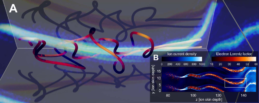
Figure 6.1: (A) Ray-traced electron paths (red) and current density (blue). The colors of the electron paths reflect their four-velocity according to the color table in the inset (B). The shadows are equivalent to the $x$ and $y$ projections of their paths. The ion current density is shown with blue colors according to the color table in the inset. The inset also shows the ion current density (blue) integrated along the $x$-axis with the spatial distribution of fast-moving electrons (red) over plotted. The main figure is an enlargement of the white square in the inset.

6.2 A new acceleration mechanism

We have performed a series of numerical experiments where collisionless shocks are created by two colliding plasma populations. These experiments are described in more detail below, but a common feature is that the electron PDF has a high-energy tail that is power-law distributed. By carefully examining the paths of representative accelerated electrons, tracing them backward and forward in time, we have been able to identify the mechanism responsible for their acceleration. The acceleration mechanism, which as far as we can tell has not been discussed in the literature previously, works as follows:

When two nonmagnetized collisionless plasma populations interpenetrate, current channels are formed through a Weibel–like two–stream instability (Medvedev and Loeb 1999; Frederiksen et al. 2002; Nishikawa et al. 2003; Silva et al. 2003). In the nonlinear stage of evolution of this instability, ion current channels merge into increasingly stronger patterns, while electrons act to Debye shield these channels, as shown by Frederiksen et al. (2004). That work further showed that a Fourier decomposition of the transverse ion current filaments exhibits power-law behavior, which has been recently confirmed by Medvedev et al. (2005).

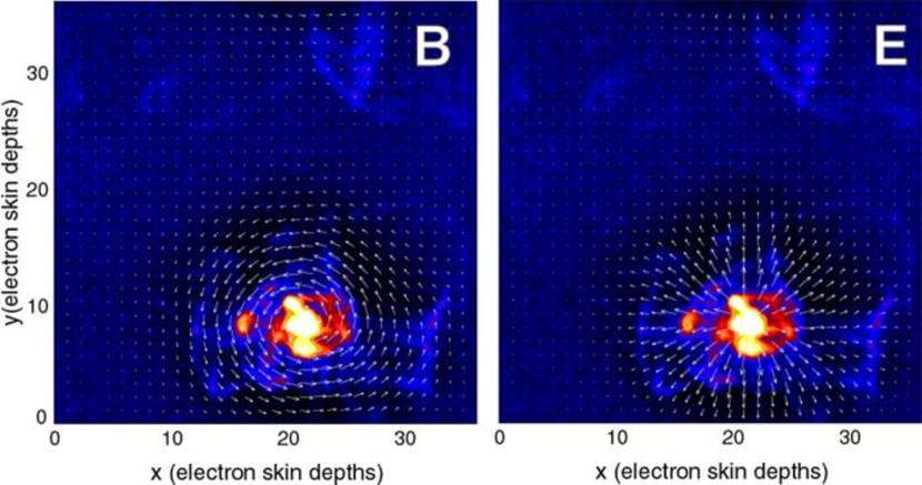
Figure 6.2: A contour plot of the ion current strength with arrows overplotted to represent the magnetic field (left panel) and the electric field (right panel).

Figure 6.2 presents the electric and magnetic field in the vicinity of an ion current channel, generated by the Weibel two-stream instability. At distances less than the Debye length, the ion current channels are surrounded by transverse electric fields that accelerate the electrons toward the current channels. However, the magnetic fields that are induced around the current channels act to deflect the path of the accelerated electrons, boosting them instead in the direction of the ion flow. Since the forces working are caused by quasi–stationary fields, the acceleration is a simple consequence of potential energy being converted into kinetic energy. Therefore, the electrons are decelerated again when leaving the current channel and reach their maximal velocities at the centers of the current channels. Hence, as illustrated by Fig. 6.1B, the spatial distribution of the high-energy electrons is a direct match to the ion current channels and the properties of the accelerated electrons depend primarily on the local conditions in the plasma.

One might argue that the near–potential behavior of the electrons, where they essentially must lose most of their energy to escape from the current channels, would make the mechanism uninteresting as an acceleration mechanism since fast electrons cannot easily escape. However, this feature may instead be a major advantage, since it means that energy losses due to escape are small and that the electrons remain trapped long enough to have time to lose their energy via a combination of bremsstrahlung and synchrotron or jitter radiation. We observe that only a very small fraction of the electrons manage to escape, while still retaining most of their kinetic energy. This happens mainly at sudden bends or mergers of the ion channels, where the electron orbits cannot be described in terms of a particle moving in a static electromagnetic field.

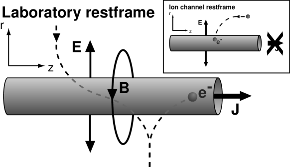
Figure 6.3: Ion current channel surrounded by an electric and a magnetic field. A schematic drawing of the scenario in Fig. 6.2, seen from the side. Electrons in the vicinity of the current channels are thus subject to a Lorentz force with both an electric and magnetic component, working together to accelerate the electrons along the ion flow. Crossing the center of the channel, the process reverses, leading to an oscillating movement along the channel.

To analyze the acceleration scenario quantitatively, we use the sketch in Fig. 6.3. We assume that the ion current channel has radius $R$, that the total charge inside the cylinder per unit length is $\rho_{c}$, and that the ions stream with velocity $u$ in the laboratory rest frame (see Fig. 6.3 and inset for definition of rest frames). Consider an electron with charge $-q$ and mass $m$ at a distance $r$ from the center of the channel, initially having no velocity components perpendicular to the cylinder. If we analyze everything in the ion channel rest frame, the problem reduces to electrostatics and it is possible to analytically calculate the change in four-velocity of the electron when it reaches the surface of the cylinder. Since the electric force only works along the $r$-axis, the four-velocity along the $z$–axis of the electron is conserved in the ion channel rest frame. Hence, we can calculate both the total change in energy and the change in the different velocity components. Returning to the laboratory rest frame, we find

$$\Delta\gamma_{electron} =\frac{q\rho_{c}}{2\pi mc^{2}\epsilon_{0}}\ln\frac{r}{R}$$ (6.1)

$$\Delta(\gamma v_{z})_{electron} =u\Delta\gamma_{electron}\,.$$ (6.2)

The change in the Lorentz boost is directly proportional to the total charge inside the channel and inversely proportional to the electron mass. Debye shielding reduces the electric field further away from the ion channel, so the estimate above is only valid for distances smaller than a Debye length.

6.3 Computer Experiments

The experiments were performed with the three-dimensional relativistic kinetic and electromagnetic particle–in–cell code described by Frederiksen et al. (2004). The code works from first principles, by solving Maxwell’s equations for the electromagnetic fields and solving the Lorentz force equation of motion for the particles.

Two colliding plasma populations are set up in the rest frame of one of the populations (downstream, e.g., a jet). A less dense population (upstream, e.g. the interstellar medium) is continuously injected at the left boundary with a relativistic velocity corresponding to a Lorentz factor $\Gamma=15$. The two populations initially differ in density by a factor of 3. We use a computational box with $125\times 125\times 2000$ grid points and a total of $8\times 10^{8}$ particles. The ion rest-frame plasma frequency in the downstream medium is $\omega_{pi}=0.075$, rendering the box 150 ion skin depths long. The electron rest-frame plasma frequency is $\omega_{pe}=0.3$ in order to resolve also the microphysics of the electrons. Hence, the ion-to-electron mass ratio is $m_{i}/m_{e}=16$. Other mass ratios and plasma frequencies were used in complementary experiments. Initially, both plasma populations are unmagnetized.

The maximum experiment duration has $t_{max}=$ 340 $\omega_{pi}^{-1}$, which is sufficient for the continuously injected upstream plasma ($\Gamma=15$, $v\sim c$) to travel 2.3 times the length of the box. The extended size and duration of these experiments enable observations of the streaming instabilities and concurrent particle acceleration through several stages of development (Frederiksen et al., 2004). Momentum losses to radiation (cooling) are presently not included in the model. We have, however, verified that none of the accelerated particles in the experiment would be subject to significant synchrotron cooling. The emitted radiation may thus be expected to accurately reflect the distribution of accelerated electrons.

When comparing numerical data with eq. 6.1, we take $r$ to be the radius where Debye shielding starts to be important. Using a cross section approximately in the middle of Fig. 6.1, we find $\Delta(\gamma v_{z})_{electron}=58\ln(r/R)$. It is hard to determine exactly when Debye shielding becomes effective, but looking at electron paths and the profile of the electric field, we estimate that $\ln(r/R)\approx 1.3$. Consequently, according to eq. 6.1, the maximally attainable four-velocity in this experiment is in the neighbourhood of $(\gamma v_{z})_{max}=75$. This is in good agreement with the results from our experiments, where the maximum four-velocity is $(\gamma v_{z})_{max}\simeq 80$.

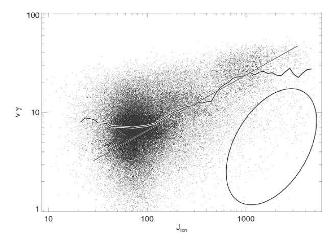
Figure 6.4: A scatter plot of the local ion current density $J_{Ion}$ versus the four velocity of the electrons in a region downstream of the shock. Overplotted is a line (thin) showing the average four velocity as a function of $J_{Ion}$, and a line (thick) showing a straight line fit. Because ’cold’ trapped thermal electrons (indicated with the ellipse) exist inside the ion current channel they count towards lowering the average four velocity at high $J_{Ion}$. If we cleaned our scatter plot, statistically removing all thermal electrons we would see a much tighter relation. Such cleaning, though, is rather delicate and could introduce biases by itself. The trend is clearly there though even for the ’raw’ data.

The theoretical model does of course not cover all details of the experiment. For example, in general the electrons also have velocity components parallel to the magnetic field; instead of making one-dimensional harmonic oscillations in the plane perpendicular to the current channel, the electrons will describe ellipsoidal paths. Fig. 6.1 shows the path of two electrons in the vicinity of an ion channel. But, overall, the electrons behave as expected from the model considerations. Consequently, high-speed electrons are tightly coupled to the ion channels, as clearly illustrated by Fig. 6.1B.

Figure 6.5 shows that the electrons are power-law–distributed at high energies, with index $p=2.7$. The electrons at the high gamma cutoff are found where the ion current peaks, as may be seen from Fig. 6.4. The maximum ion current is limited by the size of our box; larger values would probably be found if the merging of current channels could be followed further downstream. The PDF is not isotropic in any frame of reference because of the high anisotropy of the Weibel-generated electromagnetic field. The power-law in the electron PDF is dominant for $10<\gamma<30$. Likewise, a power law dominates the ion current channel strength, $J_{Ion}$, for $100<J_{Ion}<1000$ (inset). A relation between the power-law distributions of these two quantities on their respective intervals is provided with Fig. 6.4: we see that the average four-velocity is proportional (straight line fit) to a power of the local ion current density on their respective relevant intervals, $10<\gamma<30$ and $100<J_{Ion}<1000$. Their kinship stems from the fact that acceleration is local. The value $J_{Ion}$ has a power-law tail, and its potential drives the high energy distribution of the electrons according to eq. 6.1, thus forming a power-law–distributed electron PDF.

Measuring the rate at which the in–streaming ions transfer momentum to the ion population initially at rest allows us to make a crude estimate of the length scales over which the two–stream instability in the current experiment would saturate owing to ion thermalization. A reasonable estimate appears to be approximately 10 times the length of the current computational box, or about 1500 ion skin depths. Assuming that the shock propagates in an interstellar environment with a plasma density of $\sim 10^{6}$ m^-3, we may calculate a typical ion skin depth. Comparing this value with the upstream ion skin depth from our experiments, we find that the computational box corresponds to a scale of the order of $10^{7}$ m, or equivalently that the collisionless shock transition region of the current experiment corresponds to about $10^{8}$ m. For an ion with a Lorentz factor $\gamma=15$, this length corresponds roughly to 40 ion gyro radii in the average strength of the generated magnetic field. But we stress that the in–streaming ions do not really gyrate, since they mainly travel inside the ion current channels where the magnetic field, by symmetry, is close to zero. Also, the strong electromagnetic fields generated by the Weibel instability and the nonthermal electron acceleration, which is crucial from the interpretation of GRB afterglow observations, emphasize the shortcoming of MHD in the context of collisionless shocks.

By rescaling the experiment to physical units we find that the electrons are accelerated to maximum energies in the neighbourhood of 5 GeV. Even further acceleration may occur as ion channels keep growing down stream, outside of our computational box.

The scaling estimates above depend, among other things, on plasma densities, the bulk Lorentz factor, and the mass ratio ($m_{i}/m_{e}$). A parameter study is necessary to explore these dependencies, but this is beyond the scope of this thesis. We thus stress that the extrapolations performed here are speculative and that unresolved physics could influence the late stages of the instability in new and interesting ways.

When the in–streaming ions are fully thermalized, they can no longer support the magnetic field structures. Thus, one might speculate that the radiating region of the GRB afterglow is very thin, as suggested by Rossi and Rees (2003). Furthermore, traditional synchrotron radiation theory does not apply to an intermittent magnetic field generated by the two–stream instability, since the electron gyroradii often are larger than the scales of the magnetic field structures. We emphasize the importance of the theory of jitter radiation (Medvedev, 2000).

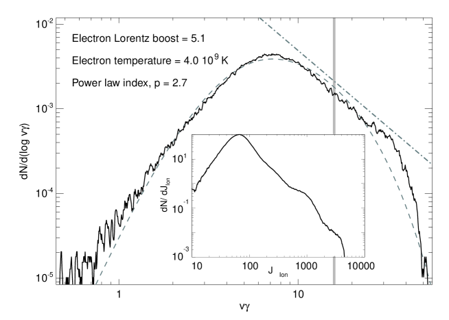
Figure 6.5: The normalized electron particle distribution function downstream of the shock. The dot–dashed line is a power law fit to the non–thermal high energy tail, while the dashed curve is a Lorentz-boosted thermal electron population. The histogram is made from the four velocities of electrons in a thin slice in the $z$–direction of the computational box. The grey vertical line at $\gamma v=15$ indicates the injection momentum. The inset shows a similar histogram for ion current density sampled in each grid point in the same slice. The bump in the inset is a statistical fluctuation caused by a single ion channel.

6.4 Conclusions

We have proposed a new acceleration mechanism for electrons in collisionless shocks. The theoretical considerations were suggested by particle–in–cell computer experiments, which also allowed quantitative comparisons with the theoretical predictions. We have shown that the nonthermal acceleration of electrons is directly related to the ion current channels in the shock transition zone. The results are applicable to interactions between relativistic outflows and the interstellar medium. Such relativistic outflows occur in GRB afterglows and in jets from compact objects (Fender et al., 2004). The suggested acceleration scenario might overcome some of the problems pointed out by Baring and Braby (2004) regarding the apparent contradiction between standard Fermi acceleration and spectral observations of GRBs.

The mechanism has important implications for the way we understand and interpret observations of collisionless shocks:

• The acceleration mechanism is capable of creating a power-law electron distribution in a collisionless shocked region. In the computer experiment presented here, a bulk flow with $\Gamma=15$ results in a power-law slope $p=2.7$ for the electron PDF. Additional experiments are needed to disentangle which parameters determine the exact value of the slope.

• The acceleration is local; electrons are accelerated to a power law in situ. Therefore, the observed radiation field may be tied directly to the local conditions of the plasma and could be a strong handle on the physical processes.

• Our results strengthen the point already made by Frederiksen et al. (2004) that the fractions of the bulk kinetic energy that go into in the electrons and the magnetic field, $\epsilon_{e}$ and $\epsilon_{B}$, respectively, are not free and independent parameters of collisionless shock theory. Most likely, they represent interconnected parts of the same process.

• In the case of a weak or no upstream magnetic field, the Weibel–like two–stream instability is able to provide the necessary electromagnetic fields. We have shown here that the collisionless shocked region is relatively thin, and we suggest that the nonthermal radiation observed from GRB afterglows and relativistic jets in general is emitted from such a relatively thin shell.

It is clear that the non-thermal electron acceleration, the ion current filamentation, the magnetic field amplification/generation, and hence the strong non-thermal radiation from the shock, is beyond the reach of MHD to explain. Whether the relativistic MHD jump conditions become valid on any larger scale is not possible to decide from the simulations presented in this chapter.

Chapter 7 Radiation from Collisionless Shocks

In this chapter I investigate the radiation emitted from collisionless plasma shocks. I construct a novel tool that generates radiation spectra directly from PIC simulations. This is an important step in order to link simulations with observations. Before utilizing this powerful tool, I perform numerous tests to support its credibility. I then investigate the nature of 3D jitter radiation in various setups, including snapshots from the PIC code.

7.1 Introduction

We first derive an expression for the frequency spectrum of the radiation emitted from an accelerated relativistic charged particle. We initially follow Rybicki and Lightman (1979).

From Eq. 2.7 we have the total energy $W$ emitted per unit solid angle per unit time from an accelerated charge

$$\frac{dP}{d\Omega}=\frac{d^{2}W}{d\Omega dt}=\frac{\left|R\mbox{\boldmath$\mathrm{E}$}(t)\right|^{2}}{\mu_{0}c}.$$ (7.1)

The total energy $W$ radiated per unit solid angle per unit frequency is then

$$\frac{d^{2}W}{d\Omega d\omega}=4\pi\frac{\left|R\mbox{\boldmath$\mathrm{E}$}(\omega)\right|^{2}}{\mu_{0}c},$$ (7.2)

where $2\pi$ comes from Parseval’s theorem for Fourier transforms and the extra factor $2$ comes from a symmetry argument of $\mbox{\boldmath$\mathrm{E}$}(\omega)$ (no negative frequencies) (Rybicki and Lightman, 1979). $\mbox{\boldmath$\mathrm{E}$}(\omega)$ is the Fourier transform of $\mbox{\boldmath$\mathrm{E}$}(t)$, which we define as

$$\mbox{\boldmath$\mathrm{E}$}(\omega)=\frac{1}{2\pi}\int_{-\infty}^{\infty}\mbox{\boldmath$\mathrm{E}$}(t)e^{i\omega t}dt.$$ (7.3)

Combining Eq. 2.4, Eq. 7.2 and Eq. 7.3 we find that

$$\frac{d^{2}W}{d\Omega d\omega} = \frac{1}{4\pi^{2}}\left|\int_{-\infty}^{\infty}R\mbox{\boldmath$\mathrm{E}$}(t)e^{i\omega t}dt\right|^{2}$$ (7.4)

$$= \frac{\mu_{0}cq^{2}}{16\pi^{3}}\left|\int_{-\infty}^{\infty}{\left[\frac{\mbox{\boldmath$\mathrm{n}$}\times[(\mbox{\boldmath$\mathrm{n}$}-\mbox{\boldmath$\mathrm{\beta}$})\times\mbox{\boldmath$\dot{\mathrm{\beta}}$}]}{(1-\mbox{\boldmath$\mathrm{\beta\cdot n}$})^{3}}\right]_{\mathrm{ret}}\ e^{i\omega t}dt}\right|^{2}.$$

We now expand this into the retarded time frame: We need an expression for $dt$. From Section 2.3.1 we recall that the retarded time is given by

$$t^{\prime}=t-R(t^{\prime})/c.$$ (7.5)

Taking the derivative of this expression with respect to $t$ gives

$$\frac{dt^{\prime}}{dt}=1-\frac{1}{c}\frac{dR(t^{\prime})}{dt}=1-\frac{1}{c}\frac{dR(t^{\prime})}{dt^{\prime}}\frac{dt^{\prime}}{dt}.$$ (7.6)

We may obtain an expression for $\dot{R}(t^{\prime})$ by expanding derivative of the identity $R^{2}=\mbox{\boldmath$\mathrm{R}$}^{2}$ into $2R\dot{R}=2\mbox{\boldmath$\mathrm{R}$}\cdot\mbox{\boldmath$\dot{\mathrm{R}}$}=-2\mbox{\boldmath$\mathrm{R}$}\cdot\mbox{\boldmath$\mathrm{v}$}$ since $\mbox{\boldmath$\mathrm{R}$}\equiv\mbox{\boldmath$\mathrm{r}$}-\mbox{\boldmath$\mathrm{r}$}_{0}\Rightarrow\mbox{\boldmath$\dot{\mathrm{R}}$}=-\mbox{\boldmath$\dot{\mathrm{r}}$}_{0}\equiv-\mbox{\boldmath$\mathrm{v}$}$. Thus $\dot{R}(t^{\prime})=-\mbox{\boldmath$\mathrm{n}$}\cdot\mbox{\boldmath$\mathrm{v}$}$ and we have

$$dt=(1-\mbox{\boldmath$\mathrm{n}$}\cdot\mbox{\boldmath$\mathrm{\beta}$})dt^{\prime}.$$ (7.7)

With Eq. 7.5 and 7.7 we may write Eq. 7.4 as

$$\frac{d^{2}W}{d\Omega d\omega} = \frac{\mu_{0}cq^{2}}{16\pi^{3}}\left|\int_{-\infty}^{\infty}{\frac{\mbox{\boldmath$\mathrm{n}$}\times[(\mbox{\boldmath$\mathrm{n}$}-\mbox{\boldmath$\mathrm{\beta}$})\times\mbox{\boldmath$\dot{\mathrm{\beta}}$}]}{(1-\mbox{\boldmath$\mathrm{\beta\cdot n}$})^{2}}\ e^{i\omega(t^{\prime}-\mbox{\boldmath$\mathrm{n\cdot r}$}_{0}(t^{\prime})/c)}dt^{\prime}}\right|^{2}.$$ (7.8)

In the exponential function, we have used that $R(t^{\prime})\sim|\mbox{\boldmath$\mathrm{r}$}|-\mbox{\boldmath$\mathrm{n\cdot r_{0}}$}$. This is valid when $R(t^{\prime})\gg r_{0}(t^{\prime})$ (Jackson, 1999), which is always the case for observations at cosmological distances. The $|\mbox{\boldmath$\mathrm{r}$}|$ can be neglected since in the exponential function, this corresponds only to an overall phase factor.

In theory, this expression gives us the energy radiated per unit solid angle per unit frequency interval. However, two obstacles remain: We must know $\mbox{\boldmath$\mathrm{r}$}_{0}$, $\mathrm{\beta}$ and $\dot{\mathrm{\beta}}$ as functions of time, and we must perform the time integration in Eq. 7.8. Regarding the first obstacle, we need an analytical expression for the particle orbit as a function of time. This may be found for a particle moving in a homogeneous electromagnetic field in the non-relativistic limit. However, even here we are left with an integration that cannot be performed analytically. To make further progress, we assume that the external electromagnetic field is purely magnetic.

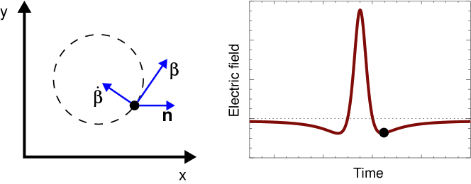
Figure 7.1: The path of a charged particle moving in a homogenous magnetic field (left panel). The particle radiates a time dependent electric field. An observer situated at great distance along the $\mathrm{n}$-vector sees the retarded electric field from the gyrating particle (right panel). As a result of relativistic beaming, the field is seen as pulses peaking when the particle moves directly towards the observer.

The derivation from here to obtaining an expression for the emitted radiation as a function of frequency is rather extensive (Jackson, 1999). In appendix C, we follow this derivation with the extension of including the full angular dependency and we find the following result

$$\frac{d^{2}W_{\perp}}{d\omega d\Omega} = \frac{\mu_{0}cq^{2}\omega^{2}}{12\pi^{3}}\left(\frac{r_{L}\theta_{\beta}\sin\theta}{c}\right)^{2}\frac{\left|K_{\frac{1}{3}}\left(\chi/\sqrt{\cos\theta\beta^{3}}\right)\right|^{2}}{(\cos\theta\beta^{3})}$$ (7.9)

$$\frac{d^{2}W_{\parallel}}{d\omega d\Omega} = \frac{\mu_{0}cq^{2}\omega^{2}}{12\pi^{3}}\left(\frac{r_{L}\theta_{\beta}^{2}\beta^{2}}{c}\right)^{2}\frac{\left|K_{\frac{2}{3}}\left(\chi/\sqrt{\cos\theta\beta^{3}}\right)\right|^{2}}{(\cos\theta\beta^{3})^{2}},$$ (7.10)

where $\theta$ is the angle between $\mathrm{n}$ and the orbital plane $\theta_{\beta}^{2}\equiv 2(1-\beta\cos\theta)$, $\chi=\omega r_{L}\theta_{\beta}^{3}/(3c)$ and $r_{L}$ the gyro-radius $\gamma mv/(qB)$. For $\beta\to 1$ and $\theta\to 0$, this expression converges toward the solution one normally find in text books (Jackson, 1999; Rybicki and Lightman, 1979).

We restrict the solution to $\cos\theta>0$. This is justified in the relativistic limit since the radiation from even mildly relativistic particles is beamed into a narrow cone around the velocity vector. Equation 7.9 and Eq. 7.10 describe the synchrotron radiation spectrum as observed in the orbital plane. At low frequencies it has a characteristic power-law slope of $\omega=2/3$. Above some critical frequency it drops of as $\omega e^{-k\omega}$.

Figure 7.1 shows the electrical field $\mbox{\boldmath$\mathrm{E}$}(t)$ from a particle that gyrates in a homogenous magnetic field as measured by an observer situated at great distance in the direction along $\mathrm{n}$.

7.2 Obtaining spectra from PIC simulations

In general, the approximations above will not be entirely accurate. In the PIC simulations (and in the ”real world”), the morphology of the electromagnetic field is often complicated, with a non-vanishing electric field. In this case, the paths of the particles are neither circular nor necessarily periodic. To obtain spectra from the simulations we need to take another approach. By sampling positions, velocities and accelerations from the simulation over a suitable time interval we can numerically evaluate the Fourier integral. First, we have to choose in which time frame we perform this integration: ”proper” time $t$ or retarded time $t^{\prime}$. The corresponding integrals are given in Eq. 7.4 and Eq. 7.8. At a first glance, Eq. 7.4 appears the most appealing since here we can use the standard Fast Fourier Transform (FFT) method, which is numerically faster. However, the term $(1-\mbox{\boldmath$\mathrm{\beta\cdot n}$})$ is numerically ill-behaved, and Eq. 7.4 has a higher power dependency on this term than Eq. 7.8. Furthermore, for a relativistic particle moving towards the observer, all features in the emitted radiation appear strongly contracted in the $t$-frame and are thus considerably harder to resolve numerically. Finally, in order to use an FFT, the numerical representation of $\omega$ needs to have uniform spacing, which is an inconvenient limitation. .

Before we proceed, several other numerical issues need to be considered.

7.2.1 Resolution constraints

Several issues should be kept in mind when implementing the time integration of the retarded signal. Constraints exist that are tied to the uncertainty relation

$$\Delta\omega\Delta t>1.$$ (7.11)

As explained by Rybicki and Lightman (1979) ”this uncertainty relation is not necessarily quantum in nature, but is a property of any wave theory of light”. As a result of this, the maximum frequency that can be represented in the resulting spectrum is limited by the number of points that one samples in a given time interval. This maximum frequency is known as the Nyquist frequency and equals half the sampling frequency (e.g. Press et al. 1986). It corresponds to a rapid oscillating signal that repeats once per two sample points in the time domain. Above the Nyquist frequency, the solution becomes aliased, noisy, and in general invalid (see Fig. 7.2 and Fig. 7.3). Thus, we set an upper limit on the frequency band to

$$\omega_{N}=\frac{1}{2\Delta t},$$ (7.12)

where $\Delta t$ is the time between each sample point. The low end of the frequency band is also limited since the lowest frequency that can be represented is that of a wave that repeats only once in the whole time interval. In fact, we must sample for long enough to detect not only low frequencies in the signal, but also small differences between frequencies (the resolution). Thus, the length of time for which we sample the signal ($T_{s}$) determines our ability to resolve differences between frequencies. This defines the frequency resolution

$$\Delta\omega=\frac{1}{T_{s}}.$$ (7.13)

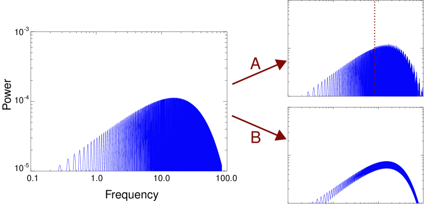
Figure 7.2: The observed power spectrum from a single charged particle, gyrating in a magnetic field (left panel). Case A: Reducing the sample rate distorts the frequencies above the Nyquist frequency, marked by a vertical dotted line. Case B: If the total time interval becomes too small (smaller than the orbit period) the main frequency lobes become smeared out. The units on the axis are arbitrary.

The effect of a too short total time interval can be seen from Fig. 7.2. Here we see that the individual spikes in the synchrotron spectrum are broadened out. So as a rule of thumb, the total length of the time sample should be at least one over the lowest gyro-frequency in the particle ensemble for which we wish to obtain a spectrum. For an ensemble of, say, thermal particles this poses a lesser problem, since the individual frequency peaks become averaged out to a continuum anyway.

Figure 7.3: An example of a numerical artifact introduced when trying to extend the spectrum to above the Nyquist frequency (dotted line). The effect is know as aliasing. The example spectrum is from electrons participating in the Weibel two-stream instability.

7.2.2 Time domain windowing

To determine the radiation power spectrum from an accelerated charged particle we sample the position, velocity and acceleration over a given time interval $T_{s}=t_{2}-t_{1}$. However, even for periodic orbits we cannot presume that this time interval is an integer number times the orbital period. And in the general case of sampling many particles over the time interval, in an inhomogeneous electromagnetic field, there will most certainly be a high level of a non-periodicity. However, the theory behind Fourier transformations assumes that the signal being processed is a periodic waveform. Connecting the ends of non-periodic signal introduces a discontinuity in the signal. Such a discontinuity in the time-domain can only be represented by a superposition of all frequencies in the frequency domain. The result is that any peak frequency (main lobe) is smeared out over a frequency range and side lobes occur around the main lobe. This is known as spectral leakage (e.g. Press et al. 1986). From experiments we have found that this leakage can alter the characteristic $\omega^{2/3}$ slope in the spectrum from a single synchrotron particle.

Figure 7.4: Windowing of a signal sampled over a time block ensures that the signal becomes periodic and continuous in the end points. This greatly reduces the spectral leakage.

To solve this problem, we apply a filtering function on the time dependent signal, to ensure that the signal becomes exactly zero in the end points of the chosen time sample block (and thus periodic), so that they match up and the transition is continuous (Fig. 7.4). The technique is known as windowing and is a standard tool in discrete signal analysis. The choice of window function depends on the problem. Several standard functions exist (Hanning, Hamming, Kaiser-Bessel…). After trying several of these, as well as other functions on the synchrotron radiation case we have found a good ad hoc window function

$$W(t)={\mathrm{Exp}}\left[-\left(k\frac{t-{\small\frac{1}{2}}(t_{1}+t_{2})}{t_{2}-t_{1}}\right)^{m}\right]$$ (7.14)

with the parameters $k=3$ and $m=6$.

After applying a window function to the signal it is important to renormalize the sample in order to retain the amplitude of the spectrum. Thus we multiply the final spectrum with the factor $A_{W}^{2}$ where

$$A_{W}=\frac{(t_{2}-t_{1})}{\int_{t1}^{t2}W(t)dt}.$$ (7.15)

With the window function applied on the sampled data, the expected $\omega^{2/3}$ synchrotron slope is effectively restored.

Figure 7.5: To obtain a spectrum from the PIC simulation at time $t$, particles are traced over a time interval around $t$ with high temporal resolution. Positions, velocities, and accelerations are sampled and from equation 7.8 we find the radiation spectrum.

7.2.3 Implementation and testing

The procedure above has been implemented in two steps. The first part is to sample position, velocity and acceleration for each particle. In general, one could dump particle data directly from the simulations. This, however, requires not only vast amount of disk storage, but one also needs to run the simulations with a time step much smaller than otherwise needed. The reason for this is discussed in Section 7.2.1. Typically, the time step in the spectrum tracer is of the order of 100 times smaller than in the PIC code. Since the simulations already take several weeks to run, we choose to take another approach (Fig. 7.5): When a simulation has finished, we choose a snapshot for which we want to obtain the radiation spectrum. Loading fields and particles from the chosen time step, we trace a given number of the particles back and forth in a time segment with very high temporal resolution, while keeping the electromagnetic fields frozen. In this sense, the particles can be seen as test particles. At each small time step we then store the particle positions, velocities and accelerations in a file. This data is read by another program that evaluates the Fourier integral (in the retarded time frame) given a direction $\mathrm{n}$ towards the observer. Finally we add the spectrum of each particle into a total spectrum. Adding the spectra from each particle linearly is valid as long as the phase of each contribution is completely uncorrelated to the others. This is clearly an assumption, which would be violated for example in a maser arrangement. The spectrum may finally be Lorentz/Dobbler boosted to any observer rest frame.

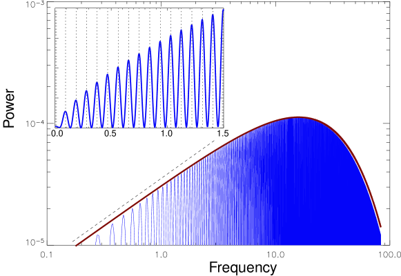
Figure 7.6: The spectrum obtained from a single particle gyrating in a magnetic field from the code (blue). The thick red line shows the theoretical synchrotron spectrum. The dashed line indicates the power-law slope $2/3$. The inset in the upper left corner shows that the spectrum consists of a discrete set of spikes that are integer overtones of the gyrofrequency, in this case $\omega_{B}=0.094$ (arbitrary units) (dotted vertical lines). The particle has a Lorentz factor $\gamma=5$. All numbers are in simulations units.

Test: Synchrotron radiation

To verify the ability of radiation code to produce correct spectra from accelerated charges, a series of tests have been performed. The first test is that of synchrotron radiation. We place a single relativistic particle in a homogeneous magnetic field (Fig. 7.1). The theory predicts that the emitted energy spectrum should consist of a collection of peaks, positioned at the gyro-frequency and higher harmonics. The amplitude of the individual peaks follow the continuum profile given by Eq. 7.10. Fig. 7.6 shows the spectrum we obtain from the code for a single relativistic charged particle in a homogenous magnetic field. We find very good agreement between the spectrum obtained from the simulation (blue line) and the theoretical synchrotron spectrum from Eq. 7.10 (red line). As expected, the peaks are found at harmonics of the gyro eigenfrequency and the low energy part follows a power-law slope $\omega^{2/3}$.

If one observes not a single synchrotron particle, but rather a whole ensemble of particles, the characteristics of the spectrum change. If all the particles in the ensemble have the same energy, but have momentum vectors that are isotropic distributed, the characteristic low-energy power-law slope of the integrated spectrum is altered. Integrating Eq. 7.9 and 7.10 over all pitch angles yields a spectrum with a low-energy part of the spectrum that has a power-law slope of $1/3$ rather than $2/3$ (Rybicki and Lightman, 1979). The results from the simulations are in excellent agreements with this. Figure 7.7 shows the spectrum from 512 particles, sampled from a mono-energetic distribution function ($\gamma=10$).

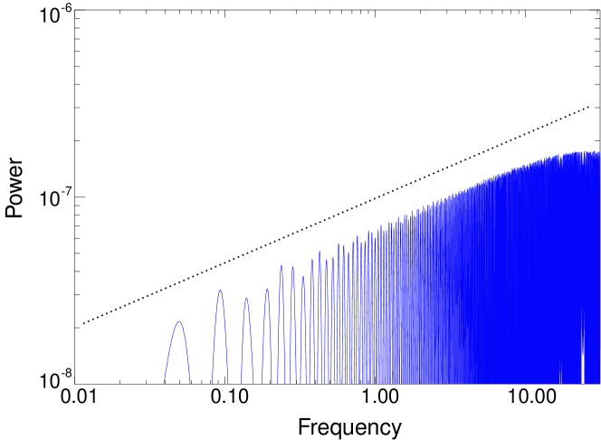
Figure 7.7: The low energy part of the spectrum from an ensemble of electrons with $\gamma=10$ and random orientation of the momentum vector. The ensemble is placed in a homogeneous magnetic field. The dotted line indicates a power law slope of 1/3. 512 particles were traced for this spectrum.

Test: Bremsstrahlung

Another important test that our radiation tool must pass is to reproduce the theoretically predicted spectrum of bremsstrahlung. Bremsstrahlung is emitted when the path of a charged particle is perturbed by an electric field (e.g. an ion). In the present version of the PIC code (and in most other PIC codes), the particles cannot interact directly but only through the grid. For simulations where each cell in the computational domain is quasi-neutral, bremsstrahlung is not included. The next generation of out PIC code will be able to include particle-particle interactions to some extent (see Chapter 8). We can, however, still test the radiation module by placing a single ion/electron pair in a simulation box.

Where synchrotron radiation is a periodic phenomenon tied to a magnetic field, bremsstrahlung is non-periodic and connected to electric deflections. So in a sense, this test complements the synchrotron test very nicely.

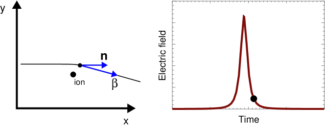
Figure 7.8: A relativistic electron passes an ion (left frame). The electrical far-field peaks as the electron is accelerated by the ion (right frame).

Figure 7.8 shows the example setup where an electron passes an ion and becomes subject to acceleration. In the relativistic limit the theoretical spectrum for this process may be derived using the beautiful theory of virtual photons (Rybicki and Lightman, 1979): In the rest frame of the electron, the electric field from the ion appears as a short, Lorentz contracted, electromagnetic pulse that can be view as a virtual photon. This virtual photon Compton scatters of the electron to produce the emitted radiation. Transforming back to the lab frame of the ion gives the relativistic bremsstrahlung emission from the electron

$$\frac{W_{\perp}}{d\omega}=\frac{q^{6}Z^{2}}{24\pi^{4}\epsilon^{3}c^{3}m^{2}v^{2}b^{2}}\left(\frac{\omega b}{v\gamma^{2}}\right)^{2}K_{1}^{2}\left(\frac{\omega b}{v\gamma^{2}}\right).$$ (7.16)

Here, $Z$ is the number of charges in the ion, $b$ is the minimum distance between that ion and the electron and $K_{1}$ is the modified Bessel function of the second kind. We note that a factor of $K_{1}$ is missing in Eq. 5.23 on page 164 in Rybicki and Lightman (1979). In Eq. 7.16, the $\perp$ indicates that we have neglected the contribution from the component of the ions electric field that is parallel to the path of the incoming electron. This approximation is valid in the ultra relativistic limit ($\gamma\gg 1$). Figure 7.9 shows the simulation results (thick blue) compared with Eq. 7.16 (thin red) for different electron energies ($\gamma v$=0.5, 2.5, 5.0, 7.5, 10.0). We find good agreement between simulations and the theoretical result for $\gamma v>1$. The deviation for $\gamma\to 1$ is because of the approximation in Eq. 7.16 above.

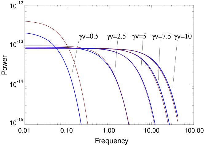
Figure 7.9: The theoretical (thin red) and simulated (thick blue) bremsstrahlung spectrum from an electron passing an ion. Four cases have been tested, differing only in initial electron energy (relativistic momentum $\gamma v$=0.5, 2.5, 5, 7.5, 10).

Test: Undulator radiation

A final but crucial test is whether the radiation code can reproduce the spectrum from undulator radiation. Undulator radiation is emitted when a relativistic electron traverses a periodic magnetic field so weak that the deflection angle stays within the relativistic beaming cone. The phenomenon is well known, and widely used, in synchrotron storage ring experiments. Figure 7.10 shows a schematic view of the generation of undulator radiation (Attwood et al., 1993). A full introduction to the field of undulator and wiggler radiation is given by Attwood (2000).

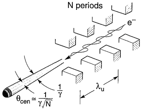
Figure 7.10: A schematic view of a undulator experiment in a cylotron. A cluster of magnets are aligned along the path of the electron. When the electron passes the array of magnetic, it radiates at the undulator frequency. From Attwood et al. (1993)

The spectrum from a relativistic electron moving in a transverse periodic undulator field (with magnetic wavelength $\lambda_{u}$ and maximum strength $B_{0}$), is characterized by a well confined peak near $\omega_{u}$, determined by the undulator equation (Kincaid, 1977)

$$\omega_{u}=\frac{2c\gamma^{2}}{\lambda_{u}(1+K^{2}/2+\gamma^{2}\theta_{u}^{2})}.$$ (7.17)

Here, $\theta_{u}$ is the angle between the path of the electron and the line of sight and $K$ is the periodic magnet parameter, defined as

$$K=\lambda_{u}qB_{0}/(2\pi m_{e}c).$$ (7.18)

In the weak-field case ($K<1$) the deflection angle of the undulation is smaller than the beaming opening angle $1/\gamma$ and the radiation is confined into the angle $1/\gamma$. For $K>1$ the radiation (called wiggler radiation) is emitted into a cone of half-angle $K/\gamma$. In this section we focus on $K<1$. The width of the peak is determined by how many periods $N$ the electron path is sampled over. The more undulations, the better defined the peak becomes.

Figure 7.11 shows the result of simulations where a single, relativistic electron ($\gamma=10$) moves in a periodic magnetic field. The undulator wavelength is $\lambda_{u}=11$ grid-zones and the periodic magnet parameter $K=0.0015$ (Eq. 7.18). The four panels in the figure represent different angles between the electron path and the line of sight ($\theta_{u}$=0, 0.01, 0.05, and 0.1). As expected (Attwood, 2000) the spectrum peaks at the frequency given by Eq. 7.17 (dotted lines). As $\theta_{u}$ is increased, higher harmonics of $\omega_{u}$ becomes visible. We thus find excellent agreement between the undulator equation Eq. 7.17 and the simulations.

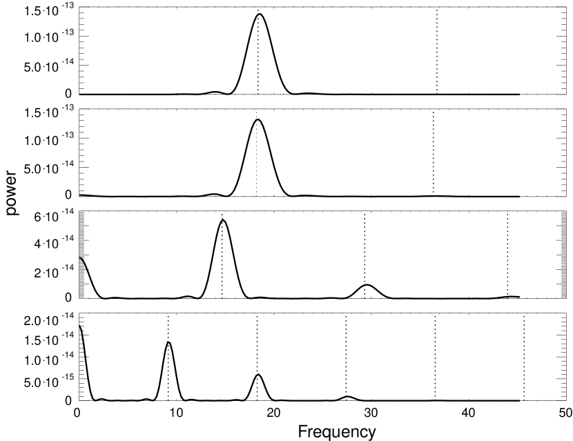
Figure 7.11: Undulator spectra generated when a $\gamma=10$ electron traverses a periodic magnetic field. The spectra are obtained from simulations with different viewing angles $\theta_{u}$= 0, 0.01, 0.05, and 0.1 (top to bottom panel). The dotted lines show the expected undulator frequency $\omega_{u}$ and its higher harmonics.

7.3 Jitter radiation

After having tested the radiation generation module thoroughly, we now focus on some more scientific issues. The PIC plasma simulation code, in combination with the radiation generation module, provides us with a powerful tool for testing various non-linear problems.

We choose to address several problems, all connected to the theory of 3D jitter-radiation from GRB plasma shocks. Jitter radiation was introduced to the GRB community by Medvedev (2000). It covers the regime where the magnetic field is inhomogeneous on scales smaller than the Larmor radius (see Fig. 7.12) and the electron’s transverse deflections in these fields are much smaller than the relativistic beaming angle. The foundation and motivation for such a theory was based on the small-scale nature of the magnetic fields generated by the two-stream instability. In the one-dimensional analytical approach, Medvedev (2000) found that the low frequency slope of the spectrum could be steeper than the $1/3$ slope of synchrotron radiation.

Figure 7.12: An example of the complicated paths of the electrons under the influence of electromagnetic field generated by the Weibel two-stream instability.

In this section, we first perform a parameter study to investigate the nature of the radiation emitted from an ensemble of relativistic electrons in different small-scale magnetic configurations (all with $K<1$).

Secondly, we compare the radiation that is emitted from a electron population in a generic, turbulent magnetic field (power-law distributed power-spectrum) with a two-stream generated magnetic field obtained from a snapshot from the PIC simulations. The question is: Is it reasonable to apply the theory of jitter-radiation directly on GRB shocks, assuming some generic structure of the magnetic field or must one include the complicated spatial details of a two-stream generated magnetic field? Our concern is that the ordered sub-structures in the two-stream generated magnetic field may affect the radiation spectrum.

Figure 7.13: 2D-slices of a turbulent magnetic field for three different values of the spectral power law index $\mu$: $\mu=-2$ (red noise, top), $\mu=0$ (white noise, middle) and $\mu=2$ (blue noise, bottom).

7.3.1 The 3D jitter spectrum

Jitter radiation is in family with undulator radiation, except that the magnetic field has power in many Fourier harmonics rather than only one, and in general follows a power-law in Fourier space. We define the power-spectrum of the magnetic field

$$P_{B}(k)=C_{B}k^{\mu}$$ (7.19)

(note that Medvedev (2000) defines the spectrum as $B_{k}=C_{B}k^{\mu}$, which means that there is a factor 2 difference on $\mu$ compared to our definition). In the original calculations, Medvedev (2000) assumed that $\mu\geq 1$. However, large-scale PIC-simulations (e.g. Frederiksen et al. (2004)) have shown that the magnetic field generated by the non-linear Weibel two-stream instability is indeed power-law distributed but has $\mu<0$.

Figure 7.14: The jitter spectra from a mono-energetic ensemble of electrons ($\gamma=3$) moving in a turbulent magnetic field. The different graphs are for simulations with different values of $\mu$. The amplitude of the magnetic field is set so that the periodic magnet parameter $K<1$ for all $k$-nodes (Eq. 7.18).

In this section we investigate the radiation from an ensemble of relativistic electrons, moving in a random magnetic field, for different values of the spectral power law index $\mu$ (see Fig. 7.13). The result is a three-dimensional generalization of the jitter-theory that differs substantially from the one-dimensional result found by Medvedev (2000). In this thesis, we do not include the regime where an additional large-scale amplitude field is present (Medvedev, 2000).

We have performed simulations of an isotropic mono-energetic ensemble of electrons ($\gamma=5$). The isotropic distributions may be seen as an integration over all angles of the undulator equation. The electrons are placed in a simulation box with $200\times 200\times 800$ grid-zones with a turbulent magnetic field that has a Fourier distribution as in Eq. 7.19. Seven different values of $\mu$ have been examined. The amplitude of the magnetic field is set so that the mean magnetic field energy is the same in each simulation. The periodic magnet parameter $K$ is less than 1 for all Fourier nodes. The range of the power-law is limited to $k_{min}<k<k_{max}$ where $k_{min}$ and $k_{max}$ correspond to minimum and maximum frequencies that can be represented by the simulation grid (Fig. 7.13).

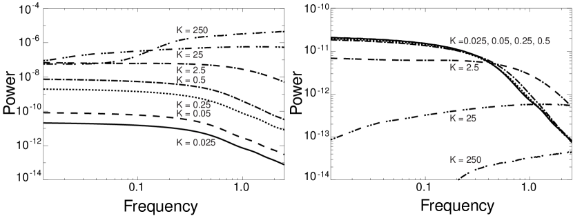
Figure 7.15: Increasing the magnetic field increases the magnet parameter $K$ (Eq. 7.18). The left panel shows how the amplitude of the undulator spectrum increases with $\langle B^{2}\rangle$. When $K$ becomes larger than 1, a transition to the wiggler radiation spectrum occurs. The right panel shows the same spectra divided with $\langle B^{2}\rangle$.

The resulting 3D jitter radiation spectrum from the electrons can be seen in Fig. 7.14. Quite interestingly, all the spectra have similarity with the bremsstrahlung spectrum for low energies (flat spectrum). At higher energies, the $\mu>0$ cases drop off very sharply – faster than the bremsstrahlung spectrum. For $\mu<0$ the high-energy part of the spectrum is found empirically to be a power-law with a slope of $\omega^{\mu-1}$. The reason why the $\mu>0$ peaks at so much higher frequencies than for $\mu<0$ can be understood from Eq. 7.17, which shows that the characteristic frequency scales as $k$ ($\sim 1/\lambda_{u}$).

We have also tested how the spectrum depends on the magnetic field amplitude. From Fig. 7.15 we find that the amplitude scales with $B^{2}$ as expected from Larmor’s radiation formula. Above the limit where the deflection angle becomes comparable to, or larger than the beaming angle ($K>1$), the spectrum enters the wiggler-domain. The wiggler radiation spectrum is close to the synchrotron spectrum (Attwood, 2000).

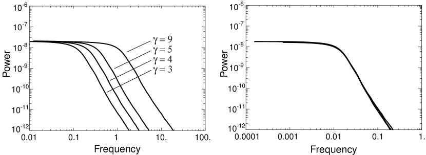
Figure 7.16: The radiation spectrum from four different mono-energetic ensembles of electrons ($\gamma$=3, 4, 5, and 9) with isotropic distributed momentum-vectors, placed in a turbulent magnetic field with spectral slope $\mu=-3$ (left panel). The right panel shows the same four graphs but shifted in frequency with a factor $\gamma^{-2}$ (renormalized).

We finally test the $\gamma$-dependency. Figure 7.16 and Fig. 7.17 show the jitter radiation spectra for $\mu<0$ and $\mu>0$ for electron ensembles with different energies. Even though the spectra in the two cases differ, they both scale the same way: The spectra are shifted with $\gamma^{2}$ in frequency in agreement with Eq. 2.9 (and Eq. 7.17).

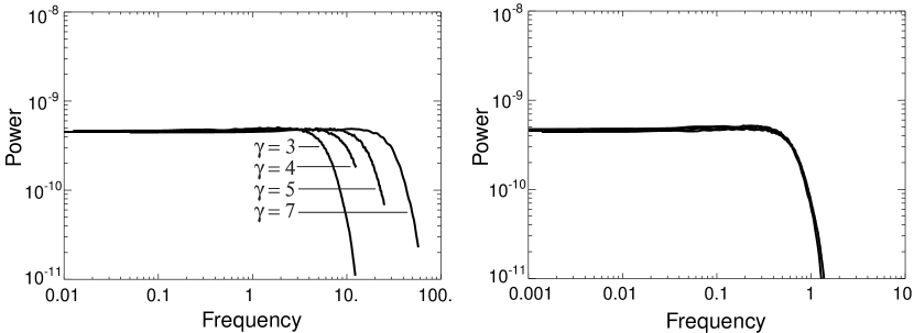
Figure 7.17: The radiation spectrum from four different mono-energetic ensembles of electrons ($\gamma$=3, 4, 5, and 7) with isotropic distributed momentum vectors, placed in a turbulent magnetic field with spectral slope $\mu=+3$ (left panel). The right panel shows the same four graphs but shifted in frequency with a factor $\gamma^{-2}$ (renormalized).

7.3.2 Jitter radiation from collisionless plasma shocks?

In this section, we compare the radiation spectrum from an ensemble of electrons, moving in two different magnetic topologies: 1) the magnetic field generated by the Weibel two-stream magnetic field $\mbox{\boldmath$\mathrm{B}$}_{0}$ (see Section 3 in this thesis, Medvedev and Loeb 1999 and Frederiksen et al. 2004) and 2) a randomized magnetic field $\mbox{\boldmath$\mathrm{B}$}_{1}$ that has the same average energy density and spectral power spectrum as the two-stream generated field. The purpose of this exercise is to test if there are any differences in the resulting radiation spectra. $\mbox{\boldmath$\mathrm{B}$}_{0}$ is readily available from the PIC simulations. Constructing $\mbox{\boldmath$\mathrm{B}$}_{1}$ is more tricky. To make sure that $\mbox{\boldmath$\mathrm{B}$}_{1}$ has exactly the same average energy density and power spectrum properties as the PIC-field $\mbox{\boldmath$\mathrm{B}$}_{0}$, we generate the random field in the following way:

The basic idea is to Fourier transform the magnetic field from $\mbox{\boldmath$\mathrm{B}$}_{0}$, make a random phase shift of all $k$-nodes in the Fourier domain and then transform back to real-space. This is easily done but has one serious flaw: we cannot be sure that the resulting magnetic field obeys $\nabla\cdot\mbox{\boldmath$\mathrm{B}$}_{1}=0$ even though $\mbox{\boldmath$\mathrm{B}$}_{0}$ does. The solution is to work on the vector potential rather than directly on $\mbox{\boldmath$\mathrm{B}$}_{0}$. The vector potential $\mbox{\boldmath$\mathrm{A}$}_{0}$ is a vector field that satisfies $\mbox{\boldmath$\mathrm{B}$}_{0}=\nabla\times\mbox{\boldmath$\mathrm{A}$}_{0}$. Inverting this equation requires $\mbox{\boldmath$\mathrm{B}$}_{0}$ to be periodic. In the PIC simulations, $\mbox{\boldmath$\mathrm{B}$}_{0}$ is already periodic in the two-dimensions perpendicular to the jet flow ($x,y$). To make the magnetic field periodic in the $z$-direction we apply a windowing function that connects the magnetic field-lines through the $z$-boundary. Away from the boundary, the magnetic field remains unchanged. We have tested that this filter does not alter the power spectrum of $\mbox{\boldmath$\mathrm{B}$}_{0}$ except for a few percent in the very highest frequencies. Ensured that $\mbox{\boldmath$\mathrm{B}$}_{0}$ is periodic, the Fourier transform of $\mbox{\boldmath$\mathrm{A}$}_{0}$ into $\hat{\mbox{\boldmath$\mathrm{A}$}}_{0}$ is

$$\hat{\mbox{\boldmath$\mathrm{A}$}}_{0}(\mbox{\boldmath$\mathrm{k}$})\equiv\mathrm{FFT}(\mbox{\boldmath$\mathrm{A}$}_{0})=i\mbox{\boldmath$\mathrm{k}$}\times\mathrm{FFT}(\mbox{\boldmath$\mathrm{B}$}_{0})/|\mbox{\boldmath$\mathrm{k}$}|^{2}.$$ (7.20)

$\mathrm{k}$ is the wave vector and FFT represent a fast Fourier transformation.

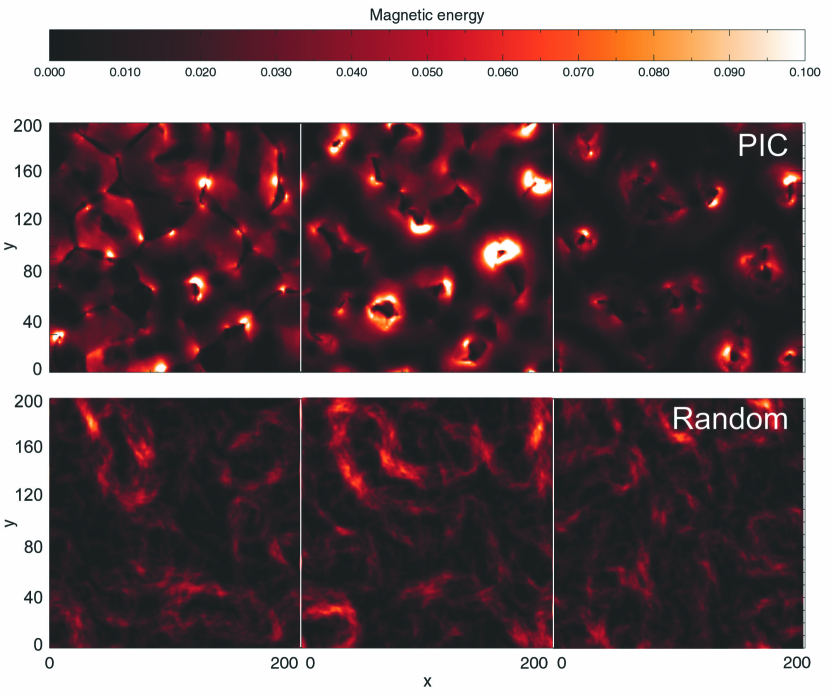
Figure 7.18: The spatial distribution of magnetic energy in three slices sampled at different depth in the plasma shock. The top panel shows $\mbox{\boldmath$\mathrm{B}$}_{0}$ generated by the two-stream instability. The lower panel shows a random magnetic field $\mbox{\boldmath$\mathrm{B}$}_{1}$ with the same spectral power distribution as $\mbox{\boldmath$\mathrm{B}$}_{0}$.

We then scramble the vector potential by a random phase shift of all the Fourier harmonics

$$\hat{\mbox{\boldmath$\mathrm{A}$}}_{1}(\mbox{\boldmath$\mathrm{k}$})=\hat{\mbox{\boldmath$\mathrm{A}$}}_{0}(\mbox{\boldmath$\mathrm{k}$})e^{i2\pi\mbox{\boldmath$\mathrm{k}$}\tilde{f}},$$ (7.21)

where $\tilde{f}$ is a matrix of random numbers in the range $[0;1]$. The size of $\tilde{f}$ matches the total number of data points in the three-dimensional ${\mbox{\boldmath$\mathrm{B}$}}_{0}$-array. $\mbox{\boldmath$\mathrm{B}$}_{1}$ is then given as $\mbox{\boldmath$\mathrm{B}$}_{1}=\nabla\times\mbox{\boldmath$\mathrm{A}$}_{1}$. The transformation is performed in IDL (Interactive Data Language by Research Systems Inc.) and this adds a few complications to the process, mainly connected to the representation and renormalization of the Fourier transforms. To ensure that no errors have been introduced in the process of obtaining $\mbox{\boldmath$\mathrm{B}$}_{1}$, we check and find that

• $\mbox{\boldmath$\mathrm{B}$}_{0}$ and $\mbox{\boldmath$\mathrm{B}$}_{1}$ have identical Fourier transforms and equivalently, identical spectral power distribution,

• $\mbox{\boldmath$\mathrm{B}$}_{1}$ is real if $\mbox{\boldmath$\mathrm{B}$}_{0}$ is real,

• the magnetic energy is conserved through the transformation $\int\mbox{\boldmath$\mathrm{B}$}_{1}^{2}dV=\int\mbox{\boldmath$\mathrm{B}$}_{0}^{2}dV$, and

• $\mbox{\boldmath$\mathrm{B}$}_{1}$ is divergence free ($\nabla\cdot\mbox{\boldmath$\mathrm{B}$}_{1}=0$).

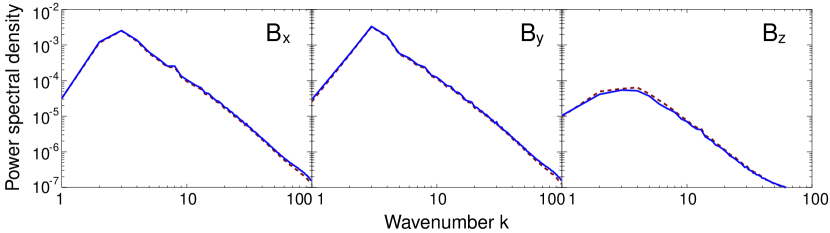
Figure 7.19: Power spectrum of the magnetic field generated by the Weibel two-stream instability $\mbox{\boldmath$\mathrm{B}$}_{0}$ (full line) and the random phase shifted field $\mbox{\boldmath$\mathrm{B}$}_{1}$ (dotted line).

Figure 7.18 shows the input magnetic field $\mbox{\boldmath$\mathrm{B}$}_{0}$ and the resulting $\mbox{\boldmath$\mathrm{B}$}_{1}$. Three slices are shown for each field, sampled at different depths in the shock. Figure 7.19 shows the power spectrum of $\mbox{\boldmath$\mathrm{B}$}_{0}$ and $\mbox{\boldmath$\mathrm{B}$}_{1}$. Clearly, the randomized magnetic field $\mbox{\boldmath$\mathrm{B}$}_{1}$ has the same statistical characteristics as the magnetic field from the simulations.

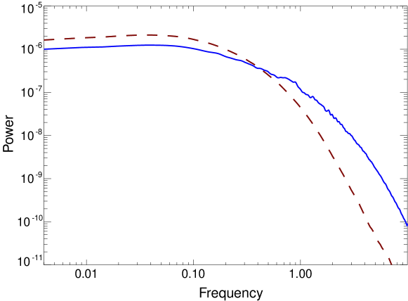
Figure 7.20: Radiation from PIC simulations (solid blue) compared to radiation from a random field with the same statistical properties (dashed red). Both spectra are generated by using the same ensemble of 20000 electrons.

In Fig. 7.20 we compare the radiation spectrum from a thermal electron ensemble in $\mbox{\boldmath$\mathrm{B}$}_{0}$, with the spectrum of the same ensemble in $\mbox{\boldmath$\mathrm{B}$}_{1}$. $\mbox{\boldmath$\mathrm{B}$}_{0}$ is from PIC simulations of a plasma shock ($\Gamma=3$ simulation from Chapter 3). $\mbox{\boldmath$\mathrm{B}$}_{1}$ is created as described above. Both spectra are generated by tracing 20000 electrons. To make the spectra as realistic as possible, the electron positions and velocities are sampled from a snapshot of the PIC simulation.

We find that the two spectra peak at the same frequency but diverge considerably for high frequencies where the radiation spectrum from the random field $\mbox{\boldmath$\mathrm{B}$}_{1}$ has a harder cutoff. The reason for this is because of the higher peak-values in the magnetic field from the PIC simulations (see Fig. 7.18). Even though $\mbox{\boldmath$\mathrm{B}$}_{0}$ and $\mbox{\boldmath$\mathrm{B}$}_{1}$ have the exact same power-spectrum, there exists phase-correlations in $\mbox{\boldmath$\mathrm{B}$}_{0}$ that give the field a more coherent structure ($\mbox{\boldmath$\mathrm{B}$}_{1}$ has a larger volume filling factor). We know also that the frequency where the synchrotron spectrum peaks $\nu_{c}$ scales linearly with the magnetic field strength. Finally, the high-energy electrons are primarily found near ion-current channels where the magnetic field peaks (see Fig. 3.1, 6.1 and 6.4). We conclude that it would appear that one may use a random magnetic field for analytical calculations, but only as a first approximation. We also stress that the simulation results we have used are from simulations that do not include the full shock ramp. The spectra may diverge even more for radiation from a full shock.

Radiation due to Electric Fields

Electric fields are most often neglected in generation of radiation from astrophysical shocks. In PIC simulations we have found that for collisionless shocks where the magnetic field is generated by the Weibel two-stream instability, electric fields exist with an energy density of the order of $10\%$ of the generated magnetic field. Figure 7.21 shows two radiation spectra emitted from a collisionless shock. The electron distribution and electromagnetic field that lie behind the radiation are taken directly from self-consistent PIC code simulations. The left panel of 7.21 shows a spectrum where only the magnetic field is taken into account, while the right panel shows the spectrum when the electric field is also included. For a pure magnetic field we immediately identify the wiggler/synchrotron signature from the $\omega^{1/3}$ low energy slope. The main effect from including the electric field is that the low energy slope is flattened to $\sim\omega^{1/6}$ and the high-energy exponential cut-off is softer and goes to higher energies. From these plots we conclude that it is important to also include the electric field generated in the Weibel two-stream instability.

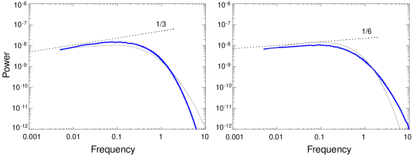
Figure 7.21: The spectrum of a mono-energetic ($\gamma=3$), isotropic electron population in the electromagnetic field generated by the Weibel two-stream instability. In the left panel, only the magnetic field is included whereas the right panel includes both the magnetic and electric field. The grey shaded line in the left panel is a copy of the spectrum in the right panel and visa verse. 20000 particles were traced in each spectrum. Both axis are in arbitrary units.

7.4 Spectra from the PIC simulations rescaled into ’real space’

The ultimate goal is to obtain spectra from the PIC shock simulations that can be compared directly to observations. Even though it is beyond the scope of this thesis, this will eventually allow us to put constraints on the physics of GRB afterglows.

In the PIC simulations, several parameters have been scaled to simulation units. To make the simulation results more directly comparable to real observations, it is necessary to correct for this. Rescaling the radiation spectra obtained from simulations involves several effects:

Simulation time-scales:

To rescale the time-scale of the simulations to real space, we must divide all frequencies with the plasma frequency in the upstream part of the simulation box $\omega_{p}^{\prime}$, and multiply with the real space (ISM) plasma frequency $\omega_{p}$. That is, we have to multiply with a factor $R_{1}=\omega_{p}/\omega_{p}^{\prime}$. In the non-linear phase of the Weibel two-stream instability, the ions are dominating the evolution of the instability. Therefore, we set $\omega_{p}^{\prime}$ equal to the upstream ion plasma frequency from the simulations ($\omega_{p}^{\prime}=0.025$). Since we are focusing on the afterglow domain in the simulations, we choose the ion plasma frequency of the inter-stellar medium for the real space plasma frequency, ($\omega_{p}\simeq 1300\ \mathrm{s}^{-1}$). In this case, $R_{1}=1300/0.025\simeq 5\cdot 10^{4}$.

Ion to electron mass ratio:

For numerical convenience, the ion (proton) to electron mass ratio are rescaled (see Section 2). The ion/electron charge ratio remains unity. From the simulations it is found that the ions dominate the Weibel two-stream instability. Therefore, we can see the mass rescaling as an unphysical rescaling of the electron mass/charge ratio. In the code, the ion/electron mass ratio is typically 16. Using the real mass ration 1836 would mean that the electrons become accelerated to higher Lorentz factors (but the same energy) by a factor 1836/16. In Section 7.3.1 we found that the peak frequency in the spectra scales with $\gamma^{2}$. This is consistent with synchrotron radiation (Rybicki and Lightman, 1979): In synchrotron radiation, the peak frequency is proportional to $\gamma^{2}/m_{e}$. Thus we must effectively shift the radiation spectrum up in frequency by a factor $R_{2}=(1836/16)^{3}=1.5\cdot 10^{6}$

Relativistic Doppler shift:

All the simulations are carried out in the rest frame of the shock, moving with a bulk lorentz factor $\Gamma$ towards the observer (only GRB jets moving directly towards us will trigger the space telescopes as a result of the relativistic beaming). We must therefore shift the simulation radiation spectra with a relativistic Doppler correction term $R_{3}\simeq 2\Gamma$.

In summary, to compare the spectrum we have obtained from the simulations of a $\Gamma=15$ shock propagating through the ISM, we must shift the frequency axis with a factor $R=R_{1}R_{2}R_{3}\simeq 2\cdot 10^{12}$. This puts us somewhere near the optical frequency band. In Fig. 7.22 we show the radiated spectrum, sampled from 20.000 electrons. After applying the rescaling, we find that the spectrum peaks in the far infrared area. Below the peak, we find a power-law segment with slope $P(\omega)\propto\omega^{2/3}$. This is interesting because it is steeper than the synchrotron $1/3$ slope and thus might shed light on the issue about ”the line of death” (Preece et al., 1998) for many bursts. For frequencies above the peak frequency, the spectrum continues into the near infrared/optical band, following a power-law with slope $P(\omega)\propto\omega^{-\beta}$ with $\beta\simeq 0.7$.

From the power-law slope in the spectrum with ($\beta=0.7$), the standard procedure in the GRB community would find that the electrons have a power-law distribution, with slope $p=2.4$ (determined by solving $(p-1)/2=\beta$). The standard conclusion would be that this is consistent with Fermi acceleration. However, we strongly emphasize that the electrons that produced the spectrum in Fig. 7.22 are not Fermi accelerated. The electrons are instantaneously accelerated and decelerated in the highly complicated electric and magnetic field near the ion current channels under emission of strong radiation (see an example of the complicated electron-paths in Fig. 7.12). This differs substantially from the iterative acceleration in Fermi acceleration.

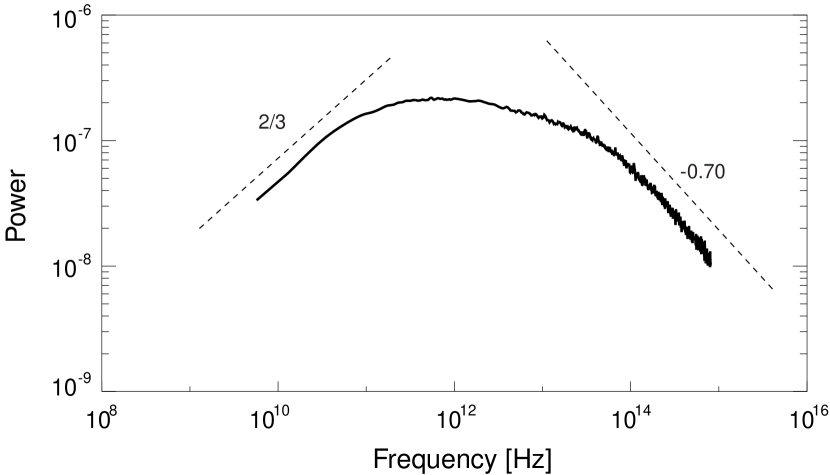
Figure 7.22: The spectrum from a $\Gamma=15$ plasma shock propagating into an ISM-like medium. The frequency scale is boosted in accordance with the physical arguments given in the text. The spectrum peaks in the far infrared. Below the peak, we find a power-law segment with slope $P(\omega)\propto\omega^{2/3}$. For frequencies above the peak frequency, the spectrum continues into the near infrared/optical band, following a power-law with slope $P(\omega)\propto\omega^{-\beta}$, where $\beta=0.7$.

We note that the box of the PIC simulation behind the spectrum presented in Fig. 7.22 is not large enough to cover the whole shock ramp (ions are not fully thermalized when they leave the simulation domain). This means that additional features might be added to the spectrum for even larger simulations. Moreover, the spectrum does not include synchrotron self-absorbtion.

7.5 Summary

I have developed, and tested, a tool can create radiation spectra directly from particle-in-cell simulations. By tracing particles, the code performs the exact radiation field Fourier integration (Eq. 7.8) without having to make assumptions about the magnetic field, particle orbit, beaming angle, and so forth.

The radiation tool has been thoroughly tested and successfully reproduces synchrotron radiation, bremsstrahlung, and undulator radiation from small-angle deflections.

I have used the tool to investigate the properties of three-dimensional jitter radiation in magnetic fields with different turbulent configurations. By tracing isotropic momentum distributions of electrons through a random magnetic field with a power spectrum that follows a power-law distribution in the Fourier domain $P_{B}(k)\propto k^{\mu}$, I have determined the resulting spectrum. I have focused on the weak field limit (where the deflection angle is less than the beaming cone angle, $K<1$). For all values of $\mu$, the radiation spectrum has a flat low-energy part (similar to bremsstrahlung). For $\mu<0$, the high-energy part of the spectrum follows a power-law with a slope $\alpha\simeq\mu-1$ independent of the electron energy. For $\mu>0$, the flat spectrum continues to higher frequencies than for $\mu<0$. The spectrum has a hard cut-off for high frequencies. With the present simulations, it is not possible to determine if the spectrum has peaks for even higher frequencies.

For all values of $\mu$ and $K<1$, the spectrum shifts in frequency with $\gamma^{2}$ and scales with the amplitude of the magnetic field squared $B^{2}$, in good agreement with Larmor’s formula for radiated power. In the limit of large deflections ($K>1$) the spectrum eventually converges through the wiggler spectrum to the ordinary synchrotron spectrum.

For all the spectra presented in this chapter, I have checked for convergence: For each spectrum obtained I have made a second run with twice the number of particles. If the two spectra have different shape, the process is repeated by doubling the particle number until the result converges. This process is important since radiation from high-energy particles is highly beamed. This is prone to distort the high-energy radiation spectrum because of bad statistic.

Computationally, the generation of spectra from simulations is not an easy task. One may say that it is an example where nature is not nice to scientists. Especially, obtaining a radiation spectrum from high-energy particles is not easy since it is necessary to integrate for a time period that grows linearly with $\gamma$ in order to sample at least a couple of orbits. But at the same time it is crucial to sample a very high number of time-steps per time unit, to resolve the peak in the electrical field, which is very narrow ($\gamma^{-2}$) because of relativistic beaming. So in total, the computational cost grows with $\gamma^{3}$. The good news is that each particle and frequency bin may be treated independently, which makes the problem embarrassingly parallel (in the jargon of High Performance Computing).

The method of tracing particles in an electromagnetic field that is fixed to a single snapshot is clearly an approximation. For high frequency spectra, this is not a problem, since we sample for a very short period of time. For low frequencies, it is a potentially more severe approximation since it doesn’t make sense to trace the particle for too long time in a field that would have changed significantly during this process. Improvements can be made in several ways. One method is to pick out a number of particles before the large simulation starts and then integrate these particles with a high number of sub-steps. Another approach would be to interpolate field values to the particles position not only in the spatial dimensions (which is already implemented) but also in time from different field snap shots.

An interesting step for the future is to determine the polarization in the synthetic spectra from the PIC simulations. Even though time did not allow for it in this thesis, it should not be difficult with the tools that are already developed. One could then investigate how the radiation spectrum, including polarization change as functions of the viewing angle measured from the jet propagation direction.

In the near future, the computational resources will reach a level where one can resolve fully three-dimensional collisionless shocks. It then becomes possible to make composite spectra from different simulations with varying bulk Lorentz factor as a function of viewing angle. This will allow us to test many interesting aspects with regard to jet structure and polarization predictions from shock-generated electromagnetic fields.

I end this chapter by emphasizing that strong magnetic field generation, particle acceleration and emission of non-thermal radiation are unavoidable consequences of the collision of two, initially unmagnetized, plasma shells.

Chapter 8 A next generation PIC code

8.1 Introduction

Over the last couple of years the Copenhagen group has been using PIC models that include electromagnetic fields and charged particles to understand the plasma microphysics of collisionless shocks Frederiksen et al. (2002, 2004); Hededal et al. (2004); Hededal and Nishikawa (2005). It has turned out to be a very successful tool, but it is still limited in the scope of phenomena that can be addressed. Even though a large class of astrophysical environments are indeed collisionless, scattering and collision processes do play an important role in several key scenarios. Examples are given below. Another key ingredient, which has been missing in charged particle simulations, is a full treatment of photon propagation. It can be argued that photons are represented directly on the mesh by electromagnetic waves, which certainly is correct. But the mesh can only represent waves with frequencies smaller than the Nyquist frequency. The physical length of a typical cell has in our applications typically been $10^{5}-10^{6}\ \textrm{cm}$ and hence it is clear that only low frequency radio waves can be represented. High-frequency photons have to be implemented as particles that propagate through the box and interact, either indirectly through messenger fields on the mesh, or directly with other particles. A valuable consequence of modelling the detailed photon transport is that extraction of electromagnetic spectra is trivial. Even in cases where the photon field is only a passive participant, this fact should not be underestimated as it enables direct comparison with observations.

There exists Monte Carlo based particle codes (see e.g. Stern et al. (1995) and references therein) that address various particle interactions, but one of their main shortcomings is the poor spatial resolution. This makes it impossible to couple the particle aspects to a self-consistent evolution of the plasma.

Our goal has been to develop a framework where both electromagnetic fields and scattering processes are included in a consistent way. We can then correctly model the plasma physics and the radiative dynamics. The scattering processes include, but are not limited to, simple particle-particle scattering, decay and annihilation/creation processes. Our new code is not limited in any way to charged particles, but can also include neutrals such as photons and neutrons.

In the next section we describe some of the physics that can be addressed with this new code. In section 8.2 we discuss how the code has been implemented, the general framework and in detail, which physical processes that are currently implemented. In section 8.3 we present the results of a preliminary toy experiment that we have performed to validate the code. In the last section 8.4 we summarize.

8.1.1 Motivation

Before we continue and describe in detail the methods, physics and test problems we have implemented and used, it is important to consider the general class of scenarios we have had in mind as motivation for developing the code. There are several key objects, where only the bulk dynamics is understood, and we are lacking detailed understanding of the microphysics.

Internal shocks in Gamma-Ray Bursts

In the internal/external GRB shock model, the burst of gamma-rays is believed to be generated when relativistic shells collide and dissipate their relative bulk energy Rees and Meszaros (1992); Meszaros and Rees (1993). The nature of the radiation is presumably inverse Compton scattering and synchrotron radiation. Particle/photon interactions might also play an important role in the very early afterglow as suggested by Thompson and Madau (2000); Beloborodov (2002): Even though the medium that surrounds the burst (ISM or wind) is optically very thin to gamma-rays, a tiny fraction of the gamma-rays will Compton scatter on the surrounding plasma particles. This opens up for the possibility of pair-creation between back scattered and outgoing gamma-rays. The creation of pairs may increase the rate of back scattered photons in a run-away process Stern (2003). The Compton scattering may accelerate the pair-plasma through the surrounding medium with many complicated and non-linear effects, including streaming plasma instabilities and electromagnetic field generation. Hence, it is crucial that plasma simulations of internal GRB plasma shocks include lepton-photon interactions.

Solar corona and the solar wind

Space weather (defined as the interaction of the solar wind on the Earth) is in high focus for several reasons. Not only is the Sun our closest star, providing us with invaluable data for stellar modelling, but also coronal mass ejections from the Sun potentially have impact on our every day life. The strong plasma outflows from the sun can induce large electrical discharges in the Earths ionosphere. This may disrupt the complex power grids on Earth, causing rolling blakcouts such as the one in Canada and North America in 1989. Also high-energy particles can be hazardous to astronauts and airline passengers. Computer simulations have provided a successful way of obtaining insight in these complex plasma physical processes. However, in the solar coronal and in the solar wind plasma out to distances beyond the earth orbit, difficulties arise in finding the right formalism to describe the plasma. Neither a collisionless model based on the Vlasov equation nor an MHD fluid model provides a adequate framework for investigation. The problem has already been studied using three dimensional PIC simulations but without taking collisions into account (e.g. Buneman et al. (1992); Hesse et al. (2001)).

The corona of compact objects

The bulk dynamics of accreting compact objects have been modelled for many years using fluid based simulations (e.g. Balbus (2003) and references therein). Nevertheless, it has been a persistent problem to extract information about the radiating processes. Furthermore in the corona the MHD approximation becomes dubious, just as in the solar corona. The environment around a compact object is much more energetic than the solar corona, and therefore radiative scattering processes play an important role. Pair production is also believed to be abundant. Using our new code it would be possible to model a small sub box of the corona. The main problem here – as in most numerical implementations – is to come up with realistic boundaries for the local model. A shearing box approach may be appropriate, but in fact we can do even better.

The size of a stellar mass black hole is around $10^{6}\ \textrm{cm}$. In a fluid simulation we want to model the accretion disk–compact object system out to hundreds of radii of the compact object. The normal approach is to use a non-uniform mesh. Nonetheless, the Courant criteria, which determines the time step, is still limited by the sound crossing time of the compact object. I.e. the time step is limited by the size of the innermost (and smallest) cells in the mesh. The very small time step corresponds to those found in a typical particle simulation, where the strict time step arises from the need to resolve plasma oscillations. Hence data from an MHD simulation could provide temporally well-resolved fluxes on the boundaries of the much smaller sub box containing the particle simulation.

In this sense the particle simulation will act as a probe or thermometer of the fluid model. The particle model includes the full microphysics in a realistic manner and most importantly includes photon transport. Realistic spectra could be obtained indirectly from the fluid model, testing fluid theory against observations. We have already started preliminary work on interfacing fluid models with the old PIC code.

Pre-acceleration in Cosmic Ray acceleration

Accepting Fermi acceleration as a viable mechanism for accelerating electrons and creating the non-thermal cosmic ray spectrum is still left with some big unanswered questions. One is that the Fermi mechanism requires injection of high-energy electrons while still keeping a large, low-energy population to sustain the magnetic turbulence. Hence, a pre-acceleration mechanism needs to be explained.

The shocks in supernova remnants are believed to be cosmic ray accelerators. However, the Fermi acceleration process in shocks is still not understood from first principles but rely on assumptions on the electromagnetic scattering mechanism. PIC codes would seem ideal in exploring the mechanism from first principles, since they include field generation mechanisms and the back-reaction that the high-energy particles have on this scattering agent. In Supernova remnants however, the mean free path for Coulomb collisions are comparable to the system and particle-particle interactions cannot be fully neglected.

8.2 Implementation

Implementing any state-of-the-art large-scale numerical code is a big undertaking, and can easily end up taking several man years. We estimate that the final version of the next generation code will contain more than 50.000 lines of code. Starting in February this year, it has taken us three man months to implement the current incarnation of the code, which has already grown to approximately 10.000 lines. Besides T. Haugbølle and C. B. Hededal, the development is done together with Å. Nordlund and J. T. Frederiksen. Fortunately we have a good tradition and expertise for numerical astrophysics in Copenhagen and we have been able to port different technical concepts and solutions from our suite of fluid codes and to a lesser extent from the old PIC code. The aim is to build an extremely scalable code that is able to run on thousands of CPUs on modern cluster architectures and utilize MPI as the inter node communication protocol. In this chapter we will not go further into technical details. Instead we will put emphasis on the important concepts and physics and how we have implemented these.

8.2.1 Concepts

The two fundamental objects in a particle-in-cell code are the mesh and the particles. We have adopted the solver and interpolation routines from the old PIC code to solve the Maxwell equations and find fluxes and densities on the mesh. The mesh is used to distribute messenger fields – such as the electromagnetic fields – and to calculate volume averaged fluxes and densities of the particles The latter are used as source terms in the evolution of the messenger fields. The particles really represent an ensemble of particles and are often referred to as pseudoparticles Birdsall and Langdon (1991) or large particles. A so-called smoothing kernel describes the density distribution of a single pseudoparticle on the mesh. In our implementation the volume of a particle is comparable to a cell in the mesh.

Pseudoparticles with variable weights

The concept of pseudoparticles is introduced since the “real space” particle density easily exceeds any number that is computationally reasonable (i.e. of the order of a billion particles). The pseudoparticle charge to mass ratio is kept the same as the ratio for a single particle.

In ordinary PIC codes the weight of each pseudoparticle of a given species is kept constant throughout the simulation. The benefit is a simple code and an unique identity for each particle. The first is a convenience in the practical implementation, the second important when understanding the detailed dynamics and history of a single particle.

Notwithstanding possible conveniences, as detailed below in section 8.2.1, we have decided to improve this concept to a more dynamical implementation where each pseudoparticle carries a individual weight. Particles are then allowed to merge and split up when a cell contains too many/few particles, or when particles are scattered. The concept is sometimes used in smooth particle hydrodynamics (SPH), where different techniques have been proposed for the splitting and merging of particles. It is both used to adjust the density of individual particles Børve et al. (2001) and in the conversion of gas– to star particles in galaxy formation models Governato et al. (2004). An important quality of SPH is its adaptive resolution capabilities. These are important in the description of collapsing self-gravitating systems, ranging from core collapse supernovae to the formation of galaxy clusters, scenarios where matter is collapsing many orders of magnitude, and therefore the smoothing length or volume of the individual particles is readjusted accordingly. Consequently when splitting particles, or adjusting the weights in an SPH code it is important to match precisely the spatial density distribution of the parent particle to the spatial distribution of the child particles. In PIC codes though the spatial size or smoothing parameter of an individual particle is determined beforehand by the mesh spacing. This is reasonable since we are not interested in adaptive resolution but rather a kinetic description of the plasma dynamics. Splitting a parent particle with weight $w_{p}$ into child particles with weights $w^{i}_{c}$ is therefor trivial. The requirements of conservation of mass and four velocity together with conservation of the density and flux distribution in the box, can all be satisfied by setting

$$w_{p} =\sum^{n}_{i=1}w^{i}_{c} e_{p} =e^{i}_{c} \gamma_{p}\vec{v}_{p} =\gamma^{i}_{c}\vec{v}^{\,i}_{c}$$ (8.1)

since the smoothing kernel is determined by the mesh spacing, not the mass of the individual particle.

The merging or renormalization of pseudoparticles requires a much more thorough analysis. Up to now we have investigated two schemes, one that respects conservation of mass, energy and four velocity by merging three particles into two at a time, and one where only mass, energy and average direction is conserved by merging two particles into one particle. While these schemes probably work well for approximately thermal distributions, it will easily give rise to a large numerical heating when considering head on beam collisions. We believe it can be improved by first selecting a random “merger particle” and then find other particles in the local cell, that are close to the merger particle in momentum space. A more radical approach is to resample the full phase distribution in a cell every time the number density becomes above a certain threshold. Nevertheless, it requires testing of different extreme situations to find the optimal method to merge particles, and it is still a work in progress.

To obtain the results, that we present in section 8.3, we ran the code without merging of the pseudoparticles activated.

Scattering processes and splitting of particles

In Monte Carlo based particle codes the generic way to compute an interaction is first to calculate the probability for the interaction $P_{S}$, then compute a random number $\alpha$. If $\alpha\leq P_{S}$ then the full pseudoparticle is scattered otherwise nothing happens. This probabilistic approach is numerically rather efficient and simple to implement, but it can be noisy, especially when very few particles are present in a cell. In large particle Monte Carlo codes the typical cell contains up to $10^{4}$ particles per species per cell (hence “large particle”). In our PIC code typical numbers are $10^{1}-10^{2}$ particles per species per cell, since we need many cells to resolve the plasma dynamics. For our requirements the probabilistic approach would result in an unacceptable level of noise. For example, in a beam experiment the spectra of the first generation of scattered particles may come out relatively precise, but the spectra of higher generation scattered particles (i.e. particles that are scattered more than once) will come out with poor resolution or require an excessive amount of particles. Another well known consequence of the probabilistic approach is that for a given experiment the precision goes in the best case inversely proportional to the square root of the number of particles used in the experiment.

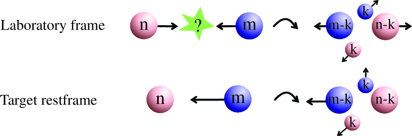
Figure 8.1: To implement the scattering of two pseudoparticles we transform to the rest frame of the target particle (shown as red/light gray) and computes the probability $P(n)$ that a single incident particle (shown as blue/dark gray) during a timestep $\Delta t$ is scattered on the $n$ target particles. If the incident particle has weight $m$, then $k=P(n)m$ particles will interact and two new pseudoparticles are created.

To increase effective spectral resolution we have instead decided to take a more direct approach. For simplicity we will here describe the method for a two-particle interaction, and disregard all factors converting code units to physical units. For example, the weight of a pseudoparticle is proportional to the number of physical particles in the pseudoparticle. Although, these prefactors all represent trivial conversions of units, they must be taken into account in the real code.

Consider a single cell containing a single pseudoparticle (red) with weight $w_{t}=n$ and a single pseudoparticle (purple) with weight $w_{i}=m$, where $n>m$ (see Fig. 8.1). We first select the red particle as the target, since $n>m$, and the purple as the incident particle. We then transform the four velocity of the incident particle to the rest frame of the target particle, and calculate the total cross section $\sigma_{t}$ of the interaction. Conceptually we consider the process as a single incident particle approaching a slab of the target particle. The number density of target particles in the slab can be calculated from the weight $w_{t}$ as $\rho_{t}=w_{t}/\Delta V$, where $\Delta V=\Delta x\Delta y\Delta z$ is the volume of a single cell. Given the number density the probability that a single incident particle is scattered per unit length is

$$P_{l}=\rho_{t}\sigma_{t}=\frac{w_{t}\sigma_{t}}{\Delta V}$$ (8.2)

During a time step $\Delta t$ the incident particle travels $\Delta l=v_{i}\Delta t$, and the probability that a single incident particle is scattered then becomes

$$P_{S} =1-\exp\left[-P_{l}\Delta l\right]$$

$$=1-\exp\left[-\frac{w_{t}\sigma_{t}v_{i}\Delta t}{\Delta V}\right]$$ (8.3)

The weight of the incident pseudoparticle is $w_{i}=m$. Pseudoparticles represent an ensemble of particles. Therefore $P_{S}$ is the fraction of incident particles that are scattered on the target. To model the process we create two new particles with weight $w_{new}=w_{i}P_{S}=k$. Given the detailed interaction, we can calculate the theoretical angular distribution of scattered particles in accordance with the differential scattering cross section. Drawing from this distribution we find the momentum and energy of the new scattered particles. The weights of the target and incident particles are decreased to $w_{t}=n-k$ and $w_{i}=m-k$ respectively (see Fig. 8.1).

Our method faithfully represents the actual physics even for small cross sections. However, if all the particles are allowed to interact, the number of particles in the box will increase at least proportionally to the total number of particles squared. This is potentially a computational run away. Normally we will have on the order of up to $100$ particles per species per cell, but to be computationally efficient we only calculate interactions for a subset of the particles in a cell. This subset is chosen at random according to an arbitrary distribution we are free to select. If the probability that two particles are selected for scattering in a given timestep is $Q$ then the travelling length $\Delta l$ simply has to be adjusted as $\Delta l/Q$. If this arbitrary distribution is chosen cleverly, the particles with the largest cross section are actually the ones selected most often for scattering, and everything ends up as a balanced manner: We only calculate the full cross section and scattering as often as needed, and the computational load that is given to a certain particle is proportional to the probability of that particle to scatter. We rely on the merging of particles as described above to avoid the copious production of pseudoparticles. Every time the number of pseudoparticles in a given cell crosses a threshold, pseudoparticles are merged and this way the computational load per cell is kept within a given range.

8.2.2 Neutron decay

Free neutrons not bound in a nucleus will decay with a half-life a little longer than ten minutes. The neutron decays into an electron and a proton and an electron antineutrino to satisfy lepton number conservation

$$n\to p+e^{-}+\bar{\nu}_{e}$$ (8.4)

The rest mass difference of the process (0.78 MeV) goes into kinetic energy of the proton, electron and neutrino. Let the neutron lifetime be $\tau$ in code units. If $\tau$ is comparable to or less than a typical timestep, then practically all neutrons decay in one iteration, and it is irrelevant to include them. If $\tau$ is much larger than the total runtime, the neutron can be considered a stable particle (unless the neutron density in the box is much larger than the proton– or electron density). If instead $\tau\simeq\alpha\Delta t$ where $\alpha\sim 100$, then we can select a fraction $f$ of the pseudoparticle neutrons in each cell and let them decay. This is done in an analogous manner to the generic scattering process described above in section 8.2.1. The weight of the selected neutron is decreased with a factor

$$\exp\left[-\frac{f\Delta t}{\gamma\tau}\right]\,,$$ (8.5)

where $\gamma$ is the Lorentz boost of the neutron pseudoparticle and $f$ is chosen to give reasonable values for the decrease in the weight. At the same time a pair of electron and proton pseudoparticles is created with the same weight. The generated particles share the excess mass of the process (where the neutrino is neglected for now, but could be included in the future). The momenta are selected to give an isotropic distribution in the rest frame of the decaying neutron.

8.2.3 Compton scattering

Here we briefly describe a specific physical scattering mechanism, which have already been implemented in the code, namely Compton scattering.

Compton scattering is the relativistic generalization of the classical Thompson scattering process, where a low energy photon scatters of on a free electron. In the rest frame of the electron, the photon changes direction and loses energy to the electron, which is set in motion. The cross section for Thompson scattering is Rybicki and Lightman (1979)

$$\sigma_{T}=\frac{8\pi}{3}r_{0}^{2}$$ (8.6)

where $r_{0}\equiv e^{2}/(mc^{2})$ is called the classical electron radius. The Thompson scattering approximation is valid as long as the photon energy is much lower than the electron rest mass $h\nu\ll m_{e}c^{2}$ and the scattering can be regarded as elastic. For photon energies comparable to, or larger than, the electron rest mass, recoil effects must be taken into account. Measured in the electron rest frame we define $\epsilon_{1}$ as the photon energy before the scattering, $\epsilon_{2}$ as the photon energy after the scattering and $\theta$ the photon scattering angle (8.2).

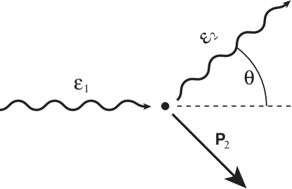
Figure 8.2: Schematic view of the Compton scattering process. Impinging on the electron, an incoming photon with energy $\epsilon_{1}$ is scattered into the angle $\theta$ with energy $\epsilon_{2}$. In the initial rest-frame of the electron, the electron will be recoiled to conserve energy and momentum.

By conservation of energy and momentum one can show (e.g. Rybicki and Lightman (1979)) that

$$\epsilon_{2}=\frac{\epsilon_{1}}{1+\frac{\epsilon_{1}}{m_{e}c^{2}}(1-\cos\theta)}$$ (8.7)

The differential cross section as a function of scattering angle is given by the Klein-Nishina formula Klein and Nishina (1929); Heitler (1954)

$$\frac{d\sigma_{C}}{d\Omega}=\frac{r_{0}^{2}}{2}\frac{\epsilon_{2}^{2}}{\epsilon_{1}^{2}}\left(\frac{\epsilon_{1}}{\epsilon_{2}}+\frac{\epsilon_{2}}{\epsilon_{1}}-\sin^{2}\theta\right)$$ (8.8)

The Klein-Nishina formula takes into account the relative intensity of scattered radiation, it incorporates the recoil factor, (or radiation pressure) and corrects for relativistic quantum mechanics. The total cross section is then

$$\sigma_{C}=\sigma_{T}\frac{3}{4}\left[\frac{1+x}{x^{3}}\left\{\frac{2x(1+x)}{1+2x}-\mathrm{ln}(1+2x)\right\}+\frac{1}{2x}\mathrm{ln}(1+2x)-\frac{1+3x}{(1+2x)^{2}}\right]$$ (8.9)

where $x\equiv h\nu/(mc^{2})$.

8.3 Preliminary results

To test the new code and it capabilities in regard to the inclusion of collisions, we have implemented and tested a simple scenario involving Compton scattering.

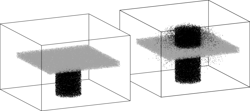
Figure 8.3: 3D scatter plot of a photon beam (black) passing through a cold pair plasma (gray). Left panel show initial setup where a photon beam is injected in the upward direction. Right panel shows how photons are scattered on the electron-positron pairs

In the test setup, we place a thin layer of cold electron-positron pair plasma in the computational box. From the boundary, we inject a monochromatic beam of photons all travelling perpendicular to the pair-layer (Fig. 8.3 left panel). As the beam passes through the plasma layer, photons are scattered (Fig. 8.3 left panel).

For each scattered photon we sample the weight of the photon and its direction (remembering that all particles are pseudoparticles that represent whole groups of particles). Fig. 8.4 shows the theoretical cross section as function of scattering angle compared with the result from the simulations. Four plots for different energies of the incoming photon beam are shown. We find excellent agreement between the simulation results and the theoretical predictions.

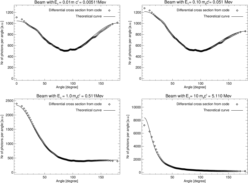
Figure 8.4: The theoretical Compton scattering differential cross section. We have performed a test experiment with an incoming laser beam on a very cold electron population. Over plotted the differential distribution is the theoretical curve according to Eqs. (8.8) and (8.7).

8.4 Discussion

A next generation PIC code that includes many different kinds of scattering process is under development. It will enable us to target problems that reside in the grey zone between the MHD and collisionless plasma domains. This domain covers many astrophysical scenarios of great interest counting internal shocks in gamma-ray bursts, solar flares and magnetic substorms, compact relativistic objects, supernova remnants and many more.

The concept of splitting/merging particles and keeping individual weights of each particle carry many important features. Variable weights represent the true statistics of a scattering process in an optimal way compared to the Monte Carlo approach. Also, for MPI-parallelization it is crucial that the number of particles per cell is kept more or less constant to ensure an optimal CPU load-balancing. To localize calculations we are employing a sorting algorithm that maintains neighbouring particles on the mesh as neighbours in memory. This is not only good for parallelization, but also makes all computations very cache efficient; a crucial requirement on modern computer architectures.

To test the infrastructure of the new code we have implemented Compton scattering as a simple scattering mechanism. The preliminary results are very promising in form of excellent agreement with the theoretical prediction. We note that a recent paper by Moderksi et al. (2005) provide an interesting test suite for various kind of particle-photon interactions that can be tested in the future. Merging particles has not been satisfactorily implemented yet. Parallelization of code is still not there yet, and is necessary to obtain the capability of performing truly large-scale experiments. In summary: Work has still to be done before we can start to investigate non-trivial astrophysical scenarios, nevertheless solid progress has already been made

This chapter has been written jointly by Christian Hededal and Troels Haugbølle, reflecting the fact that the development process of the next generation PIC code has been highly team based. Essentially everybody has contributed time and effort to every single source file of the code. It would not make sense to write the chapter separately, essentially repeating each other and reusing the same figures.

Chapter 9 Overall Discussion and Conclusions

The main source of information we have about gamma-ray bursts (GRBs) is from multi-wavelength observations of GRB afterglows. The radiation from GRB afterglows is generated in collisionless shocks between the external plasma (ISM) and the GRB jet. To make the right conclusions about burst parameters in these shocks, it is crucial that we have a firm understanding of how the radiation is generated. In the current working model, the radiation is believed to be emitted from power-law distributed electrons in a magnetic field. Following our lack of knowledge about the plasma-physical details, it is a general approach to parameterize this ignorance with the dimensionless parameters $\epsilon_{B}$, $\epsilon_{e}$ and $p$. As usual, $\epsilon_{B}$ and $\epsilon_{e}$ express the fraction of the total internal energy that is deposited in magnetic field and electrons and $p$ is the slope of the supposedly electron power-law momentum distribution function.

How the electrons are accelerated and what the origin and nature of the magnetic field in the afterglow shock is, remain open questions.

The main goal behind the work presented in this thesis has been to expand our knowledge about the microphysics of collisionless shocks. Attacking the problem from first principles, I have used particle-in-cell (PIC) simulations to investigate different aspects of these shocks. The results may be categorized into three groups: Magnetic fields in collisionless shocks, non-thermal electron acceleration and radiation from GRB afterglow shocks. I emphasize that these three components are highly interconnected and should be seen as pieces of the same puzzle.

9.1 Magnetic fields in collisionless shocks

Since the main focus is on GRB afterglows, I have investigated only electron-proton plasma shocks. The three-dimensional plasma PIC simulations illustrate from first principles a number of fundamental properties of collisionless plasma shocks.

• In unmagnetized or weakly magnetized relativistic shocks (below milligauss), the Weibel two-stream instability will unavoidably create a magnetic field that amounts to $\sim 10\%$ of the equipartition value ($\epsilon_{B}\sim 0.1$) but varies greatly through the shock.

• The nature of the magnetic field is predominantly transverse to the plasma flow, but a parallel magnetic component is also present. The parallel magnetic field strength is roughly $10\%$ of the transverse components. An electric field is also present with an energy density that amounts to roughly $10\%$ of the magnetic field energy density.

• The dominating instability is highly non-linear. The electrons are rapidly thermalized while the ions form current channels. These current channels are the main source of the magnetic field.

• Being Debye shielded by the hot electrons, the ion current channels are relatively stable and can penetrate deeply into the shock. Earlier thinking and concerns were that the generated magnetic field can only survive over an electron skin depth (Gruzinov, 2001). In the simulations presented here, the generated magnetic field is sustained for several hundred ion skin depths.

• The structure of the magnetic field is highly patched. The transverse coalescence scale is comparable to the ion skin depth. A spatial Fourier decomposition of the magnetic field shows that the structures follow a power-law distribution with negative slope.

• I find that in two-dimensional simulations of the Weibel two-stream instability, both the evolution of the plasma density profile and the generation of electromagnetic field are in agreement with three-dimensional simulations.

• With two-dimensional simulations, it has been able to capture a full relativistic, collisionless shock. The shock consists of three segments. 1) An upstream foreshock with great anisotropy, consisting of instreaming ISM plasma and upscattered shock particles. In this region, a strong magnetic field generation is taking place with $\epsilon_{B}=5-10\%$. 2) A dense thermalization region where the electrons and ions are close to equipartition ($\epsilon_{e}=50-80\%$). In this region, the magnetic field is relatively weak ($\epsilon_{B}\simeq 1\%$) but still strong enough to account for most GRB afterglow radiation estimates. 3) A hot downstream region where the magnetic field is of the order percents of equipartition. This region is clumpy, with large structures that are of the order $1-20$ ion skin depths in size.

• If the ejecta is already strongly magnetized with a transverse magnetic field (e.g. carried from the progenitor), the resulting dynamics is very complex: Particle deflection, charge separation and a mixture of the electromagnetic Weibel two-stream instability and the electrostatic Buneman instability make the resulting field very complicated with local reversal of the ambient field. Electrons are accelerated to a non-thermal distribution. In the case of strong parallel magnetic field, all instabilities are effectively damped.

• For an ambient magnetic field strength comparable to the ISM- field, the Weibel instability grows unhindered.

9.2 Non-thermal electron acceleration

There has been a general acceptance of Fermi acceleration as the mechanism that produces the desired electron distribution function. Nevertheless, this has never been proven in self-consistent numerical simulations. The idea of Fermi acceleration in collisionless shocks is currently facing several problems (see Chapter 1 for details):

• It is assumed that the particles scatter on electromagnetic waves, but the model does not self-consistently account for the generation of these waves nor for the back-reaction that the high-energy particle distribution has on the electromagnetic field.

• Relativistic Fermi acceleration requires the downstream magnetic field to be strongly turbulent on scales comparable to the gyro-resonant scale (e.g., Ostrowski and Bednarz 2002). This is in contrast with the standard synchrotron radiation scenario for GRB afterglows where it is assumed that the magnetic field is nearly constant on scales much larger than the gyro-radius (see however Medvedev (2000) and Chapter 7).

• Fermi acceleration requires pre-acceleration to above a certain threshold. How this pre-acceleration works and how large a fraction of the particles that participate in the non-thermal tail remains unexplained. In the most well studied mildly relativistic plasma shock (in the Crab nebula), observations are contradicting what is normally assumed about this threshold (Eichler and Waxman, 2005). Furthermore, Chandra images of the close by Supernova remnant SN 1006 fail to detect an x-ray halo in front of the shock, which is to be expected if the standard Fermi diffusive shock acceleration theory is correct. One expects an X-ray halo around the shock because higher energy electrons are expected to diffuse further ahead of the shock (Long et al., 2003).

I do not claim that Fermi acceleration cannot take place, but urge the need for a self-consistent treatment of the problem when computational resources allow this.

I have presented self-consistent, three-dimensional PIC simulations that have revealed a new non-thermal electron acceleration mechanism that differs substantially from Fermi acceleration. The acceleration is a natural consequence of the properties of relativistic collisionless shocks. Acceleration of electrons is directly related to the formation of ion current channels that are generated in the non-linear stage of the Weibel two-stream instability in the shock transition zone. This links particle acceleration closely together with magnetic field generation in collisionless shocks.

The resulting electron spectrum consists of a thermal component and a non-thermal component at high energies. This is in the line with arguments by Ryde (2005) and Rees and Meszaros (2004). In simulations of mildly relativistic shocks ($\Gamma=3$), the non-thermal component vanishes in the thermal pool. Computer experiment with a bulk flow with $\Gamma=15$ results in a power-law slope $p=2.7$ for the electron distribution function.

9.3 Radiation from GRB afterglow shocks

I have developed a tool that enables us to obtain radiation spectra directly from PIC simulations. The tool has been thoroughly tested and successfully reproduces spectra from synchrotron radiation, bremsstrahlung and undulator radiation from small-angle deflections. The tool has been used to investigate the properties of three-dimensional jitter radiation in magnetic fields with different turbulent configurations. By tracing ensembles of monoenergetic, isotropic distributions of electrons in a random magnetic field (whose power spectrum follows a power-law in the Fourier domain $P_{B}(k)\propto k^{\mu}$) I have computed and studied the resulting spectrum. I have focused on the weak field limit (where the deflection angle is less than the beaming cone angle, $K<1$). For all values of $\mu$, the radiation spectrum has a flat low-energy part (like bremsstrahlung). For $\mu<0$, the high-energy part of the spectrum follows a power-law with a slope $\alpha\simeq\mu-1$ independent of the electron energy. For $\mu>0$, the flat spectrum continues to higher frequencies than for $\mu<0$. The spectrum has a hard cut-off for high frequencies.

For all values of $\mu$ and $K<1$, the spectrum shifts in frequency with $\gamma^{2}$ and scales with the amplitude of the magnetic field squared $B^{2}$, in good agreement with Larmor’s formula for radiated power. In the limit of large deflections ($K>1$) the spectrum eventually converges through the wiggler spectrum to the ordinary synchrotron spectrum.

I have furthermore examined the radiation from electrons moving in 1) a magnetic field generated by the Weibel two-stream magnetic field and 2) a magnetic field that has the same average energy density and spectral power spectrum as the two-stream generated field. I find that even though the two spectra peak at the same frequency, there is a large difference above the peak-frequency. The reason is that in the magnetic field from the PIC simulations there exists a phase correlations resulting in higher magnetic peak values but smaller filling factor. The peak frequency of synchrotron/wiggler radiation scales linearly with the maximum magnetic field strength. Furthermore, from other PIC simulations we know that the high-energy electrons are found near the peaks in magnetic field.

In simulations of a collisionless shock that propagates with $\Gamma=15$ through the interstellar medium, the resulting radiation spectrum peaks around $10^{12}$Hz. Above this frequency, the spectrum follows a power-law $F\propto\nu^{-\beta}$, with $\beta=0.7$. Below the peak frequency, the spectrum follows a power law $F\propto\nu^{\alpha}$ with $\alpha\simeq 2/3$. This is steeper than the standard synchrotron value of $1/3$ and more compatible with observations. Both the slope and the peak is consistent with observations (e.g. Panaitescu 2001 who finds $\beta=0.67\pm 0.04$, a peak at $3\times 10^{11}$Hz and $\Gamma>10$ for the afterglow of GRB 000301c after five days).

I stress the following interesting point: If one hides all the real physical details of the magnetic field in the dimensionless parameters $\epsilon_{B}$, $\epsilon_{e}$, and $p$ the conclusion from standard synchrotron radiation theory would be that the slope of the electron distribution $N(\gamma)\propto\gamma^{-p}$ is found by solving $-\beta=-(p-1)/2=-0.70\ \to\ p=2.4$ (which is consistent with standard analysis of the GRB 000301c afterglow, Panaitescu 2001). This would appear to be consistent with Fermi acceleration and the supposedly universal $p\simeq 2.2\pm 0.2$: Case solved! But a closer look reveals that the acceleration mechanism is not Fermi acceleration. The electrons are instantaneously accelerated and decelerated in the highly complicated electric and magnetic field near the ion current channels. Strong radiation is produced in this process. The electron distribution behind the radiation is a mixture of a thermal component for low energies and a power-law component with $p=2.7$ for high energies (Hededal et al., 2004) (see also Chapter 6). The paths of the electrons are more random rather than circular and the electron distribution function varies with shock depth, as does the magnetic topology and strength. I repeat and emphasize that the electrons that produced the spectrum in Fig. 7.22 are not Fermi accelerated but a natural consequence of the Weibel two-stream instability.

9.4 Future work

In this thesis I have shown, from first prinicples, that from the collision of two plasma shells that are initially cold and non-magnetized, a strong small scale magnetic is generated ($\epsilon_{B}\sim 0.01-0.1$), particles are accelerated to non-thermal distributions and the emitted radiation is quite consistent with observations (comparing Fig. 7.22 and data from GRB 000301c, Panaitescu 2001). The next step is to determine the polarization in the synthetic spectra from the PIC simulations. Even though time did not allow this in this thesis, it will not be difficult with the tools that have already been developed. With the inclusion of polarization it will be possible to investigate how the radiation spectrum and polarization change as functions of the viewing angle relative to the jet propagation direction.

In the near future, computational resources will reach a level where one can resolve full three-dimensional collisionless shocks. This will enable us to make composite spectra from different simulations with bulk Lorentz factor varying with viewing angle, and in turn allow us to test many interesting aspects with regard to the jet structure and polarization predictions from shock-generated electromagnetic fields.

Finally, the new generation PIC code that is under development allows more of physics to be included in the simulations. Some of the main features are: High-energy photons are treated as particles, several scattering processes are included (e.g. Coulomb and Compton scattering), parallelization with MPI, pseudo particles with individual weights, etc. With this code it will become possible to study also the prompt GRB phase, where Compton scattering and pair processes are likely to be important.

Appendix A The Mean Free Path in a Blast Wave

In this appendix I make an estimate of the mean free path for Coulomb collisions of a relativistic electron with momentum $\gamma m_{e}\mbox{\boldmath$\mathrm{v}$}_{e}$ on ions in a plasma with density $n$.

First we examine the Coulomb collision between an electron and an ion. Without loss of generality, we may assume that the electron is travelling in the $yz$-plane along the $z$-axis and that an ion is positioned in $(x,y,z)=(0,-b,0)$. The ion is surrounded by an electric field. Because of Lorentz contraction and symmetry arguments we can assume that the electron will only be affected by the component that is transverse to $\mbox{\boldmath$\mathrm{v}$}_{e}$, namely $E_{y}$. In the reference frame of the electron, this component is given by (Rybicki and Lightman, 1979):

$$E_{y}=\frac{1}{4\pi\epsilon_{0}}\frac{q\gamma b}{(\gamma^{2}v_{e}^{2}t^{2}+b^{2})^{3/2}}.$$ (A.1)

Here $t$ is the time, centered so that the electron is in $(0,0,0)$ at $t=0$. The force felt by the electron is $\mbox{\boldmath$\mathrm{F}$}=qE_{y}\hat{\mbox{\boldmath$\mathrm{e}$}}_{y}$. The change in the electron’s momentum $\delta p$ is found as:

$$\delta p=\int F_{y}dt=\int qE_{y}dt=\frac{1}{4\pi\epsilon_{0}}\frac{q^{2}\gamma t}{b\sqrt{\gamma^{2}v_{e}^{2}t^{2}+b^{2}}}.$$ (A.2)

The pulse from the ion is felt by the electron in the short time interval $T\simeq b/(\gamma v_{v})$. Inserting this into Eq. A.2 we find

$$\delta p=\frac{1}{4\pi\epsilon_{0}}\frac{q^{2}}{\sqrt{2}v_{e}b}.$$ (A.3)

We are interested in collisions that alter the impinging electrons momentum significantly with $\delta p\simeq\gamma m_{e}v_{e}$, and we can thus find the distance $b_{c}$ for such a collision:

$$\delta p\simeq\gamma m_{e}v_{e}\ \ \ \ \Rightarrow$$

$$b_{c}\simeq\frac{1}{4\pi\epsilon_{0}}\frac{q^{2}}{\sqrt{2}\gamma m_{e}v_{e}^{2}}.$$ (A.4)

Thus, the cross section for the collision is

$$\sigma_{c}=\pi b_{c}^{2}=\frac{q^{4}}{16\pi\epsilon_{0}^{2}\sqrt{2}\gamma^{2}m_{e}^{2}v_{e}^{4}}.$$ (A.5)

The collision frequency is $\nu_{c}=n\sigma_{c}v_{e}$ and from this we find the mean free path for a full collision:

$$\lambda_{c}\equiv\frac{v_{e}}{\nu_{c}}=\frac{1}{n\sigma_{c}}=\frac{16\pi\epsilon_{0}^{2}\sqrt{2}\gamma^{2}m_{e}^{2}v_{e}^{4}}{nq^{4}}.$$ (A.6)

In reality, the mean free path somewhat shorter because of accumulation of small angle deflections. We can correct for this by introducing a correction factor $1/\ln\Lambda$, which is of the order of 0.1 (Spitzer, 1962).

For a electron in a blast wave that is expanding with Lorentz factor $\gamma\simeq\Gamma=10$, into an interstellar medium with density $n\simeq 10^{6}\mathrm{m}^{-3}$, the mean free path for a collision is larger than $10^{23}$m. Comparing this number with the typical size of a GRB blast wave $\sim 10^{14}$m we conclude that it is reasonable to neglect collisions between the ejecta and ISM, and that the shock between the two is to be regarded as a collisionless shock.

Appendix B Integration of $\frac{dP}{d\Omega}$

We wish to integrate Eq. 2.8 over all directions $\mathrm{n}$ through the solid angle $d\Omega$.

$$\frac{dP_{rad}}{d\Omega}=\frac{\mu_{0}q^{2}c}{16\pi^{2}}\frac{\left[\mbox{\boldmath$\mathrm{n}$}\times\left\{\left(\mbox{\boldmath$\mathrm{n}$}-\mbox{\boldmath$\mathrm{\beta}$}\right)\times\mbox{\boldmath$\dot{\mathrm{\beta}}$}\right\}\right]^{2}}{\left(1-\mbox{\boldmath$\mathrm{n\cdot\beta}$}\right)^{5}}.$$ (B.1)

Without loss of generalization we define a Cartesian coordinate system with the $x$-axis along the particles velocity vector $\mathrm{\beta}$ and the acceleration vector $\dot{\mathrm{\beta}}$ in the $x$-$y$ plane (Fig. B.1).

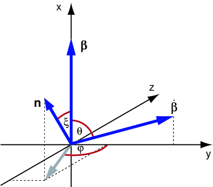
Figure B.1: We define a coordinate system with the $x$-axis along the velocity vector $\mathrm{\beta}$. For the integration over the unit solid angle $d\Omega$ around the unit vector we use the polar coordinates $(\xi,\varphi)$. The particle is accelerated at some angle $\theta$ to the velocity vector.

Integration over the unit solid angle $d\Omega$ then yields:

$$P_{rad}=\int\frac{dP_{rad}}{d\Omega}d\Omega=\int_{0}^{2\pi}\int_{0}^{\pi}\frac{dP_{rad}}{d\Omega}\sin\xi d\xi d\varphi.$$ (B.2)

With the definition of the polar angles in Fig. B.1 we can writte out $\mathrm{\beta}$, $\dot{\mathrm{\beta}}$ and $\mathrm{n}$:

$$\mbox{\boldmath$\mathrm{\beta}$}=\beta\left(\begin{array}[]{c}1\\ 0\\ 0\end{array}\right),\ \ \ \ \ \mbox{\boldmath$\dot{\mathrm{\beta}}$}=\dot{\beta}\left(\begin{array}[]{c}\cos\theta\\ \sin\theta\\ 0\end{array}\right),\ \ \ \ \ \mbox{\boldmath$\mathrm{n}$}=\left(\begin{array}[]{c}\cos\xi\\ \sin\xi\cos\varphi\\ \sin\xi\sin\varphi\end{array}\right)$$ (B.3)

$$\frac{dP_{rad}}{d\Omega}=\frac{\mu_{0}q^{2}c}{16\pi^{2}} \Big{\{}\left|\dot{\beta}\sin\xi\left[(\beta-\cos\xi)\cos\varphi\sin\theta+\cos\theta\sin\xi\right]\right|^{2}$$ (B.4)

$$+\left|\dot{\beta}\sin\xi(\cos\theta\cos\xi+\cos\varphi\sin\theta\sin\xi)\sin\varphi\right|^{2}$$

$$+\Big{|}\dot{\beta}\cos\xi((\beta-\cos\xi)\sin\theta+\cos\theta\cos\varphi\sin\xi)$$

$$-\dot{\beta}\sin\theta\sin^{2}\xi\sin^{2}\varphi\Big{|}^{2}\Big{\}}$$

$$/(1-|\beta|)^{5}.$$

Inserting Eq. B.4 into Eq. B.2 we perform the integration in two steps:

$$P_{rad} = \int_{0}^{2\pi}\int_{0}^{\pi}\frac{dP_{rad}}{d\Omega}\sin\xi d\xi d\varphi$$ (B.5)

$$= \int_{0}^{\pi}\dot{\beta}^{2}\pi\big{\{}(11+6\beta^{2}+2\beta^{2}\cos(2\xi)-2\cos(2\theta)$$

$$(1+3\beta^{2}+(3+\beta^{2})\cos(2\xi))-32\beta\cos\xi\sin^{2}\theta)$$

$$\sin\xi-\sin(3\xi)\big{\}}/(16(1-\beta\cos\xi)^{5})\sin\xi d\xi$$

$$= \frac{\mu_{0}q^{2}c}{12\pi}\gamma^{6}\dot{\beta}^{2}\left(2-\beta^{2}(1-\cos(2\theta)\right)$$

$$= \frac{\mu_{0}q^{2}c}{6\pi}\gamma^{6}\dot{\beta}^{2}\left(1-\beta^{2}\sin^{2}\theta\right).$$

Appendix C Spectral distribution of Synchrotron Radiation

Here we derive the spectral distribution of synchrotron radiation. We follow the standard derivation found in many textbooks (e.g. Rybicki and Lightman (1979)), but keep the full angular dependency. We start with the expression for the radiated energy pr. unit frequency pr. unit solid angle (Eq. 7.8)

$$\frac{d^{2}W}{d\omega d\Omega}=\frac{q^{2}}{16\pi^{3}\epsilon_{0}c}\left|\int_{-\infty}^{\infty}{\frac{\mbox{\boldmath$\mathrm{n}$}\times[(\mbox{\boldmath$\mathrm{n}$}-\mbox{\boldmath$\mathrm{\beta}$})\times\mbox{\boldmath$\dot{\mathrm{\beta}}$}]}{(1-\mbox{\boldmath$\mathrm{\beta\cdot n}$})^{2}}\ e^{i\omega(t^{\prime}-\mbox{\boldmath$\mathrm{n\cdot r}$}(t^{\prime})/c)}dt^{\prime}}\right|^{2}.$$ (C.1)

Integration by parts and using the relation

$$\frac{\mbox{\boldmath$\mathrm{n}$}\times[(\mbox{\boldmath$\mathrm{n}$}-\mbox{\boldmath$\mathrm{\beta}$})\times\mbox{\boldmath$\dot{\mathrm{\beta}}$}]}{(1-\mbox{\boldmath$\mathrm{\beta\cdot n}$})^{2}}=\frac{d}{dt}\left[\frac{\mbox{\boldmath$\mathrm{n}$}\times(\mbox{\boldmath$\mathrm{n}$}\times\mbox{\boldmath$\mathrm{\beta}$})}{1-\mbox{\boldmath$\mathrm{\beta\cdot n}$}}\right],$$ (C.2)

we can rewrite into the expression

$$\frac{d^{2}W}{d\omega d\Omega}=\frac{q^{2}\omega^{2}}{16\pi^{3}\epsilon_{0}c}\left|\int_{-\infty}^{\infty}\mbox{\boldmath$\mathrm{n}$}\times(\mbox{\boldmath$\mathrm{n}$}\times\mbox{\boldmath$\mathrm{\beta}$})e^{i\omega(t^{\prime}-\mbox{\boldmath$\mathrm{n\cdot r}$}(t^{\prime})/c)}dt\right|^{2}.$$ (C.3)

We now expand the terms in the integrand

$$t^{\prime}-\mbox{\boldmath$\mathrm{n\cdot r}$}(t^{\prime})/c) = t^{\prime}-\frac{r_{L}}{c}\cos\theta\sin(\beta ct^{\prime}/a)$$ (C.4)

$$\simeq (1-\beta\cos\theta)t^{\prime}+\frac{\beta^{3}c^{2}\cos\theta}{6r_{L}^{2}}{t^{\prime}}^{3}$$

$$= \frac{1}{2}\left(\theta_{\beta}^{2}t^{\prime}+\frac{\beta^{3}c^{2}\cos\theta}{3r_{L}^{2}}{t^{\prime}}^{3}\right),$$

where $\theta_{\beta}^{2}\equiv 2(1-\beta\cos\theta)$.

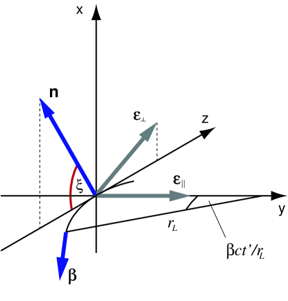
Figure C.1: We define a coordinate system with the $x$-axis along the velocity vector $\mathrm{\beta}$. For the integration over the unit solid angle $d\Omega$ around the unit vector we use the polar coordinates $(\theta,\varphi)$. The particle is accelerated at some angle $\theta$ to the velocity vector.

$$\mbox{\boldmath$\mathrm{n}$}\times(\mbox{\boldmath$\mathrm{n}$}\times\mbox{\boldmath$\mathrm{\beta}$}) = \beta\left[\sin\theta\cos(\beta ct^{\prime}/r_{L})\mbox{\boldmath$\mathrm{\epsilon}$}_{\perp}-\sin(\beta ct^{\prime}/r_{L})\mbox{\boldmath$\mathrm{\epsilon}$}_{\parallel}\right]$$ (C.5)

$$\simeq \beta\sin\theta\mbox{\boldmath$\mathrm{\epsilon}$}_{\perp}-\beta^{2}ct^{\prime}/r_{L}\mbox{\boldmath$\mathrm{\epsilon}$}_{\parallel}$$

The radiation has to polarization components

$$\frac{d^{2}W}{d\omega d\Omega}=\frac{d^{2}W_{\perp}}{d\omega d\Omega}+\frac{d^{2}W_{\parallel}}{d\omega d\Omega}$$ (C.6)

$$\frac{d^{2}W_{\perp}}{d\omega d\Omega} = \frac{q^{2}\omega^{2}}{16\pi^{3}\epsilon_{0}c}\left|\int_{-\infty}^{\infty}\beta\sin\theta\exp\left[\frac{i\omega}{2}(\theta_{\beta}^{2}t^{\prime}+\frac{\beta^{3}c^{2}\cos\theta}{3r_{L}^{2}}{t^{\prime}}^{3})\right]dt^{\prime}\right|^{2}$$ (C.7)

$$\frac{d^{2}W_{\parallel}}{d\omega d\Omega} = \frac{q^{2}\omega^{2}}{16\pi^{3}\epsilon_{0}c}\left|\int_{-\infty}^{\infty}\frac{\beta^{2}ct^{\prime}}{a}\exp\left[\frac{i\omega}{2}(\theta_{\beta}^{2}t^{\prime}+\frac{\beta^{3}c^{2}\cos\theta}{3r_{L}^{2}}{t^{\prime}}^{3})\right]dt^{\prime}\right|^{2}.$$ (C.8)

We now define

$$K=\frac{q^{2}\omega^{2}}{16\pi^{3}\epsilon_{0}c}\ ,\ \ \ \chi\equiv\frac{\omega r_{L}\theta_{\beta}^{3}}{3c}\ ,\ \ \ y\equiv\frac{ct^{\prime}}{r_{L}\theta_{\beta}}$$ (C.9)

$$\frac{d^{2}W_{\perp}}{d\omega d\Omega} = K\sin^{2}\theta\left(\frac{r_{L}\theta_{\beta}}{c}\right)^{2}\left|\int_{-\infty}^{\infty}\exp\left[\frac{3}{2}i\chi(y+\frac{1}{3}\cos\theta\beta^{3}y^{3})\right]dy\right|^{2}$$ (C.10)

$$\frac{d^{2}W_{\parallel}}{d\omega d\Omega} = K\left(\frac{r_{L}\theta_{\beta}^{2}\beta^{2}}{c}\right)^{2}\left|\int_{-\infty}^{\infty}y\exp\left[\frac{3}{2}i\chi(y+\frac{1}{3}\cos\theta\beta^{3}y^{3})\right]dy\right|^{2}.$$ (C.11)

We now focus solely on the integrals. We hide all the coefficients by introducing the variables $x$ and $z$.

$$x\equiv\frac{3}{2}\chi\ ,\ \ \ a\equiv\frac{1}{2}\cos\theta\beta^{3}\chi.$$ (C.12)

First, we expand the exponential functions in a geometric representation,

$$\exp\left[i(xy+ay^{3})\right] = \cos(xy+ay^{3})+i\sin(xy+ay^{3}).$$ (C.13)

The solutions to the integrals of Eq. C.10 and Eq. C.11 are expressed by Abramowitz and Stegun (1964):

$$\int_{-\infty}^{\infty}\exp\left[i(xy+ay^{3})\right]dy = \int_{-\infty}^{\infty}\cos(xy+ay^{3})dy$$ (C.14)

$$= 2(3a)^{-1/3}\pi\mathrm{Ai}\left[(3a)^{-1/3}x\right]$$

$$\int_{-\infty}^{\infty}y\exp\left[i(xy+ay^{3})\right]dy = \int_{-\infty}^{\infty}y\sin(xy+ay^{3})dy$$

$$\frac{d}{dx}\int_{-\infty}^{\infty}\cos(xy+ay^{3})dy = 2(3a)^{-2/3}\pi\mathrm{Ai}^{\prime}\left[(3a)^{-1/3}x\right],$$ (C.15)

where $\mathrm{Ai}(z)$ is the Airy function. The Airy function and its derivative can be expressed in terms of the modified Bessel function of the second kind:

$$K_{\frac{1}{3}}(\zeta) = \pi\sqrt{\frac{3}{z}}\mathrm{Ai}(z)$$ (C.16)

$$K_{\frac{2}{3}}(\zeta) = -\pi\frac{\sqrt{3}}{z}\mathrm{Ai}^{\prime}(z),$$ (C.17)

where $z\equiv(\tfrac{3}{2}\zeta)^{2/3}$. I our case, $z=(3a)^{-1/3}x$ and by comparing these two expressions for $z$ and reinstating the definitions of $a$ and $x$ we find the relation:

$$\zeta=\frac{\chi}{\sqrt{\cos\theta\beta^{3}}}.$$ (C.18)

Thus, the Airy function and its derivative in Eq. C.14 and Eq. C.15 can be replaced with:

$$\mathrm{Ai}\left[(3a)^{-1/3}x\right] = K_{\frac{1}{3}}\left(\chi/\sqrt{\cos\theta\beta^{3}}\right)\sqrt{\frac{z}{3\pi^{2}}}$$ (C.19)

$$\mathrm{Ai}^{\prime}\left[(3a)^{-1/3}x\right] = -K_{\frac{2}{3}}\left(\chi/\sqrt{\cos\theta\beta^{3}}\right)\frac{z}{\sqrt{3\pi^{2}}}$$ (C.20)

with $z=(3a)^{-1/3}x$. With these expressions we arrive at the final result of Eq. C.10 and Eq. C.11:

$$\frac{d^{2}W_{\perp}}{d\omega d\Omega} = \frac{q^{2}\omega^{2}}{12\pi^{3}\epsilon_{0}c}\left(\frac{r_{L}\theta_{\beta}\sin\theta}{c}\right)^{2}\frac{\left|K_{\frac{1}{3}}\left(\chi/\sqrt{\cos\theta\beta^{3}}\right)\right|^{2}}{(\cos\theta\beta^{3})}$$ (C.21)

$$\frac{d^{2}W_{\parallel}}{d\omega d\Omega} = \frac{q^{2}\omega^{2}}{12\pi^{3}\epsilon_{0}c}\left(\frac{r_{L}\theta_{\beta}^{2}\beta^{2}}{c}\right)^{2}\frac{\left|K_{\frac{2}{3}}\left(\chi/\sqrt{\cos\theta\beta^{3}}\right)\right|^{2}}{(\cos\theta\beta^{3})^{2}}$$ (C.22)

References

- Abramowitz and Stegun (1964) Abramowitz, M. and Stegun, I. A.: 1964, Handbook of Mathematical Functions
- Achterberg et al. (2001) Achterberg, A., Gallant, Y. A., Kirk, J. G., and Guthmann, A. W.: 2001, MNRAS 328, 393
- Amati et al. (2002) Amati, L., Frontera, F., Tavani, M., in’t Zand, J. J. M., Antonelli, A., Costa, E., Feroci, M., Guidorzi, C., Heise, J., Masetti, N., Montanari, E., Nicastro, L., Palazzi, E., Pian, E., Piro, L., and Soffitta, P.: 2002, A&A 390, 81
- Attwood (2000) Attwood: 2000, Sof x-rays and extreme ultraviolet radiation : principles and applications, Cambridge University Press, New York, 1st edition
- Attwood et al. (1993) Attwood, D., Sommargren, G., Beguiristain, R., Nguyen, K., Bokor, J., Ceglio, N., Jackson, K., Koike, M., and Underwood, J.: 1993, Appl. Opt. 32, 7022
- Axford et al. (1977) Axford, W. I., Leer, E., and Skadron, G.: 1977, Proc. 15th Int. Cosmic-Ray Conf. (Plovdiv 11, 132
- Balbus (2003) Balbus, S. A.: 2003, ARAA 41, 555
- Band et al. (1993) Band, D., Matteson, J., Ford, L., Schaefer, B., Palmer, D., Teegarden, B., Cline, T., Briggs, M., Paciesas, W., Pendleton, G., Fishman, G., Kouveliotou, C., Meegan, C., Wilson, R., and Lestrade, P.: 1993, ApJ 413, 281
- Baring (2005) Baring, M. G.: 2005, ArXiv Astrophysics e-prints - astro-ph/0502156
- Baring and Braby (2004) Baring, M. G. and Braby, M. L.: 2004, ApJ 613, 460
- Bednarz and Ostrowski (1998) Bednarz, J. and Ostrowski, M.: 1998, Physical Review Letters 80, 3911
- Bell (1978) Bell, A. R.: 1978, MNRAS 182, 147
- Beloborodov (2002) Beloborodov, A. M.: 2002, ApJ 565, 808
- Berger et al. (2003) Berger, E., Kulkarni, S. R., and Frail, D. A.: 2003, ApJ 590, 379
- Birdsall and Langdon (1991) Birdsall, C. and Langdon, B.: 1991, Plasma Physics via Computer Simulations, Adam Hilger, New York & Philadelphia
- Blandford and McKee (1976) Blandford, R. D. and McKee, C. F.: 1976, Physics of Fluids 19, 1130
- Blandford and Ostriker (1978) Blandford, R. D. and Ostriker, J. P.: 1978, ApJL 221, L29
- Bloom et al. (2001) Bloom, J. S., Djorgovski, S. G., and Kulkarni, S. R.: 2001, ApJ 554, 678
- Bloom et al. (2003) Bloom, J. S., Frail, D. A., and Kulkarni, S. R.: 2003, ApJ 594, 674
- Børve et al. (2001) Børve, S., Omang, M., and Trulsen, J.: 2001, ApJ 561, 82
- Buneman (1958) Buneman, O.: 1958, Phys. Rev. Lett. 1, 8
- Buneman (1959) Buneman, O.: 1959, Phys. Rev. 115, 503
- Buneman et al. (1992) Buneman, O., Neubert, T., and Nishikawa, K.: 1992, IEEE Transactions on Plasma Science 20, 810
- Califano (2002) Califano, F., C. T. C. C.: 2002, Phys. Plasmas 9, 451
- Califano et al. (1998) Califano, F., S., P., Bulanov, V., and Mangeney, A.: 1998, Phys. Rev. E 57, 7048
- Campana et al. (2005) Campana, S., Antonelli, L. A., Chincarini, G., Covino, S., Cusumano, G., Malesani, D., Mangano, V., Moretti, A., Pagani, C., Romano, P., Tagliaferri, G., Capalbi, M., Perri, M., Giommi, P., Angelini, L., Boyd, P., Burrows, D. N., Hill, J. E., Gronwall, C., Kennea, J. A., Kobayashi, S., Kumar, P., Meszaros, P., Nousek, J. A., Roming, P. W. A., Zhang, B., Abbey, A. F., Beardmore, A. P., Breeveld, A., Goad, M. R., Godet, O., Mason, K. O., Osborne, J. P., Page, K. L., Poole, T., and Gehrels, N.: 2005, Accepted for publication, ApJ - (astro-ph/0504331)
- Costa (1997) Costa, E. e. a.: 1997, Nature 387
- Dawson et al. (1983) Dawson, J. M., Decyk, V. K., Huff, R. W., Jechart, I., Katsouleas, T., Leboeuf, J. N., Lembege, B., Martinez, R. M., Ohsawa, Y., and Ratliff, S. T.: 1983, Physical Review Letters 50, 1455
- Dieckmann et al. (2000) Dieckmann, M. E., Chapman, S. C., McClements, K. G., Dendy, R. O., and Drury, L. O.: 2000, A&A 356, 377
- Dieckmann et al. (2004) Dieckmann, M. E., Eliasson, B., and Shukla, P. K.: 2004, ApJ 617, 1361
- Draine and McKee (1993) Draine, B. T. and McKee, C. F.: 1993, ARA&A 31, 373
- Eichler and Waxman (2005) Eichler, D. and Waxman, E.: 2005, ArXiv Astrophysics e-prints - astro-ph/0502070
- Fender et al. (2004) Fender, R., Wu, K., Johnston, H., Tzioumis, T., Jonker, P., Spencer, R., and van der Klis, M.: 2004, Nature 427, 222
- Fermi (1949) Fermi, E.: 1949, Physical Review 75, 1169
- Fishman and Meegan (1995) Fishman, G. J. and Meegan, C. A.: 1995, Annu. Rev. Astron. Astrophys. 33, 415
- Frail et al. (2001) Frail, D. A., Kulkarni, S. R., Sari, R., Djorgovski, S. G., Bloom, J. S., Galama, T. J., Reichart, D. E., Berger, E., Harrison, F. A., Price, P. A., Yost, S. A., Diercks, A., Goodrich, R. W., and Chaffee, F.: 2001, ApJL 562, L55
- Frederiksen (2002) Frederiksen, J. T.: 2002, Relativistic Collisionless Plasma Simulations, Master thesis
- Frederiksen et al. (2002) Frederiksen, J. T., Hededal, C. B., Haugbølle, T., and Nordlund, Å.: 2002, in Beaming and Jets in Gamma Ray Bursts, pp 115–+
- Frederiksen et al. (2004) Frederiksen, J. T., Hededal, C. B., Haugbølle, T., and Nordlund, Å.: 2004, ApJL 608, L13
- Freid (1959) Freid, B. D.: 1959, Phys. Fluids 2, 337
- Galama et al. (1998) Galama, T. J., Vreeswijk, P. M., van Paradijs, J., Kouveliotou, C., Augusteijn, T., Bohnhardt, H., Brewer, J. P., Doublier, V., Gonzalez, J.-F., Leibundgut, B., , and coauthors, .: 1998, Nature 395, 670
- Galeev A.A. (1995) Galeev A.A., Malkov M.A., V. H.: 1995, J. Plasma Phys. 54, 59
- Ghirlanda et al. (2004) Ghirlanda, G., Ghisellini, G., and Lazzati, D.: 2004, ApJ 616, 331
- Goodman (1986) Goodman, J.: 1986, ApJL 308, L47
- Goodman (1997) Goodman, J.: 1997, New Astronomy 2, 449
- Governato et al. (2004) Governato, F., Mayer, L., Wadsley, J., Gardner, J. P., Willman, B., Hayashi, E., Quinn, T., Stadel, J., and Lake, G.: 2004, ApJ 607, 688
- Granot and Sari (2002) Granot, J. and Sari, R.: 2002, ApJ 568, 820
- Gruzinov (1999) Gruzinov, A.: 1999, ApJL 525, L29
- Gruzinov (2001) Gruzinov, A.: 2001, ApJL 563, L15
- Gruzinov and Waxman (1999) Gruzinov, A. and Waxman, E.: 1999, ApJ 511, 852
- Harrison et al. (1999) Harrison, F. A., Bloom, J. S., Frail, D. A., Sari, R., Kulkarni, S. R., Djorgovski, S. G., Axelrod, T., Mould, J., Schmidt, B. P., Wieringa, M. H., Wark, R. M., Subrahmanyan, R., McConnell, D., McCarthy, P. J., Schaefer, B. E., McMahon, R. G., Markze, R. O., Firth, E., Soffitta, P., and Amati, L.: 1999, 523, L121
- Heavens and Drury (1988) Heavens, A. F. and Drury, L. O.: 1988, MNRAS 235, 997
- Hededal et al. (2004) Hededal, C. B., Haugbølle, T., Frederiksen, J. T., and Nordlund, Å.: 2004, ApJL 617, L107
- Hededal and Nishikawa (2005) Hededal, C. B. and Nishikawa, K.: 2005, ApJL 623, L89
- Heitler (1954) Heitler, W.: 1954, The Quantum Theory of Radiation, Oxford Clarendom Press, Exford, 3rd edition
- Hesse et al. (2001) Hesse, M., Birn, J., and Kuznetsova, M.: 2001, JGR 106, 3721
- Hesse et al. (1999) Hesse, M., Schindler, K., Birn, J., and Kuznetsova, M.: 1999, Phys. Plasmas 8, 1781
- Hjorth et al. (2003) Hjorth, J., Sollerman, J., Møller, P., Fynbo, J. P. U., Woosley, S. E., Kouveliotou, C., Tanvir, N. R., Greiner, J., Andersen, M. I., Castro-Tirado, A. J., Castro Cerón, J. M., Fruchter, A. S., Gorosabel, J., Jakobsson, P., Kaper, L., Klose, S., Masetti, N., Pedersen, H., Pedersen, K., Pian, E., Palazzi, E., Rhoads, J. E., Rol, E., van den Heuvel, E. P. J., Vreeswijk, P. M., Watson, D., and Wijers, R. A. M. J.: 2003, Nature 423, 847
- Hoshino et al. (1992) Hoshino, M., Arons, J., Gallant, Y. A., and Langdon, A. B.: 1992, ApJ 390, 454
- Hoshino and Shimada (2002) Hoshino, M. and Shimada, N.: 2002, ApJ 572, 880
- Jackson (1999) Jackson, J. D.: 1999, Classical Electrodynamics, John Wiley & Sons, Inc, New York, 3rd edition
- Katsouleas and Dawson (1983) Katsouleas, T. and Dawson, J. M.: 1983, Physical Review Letters 51, 392
- Katz (1994) Katz, J. I.: 1994, ApJL 432, L107
- Kazimura et al. (1998) Kazimura, Y., Sakai, J. I., Neubert, T., and Bulanov, S. V.: 1998, ApJL 498, L18
- Kincaid (1977) Kincaid, B. M.: 1977, J. Appl. Phys 48, 2684
- Kirk et al. (2000) Kirk, J. G., Guthmann, A. W., Gallant, Y. A., and Achterberg, A.: 2000, ApJ 542, 235
- Kirk and Schneider (1987) Kirk, J. G. and Schneider, P.: 1987, ApJ 315, 425
- Klebesadel et al. (1973) Klebesadel, R., Strong, I., and Olson, R.: 1973, ApJ 182
- Klein and Nishina (1929) Klein, O. and Nishina, Y.: 1929, Zeits. für Physics 52, 853
- Kulkarni et al. (1999) Kulkarni, S. R., Djorgovski, S. G., Odewahn, S. C., Bloom, J. S., Gal, R. R., Koresko, C. D., Harrison, F. A., Lubin, L. M., Armus, L., Sari, R., and coauthors, .: 1999, Nature 398, 389
- Kulkarni et al. (1998) Kulkarni, S. R., Frail, D. A., Wieringa, M. H., Ekers, R. D., Sadler, E. M., Wark, R. M., Higdon, J. L., Phinney, E. S., and Bloom, J. S.: 1998, Nature 395, 663
- Kumar (2000) Kumar, P.: 2000, ApJL 538, L125
- Lamb (1995) Lamb, D. Q.: 1995, PASP 107, 1152
- Landau and Lifshitz (1975) Landau, L. D. and Lifshitz, E. M.: 1975, The Classical Theory of Fields, Vol. 2 of Course In Theoretical Physics, Butterworth-Heinemann, 4th edition
- Lazzati et al. (2004) Lazzati, D., Covino, S., Gorosabel, J., Rossi, E., Ghisellini, G., Rol, E., Castro Cerón, J. M., Castro-Tirado, A. J., Della Valle, M., di Serego Alighieri, S., Fruchter, A. S., Fynbo, J. P. U., Goldoni, P., Hjorth, J., Israel, G. L., Kaper, L., Kawai, N., Le Floc’h, E., Malesani, D., Masetti, N., Mazzali, P., Mirabel, F., Moller, P., Ortolani, S., Palazzi, E., Pian, E., Rhoads, J., Ricker, G., Salmonson, J. D., Stella, L., Tagliaferri, G., Tanvir, N., van den Heuvel, E., Wijers, R. A. M. J., and Zerbi, F. M.: 2004, A&A 422, 121
- Lee et al. (2004) Lee, R. E., Chapman, S. C., and Dendy, R. O.: 2004, ApJ 604, 187
- Lembege et al. (2004) Lembege, B., Giacalone, J., Scholer, M., Hada, T., Hoshino, M., Krasnoselskikh, V., Kucharek, H., Savoini, P., and Terasawa, T.: 2004, Space Science Reviews 110, 161
- Lipunov et al. (2001) Lipunov, V. M., Postnov, K. A., and Prokhorov, M. E.: 2001, Astronomy Reports 45, 236
- Long et al. (2003) Long, K. S., Reynolds, S. P., Raymond, J. C., Winkler, P. F., Dyer, K. K., and Petre, R.: 2003, ApJ 586, 1162
- Mészáros (2001) Mészáros, P.: 2001, Science 291, 79
- Mészáros (2002) Mészáros, P.: 2002, ARAA 40, 137
- Medvedev (2000) Medvedev, M. V.: 2000, ApJ 540, 704
- Medvedev (2005) Medvedev, M. V.: 2005, ArXiv Astrophysics e-prints - astro-ph/0503463
- Medvedev et al. (2005) Medvedev, M. V., Fiore, M., Fonseca, R. A., Silva, L. O., and Mori, W. B.: 2005, ApJL 618, L75
- Medvedev and Loeb (1999) Medvedev, M. V. and Loeb, A. .: 1999, ApJ 526, 697
- Meegan et al. (1992) Meegan, C. A., Fishman, G. J., Wilson, R. B., Horack, J. M., Brock, M. N., Paciesas, W. S., Pendleton, G. N., and Kouveliotou, C.: 1992, Nature 355, 143
- Meszaros and Rees (1993) Meszaros, P. and Rees, M. J.: 1993, ApJL 418, L59
- Moderksi et al. (2005) Moderksi, R., Sikora, M., Coppi, P. S., and Aharonian, F. A.: 2005, ArXiv Astrophysics e-prints - astro-ph/0504388
- Niemiec and Ostrowski (2004) Niemiec, J. and Ostrowski, M.: 2004, ApJ 610, 851
- Nishikawa et al. (2003) Nishikawa, K.-I., Hardee, P., Richardson, G., Preece, R., Sol, H., and Fishman, G. J.: 2003, ApJ 595, 555
- Nishikawa et al. (2005) Nishikawa, K.-I., Hardee, P., Richardson, G., Preece, R., Sol, H., and Fishman, G. J.: 2005, ApJ 622, 927
- Noguchi et al. (2004) Noguchi, K., Liang, E., and Nishimura, K.: 2004, ArXiv Astrophysics e-prints - astro-ph/0412310
- Ostrowski and Bednarz (2002) Ostrowski, M. and Bednarz, J.: 2002, A&A 394, 1141
- Paczynski (1986) Paczynski, B.: 1986, ApJL 308, L43
- Paczyński (1995) Paczyński, B.: 1995, PASP 107, 1167
- Paczyński and Rhoads (1993) Paczyński, B. and Rhoads, J. E.: 1993, ApJ 418, L5
- Paczyński and Xu (1994) Paczyński, B. and Xu, G.: 1994, ApJ 427, 708
- Panaitescu (2001) Panaitescu, A.: 2001, ApJ 556, 1002
- Panaitescu and Kumar (2001) Panaitescu, A. and Kumar, P.: 2001, ApJL 560, L49
- Panaitescu and Kumar (2002) Panaitescu, A. and Kumar, P.: 2002, ApJ 571, 779
- Panaitescu and Mészáros (1999) Panaitescu, A. and Mészáros, P.: 1999, ApJ 526, 707
- Piran (1996) Piran, T.: 1996, General Relativity and Gravitation 28, 1421
- Piran (1999) Piran, T.: 1999, Phys. Rep. 314, 575
- Piran (2005a) Piran, T.: 2005a, ArXiv Astrophysics e-prints - astro-ph/0503060
- Piran (2005b) Piran, T.: 2005b, Rev. Mod. Phys. 76, 1143
- Preece et al. (1998) Preece, R. D., Briggs, M. S., Mallozzi, R. S., Pendleton, G. N., Paciesas, W. S., and Band, D. L.: 1998, ApJL 506, L23
- Press et al. (1986) Press, W. H., Teukolsky, S. A., Vetterling, W. T., and Flannery, B. P.: 1986, Numerical Recipes in Fortran 77, Cambridge University Press, New York, 2nd edition
- Rees and Meszaros (1992) Rees, M. J. and Meszaros, P.: 1992, MNRAS 258, 41P
- Rees and Meszaros (1994) Rees, M. J. and Meszaros, P.: 1994, ApjL 430, L93
- Rees and Meszaros (2004) Rees, M. J. and Meszaros, P.: 2004, ArXiv Astrophysics e-prints - arXiv:astro-ph/0412702
- Rhoads (1997) Rhoads, J. E.: 1997, ApJL 487, L1
- Rhoads (1999) Rhoads, J. E.: 1999, ApJ 525, 737
- Rossi et al. (2002) Rossi, E., Lazzati, D., and Rees, M. J.: 2002, MNRAS 332, 945
- Rossi and Rees (2003) Rossi, E. and Rees, M. J.: 2003, MNRAS 339, 881
- Ruderman (1975) Ruderman, M.: 1975, New York Academy Sciences Annals 262, 164
- Rybicki and Lightman (1979) Rybicki, G. B. and Lightman, A. P.: 1979, Radiative Processes in Astrophysics, John Wiley & Sons, Inc, New York, 3rd edition
- Ryde (2005) Ryde, F.: 2005, ApJ Letters Accepted - astro-ph/0504450
- Sagdeev (1966) Sagdeev, R. Z.: 1966, Rev. Plasma Phys. 4, 23
- Sahu (1997) Sahu, K. C.: 1997, Bulletin of the American Astronomical Society 29, 1401
- Saito and Sakai (2003) Saito, S. and Sakai, J.: 2003, Phys. Plasma 11, 859
- Sakai and Matsuo (2004) Sakai, J.-I. and Matsuo, A.: 2004, Phys. Plasmas 11, 3251
- Sari and Piran (1995) Sari, R. and Piran, T.: 1995, ApJL 455, L143
- Sari et al. (1999) Sari, R., Piran, T., and Halpern, J. P.: 1999, ApJL 519, L17
- Sari et al. (1998) Sari, R., Piran, T., and Narayan, R.: 1998, ApJL 497, L17
- Schmitz et al. (2002) Schmitz, H., Chapman, S. C., and Dendy, R. O.: 2002, ApJ 579, 327
- Shemi and Piran (1990) Shemi, A. and Piran, T.: 1990, ApJL 365, L55
- Shimada and Hoshino (2004) Shimada, N. and Hoshino, M.: 2004, Phys. Plasmas 11, 1840
- Silva et al. (2003) Silva, L. O., Fonseca, A., R., Tonge, W., J., Dawson, and and, J. M.: 2003, ApJ 596
- Spitzer (1962) Spitzer, Jr., L.: 1962, Physics of Fully Ionized Gases, Interscience, New York, 2nd edition
- Stanek et al. (2005) Stanek, K. Z., Garnavich, P. M., Nutzman, P. A., Hartman, J. D., Garg, A., Adelberger, K., Berlind, P., Bonanos, A. Z., Calkins, M. L., Challis, P., Gaudi, B. S., Holman, M. J., Kirshner, R. P., McLeod, B. A., Osip, D., Reiprich, T. P. T. H., Romanishin, W., Spahr, T., Tegler, S. C., and Zhao, X.: 2005, ArXiv Astrophysics e-prints - astro-ph/0502319
- Stanek et al. (2003) Stanek, K. Z., Matheson, T., Garnavich, P. M., Martini, P., Berlind, P., Caldwell, N., Challis, P., Brown, W. R., Schild, R., Krisciunas, K., Calkins, M. L., Lee, J. C., Hathi, N., Jansen, R. A., Windhorst, R., Echevarria, L., Eisenstein, D. J., Pindor, B., Olszewski, E. W., Harding, P., Holland, S. T., and Bersier, D.: 2003, ApJL 591, L17
- Stern (2003) Stern, B. E.: 2003, MNRAS 345, 590
- Stern et al. (1995) Stern, B. E., Begelman, M. C., Sikora, M., and Svensson, R.: 1995, MNRAS 272, 291
- Taub (1948) Taub, A. H.: 1948, Phys. Rev. 74, 328
- Thompson and Madau (2000) Thompson, C. and Madau, P.: 2000, ApJ 538, 105
- van Paradijs et al. (2000) van Paradijs, J., Kouveliotou, C., and Wijers, R. A. M. J.: 2000, Annu. Rev. Astron. Astrophys. 38, 379
- van Paradijs (1997) van Paradijs, J. e. a.: 1997, Nature 387
- Vink (2004) Vink, J.: 2004, Advances in Space Research 33, 356
- Waxman (1997a) Waxman, E.: 1997a, ApJL 489, L33
- Waxman (1997b) Waxman, E.: 1997b, ApJL 485, L5
- Waxman et al. (1998) Waxman, E., Kulkarni, S. R., and Frail, D. A.: 1998, ApJ 497, 288
- Weibel (1959) Weibel, E. S.: 1959, Phys. Rev. Lett. 2, 83
- Weiler and Panagia (1978) Weiler, K. W. and Panagia, N.: 1978, A&A 70, 419
- Wiersma and Achterberg (2004) Wiersma, J. and Achterberg, A.: 2004, A&A 428, 365
- Wijers and Galama (1999) Wijers, R. A. M. J. and Galama, T. J.: 1999, ApJ 523, 177
- Yang et al. (1992) Yang, T.-Y. B., Gallant, Y., Arons, J., and Langdon, A. B.: 1992, Physics of Isolated Pulsars (Proceedings) p. 23
- Yee (1966) Yee, K.: 1966, IEEE Trans. Antennas Propagat. 14, 302
- Yoon and Davidson (1987) Yoon, P. H. and Davidson, R. C.: 1987, Phys. Rev. A 35, 2718
- Yost et al. (2003) Yost, S. A., Harrison, F. A., Sari, R., and Frail, D. A.: 2003, ApJ 597, 459
- Zhang and Mészáros (2002) Zhang, B. and Mészáros, P.: 2002, ApJ 571, 876
- Zhang et al. (2004) Zhang, W., Woosley, S. E., and Heger, A.: 2004, ApJ 608, 365