Diffraction Analysis of 2-D Pupil Mapping for High-Contrast Imaging

Abstract

Pupil-mapping is a technique whereby a uniformly-illuminated input pupil, such as from starlight, can be mapped into a non-uniformly illuminated exit pupil, such that the image formed from this pupil will have suppressed sidelobes, many orders of magnitude weaker than classical Airy ring intensities. Pupil mapping is therefore a candidate technique for coronagraphic imaging of extrasolar planets around nearby stars. Unlike most other high-contrast imaging techniques, pupil mapping is lossless and preserves the full angular resolution of the collecting telescope. So, it could possibly give the highest signal-to-noise ratio of any proposed single-telescope system for detecting extrasolar planets. Prior analyses based on pupil-to-pupil ray-tracing indicate that a planet fainter than $10^{-10}$ times its parent star, and as close as about $2\lambda/D$, should be detectable. In this paper, we describe the results of careful diffraction analysis of pupil mapping systems. These results reveal a serious unresolved issue. Namely, high-contrast pupil mappings distribute light from very near the edge of the first pupil to a broad area of the second pupil and this dramatically amplifies diffraction-based edge effects resulting in a limiting attainable contrast of about $10^{-5}$. We hope that by identifying this problem others will provide a solution.

1 Introduction

Pupil mapping for the high-contrast imaging required by the problem of finding and imaging extra-solar terrestrial planets was first proposed by Guyon (2003). This idea has generated lots of excitement since it uses $100\%$ of the available light and exploits the full resolution of the optical system. Preliminary laboratory results were presented in Galicher et al. (2004).

In Traub and Vanderbei (2003) and Vanderbei and Traub (2005), we studied pupil mapping as a method for generating arbitrary pupil apodizations and, in particular, apodizations that provide the ultra-high contrast needed for terrestrial planet finding. By pupil mapping we mean a system of two lenses, or mirrors, that take a flat input field at the entrance pupil and produce an output field that is amplitude modified but still flat in phase (at least for on-axis sources).

Pupil mapping is easiest to describe in terms of ray-optics. An on-axis ray entering the first pupil at radius $r$ from the center is to be mapped to radius $\tilde{r}=\tilde{R}(r)$ at the exit pupil. Optical elements at the two pupils ensure that the exit ray is parallel to the entering ray. The function $\tilde{R}(r)$ is assumed to be positive and increasing or, sometimes, negative and decreasing. In either case, the function has an inverse that allows us to recapture $r$ as a function of $\tilde{r}$: $r=R(\tilde{r})$. The purpose of pupil mapping is to create nontrivial amplitude apodizations. An amplitude apodization function $A(\tilde{r})$ specifies the ratio between the output amplitude at $\tilde{r}$ to the input amplitude at $r$ (although we typically assume the input amplitude is a constant). We showed in Vanderbei and Traub (2005) that for any amplitude apodization function $A(\tilde{r})$ there is a pupil mapping function $R(\tilde{r})$ that achieves this amplitude profile. Specifically, the pupil mapping is given by

$$R(\tilde{r})=\pm\sqrt{\int_{0}^{\tilde{r}}2A^{2}(s)sds}.$$ (1)

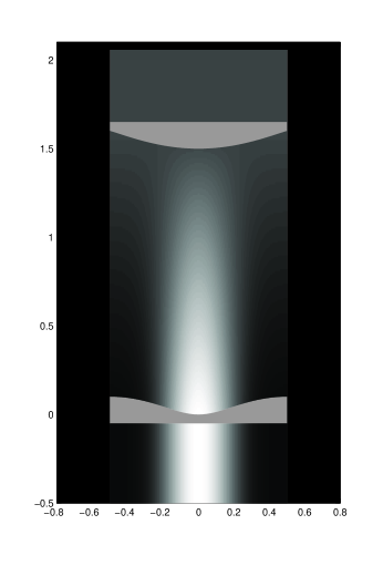
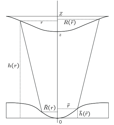
Figure 1: Pupil mapping via a pair of properly figured lenses.

Furthermore, if we consider the case of a pair of lenses that are plano on their outward-facing surfaces (as shown in Figure 1), then the inward-facing surface profiles, $h(r)$ and $\tilde{h}(\tilde{r})$, that are required to obtain the desired pupil mapping are given by the solutions to the following ordinary differential equations:

$$\frac{\partial h}{\partial r}(r)=\frac{r-\tilde{R}(r)}{\sqrt{Q_{0}^{2}+(n^{2}-1)(r-\tilde{R}(r))^{2}}},\qquad h(0)=z,$$ (2)

and

$$\frac{\partial\tilde{h}}{\partial\tilde{r}}(\tilde{r})=\frac{R(\tilde{r})-\tilde{r}}{\sqrt{\phantom{\tilde{|}}Q_{0}^{2}+(n^{2}-1)(R(\tilde{r})-\tilde{r})^{2}}},\qquad\tilde{h}(0)=0.$$ (3)

Here, $n$ is the refractive index and $Q_{0}$ is a constant determined by the distance $z$ separating the centers ($r=0$, $\tilde{r}=0$) of the two lenses: $Q_{0}=-(n-1)z$.

Let $S(r,\tilde{r})$ denote the distance between a point on the first lens surface $r$ units from the center and the corresponding point on the second lens surface $\tilde{r}$ units from its center. Up to an additive constant, the optical path length of a ray that exits at radius $\tilde{r}$ after entering at radius $r=R(\tilde{r})$ is given by

$$Q_{0}(\tilde{r})=S(R(\tilde{r}),\tilde{r})+n(\tilde{h}(\tilde{r})-h(R(\tilde{r}))).$$ (4)

In Vanderbei and Traub (2005), we showed that, for an on-axis source, $Q_{0}(\tilde{r})$ is constant and equal to $Q_{0}$.

2 High-Contrast Apodization

If we assume that an apodized beam with amplitude apodization profile $A(\tilde{r})$ such as one obtains as the output of a pupil mapping system is passed into an ideal imaging system with focal length $f$, the electric field $E(\rho)$ at the image plane is given by the Fourier transform of $A(\tilde{r})$:

$$E(\xi,\eta)=\frac{E_{0}}{\lambda f}\iint e^{2\pi i\frac{\tilde{x}\xi+\tilde{y}\eta}{\lambda f}}A(\sqrt{\tilde{x}^{2}+\tilde{y}^{2}})d\tilde{y}d\tilde{x}.$$ (5)

Here, $E_{0}$ is the input amplitude which, unless otherwise noted, we take to be unity. Since the optics are azimuthally symmetric, it is convenient to use polar coordinates. The apodization function $A$ is a function of $\tilde{r}=\sqrt{\tilde{x}^{2}+\tilde{y}^{2}}$ and the image-plane electric field depends only on image-plane radius $\rho=\sqrt{\xi^{2}+\eta^{2}}$:

$$E(\rho) = \frac{1}{\lambda f}\iint e^{2\pi i\frac{\tilde{r}\rho}{\lambda f}\cos(\theta-\phi)}A(\tilde{r})\tilde{r}d\theta d\tilde{r}$$ (6)

$$= \frac{2\pi}{\lambda f}\int J_{0}\left(2\pi\frac{\tilde{r}\rho}{\lambda f}\right)A(\tilde{r})\tilde{r}d\tilde{r}.$$ (7)

The point-spread function (PSF) is the square of the electric field:

$$\mbox{Psf}(\rho)=|E(\rho)|^{2}.$$ (8)

For the purpose of terrestrial planet finding, it is important to construct an apodization for which the PSF at small nonzero angles is ten orders of magnitude reduced from its value at zero. Figure 2 shows one such apodization function. In Vanderbei et al. (2003), we explain how these apodization functions are computed.

3 Huygens Wavelets

We have designed the pupil mapping system using simple ray optics but we have relied on diffraction theory to ensure that the apodization provides high contrast. This begs the question as to whether the desired high contrast will remain after a diffraction analysis of the entire system including the two-lens pupil mapping system or will diffraction effects in the pupil mapping system itself create “errors” that are great enough to destroy the high-contrast that we seek. To answer this question, we need to do a diffraction analysis of the pupil mapping system itself.

If we assume that a flat, on-axis, electric field arrives at the entrance pupil, then the electric field at a particular point of the exit pupil can be well-approximated by superimposing the phase-shifted waves from each point across the entrance pupil (this is the well-known Huygens-Fresnel principle—see, e.g., Section 8.2 in Born and Wolf (1999)). That is,

$$E_{\text{\scriptsize out}}(\tilde{x},\tilde{y})=\iint\frac{1}{\lambda Q(\tilde{x},\tilde{y},x,y)}e^{2\pi iQ(\tilde{x},\tilde{y},x,y)/\lambda}dydx,$$ (9)

where

$$Q(\tilde{x},\tilde{y},x,y)=\sqrt{(x-\tilde{x})^{2}+(y-\tilde{y})^{2}+(h(r)-\tilde{h}(\tilde{r}))^{2}}+n(Z-h(r)+\tilde{h}(\tilde{r}))$$ (10)

is the optical path length, $Z$ is the distance between the plano lens surfaces (i.e., a constant slightly larger than $z$), and where, of course, we have used $r$ and $\tilde{r}$ as shorthands for the radii in the entrance and exit pupils, respectively. As before, it is convenient to work in polar coordinates:

$$E_{\text{\scriptsize out}}(\tilde{r})=\iint\frac{1}{\lambda Q(\tilde{r},r,\theta)}e^{2\pi iQ(\tilde{r},r,\theta)/\lambda}rd\theta dr,$$ (11)

where

$$Q(\tilde{r},r,\theta)=\sqrt{r^{2}-2r\tilde{r}\cos\theta+\tilde{r}^{2}+(h(r)-\tilde{h}(\tilde{r}))^{2}}+n(Z-h(r)+\tilde{h}(\tilde{r})).$$ (12)

For numerical tractability, it is essential to make approximations so that the integral over $\theta$ can be carried out analytically. To this end, we need to make an appropriate approximation to the square root term:

$$S=\sqrt{r^{2}-2r\tilde{r}\cos\theta+\tilde{r}^{2}+(h(r)-\tilde{h}(\tilde{r}))^{2}}.$$ (13)

4 Fresnel Propagation

In this section we consider approximations that lead to the so-called Fresnel propagation formula.

If we assume that the lens separation is fairly large, then the $(h-\tilde{h})^{2}$ term dominates the rest and so we can use the first two terms of a Taylor series approximation (i.e., for $u$ small relative to $a$, $\sqrt{u^{2}+a^{2}}\approx a+u^{2}/2a$) to get the following large separation approximation:

$$S\approx(h(r)-\tilde{h}(\tilde{r}))+\frac{r^{2}-2r\tilde{r}\cos\theta+\tilde{r}^{2}}{2(h(r)-\tilde{h}(\tilde{r}))}.$$ (14)

If we assume further that the lenses are thin (i.e., that $n$ is large), then $h-\tilde{h}$ in the denominators can be approximated simply by $z$:

$$S\approx(h(r)-\tilde{h}(\tilde{r}))+\frac{r^{2}-2r\tilde{r}\cos\theta+\tilde{r}^{2}}{2z}.$$ (15)

This is called the thin lens approximation.

Combining the large lens separation approximation with the thin lens approximation, we get

$$E_{\text{\scriptsize out}}(\tilde{r})=\iint\frac{1}{\lambda Q_{1}(\tilde{r},r,\theta)}e^{2\pi iQ_{1}(\tilde{r},r,\theta)/\lambda}rd\theta dr$$ (16)

where

$$Q_{1}(\tilde{r},r,\theta)=\frac{r^{2}-2r\tilde{r}\cos\theta+\tilde{r}^{2}}{2z}+Z+(n-1)(Z-h(r)+\tilde{h}(\tilde{r})).$$ (17)

Finally, we simplify the reciprocal of $Q_{1}$ by noting that the $Z$ term dominates the other terms (i.e., for $u$ small relative to $a$, $1/(u+a)\approx 1/a$) and so we get that:

$$\frac{1}{Q_{1}(\tilde{r},r,\theta)}\approx\frac{1}{Z}.$$ (18)

This last approximation is called the paraxial approximation.

Combining all three approximations, we now arrive at the standard Fresnel approximation:

$$E_{\text{\scriptsize out}}(\tilde{r})=\frac{2\pi}{\lambda Z}e^{\pi i\frac{\tilde{r}^{2}}{z\lambda}+2\pi i\frac{(n-1)\tilde{h}(\tilde{r})}{\lambda}}\int e^{\pi i\frac{r^{2}}{z\lambda}-2\pi i\frac{(n-1)h(r)}{\lambda}}J_{0}(2\pi r\tilde{r}/z\lambda)rdr.$$ (19)

While the standard Fresnel approximation works very well in most conventional situations, it turns out (as well shall show) to be too crude of an approximation for high-contrast pupil mapping. It is inadequate because it does not honor the constancy of the optical path length $Q(\tilde{r},r,\theta)$ along the rays of ray-optics. That is, the fact that $Q(\tilde{r},R(\tilde{r}),0)$ is constant has been lost in the approximations. We should have used the ray-tracing optical path length as the “large quantity” in our large-lens-separation approximation instead of the simpler difference $h(r)-\tilde{h}(\tilde{r})$. But, this seemingly simple adjustment quickly gets tedious and so we prefer to take a completely different (and simpler) approach, which is described in the next section.

5 An Alternative to Fresnel

As we have just explained and shall demonstrate later, the standard Fresnel approximation does not produce good results for high-contrast pupil mapping computations. In this section, we present an alternative approximation that is slightly more computationally demanding but is much closer to a direct calculation of the true Huygens wavelet propagation.

As with Fresnel, we approximate the $1/Q(\tilde{r},r,\theta)$ amplitude-reduction factor in (11) by the constant $1/Z$ (the paraxial approximation). The $Q(\tilde{r},r,\theta)$ appearing in the exponential must, on the other hand, be treated with care. Recall that $Q(\tilde{r},R(\tilde{r}),0)$ is a constant. Since constant phase shifts are immaterial, we can subtract it from $Q(\tilde{r},r,\theta)$ in (11) to get

$$E_{\text{\scriptsize out}}(\tilde{r})\approx\frac{1}{\lambda Z}\iint e^{2\pi i(Q(\tilde{r},r,\theta)-Q(\tilde{r},R(\tilde{r}),0))/\lambda}rd\theta dr.$$ (20)

Next, we write the difference in $Q$’s as follows:

$$Q(\tilde{r},r,\theta)-Q(\tilde{r},R(\tilde{r}),0) = S(\tilde{r},r,\theta)-S(\tilde{r},R(\tilde{r}),0)+n(h(R(\tilde{r}))-h(r))$$ (21)

$$= \frac{S^{2}(\tilde{r},r,\theta)-S^{2}(\tilde{r},R(\tilde{r}),0)}{S(\tilde{r},r,\theta)+S(\tilde{r},R(\tilde{r}),0)}+n(h(R(\tilde{r}))-h(r))$$ (22)

and then we expand out the numerator and cancel big terms that can be subtracted one from another to get

$$S^{2}(\tilde{r},r,\theta)-S^{2}(\tilde{r},R(\tilde{r}),0) = (r-R(\tilde{r}))(r+R(\tilde{r}))-2\tilde{r}\left(r\cos\theta-R(\tilde{r})\right)$$ (23)

$$\qquad+\left(h(r)-h(R(\tilde{r}))\right)\left(h(r)+h(R(\tilde{r}))-2\tilde{h}(\tilde{r})\right).$$

When $r=R(\tilde{r})$ and $\theta=0$, the right-hand side clearly vanishes as it should. Furthermore, for $r$ close to $R(\tilde{r})$ and $\theta$ close to zero, the right-hand side gives an accurate formula for computing the deviation from zero. That is to say, the right-hand side is easy to program in such a manner as to avoid subtracting one large number from another, which is always the biggest danger in numerical computation.

So far, everything is exact (except for the paraxial approximation). The only further approximation we make is to replace $S(\tilde{r},r,\theta)$ in the denominator of (22) with $S(\tilde{r},R(\tilde{r}),0)$ so that the denominator becomes just $2S(\tilde{r},R(\tilde{r}),0)$. Putting this altogether and replacing the integral on $\theta$ with the appropriate Bessel function, we get a new approximation, which we refer to as the Huygens approximation:

$$E_{\text{\scriptsize out}}(\tilde{r}) \approx \frac{2\pi}{\lambda Z}\int e^{2\pi i\left(\frac{(r-R(\tilde{r}))(r+R(\tilde{r}))+2\tilde{r}R(\tilde{r})+\left(h(r)-h(R(\tilde{r}))\right)\left(h(r)+h(R(\tilde{r}))-2\tilde{h}(\tilde{r})\right)}{2S(\tilde{r},R(\tilde{r}),0)}+n(h(R(\tilde{r}))-h(r))\right)/\lambda}$$ (24)

$$\qquad\qquad\times J_{0}\left(2\pi\tilde{r}r/\lambda S(\tilde{r},R(\tilde{r}),0)\right)rdr.$$

6 Sanity Checks

In this section we consider a number of examples.

6.1 Flat glass windows ($A\equiv 1$)

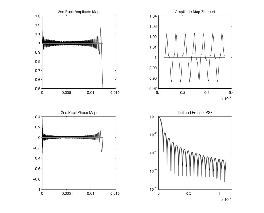
Figure 3: Fresnel analysis of a pupil mapping system consisting of two flat pieces of $n=1.5$ glass in circular $D=25$-mm apertures separated by $z=15D$. The wavelength is $\lambda=632.8$-nm. Upper-left plot shows in gray the target amplitude apodization profile and in black the amplitude profile computed using standard Fresnel propagation. Upper-right plot shows a zoomed in section of the amplitude profiles. Lower-left plot shows in gray the computed optical path length $Q_{0}(\tilde{r})$ and in black the phase map computed using Fresnel propagation. Lower-right plot shows in gray the PSF associated with the ideal amplitude apodization and in black the PSF computed by Fresnel propagation. These results should match textbook examples for simple open circular apertures—and they do.

We begin with the simplest example in which the apodization function is identically equal to one. Taking the positive root in (1), we get that $R(\tilde{r})=\tilde{r}$. That is, the ray-optic design is for the light to go straight through the system. The inverse map $\tilde{R}(r)$ is also trivial: $\tilde{R}(r)=r$. Hence, the right-hand sides in the differential equations (2) and (3) vanish and the lens figures become flat: $h(r)\equiv z$ and $\tilde{h}(\tilde{r})\equiv 0$. In this case, $Q_{1}(\tilde{r},R(\tilde{r}),0)$ is a constant (independent of $\tilde{r}$) and so the Fresnel approximation is a good one. The Fresnel results, shown in Figure 3 should match textbook examples for simple open circular apertures—and they do.

6.2 A Galilean Telescope ($A\equiv a>1$)

In this case, we ask for a system in which the output pupil has been uniformly amplitude intensified by a factor $a>1$. If we choose the positive root in (1), then we get a Galilean-style refractor telescope consisting of a convex lens at the entrance pupil and a concave lens as an eyepiece. Specifically, we get $R(\tilde{r})=a\tilde{r}$ and $\tilde{R}(r)=r/a$. From these it follows that if the aperture of the first lens is $D$, then the aperture of the second is $\tilde{D}=D/a$. It is easy to compute the lens figures

$$h(r) = z+\frac{\sqrt{Q_{0}^{2}+(n^{2}-1)(1-1/a)^{2}r^{2}}-|Q_{0}|}{(n^{2}-1)(1-1/a)}$$ (25)

$$\tilde{h}(\tilde{r}) = \frac{\sqrt{Q_{0}^{2}+(n^{2}-1)(a-1)^{2}\tilde{r}^{2}}-|Q_{0}|}{(n^{2}-1)(a-1)}.$$ (26)

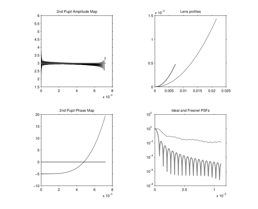
Figure 4: Same as in Figure 3 but with the apodization function replaced with a constant value of $A\equiv 3$. In this example, both lenses are hyperbolic as shown in the upper-right plot. The lens profiles $h$ and $\tilde{h}$ were computed using a $5,000$ point discretization and the Fresnel propagation (equation (19)) was carried out also with a $5,000$ point discretization. Note the large error in the phase map and the fact that the computed PSF does not follow the usual Airy pattern. This is strong evidence that the standard Fresnel approximation is too crude since real systems of this sort exist and exhibit the expected Airy pattern.

If the relative index of refraction $n$ is greater than $1$ (as in air-spaced glass lenses), then these functions represent portions of a hyperbola. If, on the other hand, $n<1$ (as in a glass medium between the two surfaces), then the functions are ellipses. Fresnel results for $a=3$ and $n=1.5$ are shown in Figure 4. Note the large error in the phase map and the fact that the computed PSF does not follow the usual Airy pattern. This is strong evidence that the Fresnel approximation is too crude since real systems of this sort exist and exhibit the expected Airy pattern.

In Figure 5 we consider the same system but use the Huygens approximation. Note that the phase map, while not perfect, is now much flatter. Also, the computed PSF is closely matches the expected Airy pattern.

6.3 An Ideal Lens

If we let $a$ tend to infinity, we see that $\tilde{D}$ tends to zero and the system reduces to a convex lens focusing a collimated input beam to a point. In this case, the second lens vanishes; only the first lens is of interest. Its equation is

$$h(r)=z+\frac{\sqrt{Q_{0}^{2}+(n^{2}-1)r^{2}}-|Q_{0}|}{(n^{2}-1)}.$$ (27)

The plane where the second lens was is now the image plane. To compute the electric field here, we put $\tilde{h}(\tilde{r})\equiv 0$ and use either the Fresnel or the Huygens approximation. Since we would put a detector at this plane, we can ignore any final phase corrections and both approximations reduce to the same formula:

$$E_{\text{\scriptsize out}}(\tilde{r})=\frac{2\pi}{\lambda Z}\int e^{\pi i\frac{r^{2}}{z\lambda}-2\pi i\frac{(n-1)h(r)}{\lambda}}J_{0}(2\pi r\tilde{r}/z\lambda)rdr.$$ (28)

Substituting (27) into (28) and dropping any unit complex numbers that factor out of the integral, we get

$$E_{\text{\scriptsize out}}(\tilde{r})=\frac{2\pi}{\lambda Z}\int e^{\pi i\frac{r^{2}}{z\lambda}-\frac{2\pi i}{\lambda}\sqrt{\left(\frac{n-1}{n+1}\right)^{2}z^{2}+\frac{n-1}{n+1}r^{2}}}J_{0}(2\pi r\tilde{r}/z\lambda)rdr.$$ (29)

Of course, this formula is for a uniform collimated input beam. If the input beam happens to be apodized by some upstream optical element, then the expression becomes

$$E_{\text{\scriptsize out}}(\tilde{r})=\frac{2\pi}{\lambda Z}\int e^{\pi i\frac{r^{2}}{z\lambda}-\frac{2\pi i}{\lambda}\sqrt{\left(\frac{n-1}{n+1}\right)^{2}z^{2}+\frac{n-1}{n+1}r^{2}}}J_{0}(2\pi r\tilde{r}/z\lambda)A(r)rdr$$ (30)

where $A(r)$ denotes the apodization function. This formula does not agree with the Fourier transform expression given earlier by equation (5). However, if the square root is approximated by the first two terms of its Taylor expansion,

$$\sqrt{\left(\frac{n-1}{n+1}\right)^{2}z^{2}+\frac{n-1}{n+1}r^{2}}=\frac{n-1}{n+1}z+\frac{r^{2}}{2z},$$ (31)

then (30) reduces to a Fourier transform as in (5) (again dropping unit complex factors).

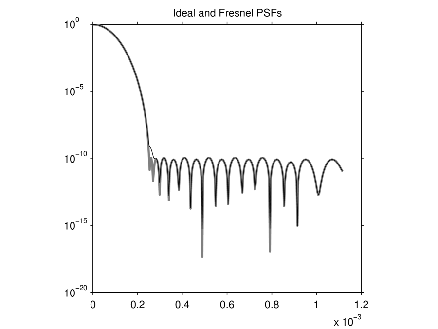
Figure 6: The gray plot shows an ideal high-contrast PSF designed assuming that the focussing element is a parabolic mirror so that the Huygens image-plane electric field is a Fourier transform as in equation (5). The black line shows the PSF if one assumes that the focussing element is actually an ideal lens (having an elliptical profile) as described in Section 6.3. The two curves are visually identical except in the neighborhood of the 1st and 2nd minima of the Fourier (gray) curve.

This raises an interesting question: if a high-contrast apodization is designed based on the assumption that the focusing element behaves like a Fourier transform (i.e., as in (5)), how well will the apodization work if the true expression for the electric field is closer to the one given by (30)? The answer is shown in Figure 6. The PSF degradation is very small.

7 High-Contrast Apodization

The purpose of the examples discussed in the previous section was to convince the reader that the Huygens approximation provides a reasonable estimate of the electric field at the exit pupil of a pupil mapping system. Assuming we were convincing, we now proceed to apply the Huygens approximation to compute the electric field and focused PSF of the pupil mapping system corresponding to the apodization function shown in Figure 2. As before, we assume a wavelength of $0.6328\mu$ and lenses with aperture $D=25$mm. In Figure 7, we show the results for $z=15D$ and a refraction index of $1.5$. For these simulations to be meaningful, it is critical that the integrals be represented by a sum over a sufficiently refined partition. The bigger the disparity between wavelength $\lambda$ and aperture $D$, the more refined the partition needs to be. For the parameters we have chosen, a partition into $5000$ parts proved to be adequate and is what we have chosen. The plot in the upper-left section of the figure shows in gray the target amplitude apodization profile and in black the amplitude profile computed using the Huygens approximation (i.e., equation (24)). The plot in the upper right shows the lens profiles. The first lens is shown in black and the second in gray. The plot in the lower left shows in gray the computed optical path length $Q_{0}(\tilde{r})$. If the numerical computation of the lens figures had been done with insufficient precision, this curve would not be flat. As we see, it is flat. The lower left also shows in black the phase map as computed by the Huygens approximation. Note that here there are high frequency oscillations everywhere and low frequency oscillation that has an amplitude that increases as one moves out to the rim of the lens. The lower-right plot shows in gray the PSF associated with the ideal amplitude apodization and in black the PSF computed by Huygens propagation.

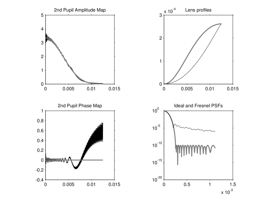
Figure 8: Same as in Figure 7 but computed using a brute force computation of the Huygens integral (11). Here we used $1000$ $r$-values and $1000$ $\theta$-values. Consequently, we needed to increase the wavelength by a factor $5$ to guarantee adequate sampling of the phase and amplitude ripples.

The PSF in Figure 7 is disappointing. It is important to determine whether this is real or is a result of the approximations behind the Huygens propagation formula. As a check, we did a brute force computation of the Huygens integral (11). Because this integral is more difficult, we were forced to use only 500 $r$-values and 500 $\theta$-values. Hence, we had to increase the wavelength by a factor of $10$. With these changes, the result is shown in Figure 8. It too shows the same amplitude and phase oscillations. This sanity check convinces us that these effects are physical. We need to consider changes to the physical setup that might mollify these oscillations. Such changes are considered next.

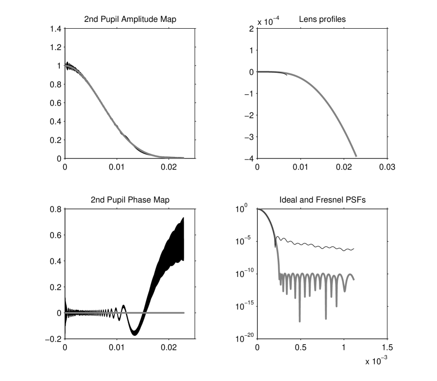
Figure 9: Same as in Figure 7 but with the apodization function normalized to a maximum value of one. This normalization results in the two lenses having different apertures, the second is about 4 times that of the first.

There is no particular reason to make the two lenses have equal aperture. By scaling the apodization function, we can easily generate examples with unequal aperture. One such experiment we tried was to scale the apodization function so that its value at the center is one. This scaling results in the second lens having almost four times the aperture of the first lens. The results for this case are shown in Figure 9.

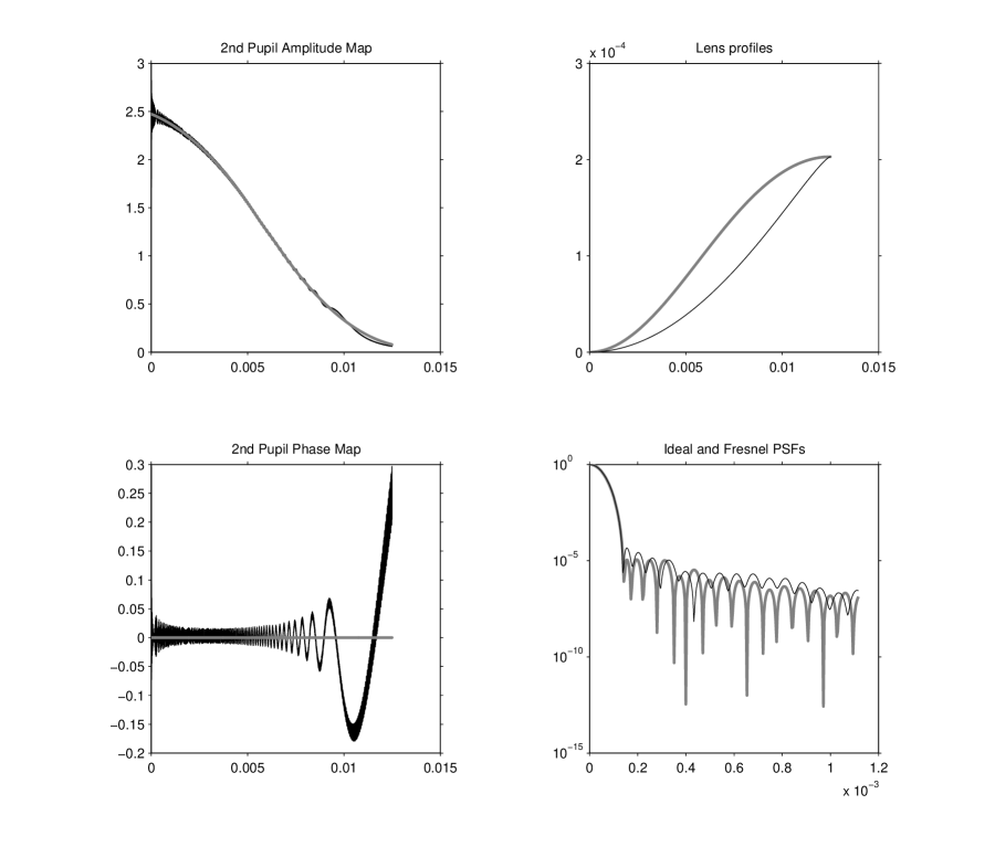
Figure 11: The various sanity checks suggest that diffraction effects fundamentally limit the close-in contrast attainable by pupil mapping to about $10^{-5}$. So, an apodization profile designed for $10^{-10}$ might not be the right one to use. Here, we show results for an apodization profile that only attempts to achieve $10^{-5}$. Note that the PSF via Huygens propagation (black) agrees fairly well with the ideal (Fourier transform) PSF (gray) in the lower-right plot.

If an apodization designed for $10^{-10}$ contrast only produces $10^{-5}$, one wonders how well an apodization designed for $10^{-5}$ will do. The answer is shown in Figure 11. In this case, the degradation due to diffraction effects is very small.

8 Hybrid Systems

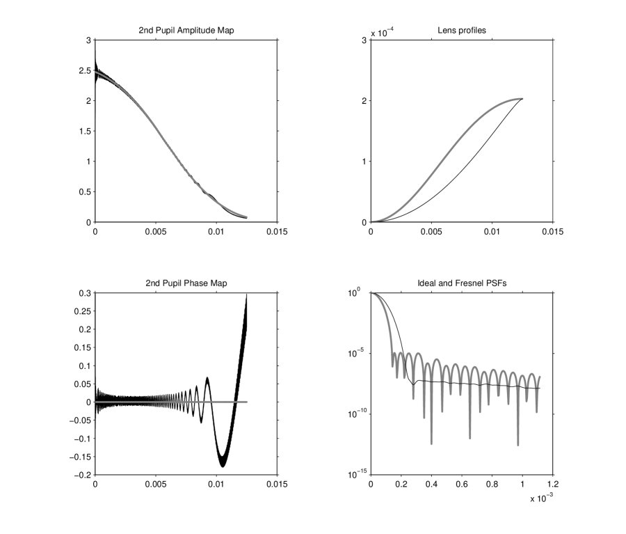
Figure 12: Given our success in Figure 11 of achieving $10^{-5}$ contrast with an apodization profile specifically designed for this level of contrast, we can now ask whether it is possible to put a conventional apodizer (or shaped pupil equivalent) in the exit pupil to further “convert” this apodization profile into one that achieves $10^{-10}$. The result is shown here. As seen in the PSF plots in the lower right, this combination gets the contrast to $10^{-7.5}$.

If a pupil mapping system designed for $10^{-5}$ works well, perhaps it could be followed by a conventional apodizer that attempts to bring the system from $10^{-5}$ down to $10^{-10}$. We tried this. The result is shown in Figure 12. As can be seen in the lower-right plot, the contrast achieved is limited to about $10^{-7.5}$. Apparently the diffraction ripples going into the apodizer are enough to prevent the system from achieving the desired contrast.

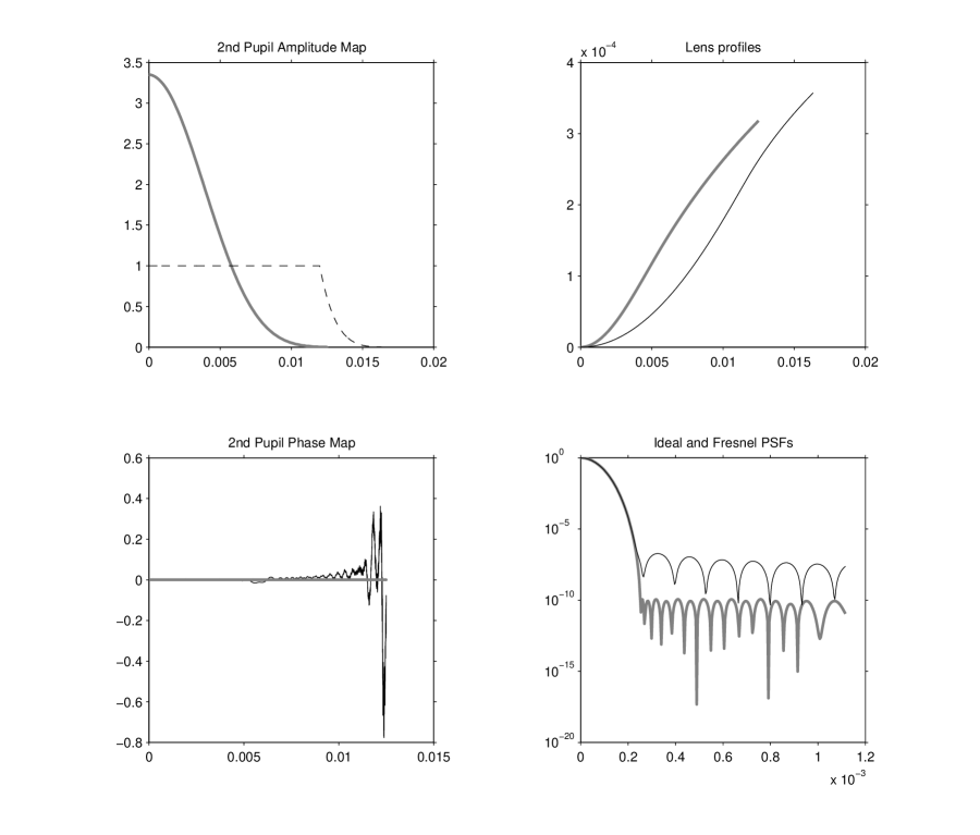
Figure 13: As an alternative to the back-end apodizer considered in Figure 12, we consider here the possibility of “softening” the edge of the first lens by using a pre-apodizer. The green curve in the upper-left plot shows the pre-apodization function we used. As one can see from the lower-right hand plot, this pre-apodization technique allows one to get the first side-lobe almost down to the $10^{-7}$ level. This result is not quite as good as what we had with the post-apodizer of Figure 12 but it is likely to be more manufacturable.

As an alternative to a downstream apodizer, one could consider a pre-apodizer placed in front of the first lens. Since it is generally hard edges that create bad diffraction effects, we can imagine using the pre-apodizer to provide the near-outer-edge apodization and allow the pupil mapping system to provide the main body of the apodization. In this way, perhaps the diffraction effects can be minimized while at the same time maintaining a system with high throughput. The results of one such experiment are shown in Figure 13.

Acknowledgements. This research was partially performed for the Jet Propulsion Laboratory, California Institute of Technology, sponsored by the National Aeronautics and Space Administration as part of the TPF architecture studies and also under JPL subcontract number 1260535. The first author received support from the NSF (CCR-0098040) and the ONR (N00014-98-1-0036).

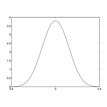
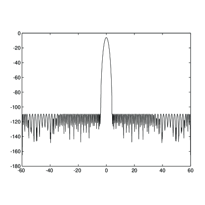
Figure 2: Left. An apodization providing contrast of $10^{-10}$ at tight inner working angles. Right. The corresponding on-axis point spread function.

Figure 5: Same as in Figure 4 but computed using the Huygens approximation. Note that the phase map, while not perfect, is now much flatter. Also, the computed PSF is closely matches the expected Airy pattern.

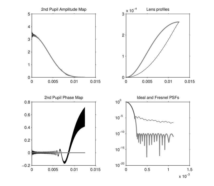
Figure 7: Analysis of a pupil mapping system using the Huygens approximation with $z=15D$ and $n=1.5$. Upper-left plot shows in gray the target amplitude apodization profile and in black the amplitude profile computed using the Huygens approximation. Upper-right plot shows the lens profiles, black for the first lens and gray for the second. The lens profiles $h$ and $\tilde{h}$ were computed using a $5,000$ point discretization. Lower-left plot shows in gray the computed optical path length $Q_{0}(\tilde{r})$ and in black the phase map computed using Huygens propagation. The Huygens propagation was carried out with a $5,000$ point discretization. Lower-right plot shows in gray the PSF computed as the square of the Fourier transform of the ideal amplitude apodization and in black the PSF computed using the Huygens approximation.

Figure 10: Same as in Figure 7 but with $75$mm lenses ($3$ times larger). The larger optical elements required a finer discretization of the integrals: $30,000$ points were used. The contrast improves but only marginally.

References

- Born and Wolf (1999) M. Born and E. Wolf. Principles of Optics. Cambridge University Press, New York, NY, 7th edition, 1999.
- Galicher et al. (2004) R. Galicher, O. Guyon, S. Ridgway, H. Suto, and M. Otsubo. Laboratory demonstration and numerical simulations of the phase-induced amplitude apodization. In Proceedings of the 2nd TPF Darwin Conference, 2004.
- Guyon (2003) O. Guyon. Phase-induced amplitude apodization of telescope pupils for extrasolar terrerstrial planet imaging. Astronomy and Astrophysics, 404:379–387, 2003.
- Traub and Vanderbei (2003) W.A. Traub and R.J. Vanderbei. Two-Mirror Apodization for High-Contrast Imaging. Astrophysical Journal, 599:695–701, 2003.
- Vanderbei et al. (2003) R.J. Vanderbei, D.N. Spergel, and N.J. Kasdin. Circularly Symmetric Apodization via Starshaped Masks. Astrophysical Journal, 599:686–694, 2003.
- Vanderbei and Traub (2005) R.J. Vanderbei and W.A. Traub. Pupil Mapping in 3-D for High-Contrast Imaging. Astrophysical Journal, 2005. To appear.