The peculiar velocities of satellites of external disk galaxies

Abstract

We analyze the angular distribution and the orbital rotation directions of a sample of carefully-selected satellite galaxies extracted from the Sloan Digital Sky Survey (SDSS). We also study these statistics in an $N$-body simulation of cosmological structure formation set within the $\Lambda$CDM paradigm under various assumptions for the orientations of disk angular momenta. Under the assumption that the angular momenta of the disks are aligned with the angular momenta of the inner regions of their host dark matter halos, we find that the fraction of simulated satellite halos that exhibit prograde motion is $f_{\mathrm{prog}}\approx 0.55-0.60$, with larger satellites more likely to be prograde. In our observational sample, approximately $60\%$ of the satellites exhibit prograde motion, a result that is broadly consistent with the simulated sample. Contrary to several recent studies, our observational sample of satellite galaxies show no evidence for being anisotropically distributed about their primary disks. Again, this result is broadly consistent with our simulated sample of satellites under the assumption that disk and halo angular momenta are aligned. However, the small size of our observational sample does not yet allow us to distinguish between various assumptions regarding the orientations of disks in their halos. Finally, we assessed the importance of contamination by interlopers on the measured prograde and retrograde statistics.

The Astrophysical Journal, submitted

1 Introduction

In the standard hierarchical, cold dark matter (CDM) scenario of cosmological structure and galaxy formation (e.g. White & Rees, 1978; Blumenthal et al., 1984), large systems are generally formed through the continual merging of comparably early-forming, low-mass objects in the hierarchy. In this context, the halos of large galaxies are formed by smaller halos that are accreted by the larger host and disrupted by tidal interactions. As the massive galactic halo is assembled, other halos and their associated galaxies may become gravitationally bound to the host and orbit in the host potential before possibly being incorporated into the central host galaxy or being strongly affected by tides (e.g. Taffoni et al., 2003; Hayashi et al., 2003; Zentner & Bullock, 2003; Kravtsov et al., 2004b; Kazantzidis et al., 2004b; Taylor & Babul, 2004; Zentner et al., 2005a).

The distribution of satellite galaxies about their primary galaxies has received significant attention, both theoretically and observational. A number of studies have focused on the radial distributions of satellite halos and satellite galaxies (e.g. Taylor et al., 2003; Zentner & Bullock, 2003; Kravtsov et al., 2004b; Diemand et al., 2004; Gao et al., 2004; van den Bosch et al., 2005; Zentner et al., 2005a; Nagai & Kravtsov, 2005); however, the angular distribution of satellites has become a subject of a great deal of recent activity. In an early study, Holmberg (Holmberg, 1969), found that satellites of spiral galaxies with projected separations $r_{\mathrm{p}}\lower 2.58334pt\vbox{\hbox{$\buildrel\textstyle<\over{\sim}\ $}}50\,{\mathrm{kpc}}$ are preferentially located near the short axes of the projected light distributions of their host galaxies. In other words, they are preferentially located near the poles of the primary disk galaxies. Zaritsky et al. (1997a) found a statistically-significant anisotropy, similar to that advocated by Holmberg (1969), at larger projected separations ($200\,{\mathrm{kpc}}\lower 2.58334pt\vbox{\hbox{$\buildrel\textstyle<\over{\sim}\ $}}r_{\mathrm{p}}\lower 2.58334pt\vbox{\hbox{$\buildrel\textstyle<\over{\sim}\ $}}500\,{\mathrm{kpc}}$) and, in a more recent study, Sales & Lambas (2004) found evidence for the preferential alignment of satellites along the minor axes of their primaries in the Two Degree Field Galaxy Redshift Survey (e.g. Colless et al., 2001). However, the observational status of the so-called Holmberg Effect is unclear. Brainerd (2004) studied satellites in the Sloan Digital Sky Survey (SDSS, e.g. York et al., 2000; Strauss et al., 2002) and found evidence for the opposite correlation of satellite position with the major axis of the light distribution of the primary galaxy.

Kroupa et al. (2005) recently reiterated that the satellite galaxies of the Milky Way (MW) are distributed anisotropically (see also Lynden-Bell, 1982; Majewski, 1994; Hartwick, 1996, 2000; Mateo, 1998; Grebel et al., 1999; Willman et al., 2004) and argued that this observation presents a challenge for the standard CDM paradigm. Zentner et al. (2005b, see also ; ; ;) showed that MW-sized dark matter halos contain satellite halos or subhalos that are distributed anisotropically about their central host halos. Subhalos are located preferentially near the long axes of their host dark matter halos, so that the anisotropy of MW satellites can be understood if the rotation axis of the MW disk is closely aligned with the long axis of the triaxial host dark matter halo of the MW. In order to test this alignment conjecture, it is necessary to examine a large sample of satellites about disk galaxy primaries.

Another interesting way to relate the properties of satellite galaxies to disk primaries is through the sense of rotation of the satellites relative to the disks, if any. On the theoretical side, the prediction for the number of prograde and retrograde satellites is unclear and there are many aspects to consider. In the simplest picture of disk galaxy formation, baryons in halos start off sharing the angular momentum distribution of their halos and, on average, conserve angular momentum as they cool and condense (e.g. Fall & Efstathiou, 1980). This implies that the poles of disk galaxies should be collinear with the net angular momentum vectors of their host halos which, in turn, are generally aligned with the halo minor axes (e.g. Warren et al., 1992; Porciani et al., 2002; Faltenbacher et al., 2005). Vitvitska et al. (2002, see also ) proposed that the angular momenta of dark matter halos are built through mergers with infalling satellite halos. If the accretion of satellites is a random process and the acquisition of angular momentum is a random walk as in the Vitvitska et al. (2002) model, this scenario seems to favor neither net prograde nor net retrograde satellite rotation because the angular momentum of the halo at disk formation may bear little resemblance to the angular momenta carried by the late-accreting satellites. However, the accretion of satellite halos generally occurs along a preferred direction, so that the accretion directions of satellites are strongly correlated (e.g. Knebe et al., 2004; Zentner et al., 2005b), the detailed consequences of which are unclear.

There are also dynamical processes that may affect the prograde and retrograde fractions of satellites subsequent to satellite accretion. Quinn & Goodman (1986) explored the idea that enhanced dynamical friction for satellites on nearly coplanar, prograde orbits about the disk could lead to enhanced destruction of prograde satellites but found this process to be fairly inefficient. Peñarrubia et al. (2002) extended this to include the effect of an oblate halo about the disk; however, their result was that preferred destruction is inefficient for satellites further than $\sim 50\,{\mathrm{kpc}}$ from the primary because the orbital decay times are large at these radii (see also Zaritsky & Gonzalez, 1999). Moreover, CDM halos generally tend to be more prolate rather than oblate (e.g. Jing & Suto, 2002; Bullock, 2002; Kazantzidis et al., 2004a). Another dynamical argument relates to the heating of galactic disks. Velázquez & White (1999) conducted self-consistent $N$-body simulations of satellites interacting with disk galaxies and found that massive satellites may be accreted without destroying the primary disk galaxy, particularly for satellites on retrograde orbits which produce significantly less disk heating than satellites on prograde orbits.

¿From an observational point of view, Carignan et al. (1997) found that seven satellites around the giant lenticular galaxy NGC5084 exhibit retrograde motion while only one satellite is prograde. Moreover, the large mass and the tilted disk of NGC5084 suggest that this galaxy has survived a number of mergers, possibly with prograde satellites. Similarly, Zaritsky et al. (1997b) examined the orbits of their sample of satellites about disk galaxies and found that a slight excess ($52\%$) of satellites exhibit retrograde motions in a sample of $69$ primaries with $115$ satellites.

Any statistical work on satellite galaxies has to face the problem of the small average number of satellites that can be identified for each primary (e.g. Zaritsky et al., 1997b; McKay et al., 2002; Prada et al., 2003). Provided that the primary galaxies are selected in a consistent and homogeneous way, it is useful to consider all satellites in the sample as satellites of a single, fictitious primary. This is the assumption that we work under here.

In this paper we use a sample of hosts and satellites extracted from the SDSS (Prada et al., 2003) and a sample of halos and subhalos in a cosmological $N$-body simulation in order to address a number of questions concerning the angular momenta of disk galaxies relative to their satellites as follows.

1. What is the distribution of angular distances of satellites from the planes of the primary disk galaxies and how does this compare to the theoretically-predicted angular distribution of satellite halos in simulations of structure formation in the context of CDM?

2. What is the ratio between prograde and retrograde satellites ($P/R$) in a well-defined sample of observed satellite systems and how does this compare to predicted satellite orbits?

3. Does the fraction of prograde satellites depend on the angular distance of the satellites from the plane of the primary disk or with projected physical separation?

4. How does the presence of interlopers (objects that are field galaxies, not dynamically bound to the primary, but counted as satellites due to projection) affect $P/R$ in our observational sample relative to the value for “true” satellites?

This manuscript is organized as follows. In the next section, we describe the numerical simulations and analysis methods that we use to compute theoretical predictions for satellite distributions and present the basic results from the simulation. We describe our data and present the observational results in § 3. In § 4, we discuss the effects of interlopers and observational biases. Finally, we present our results and draw our conclusions in § 5. The main sample from which our objects are extracted (see Prada et al., 2003) was compiled using $B$ magnitudes, therefore, throughout this paper, we refer exclusively to $B$ magnitudes, either apparent or absolute.

2 Theoretical Predictions

2.1 Numerical Simulation

To compare the observed satellite sample to the theoretically-predicted distributions of satellites in the context of CDM, we analyzed a simulation of structure formation in the so-called concordance cosmological constant plus CDM cosmology ($\Lambda$CDM), with $\Omega_{M}=0.3$, $\Omega_{\Lambda}=0.7$, $h=0.7$, $\Omega_{B}h^{2}=0.22$, $n_{\mathrm{s}}=1$, and a power spectrum normalization of $\sigma_{8}=0.9$. The simulation followed the evolution of $512^{3}$ particles in a computational box of $80\,{h^{-1}\mathrm{Mpc}}\simeq~{}114.3\,{\mathrm{Mpc}}$ on a side, implying a particle mass of $m_{\mathrm{p}}\simeq~{}3.16\times 10^{8}\,{h^{-1}\mathrm{M}_{\odot}}$.

The simulation was performed using the Adaptive Refinement Tree $N$-body simulation code (ART Kravtsov et al., 1997; Kravtsov, 1999). The ART code employs a particle-mesh approach and achieves high force resolution by refining the grid in all high-density regions with a recursive refinement algorithm. This creates an hierarchy of refinement meshes of different resolution covering regions of interest. The mesh cells were refined up to a maximum of eight levels, corresponding to a minimum cell size of $h_{\mathrm{peak}}\simeq~{}1.22\,{h^{-1}\mathrm{kpc}}$.

We identified halos and subhalos using a variant of the Bound Density Maxima algorithm (Klypin et al., 1999). We began by computing the local density at each particle using a smoothing kernel of $24$ particles and identified local maxima in the density field. We proceeded through all density peaks, beginning with the highest density peak and moving toward lower density, and marked each peak as a potential halo center. We surrounded each such peak with a sphere of radius $r_{\mathrm{find}}=20\,{h^{-1}\mathrm{kpc}}$ and excluded all particles within this sphere from further consideration as a potential halo center. The parameter $r_{\mathrm{find}}$ is determined by the size of the smallest halos that we aim to identify robustly. After identifying potential halo centers, we iteratively removed unbound particles.

We used the remaining bound particles to compute the circular velocity profile of the halo $V_{\mathrm{circ}}=\sqrt{GM(<r)/r}$, and the maximum circular velocity $V_{\mathrm{max}}$. We defined the virial masses and radii of halos corresponding to a fixed, spherical overdensity of $\Delta=180$ times the mean density of the universe $\rho_{\mathrm{M}}$, so that $M_{180}\equiv 4\pi(\Delta\rho_{\mathrm{M}})R_{180}^{3}/3$ . For satellite halos or subhalos that are self-bound substructures within the virial radius of a larger parent or host halo, the outer boundary is somewhat ambiguous. We adopted a truncation radius $r_{\mathrm{t}}$, at which the slope of the density profile became greater than a critical value of $\mathrm{d}\ln\rho/\mathrm{d}\ln r=-0.5$. This criterion was based on the fact that we do not expect density profiles of CDM halos to be shallower than this and, empirically, this definition is approximately equal to the radius at which the background density of the host halo particles is equal to the density of the particles bound to the subhalo. In what follows, we choose to quantify the size of halos and subhalos according to the peak circular velocity $V_{\mathrm{max}}$, because for subhalos this quantity is measured more robustly and this quantity is not subject to the same ambiguity as any particular mass definition.

2.2 Analysis Methods

One of our goals is to compare the observed statistics of satellite galaxies to theoretical predictions using the catalogs of observed satellites and primaries described in § 3. In order to do this, we construct catalogs of galaxies with absolute $B$ magnitudes from the halos and subhalos of the simulation. There are several empirical methods to connect galaxies to halos that have been explored in the recent literature (e.g. Seljak, 2000; Berlind & Weinberg, 2002; Yang et al., 2003; van den Bosch et al., 2003a, b; Zheng et al., 2004; van den Bosch et al., 2005). For simplicity, we assign magnitudes to halos using the prescription advocated by Kravtsov et al. (2004a) in their study of galaxy and halo clustering statistics. We map magnitudes onto halos by requiring the number density of halos with maximum circular velocities greater than some $V_{\mathrm{max}}$ to be equal to the observed number density of galaxies with absolute $B$ magnitudes greater than some corresponding $M_{\mathrm{B}}(V_{\mathrm{max}})$. To compute the number densities of galaxies of a given magnitude, we used the Schechter (1976) function fits to the SDSS $g$-band luminosity function presented in Blanton et al. (2003). To convert from $g$ to $B$, we used the conversions compiled by M. Blanton at URL http://cosmo.nyu.edu/blanton/kcorrect/. The resulting correspondence between halo $V_{\mathrm{max}}$ and $M_{\mathrm{B}}$ is shown in Figure 1, where we also show the number density of halos as a function of $V_{\mathrm{max}}$. Kravtsov et al. (2004a) showed that a similar mapping of galaxies onto halos using $r$-band luminosities reproduces the clustering statistics of galaxies as a function of luminosity as measured by the SDSS.

Figure 1: Assigning magnitudes to halos in the $N$-body simulation. The horizontal axis is the maximum circular velocity of halos and subhalos $V_{\mathrm{max}}$. The decreasing function of $V_{\mathrm{max}}$ is the number density of halos as a function of maximum circular velocity, $n(V_{\mathrm{max}})$. This line should be read against the vertical axis on the right side of the plot. The increasing function of $V_{\mathrm{max}}$ is the absolute $B$ magnitude $M_{\mathrm{B}}$, of galaxies with the same number density as the number density of halos at this value of $V_{\mathrm{max}}$ (decreasing line). This line should be read against the vertical axis on the left side of the plot and it represents the mapping of halo size ($V_{\mathrm{max}}$) to absolute magnitude ($M_{\mathrm{B}}$) that we use to compare our observational results to halos and subhalos in dissipationless simulations.

For each primary halo in the catalogs, we computed reference vectors that allow us to orient satellites relative to halos in a meaningful way. To compute these vectors, we used all primary halo particles within $R\leq 0.3R_{180}$ in order to mitigate the influence of large substructures at large halo-centric distances on these vectors and to focus on the properties of the inner halo which contains the material that collapsed earliest and where any disk galaxy would reside. First, we computed the principal axes of the triaxial primary halos using an iterative algorithm as described in detail in Zentner et al. (2005b, see also ; ). We also computed the net angular momentum vector of all primary halo particles within $R\leq 0.3R_{180}$. In the following, we compare various hypotheses for the orientations of disks in their primary halos to the data regarding the relative positions and velocities of satellite galaxies in our sample. We computed all statistics by summing over three orthogonal projections through the simulation volume and we computed statistical errors by taking each projection to be statistically independent.

2.3 Theoretical Predictions

After assigning magnitudes to halos and determining reference vectors for halos, we constructed catalogs of primaries and satellites by observing the simulation from three orthogonal projection directions using the same criteria as we employed for our observational sample (see § 3.1 below). Primaries were restricted to only those halos that are assigned magnitudes $-20.5\leq M_{\mathrm{B}}\leq-19.5$. Primaries were required to satisfy isolation criteria such that any halos with projected separations $r_{\mathrm{p}}\leq 500\,{h^{-1}\mathrm{kpc}}$ and line-of-sight velocity differences $\Delta V\leq 1000{\,{\mathrm{km}}\,{\mathrm{s}}^{-1}}$ with respect to the primary are dimmer by at least $\Delta M_{\mathrm{B}}\geq 2$. Satellites were required to have $\Delta M_{\mathrm{B}}\geq 2$, $r_{\mathrm{p}}\leq 350\,{h^{-1}\mathrm{kpc}}$, and $\Delta V\leq 500{\,{\mathrm{km}}\,{\mathrm{s}}^{-1}}$.

The first results from the simulations concern the angular positions of the observed satellites. We have examined three idealized hypotheses regarding the orientation of disks in dark matter halos: (1) that the disk rotation axis is aligned with the angular momentum of the halo; (2) that the disk is aligned with the major axis of the host halo; (3) that the disk is aligned with the minor axis of the halo (which is generally in close alignment with the angular momentum axis). The first hypothesis is based recent attempts to reconcile the anisotropic of distribution of satellites in the Local Group (e.g. Lynden-Bell, 1982; Hartwick, 2000; Willman et al., 2004; Kroupa et al., 2005) with the predictions of numerical simulations (e.g. Zentner et al., 2005a; Libeskind et al., 2005). Alternatively, the simplest picture of disk galaxy formation predicts that halo and disk angular momenta should be nearly aligned (Fall & Efstathiou, 1980, though cosmological hydrodynamic simulations show a misalignment of baryon and dark matter angular momenta that is typically $\sim 10^{\circ}-20^{\circ}$, see van den Bosch et al. 2002; Chen et al. 2003). We have defined the angle $\phi$ as the angle between the long axis of the primary disk and the position of the satellite in two-dimensional projection.

The cumulative angular distributions are shown in Figure 2. In the case where the disk is closely aligned with the major axis of the primary halo (solid lines), the anisotropy is apparent as a deficit of satellites at small and intermediate angles in Figure 2. In this scenario, satellites are located preferentially near the short axes of their disk primaries in a sense similar to that observed by Holmberg (1969), Zaritsky et al. (1997a), and Sales & Lambas (2004). A Kolmogorov-Smirnov (KS) test reveals that the probabilities for the simulated samples with $M_{\mathrm{B}}\leq-16.5$ and $M_{\mathrm{B}}\leq-15.5$ to be drawn from an isotropic underlying distribution are $P_{\mathrm{KS}}\simeq~{}9\times 10^{-5}$ and $P_{\mathrm{KS}}\simeq~{}5\times 10^{-5}$ respectively. In Figure 2, we also show the resulting distributions under the assumption that disk rotation is aligned with the angular momentum axis of the inner halo of the primary. Under this assumption, their appears to be a very slight excess of satellites at small and intermediate angles, but the distributions are consistent with isotropy. The distributions with the disk angular momenta aligned with halo minor axes are quite similar to these and we have omitted them from Figure 2 in the interest of clarity.

Figure 2: The cumulative angular distribution of satellites relative to the long axes of their primaries in simulations. The three panels correspond to three different magnitude limits, $M_{\mathrm{B}}\leq-17.5$, $M_{\mathrm{B}}\leq-16.5$, and $M_{\mathrm{B}}\leq-15.5$ from top to bottom. Solid lines correspond to the assumption that the disk rotation axis is aligned with the major axis of the primary halo. Dashed lines correspond to the assumption that the disk rotation axis is aligned with the angular momentum of the inner halo of the primary. The straight, dotted lines correspond to an isotropic distribution in $\phi$. In the lower right of each panel, we give the KS probability for the satellites in the samples with disk rotation along the major axis of the halo to be drawn from an isotropic distribution. In all cases, the simulated samples with disk rotation aligned with halo angular momentum are consistent with isotropy.

The next results concern the fraction of satellites that exhibit prograde or retrograde motion with respect to the disk of the primary galaxy. In the case of the alignment of disk rotation with the major or minor axes of the host halo, there is no obvious way to assign a sense to the rotation to the disk. For this reason, we have computed prograde and retrograde statistics only for the case where the direction of the disk rotation is assumed to be aligned with the net angular momentum vector of the dark matter of the primary halo within $R<0.3R_{180}$. The results are summarized in Table 1. The error estimates listed in Table 1 represent the standard deviation of a binomial distribution with the appropriate parameters for each case. By presenting the prograde/retrograde statistics in this way, we have assumed that we can treat the three projections through the simulation as independent. The excess of prograde satellites is a robust prediction in this scenario. Additionally, notice the trend for larger satellites to have a greater probability to exhibit prograde relative motion. For example, the satellites in the largest bin show a significant trend toward prograde motion as do the satellites with $-17.5\geq M_{\mathrm{B}}\geq-18.0$, where there are $247$ satellites with $141$ progrades, yielding $f_{\mathrm{prog}}=0.57\pm 0.03$. Alternatively, in the magnitude range $-15.5\geq M_{\mathrm{B}}\geq-16.0$, there are $294$ satellites, $152$ of which are prograde, yielding a prograde fraction in this bin of luminosity of $f_{\mathrm{prog}}=0.52\pm 0.03$.

Table 1: Prograde and Retrograde Satellites In Simulations

$V_{\mathrm{max}}$	$M_{\mathrm{B}}$	$N_{\mathrm{sats}}$	$N_{\mathrm{prog}}$	$N_{\mathrm{retr}}$	$f_{\mathrm{prog}}$
${\,{\mathrm{km}}\,{\mathrm{s}}^{-1}}$
$98.2$	$-18.0$	$81$	$53$	$28$	$0.65\pm 0.05$
$91.5$	$-17.5$	$328$	$194$	$134$	$0.59\pm 0.03$
$86.4$	$-17.0$	$647$	$360$	$287$	$0.56\pm 0.02$
$82.4$	$-16.5$	$925$	$502$	$423$	$0.54\pm 0.02$
$78.8$	$-16.0$	$1226$	$670$	$556$	$0.55\pm 0.01$
$75.9$	$-15.5$	$1520$	$822$	$698$	$0.54\pm 0.01$

The prograde and retrograde fractions of satellites in the simulation volume. Column description: (1) The minimum value of $V_{\mathrm{max}}$ for satellites in the sample in ${\,{\mathrm{km}}\,{\mathrm{s}}^{-1}}$; (2) The corresponding maximum magnitude determined by matching halo number densities to galaxy number densities; (3) The total number of satellites in the sample, summed over the three, orthogonal projections through the simulation volume; (4) The number of prograde satellites that have peculiar velocities that are in the same direction as the rotation of the inner halo; (5) The number of retrograde satellites that have peculiar velocities that are in the opposite direction of the rotation of the inner dark matter halo; (6) The fraction of satellites with prograde velocities.

The excess of prograde satellites and the trend toward higher prograde fractions for larger satellites are not altogether surprising. CDM halos tend to be connected through a network of filamentary structures established by the statistics of the density field and the tidal field during collapse in overdense regions (e.g. Klypin & Shandarin, 1983; Bond & Myers, 1996; Bond et al., 1996; Colberg et al., 2004). The matter distribution within the filaments is strongly concentrated toward the axis of the filament (Colberg et al., 2004) and halos preferentially tend to form in these dense regions and then merge along the dominant filamentary directions. This leads to a strong correlation between directions along which halos merge during the mass accretion history of the primary halo (Knebe et al., 2004; Zentner et al., 2005b). The subhalos that merge early and establish the angular momentum of the inner regions of the primary halo (e.g. Vitvitska et al., 2002) flow along directions that are similar to the directions of infalling subhalos at late times, which are then observed as the satellites. Larger halos tend to be more strongly biased toward formation in the overdense regions (e.g. Bond & Myers, 1996; Bond et al., 1996), so they are more faithful tracers of the flow along the filaments. The higher prograde fractions for larger satellites are a reflection of this.

Figure 3: The peculiar velocities of the simulated satellite samples relative to the angular momenta of the central regions of the primary host halos. The histograms show the fraction of satellites in bins of peculiar velocity with retrograde satellites on the left (negative peculiar velocity relative to the disk) and prograde satellites on the right. The vertical, dashed line shows the separation between prograde and retrograde satellites at zero peculiar velocity. We show histograms for three subsamples labeled by both their minimum $V_{\mathrm{max}}$ and their maximum $M_{\mathrm{B}}$. The solid line is $V_{\mathrm{max}}\geq 76{\,{\mathrm{km}}\,{\mathrm{s}}^{-1}}$ ($M_{\mathrm{B}}\leq-15.5$), the dotted line is for $V_{\mathrm{max}}\geq 82{\,{\mathrm{km}}\,{\mathrm{s}}^{-1}}$ ($M_{\mathrm{B}}\leq-16.5$), and the dashed line is for $V_{\mathrm{max}}\geq 92{\,{\mathrm{km}}\,{\mathrm{s}}^{-1}}$ ($M_{\mathrm{B}}\leq-17.5$).

The excess of prograde satellites is also shown in Figure 3, which is a histogram of the peculiar velocities of the simulated satellite halos with respect to their primaries. In this plot, positive peculiar velocities are defined to be in the same sense as the rotation of the disk. Again, the modest excess of prograde satellites, particularly with relatively small peculiar velocities, is apparent.

The simulated catalog provides a tool to study the effect of interlopers on the prograde/retrograde fractions because in this case we know both the “observed” sample and the true three-dimensional separation. We have taken as a working definition to separate true satellites from interlopers a three-dimensional distance of $r_{\mathrm{true}}=1\,{h^{-1}\mathrm{Mpc}}$. Satellites that are a distance greater than $r_{\mathrm{true}}$ from their primaries are considered interlopers. The virial radii of primaries in our sample range from roughly $175\,{h^{-1}\mathrm{kpc}}$ to $400\,{h^{-1}\mathrm{kpc}}$, so we generally expect objects at distances greater than $\sim 1\,{h^{-1}\mathrm{Mpc}}$ to be unrelated to the primary. In Table 2, we show the prograde/retrograde fractions for the true satellites separated in three-dimensions by a distance less than $r_{\mathrm{true}}$, with no contamination by interlopers. We find that the net effect of interlopers at large line-of-sight separations is to dilute the prograde/retrograde fractions by $\sim 1-7\%$, depending upon the details of the sample selection.

Table 2: Prograde and Retrograde Satellites In Simulations with Interlopers Removed

$M_{\mathrm{B}}$	$N_{\mathrm{prog}}$	$N_{\mathrm{retr}}$	$f_{\mathrm{prog}}$	$f_{\mathrm{false}}$
$-18.0$	$42$	$16$	$0.72\pm 0.06$	$0.29$
$-17.5$	$145$	$90$	$0.62\pm 0.03$	$0.29$
$-17.0$	$278$	$196$	$0.59\pm 0.02$	$0.27$
$-16.5$	$385$	$291$	$0.57\pm 0.02$	$0.26$
$-16.0$	$499$	$389$	$0.56\pm 0.02$	$0.27$
$-15.5$	$608$	$496$	$0.55\pm 0.02$	$0.27$

The prograde and retrograde fractions of satellites with true, three-dimensional distances smaller than $r_{\mathrm{true}}=1\,{h^{-1}\mathrm{Mpc}}$ from their associated primaries in the simulation volume. Column description: (1) The corresponding maximum magnitude determined by matching halo number densities to galaxy number densities; (2) The number of prograde satellites that have peculiar velocities that are in the same direction as the rotation of the inner halo; (3) The number of retrograde satellites that have peculiar velocities that are in the opposite direction of the rotation of the inner dark matter halo; (4) The fraction of prograde satellites; (5) The fraction of all satellites in Table 1 that were identified as “false” satellites at each magnitude threshold, defined by the fact that they were included in the sample due to projection effects but are a distances greater than $r_{\mathrm{true}}=1\,{h^{-1}\mathrm{Mpc}}$ from their primaries.

3 Observational Results

3.1 The Observed Sample

Our observed sample of systems is extracted from “Sample 2” of Prada et al. (2003), which was constructed from SDSS data. Sample 2 has a maximum depth of $60000{\,{\mathrm{km}}\,{\mathrm{s}}^{-1}}$ and a limiting absolute magnitude in $B$ of $M_{\mathrm{B}}=-18$. The isolation criteria of the primaries in the sample are that any satellites within a projected radial separation of $r_{\mathrm{p}}\leq 500\,{h^{-1}\mathrm{kpc}}$ and with a line-of-sight velocity difference $\Delta V\leq 1000{\,{\mathrm{km}}\,{\mathrm{s}}^{-1}}$ must be dimmer than the primary by at least $\Delta M_{\mathrm{B}}\geq~{}2$. Satellites must satisfy $\Delta M_{\mathrm{B}}\geq~{}2$ with respect to their associated primary, they must have a projected distance to the primary of $r_{\mathrm{p}}\leq 350\,{h^{-1}\mathrm{kpc}}$, and a line-of-sight velocity difference of $\Delta V\leq 500{\,{\mathrm{km}}\,{\mathrm{s}}^{-1}}$.

Sample 2 contains more than $700$ primaries and more than $1000$ satellites. Using Sample 2 as a starting point, we selected our primaries according to the following additional criteria.

1. We enforced a limiting depth of $11000{\,{\mathrm{km}}\,{\mathrm{s}}^{-1}}$.

2. We chose primaries only in the magnitude range $-20.5\leq M_{\mathrm{B}}\leq-19.5$

3. We required all primaries to have a well-defined morphological type as a spiral.

The limit of $11000{\,{\mathrm{km}}\,{\mathrm{s}}^{-1}}$ was imposed not to lose too many satellites, as the SDSS is complete down to $M_{\mathrm{B}}=-17.5$ at $11000{\,{\mathrm{km}}\,{\mathrm{s}}^{-1}}$, thus the satellites (two magnitudes fainter than primaries) are those brighter than $M_{\mathrm{B}}=-15.5$ only. The narrow magnitude range for the primaries was chosen to avoid including primaries with very different masses, given the known dependence of luminosity on the mass of the primary (e.g. Prada et al., 2003). Further, satellites with projected distances from their primaries smaller than $20\,{\mathrm{kpc}}$ were rejected, due to potential galaxy misclassification (e.g. HII region contamination, bright stars etc.). After applying these constraints, we were left with $144$ spiral primaries and $193$ satellites. We obtained the direction of rotation of a limited number of primaries, so we analyzed the prograde and retrograde motion using a subsample of $43$ primary galaxies with $76$ satellites (see § 3.3). For the angular distribution analysis, we used the entire sample of $193$ satellites (see § 3.2).

Table 3: The Primaries and Satellites of the sample.

Name	Bmag	RA(2000)	DEC(2000)	PA	V(${\,{\mathrm{km}}\,{\mathrm{s}}^{-1}}$)	$\Delta V$	dist (kpc)	Orbit
pgc001112	-20.3	00 16 55	-00 05 18	170	10042.9	-	-	-
a	-18.3	00 17 07	-00 08 30	137	10098.7	55.8	175.1	r
pgc001841	-20.1	00 30 07	-11 06 49	169	3649.6	-	-	-
a	-15.9	00 31 28	-10 40 33	37	3645.2	-4.4	486.0	p
mcg-2-3-61	-20.2	01 00 04	-11 04 56	123	5519.4	-	-	-
a	-17.9	01 00 05	-11 02 32	6	5420.0	-99.4	52.2	r
ngc341	-20.4	01 00 45	-09 11 08	55	4658.0	-	-	-
a	-16.9	01 01 43	-09 19 00	119	4639.3	-18.7	294.5	p
ugc1962	-20.0	02 28 54	00 22 13	105	6152.9	-	-	-
b	-17.4	02 29 33	00 22 23	91	6549.3	396.4	240.4	p
c	-17.0	02 29 39	00 07 23	37	6155.4	2.5	455.2	p

The observational data listed in Table 3 come from the SDSS database and from our own observations with the exception of NGC2841, which had a previously-published rotation curve that we took from Afanasiev & Silchenko (1999). Data such as recessional velocities, absolute magnitudes and positions for primaries and satellites were taken from the SDSS database, while the Position Angles of the primaries were taken from the Lyon-Meudon Extragalactic Database (LEDA) . Low-resolution spectroscopy of the H$\alpha$ line easily determines the spin direction of our objects. Therefore, through an observational program at the telescopes of the Isaac Newton Group (La Palma, Canary Islands), we obtained rotational data for $42$ of our primaries.

Observations were performed using the spectrographs ISIS, of the $4.2$ m William Herschel Telescope (WHT), and IDS, of the $2.5$ m Isaac Newton Telescope (INT) of the Isaac Newton Group, on La Palma, Spain. The setup was simple and no special observing conditions were needed, so most of the data were taken in service mode. The most important aspect of the observation was to determine reliably the orientation of the charge-coupled device (CCD), to be able to place the receding end of the galaxies correctly on the sky. Two exposures at Sky PA $0^{\circ}$, shifted by some $10\arcsec$, and two more at Sky PA $90^{\circ}$ with the same offset were sufficient to mark North and East on the images.

We used the R316R or R600R gratings on the Marconi II chip with ISIS, centered at $6650\AA$, and R900V, R600V on chip EEV13 or R1200R on chip EEV10 with IDS, also centered at $6650\AA$. The slit width ranged from $1\arcsec$ to $1.5\arcsec$, depending on the seeing conditions. Exposure times were typically $300\,{\mathrm{s}}$ with WHT and $900\,{\mathrm{s}}$ with INT. During the observations, the seeing varied from $0.8\arcsec$ up to $2.5\arcsec$. The detection of the shift on the H$\alpha$ line was performed by analyzing the images with the IRAF package, comparing the line centroid shift with that of a sky line to correct for spurious rotations of the CCD. The observing runs took place over the period from March to September of 2003.

3.2 The Angular Distribution of Satellites

In order to study the distribution of the angular positions of the observed satellites relative to their disk primaries we were able to use our largest sample of objects because this requires only the coordinates of all objects and the Position Angles of the primaries, which we extracted from the LEDA database. We included in this analysis the $144$ disk primaries in the magnitude bin $-20.5\leq M_{\mathrm{B}}\leq-19.5$, and the $193$ satellites selected according to the description in § 3.1. We reduced the angular distance of the satellites from the disks to a single quadrant, $\phi\in[0^{\circ},90^{\circ}]$.

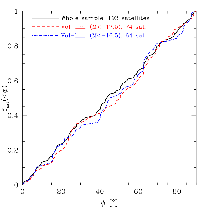
Figure 4: The cumulative distribution of the angular positions of satellites relative to their primary disk galaxies. The samples shown in this plot are the entire sample with $193$ satellites and $144$ primaries (solid line), a volume-limited subsample at a depth of $11000{\,{\mathrm{km}}\,{\mathrm{s}}^{-1}}$ with $74$ satellites and $62$ primaries (dashed line) and a volume-limited subsample at a depth of $7000{\,{\mathrm{km}}\,{\mathrm{s}}^{-1}}$ with $64$ satellites and $51$ primaries (dot-dashed line). The thin, dotted line in the background represents an isotropic cumulative distribution function.

Figure 4 shows the cumulative frequency for the entire satellite sample (solid line), compared to that of an isotropic distribution (dotted line). In addition, we computed the angular distributions of satellites in two volume-limited subsamples. The first subsample has a depth of $11000{\,{\mathrm{km}}\,{\mathrm{s}}^{-1}}$ and limiting magnitude $M_{\mathrm{B}}=-17.5$, and the second has a depth of $7000{\,{\mathrm{km}}\,{\mathrm{s}}^{-1}}$ and limiting magnitude $M_{\mathrm{B}}=-16.5$. The statistics for the volume-limited subsamples are poorer ($74$ satellites at $11000{\,{\mathrm{km}}\,{\mathrm{s}}^{-1}}$ and $64$ at $7000{\,{\mathrm{km}}\,{\mathrm{s}}^{-1}}$), but the behavior is qualitatively similar to that of the entire sample of $193$ satellites.

At first glance, this result seems most easily compatible with the simulated distribution with disk rotation nearly aligned with the angular momentum of the inner halo (Figure 2). We have performed a comparison of the distributions, using a KS test to test several hypotheses. The full observational sample as well as the volume-limited subsamples are all consistent with an isotropic distribution about their primaries. Contrary to the results of Zaritsky et al. (1997a) and Sales & Lambas (2004), this sample does not show significant evidence of anisotropy. In addition, the observed sample is consisted with all three of the hypotheses used to construct distributions from the simulation. This includes the case with the disk rotation axis aligned with the major axis of the host halo, which yields a probability $P_{\mathrm{KS}}\simeq~{}0.17$ of being drawn from the same underlying distribution. The relatively small size of the current observational sample makes it difficult to reject any of our idealized disk alignment hypotheses.

3.3 Observed Prograde Satellite Fractions

To state if a satellite is prograde or not, we need to know the difference in recessional velocity between the satellite and the primary ($\Delta v=V_{sat}-V_{prim}$), the Position Angle of the satellite with respect to the primary ($PAS$), and the sky Position Angle of the redshifted end of the primary disk ($PAred$). We define the quantity $S$ by

$$S=+1 \mathrm{if} \left\{\begin{array}[]{l}\mid PAred-PAS\mid<90^{\circ}\\ \mid PAred-PAS\mid>270^{\circ}\end{array}\right\}$$ (3)

$$S=-1 \mathrm{otherwise,}$$

A satellite is prograde if $S\cdot\Delta v>0$, and retrograde $S\cdot\Delta v<0$. Table 3 gives the sense of the line-of-sight velocities of the satellites in our sample with respect to their disk primaries.

Table 4: Prograde/Retrograde Statistics of the Entire Observational Sample

Angle from disk	$N_{\mathrm{sats}}$	$N_{\mathrm{prog}}$	$N_{\mathrm{retr}}$	$f_{\mathrm{prog}}$
$0^{\circ}$ to $+30^{\circ}$	24	15	9	$0.63\pm 0.10$
$0^{\circ}$ to $+45^{\circ}$	40	25	15	$0.63\pm 0.08$
$0^{\circ}$ to $+75^{\circ}$	58	38	20	$0.66\pm 0.06$
$0^{\circ}$ to $+90^{\circ}$	76	46	30	$0.61\pm 0.05$

Statistics of prograde/retrograde satellites for the entire sample of satellites. The columns are (1) the angular displacement from the primary disk plane, summed over the four quadrants; (2) the number of satellites for each angular selection; (3) the number of prograde satellites found for each angular selection; (4) the number of retrograde satellites found for each angular selection; (5) the frequency of prograde satellites over the total with an error estimate given by the standard deviation of the appropriate binomial distribution.

Table 5: Prograde/Retrograde Statistics for the Entire Sample to a Depth of $V<7000{\,{\mathrm{km}}\,{\mathrm{s}}^{-1}}$ (upper panel) and for a Volume-limited Sample to a Depth of $V<7000{\,{\mathrm{km}}\,{\mathrm{s}}^{-1}}$ (lower panel)

Angle from disk	$N_{\mathrm{sats}}$	$N_{\mathrm{prog}}$	$N_{\mathrm{retr}}$	$f_{\mathrm{prog}}$
$0^{\circ}$ to $+30^{\circ}$	11	8	3	$0.72\pm 0.13$
$0^{\circ}$ to $+45^{\circ}$	20	14	6	$0.70\pm 0.10$
$0^{\circ}$ to $+75^{\circ}$	34	22	12	$0.64\pm 0.08$
$0^{\circ}$ to $+90^{\circ}$	41	26	15	$0.63\pm 0.08$
Angle from disk	$N_{\mathrm{sats}}$	$N_{\mathrm{prog}}$	$N_{\mathrm{retr}}$	$f_{\mathrm{prog}}$
$0^{\circ}$ to $+30^{\circ}$	9	6	3	$0.66\pm 0.16$
$0^{\circ}$ to $+45^{\circ}$	13	8	5	$0.61\pm 0.13$
$0^{\circ}$ to $+75^{\circ}$	23	13	10	$0.57\pm 0.10$
$0^{\circ}$ to $+90^{\circ}$	28	16	12	$0.57\pm 0.09$

Prograde/Retrograde statistics of satellite galaxies for an unlimited subsample at a depth of $7000{\,{\mathrm{km}}\,{\mathrm{s}}^{-1}}$ and for a corresponding volume-limited subsample at the same depth. The depth of $7000{\,{\mathrm{km}}\,{\mathrm{s}}^{-1}}$ ($M_{\mathrm{B}}=-16.5$) has been chosen in an attempt to keep a significant number of object in each subsample. The columns are (1) the angular displacement from the primary disk plane, summed over the four quadrants; (2) the number of satellites for each angular selection; (3) the number of prograde satellites found for each angular selection; (4) the number of retrograde satellites found for each angular selection; (5) the frequency of prograde satellites over the total.

The resulting prograde satellite fractions are summarized in Table 4 and Table 5. Unfortunately, the small size of the observational sample does not allow us to study any magnitude dependence of the prograde satellite fraction at a statistically-significant level as we did for the simulated satellites in § 2.3. Alternatively, we present the prograde/retrograde fractions as a function of angular displacement from the major axis of the primary galaxy disk. Table 4 shows the resulting distribution of prograde and retrograde satellites for the entire sample at full depth ($11000{\,{\mathrm{km}}\,{\mathrm{s}}^{-1}}$). Table 5 shows two subsamples with limiting depths of $7000{\,{\mathrm{km}}\,{\mathrm{s}}^{-1}}$, one containing all objects to this depth and one for a volume-limited subsample with an absolute magnitude limit of $M_{\mathrm{B}}=-16.5$.

It is evident from Table 4 that the largest samples of satellites exhibit an excess of prograde peculiar velocities that is significant at the $\sim 2-2.5\sigma$ level. In addition, the data show no evidence for any significant trend in the prograde fraction as a function of the angular position with respect to the disk. At all angles with respect to the disk, the prograde fraction is $\sim 60\%$, though the statistical significance of the prograde excess in the smallest angular cuts is marginal. Table 5 shows a qualitatively similar result, with $f_{\mathrm{prog}}\sim 60\%$ in both of these subsamples, though again, the statistical significance is, at best, marginal in these small samples. In addition to these results we also found no significant evidence for a variation in the prograde fraction as a function of projected distance to the primary.

Figure 5 shows a histogram of the peculiar velocities of two of our samples, the entire sample with all objects and the volume-limited subsample at a depth of $7000{\,{\mathrm{km}}\,{\mathrm{s}}^{-1}}$ ($M_{\mathrm{B}}\leq-16.5$). Figure 5 shows a peak in the slowly-rotating progrades in both of these samples. This seems to be in broad agreement with the results of the simulated sample of subhalos shown in Figure 3. A more detailed analysis would require a larger observational sample.

Figure 5: The distribution of peculiar velocities of the entire unlimited sample (solid line, empty), and the volume-limited sample at a depth of $7000{\,{\mathrm{km}}\,{\mathrm{s}}^{-1}}$ (dotted line, dashed). Positive peculiar velocities correspond to prograde satellites and negative peculiar velocities correspond to retrograde satellites. The zero peculiar velocity is marked by a vertical dashed line.

4 The Effect of Observational Biases

We performed a series of Monte Carlo simulations of mock observational samples in order to quantify the effects of observational biases and interlopers. We produced lists of objects, both satellites and interlopers, distributed in magnitude according to the luminosity function of each class of object. This analysis complements the previous results on the net effect of interloper contamination in the cosmological $N$-body simulation performed in § 2.3), because it allows us to study a statistically-large number of independent, mock observations for a variety of assumptions about the true fraction of prograde satellites.

The first set of Monte Carlo simulations we performed were aimed at assessing the effect of interlopers (which are separated from their primaries by large distances along the lines of sight, but are associated due to projection) on the measured prograde/retrograde fractions of satellites relative to the prograde/retrograde fractions of “true” satellite galaxies that have small three-dimensional separations from their primaries. The number of objects at each bin of magnitude was determined using Schechter (1976) luminosity functions with different parameters according to each class of object. Specifically, we employed the magnitude form of the Schechter function,

$$\Phi(M)=0.4\Phi_{*}\log(10)\ 10^{0.4(M_{*}-M)(\alpha+1)}\exp({-10^{0.4(M_{*}-M)}}),$$ (4)

which we then used to determine the number of objects by integrating over magnitude and volume.

For the interlopers, we used the parameters given by Blanton et al. (2003) for SDSS field galaxies, converted to B band (see section 2.2), namely $\Phi_{*}=0.0074\,{\mathrm{Mpc}}^{-3}$, $M_{*}=-21.31$, $\alpha=-0.89$. In this case, the volume we considered was the same truncated cone as in our real observations, but with an additional constraint that the distance $r$ from the primary satisfies $r>1\,{h^{-1}\mathrm{Mpc}}$. This constraint serves as our working definition of “interloper” as opposed to “true” satellite.

For the satellites, we used the parameters of the Local Group (LG), assuming that it represents a typical system of satellite galaxies (Mateo, 1998; van den Bergh, 2000). The Schechter function parameters for the LG satellites were $M_{*}=-19.5$ and $\alpha=-1.14$. However, the characteristic number density $\Phi_{*}^{sat}$ for the LG is not well defined as it depends sensitively on the volume considered. A way to get a first approximation of its value is to assume a given interloper contamination, which can be taken from our Table 1 in § 2.3, and is in agreement with the fraction of interlopers found by Prada et al. (2003) from their satellite dynamics analysis. We then assume an interloper contamination of $25\%$ and calculate $\Phi_{*}^{sat}$ such that we recover $25\%$ of interloper contamination in the simulation. We used $\Phi_{*}^{sat}\simeq~{}0.07\,{\mathrm{Mpc}}^{-3}$. The volume considered for the satellites was the intersection of the truncated cone of our real observations with the sphere contained within $r<1\,{h^{-1}\mathrm{Mpc}}$ about each primary.

We then observed the objects in our simulation in the same way as we did for the SDSS data. For simplicity, in our first suite of Monte Carlo mock observations, we kept a fixed recessional velocity of $7000{\,{\mathrm{km}}\,{\mathrm{s}}^{-1}}$ for all the objects in these mock catalogs. We assumed that interlopers always have a $50\%$ chance of being prograde or retrograde, while the prograde fraction of satellites and the total number of primaries are both input parameters that are used to construct specific mock observations. The number of satellites for each galactic system (or for each primary) is then calculated using the Schechter function with the $\Phi_{*}^{sat}$ as above.

We run $500$ Monte Carlo trials, with an input prograde fraction of $f_{\mathrm{prog}}=60\%$; the input number of primary galaxies was selected such that the total number of combined false and true satellites in the mock sample was about $76$ as in our real observations. The interloper contamination in our mock samples reduced the observed prograde fraction to an average of $f_{\mathrm{prog}}=0.57$ with a root-mean-square scatter about the mean of $\pm 0.05$. This agrees quite well with the effect of interlopers found in the mock catalogs constructed from the halos in the cosmological $N$-body simulation (see Tables 1 and 2).

The second set of Monte Carlo simulations was aimed at determining how the prograde/retrograde fractions are affected by having systems at different recessional velocities mixed together, as we have in our observed sample. When several galactic systems at different recessional velocities are mixed together, different levels of interloper contamination are superposed. Also, the apparent magnitude limit of the observations results in a selection of satellite luminosities that depends on the recessional velocities of the systems. The aim is to simulate these two observational effects. We used the same setup as for the Monte Carlo simulations with fixed recessional velocities that we discussed in the previous paragraph. We built up three samples of systems, again with the necessary input number of primaries so as to “observe” a total of $76$ false and true satellites combined, at recessional velocities of $2800,5600$ and $8800{\,{\mathrm{km}}\,{\mathrm{s}}^{-1}}$. We then observed all of the samples together as a single, mock sample.

We ran a series of $500$ such random trials with an input satellite prograde fraction of $f_{\mathrm{prog}}=60\%$ as above. The mean observed percentage of prograde satellites in the mock samples was $f_{\mathrm{prog}}\simeq 58\%$, with a root-mean-square scatter of $\simeq 5\%$ about the mean. This implies that the systematic dilution of the prograde/retrograde fraction due to interlopers is fairly small for comparable samples; however, the scatter about the true fractions due to the presence of interlopers is not insignificant for samples of this size. We show in Figure 6 the mean reduction of the “observed” prograde fraction as a function of the true input prograde fraction as well as the $1\sigma$ scatter in the observed values about the mean.

Figure 6: Observed reduction of the prograde fraction caused by interloper contamination in a sample containing systems at a wide range of recessional velocities. The horizontal axis represents the true prograde fraction for all true satellites and the vertical axis represents the observed prograde fraction taking interloper contamination into account. The points represent the mean observed prograde fraction derived from our Monte Carlo simulations of the net effect of interloper contamination in the case of mixing systems with different recessional velocities. The error bars represent the root-mean-square scatter about the mean. The dotted line represents perfect retrieval of the prograde fraction.

5 Conclusions

We study the distribution of satellite galaxies about disk primaries. The study has both observational and theoretical components. We focus our attention on the fraction of satellite galaxies that exhibit prograde motion with respect to their disk primaries and on the angular distribution of satellites relative to their primaries. On the observational side, we study a carefully-selected observational sample of primary disk galaxies and satellite galaxies extracted from the Sloan Digital Sky Survey database. In addition, we analyze the structure and distribution of halos and subhalos in an $N$-body simulation of structure formation in the, now standard, concordance $\Lambda$CDM model.

We find that the fraction of prograde satellites in our entire flux-limited sample is $f_{\mathrm{prog}}=0.61\pm 0.05$. The observational samples show no evidence for a strong dependence of $f_{\mathrm{prog}}$ on magnitude, angular distance from the satellite to the major axis of the primary disk, or projected distance from the primary. However, the observed samples are, as yet, small and as a result, the statistics are poor. In addition, we found that the observed satellite galaxies are consistent with being distributed isotropically about their primary disk galaxies.

From the cosmological $N$-body simulation, we constructed catalogs of primaries and satellites using an algorithm that maps galaxies onto halos and subhalos based on matching number density (e.g. Kravtsov et al., 2004b). We built catalogs based on three idealized hypotheses for the orientations of disk galaxies within their surrounding dark matter halos, with the angular momentum of the disk aligned with either (1) the major axis of the inner host halo, (2) the minor axis of the host halo, or (3) the angular momentum of the particles in the inner host halo. We then presented the general predictions of these scenarios. The first scenario predicts a projected distribution of satellite galaxies that is strongly anisotropic, with galaxies located near the poles of their disk primaries. For example, the Kolmogorov-Smirnov probability that the entire simulated distribution of halos that are assigned magnitudes $M_{\mathrm{B}}\leq-15.5$ is selected from an underlying isotropic distribution is $P_{\mathrm{KS}}\simeq~{}5\times 10^{-5}$. However, a KS test does not yet allow us to reject this hypothesis based on the present data, largely because the observational data set is fairly small ($193$ satellites in our largest, flux-limited sample). The other two hypothesized disk orientations predict satellite distributions that are consistent with isotropy at all magnitudes. Under the hypothesis that the angular momenta of the disk primaries are aligned with the angular momenta of the inner regions of the dark matter halos that host them, the simulation predicts a prograde satellite fraction $\approx~{}55-60\%$. Specifically, for the entire sample of satellites with $M_{\mathrm{B}}\leq-15.5$, we find $f_{\mathrm{prog}}=0.54\pm 0.01$, while for a subsample of the largest satellites with $M_{\mathrm{B}}\leq-17.5$, we find $f_{\mathrm{prog}}=0.59\pm 0.03$. As the previous sentence indicates, we find that $f_{\mathrm{prog}}$ is a weak function of satellite size (magnitude), whereby larger (more luminous) satellites are more likely to exhibit prograde motions. The simulation results are broadly consistent with the values measured in the observational sample. A larger observational sample will be needed in order to test for any magnitude dependence in the observed prograde satellite fraction and to make more meaningful comparisons between theoretical predictions and observations. Larger observational samples will also require a significant refinement of theoretical predictions.

In addition to these results, we also made an effort to assess the net effect of interlopers on the observed prograde satellite fractions compared to the prograde satellite fractions for “true” satellites. From our analysis of both the $N$-body simulation and an independent set of Monte Carlo simulations of mock observations, we found that the mean dilution of the prograde satellite fraction due to interloper contamination is of the order of a few percent. However, we found that the scatter in the observed prograde and retrograde fractions in samples comparable to the size of our observational set is sizable at nearly $5\%$.

A comparable observational study including the prograde/retrograde satellite fractions and the angular distributions of satellites was performed by Zaritsky et al. (1997a, b) who had a slightly larger sample of systems. Contrary to our findings, Zaritsky et al. (1997b) reported more retrograde satellites than prograde satellites ($f_{\mathrm{prog}}\simeq 48\%$). However, note that this result is not statistically significant as an estimate of the statistical error on the mean from a sample of the size of Zaritsky et al. (1997a) gives $\sigma(f_{\mathrm{prog}})\simeq 5\%$. Zaritsky et al. (1997a) also reported strong evidence for an anisotropic satellite distribution as we mentioned in § 1. We were unable to confirm this result with our observed satellite sample, which is consistent with an isotropic underlying distribution. The nature of any disagreements between our results and the previous work of Zaritsky et al. (1997a, b) is unclear at present; however, it could possibly be due to different criteria in the selection of the objects, unaccounted for some observational biases, and/or statistical fluctuations in the relatively small samples. Larger samples constructed from forthcoming data sets should be able to address these issues as well.

References

- Afanasiev & Silchenko (1999) Afanasiev, V. L. & Silchenko, O. K. 1999, AJ, 117, 1725A
- Agustsson (2005) Agustsson, I. & Brainerd, T. G. 2005, ApJ, Submitted (astro-ph/0505272)
- Berlind & Weinberg (2002) Berlind, A. A. & Weinberg, D. H. 2002, ApJ, 575, 587
- Blanton et al. (2003) Blanton, M. R., Hogg, D. W., Bahcall, N. A., Brinkmann, J., Britton, M., Connolly, A. J., Csabai, I., Fukugita, M., Loveday, J., Meiksin, A., Munn, J. A., Nichol, R. C., Okamura, S., Quinn, T., Schneider, D. P., Shimasaku, K., Strauss, M. A., Tegmark, M., Vogeley, M. S., & Weinberg, D. H. 2003, ApJ, 592, 819
- Blumenthal et al. (1984) Blumenthal, G. R., Faber, S. M., Primack, J. R., & Rees, M. J. 1984, Nature, 311, 517
- Bond et al. (1996) Bond, J. R., Kofmann, L., & Pogosyan, D. 1996, Nature, 380, 603
- Bond & Myers (1996) Bond, J. R. & Myers, S. T. 1996, ApJS, 103, 1
- Brainerd (2004) Brainerd, T. G. 2004, ApJL, Submitted (astro-ph/0408559)
- Bryan & Norman (1998) Bryan, G. L. & Norman, M. L. 1998, ApJ, 495, 80
- Bullock (2002) Bullock, J. S. 2002, in in Proceedings of the Yale Cosmology Workshop ”The Shapes of Galaxies and Their Dark Matter Halos”, (28-30 May, 2001). P.Natarajan (ed.). Singapore: World Scientific, 109
- Carignan et al. (1997) Carignan, C., Cote, S., Freeman, K. C., & Quinn, P. J. 1997, AJ, 113, 1585
- Chen et al. (2003) Chen, D. N., Jing, Y. P., & Yoshikaw, K. 2003, ApJ, 597, 35
- Colberg et al. (2004) Colberg, J. M., Krughoff, K. S., & Connolly, A. J. 2004, MNRAS in press (astro-ph/0406665)
- Colless et al. (2001) Colless, M., Dalton, G., Maddox, S., Sutherland, W., & the 2dF collaboration. 2001, MNRAS, 328, 1039
- Diemand et al. (2004) Diemand, J., Moore, B., & Stadel, J. 2004, MNRAS, 352, 535
- Dubinski & Carlberg (1991) Dubinski, J. & Carlberg, R. G. 1991, ApJ, 378, 496
- Eke et al. (1998) Eke, V. R., Navarro, J. F., & Frenk, C. S. 1998, ApJ, 503, 569
- Fall & Efstathiou (1980) Fall, S. M. & Efstathiou, G. 1980, MNRAS, 193, 189
- Faltenbacher et al. (2005) Faltenbacher, A., Allgood, B., Gottloeber, S., Yepes, G., & Hoffman, Y. 2005, MNRAS submitted (astro-ph/0501452)
- Gao et al. (2004) Gao, L., White, S. D. M., Jenkins, A., Stoehr, F., & Springel, V. 2004, MNRAS submitted (astro-ph/0404589)
- Grebel et al. (1999) Grebel, E. K., Kolatt, T., & Brandner, W. 1999, in IAU Symposium, 447
- Hartwick (1996) Hartwick, F. D. A. 1996, in ASP Conf. Ser. 92, Formation of the Galactic Halo…Inside and Out, 444
- Hartwick (2000) Hartwick, F. D. A. 2000, AJ, 119, 2248
- Hayashi et al. (2003) Hayashi, D., Navarro, J. F., Taylor, J. E., Stadel, J., & Quinn, T. 2003, ApJ, 584, 541
- Holmberg (1969) Holmberg, E. 1969, Arkiv Astron., 5, 305
- Jenkins et al. (2001) Jenkins, A., Frenk, C. S., White, S. D. M., Colberg, J. M., Cole, S., Evrard, A. E., Couchman, H. M. P., & Yoshida, N. 2001, MNRAS, 321, 372
- Jing & Suto (2002) Jing, Y. P. & Suto, Y. 2002, ApJ, 574, 538
- Kang et al. (2005) Kang, X., Mao, S., Gao, L., & Jing, Y. P. 2005, Astron. & Astrophys. Submitted (astro-ph/0501333)
- Kazantzidis et al. (2004a) Kazantzidis, S., Kravtsov, A. V., Zentner, A. R., Allgood, B. A., Nagai, D., & Moore, B. 2004a, ApJL, 611, L73
- Kazantzidis et al. (2004b) Kazantzidis, S., Mayer, L., Mastropietro, C., Diemand, J., Stadel, J., & Moore, B. 2004b, ApJ, 608, 663
- Klypin et al. (1999) Klypin, A. A., Gottlöber, S., Kravtsov, A. V., & Khokhlov, A. M. 1999, ApJ, 516, 530
- Klypin & Shandarin (1983) Klypin, A. A. & Shandarin, S. F. 1983, MNRAS, 204, 891
- Knebe et al. (2004) Knebe, A., Gill, S. P. D., Gibson, B. K., Lewis, G. F., Ibata, R. A., & Dopita, M. A. 2004, ApJ, 603, 7
- Kravtsov (1999) Kravtsov, A. V. 1999, PhD thesis, New Mexico State University
- Kravtsov et al. (2004a) Kravtsov, A. V., Berlind, A. A., Wechsler, R. H., Klypin, A. A., Gottlöber, S., Allgood, B., & Primack, J. 2004a, ApJ, 609, 35
- Kravtsov et al. (2004b) Kravtsov, A. V., Gnedin, O. Y., & Klypin, A. A. 2004b, ApJ, 609, 482
- Kravtsov et al. (1997) Kravtsov, A. V., Klypin, A. A., & Khokhlov, A. M. 1997, ApJS, 111, 73
- Kroupa et al. (2005) Kroupa, P., Theis, C., & Boily, C. M. 2005, Astron. & Astrophys., 431, 517
- Lacey & Cole (1993) Lacey, C. & Cole, S. 1993, MNRAS, 262, 627
- Libeskind et al. (2005) Libeskind, N. I., Frenk, C. S., Cole, S., Helly, J. C., Jenkins, A., Navarro, J. F., & Power, C. 2005, MNRAS, submitted, (astro-ph/0503400)
- Lynden-Bell (1982) Lynden-Bell, D. 1982, Obs., 102, 202
- Majewski (1994) Majewski, S. R. 1994, ApJL, 431, L17
- Maller et al. (2002) Maller, A. H., Dekel, A., & Somerville, R. 2002, MNRAS, 329, 423
- Mateo (1998) Mateo, M. L. 1998, ARA&A, 36, 435
- McKay et al. (2002) McKay, T. A., Sheldon, E. S., Johnston, D., Grebel, E. K., Prada, F., Rix, H., Bahcall, N. A., Brinkmann, J., Csabai, I., Fukugita, M., Lamb, D. Q., & York, D. G. 2002, ApJ, 571, L85
- Nagai & Kravtsov (2005) Nagai, D. & Kravtsov, A. V. 2005, ApJ, 618, 557
- Peñarrubia et al. (2002) Peñarrubia, J., Kroupa, P., & Boily, C. M. 2002, MNRAS, 333, 779
- Porciani et al. (2002) Porciani, C., Dekel, A., & Hoffmann, Y. 2002, MNRAS, 332, 339
- Prada et al. (2003) Prada, F., Vitvitska, M., Klypin, A., Holtzman, J. A., Schlegel, D. J., Grebel, E. K., Rix, H.-W., Brinkmann, J., McKay, T. A., & Csabai, I. 2003, ApJ, 598, 260
- Quinn & Goodman (1986) Quinn, P. J. & Goodman, J. 1986, ApJ, 309, 472
- Sales & Lambas (2004) Sales, L. & Lambas, D. G. 2004, MNRAS, 348, 1236
- Schechter (1976) Schechter, P. 1976, ApJ, 203, 297
- Seljak (2000) Seljak, U. 2000, MNRAS, 318, 203
- Strauss et al. (2002) Strauss, M. A., Weinberg, D. H., Lupton, R. H., & the SDSS collaboration. 2002, AJ, 124, 1810
- Taffoni et al. (2003) Taffoni, G., Mayer, L., Colpi, M., & Governato, F. 2003, MNRAS, 341, 434
- Taylor & Babul (2004) Taylor, J. E. & Babul, A. 2004, MNRAS, 348, 811
- Taylor et al. (2003) Taylor, J. E., Silk, J., & Babul, A. 2003, in IAU Symp. 220: Dark Matter in Galaxies, 118
- van den Bergh (2000) van den Bergh, S., ed. 2000, The galaxies of the Local Group
- van den Bosch et al. (2002) van den Bosch, F. C., Abel, T., Croft, R. A. C., Hernquist, L., & White, S. D. M. 2002, ApJ, 576, 21
- van den Bosch et al. (2003a) van den Bosch, F. C., Mo, H. J., & Yang, X. 2003a, MNRAS, 345, 923
- van den Bosch et al. (2003b) van den Bosch, F. C., Yang, S., & Mo, H. J. 2003b, MNRAS, 340, 771
- van den Bosch et al. (2005) van den Bosch, F. C., Yang, X., Mo, H. J., & Norberg, P. 2005, MNRAS, 356, 1233
- Velázquez & White (1999) Velázquez, H. & White, S. D. M. 1999, MNRAS, 304, 254
- Vitvitska et al. (2002) Vitvitska, M., Klypin, A. A., Kravtsov, A. V., Wechsler, R. H., Primack, J. R., & Bullock, J. S. 2002, ApJ, 581, 799
- Warren et al. (1992) Warren, M. S., Quinn, P. J., Salmon, J. K., & Zurek, W. H. 1992, ApJ, 340, 771
- White & Rees (1978) White, S. D. M. & Rees, M. J. 1978, MNRAS, 183, 341
- Willman et al. (2004) Willman, B., Governato, F., Dalcanton, J. J., Reed, D., & Quinn, T. 2004, MNRAS, 353, 639
- Yang et al. (2003) Yang, X., Mo, H. J., & van den Bosch, F. C. 2003, MNRAS, 339, 1057
- York et al. (2000) York, D. G., Adelman, J., Anderson, J. E., Anderson, S. F., Annis, J., & the SDSS collaboration. 2000, AJ, 120, 1579
- Zaritsky & Gonzalez (1999) Zaritsky, D. & Gonzalez, A. H. 1999, PASP, 111, 1508
- Zaritsky et al. (1997a) Zaritsky, D., Smith, R., Frenk, C. S., & White, S. D. M. 1997a, ApJL, 478, L53
- Zaritsky et al. (1997b) Zaritsky, D., Smith, R., Frenk, C. S., & White, S. D. M. 1997b, ApJ, 478, 39
- Zentner et al. (2005a) Zentner, A. R., Berlind, A. A., Bullock, J. S., Kravtsov, A. V., & Wechsler, R. H. 2005a, ApJ, 624, 505
- Zentner & Bullock (2003) Zentner, A. R. & Bullock, J. S. 2003, ApJ, 598, 49
- Zentner et al. (2005b) Zentner, A. R., Kravtsov, A. V., Gnedin, O. Y., & Klypin, A. A. 2005b, ApJ, In Press, 629 (astro-ph/0502496)
- Zheng et al. (2004) Zheng, Z., Berlind, A. A., Weinberg, D. H., Benson, A. J., Baugh, C. M., Cole, S., Davé, R., Frenk, C. S., Katz, N., & Lacey, C. G. 2004, ApJ, Submitted, (astro-ph/0408569)