Dynamical insight into dark-matter haloes

Abstract

We investigate, using the spherical Jeans equation, self-gravitating dynamical equilibria satisfying a relation $\rho/\sigma_{r}^{3}\propto r^{-\alpha}$, which holds for simulated dark-matter haloes over their whole resolved radial range. Considering first the case of velocity isotropy, we find that this problem has only one solution for which the density profile is not truncated or otherwise unrealistic. This solution occurs only for a critical value of $\alpha_{\mathrm{crit}}=35/18=1.9\overline{4}$, which is consistent with the empirical value of $1.9\pm 0.05$. We extend our analysis in two ways: first we introduce a parameter $\epsilon$ to allow for a more general relation $\rho/\sigma_{r}^{\epsilon}\propto r^{-\alpha}$; second we consider velocity anisotropy parameterised by Binney’s $\beta(r)\equiv 1-\sigma_{\theta}^{2}/\sigma_{r}^{2}$. If we assume $\beta$ to be linearly related to the logarithmic density slope $\gamma(r)\equiv-\mathrm{d}\ln\rho/\mathrm{d}\ln r$, which is in agreement with simulations, the problem remains analytically tractable and is equivalent to the simpler isotropic case: there exists only one physical solution, which occurs at a critical $\alpha$ value. Remarkably, this value of $\alpha$ and the density and velocity-dispersion profiles depend only on $\epsilon$ and the value $\beta_{0}\equiv\beta(r=0)$, but not on the value $\beta_{\infty}\equiv\beta(r\to\infty)$ (or, equivalently, the slope $\mathrm{d}\beta/\mathrm{d}\gamma$ of the adopted linear $\beta$-$\gamma$ relation). For $\epsilon=3$, $\alpha_{\mathrm{crit}}=35/18-2\beta_{0}/9$ and the resulting density profile is fully analytic (as are the velocity dispersion and circular speed) with an inner cusp $\rho\propto r^{-(7+10\beta_{0})/9}$ and a very smooth transition to a steeper outer power-law asymptote. These models are in excellent agreement with the density, velocity-dispersion and anisotropy profiles of simulated dark-matter haloes over their full resolved radial range. If $\epsilon=3$ is a universal constant, some scatter in $\beta_{0}\approx 0$ may account for some diversity in the density profiles, provided a relation $\rho/\sigma_{r}^{3}\propto r^{-\alpha_{\mathrm{crit}}}$ always holds.

1 Introduction

It has long been recognised that $N$-body studies of large-scale structure formation in cold dark matter (CDM) cosmologies produce dark-matter haloes whose density profiles are remarkably similar in shape over a wide range of halo virial mass (e.g. Dubinski & Carlberg, 1991; Crone et al., 1994; Navarro et al., 1996, 1997; Moore et al., 1999; Bullock et al., 2001). This ‘universal’ halo density distribution is characterised by a relatively shallow power-law behaviour in the inner parts, $\rho\sim r^{-\gamma}$, with $\gamma\approx 1$ typically inferred at the smallest resolved radii, which steepens gradually to an extrapolated $\gamma\approx 3-4$ at arbitrarily large radii.

A physical explanation, based on first principles, for the origin of such a profile is still lacking, and there has been some considerable debate over the exact functional form implied by the numerical studies. The fitting function most commonly applied has the general form

$$\rho(r)\propto r^{-\gamma_{0}}(r_{s}+r)^{\gamma_{0}-\gamma_{\infty}},$$ (1)

where $\gamma_{0}$ and $\gamma_{\infty}$ are the power-law slopes of the central cusp and in the limit $r\to\infty$, respectively, while $r_{s}$ is an appropriate scale radius. Dubinski & Carlberg (1991) originally suggested the Hernquist (1990) profile, corresponding to $\gamma_{0}=1$ and $\gamma_{\infty}=4$, while Navarro, Frenk & White (1996, 1997) argued for $\gamma_{0}=1$ but $\gamma_{\infty}=3$ (the so-called ‘NFW’ profile). Subsequently, several studies have argued for a somewhat steeper central cusp (e.g. Moore et al., 1998, 1999; Ghigna et al., 1998, 2000; Fukushige & Makino, 1997, 2001), with one recent suite of high-resolution simulations appearing to imply $\gamma_{0}\simeq 1.16\pm 0.14$ (Diemand et al., 2004b). However, even the highest-resolution simulation to date (Diemand et al., 2005, $\gamma_{0}=1.2$) can resolve the halo structure only to a fraction $10^{-3}$ of its virial radius, and this for a single halo only. Much more common are numerical resolution limits several times larger than that, leaving room for the possibility that halo densities might become shallower than $r^{-1}$ at very small (‘unobserved’) radii (Taylor & Navarro, 2001; Power et al., 2003; Fukushige et al., 2004; Hayashi et al., 2004), and perhaps even tend to a finite density at $r=0$ with no cusp at all (Stoehr et al., 2002; Navarro et al., 2004; Merritt et al., 2005). Alternatively, there might be no single, ‘universal’ density slope in this limit (Navarro et al., 2004; Fukushige et al., 2004). At the other extreme, there are very few hard constraints on any limiting value of the density slope as $r\to\infty$, as any halo is only well defined within a finite virial radius.

    

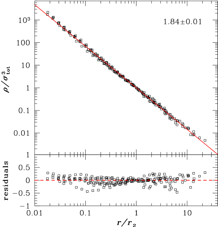
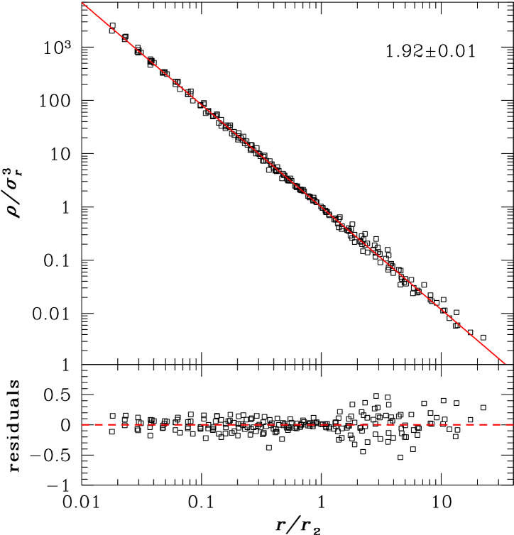
Figure 1: Plots of $\rho/\sigma_{\mathrm{tot}}^{3}$ (left) and $\rho/\sigma_{r}^{3}$ (right) as functions of radius for ten simulated CDM haloes from Diemand et al. (2004a, b), namely the six cluster-sized haloes called A9, B9, C9, D12, E9, and F9 and the four galaxy-sized haloes G0, G1, G2, and G3. The radial coordinate in each halo has been scaled by the radius $r_{2}$ at which $\mathrm{d}\ln\rho/\mathrm{d}\ln r=-2$ for that halo, and both ratios $\rho/\sigma_{\mathrm{tot}}^{3}$ and $\rho/\sigma_{r}^{3}$ have been normalised by their respective values at $r_{2}$. The lines in the upper panels are power-law fits to the scaled data from all ten haloes combined. The average negative slope and its uncertainty are indicated. In the bottom panels, we show the relative residuals $[(\rho/\sigma^{3})-(\rho/\sigma^{3})_{\mathrm{fit}}]/(\rho/\sigma^{3})$. The rms residual is essentially the same ($0.14$–$0.15$) whether $\sigma_{\mathrm{tot}}$ or $\sigma_{r}$ is involved, although in the latter case they are arguably distributed more uniformly about 0.

In this paper, we examine the question of dark-matter halo structure from a slightly different viewpoint, opting to derive $\rho(r)$ from a simple dynamical Ansatz, rather than fitting a pre-set family of functions to simulated density profiles. Our starting point is still empirical, however, being based on another surprisingly uniform property of $N$-body haloes. As was first noted and exploited by Taylor & Navarro (2001), the ratio of the density $\rho(r)$ and the cube of the velocity dispersion $\sigma(r)$ is a single power-law in radius

$$\rho(r)/\sigma(r)^{3}\propto r^{-\alpha}$$ (2)

over the full numerically resolved radial range. Taylor & Navarro originally found $\alpha=15/8=1.875$, which interestingly is the value predicted by the classic similarity solution for spherical secondary infall (Bertschinger, 1985). They then used this constraint to solve the Jeans equation numerically (assuming an isotropic velocity distribution) for $\rho(r)$ and $\sigma(r)$ separately. Although their result for $\rho(r)$ is not of the form (1) (it does tend to a shallow power law at the centre but steepens rapidly outwards and falls to zero at a finite radius), Taylor & Navarro argued such a density distribution to be an adequate description of simulation data inside the virial radius. Unfortunately, there is no exact analytical expression for $\rho(r)$ in the case $\alpha=1.875$, and this approach has not been used for fitting any data. Other studies have subsequently confirmed that $\rho/\sigma^{3}$ is a power law in radius, but estimates of the exponent differ somewhat from the Taylor-Navarro value: $\alpha=1.95$ or $1.90\pm 0.05$ according to Rasia, Tormen & Moscardini (2004) and Ascasibar et al. (2004), respectively.

Our main aim is to investigate in more detail the structure and dynamics of spherical dark-matter haloes that follow a ‘$\rho$-$\sigma$ relation’ of the basic type given in equation (2), allowing at least initially for arbitrary values of $\alpha$. Thus, in Figure 1 we show this relation as defined by ten CDM haloes simulated by Diemand, Moore & Stadel (2004a, b), the details of which were kindly provided to us by Jürg Diemand. These include four galaxy-sized haloes and six cluster-sized haloes, with virial masses ranging from $10^{12}\,M_{\odot}$ to $10^{15}\,M_{\odot}$. All are dynamically relaxed. The left panels of Fig. 1 examine the ratio $\rho/\sigma_{\mathrm{tot}}^{3}$ as a function of radius in these haloes, where the total one-dimensional velocity dispersion is $\sigma_{\mathrm{tot}}^{2}\equiv\frac{1}{3}(\sigma_{r}^{2}+\sigma_{\theta}^{2}+\sigma_{\phi}^{2})$. The right panels look at the quantity $\rho/\sigma_{r}^{3}$ vs. $r$, where $\sigma_{r}$ is the velocity dispersion in the radial direction only. Power-law fits to each of these profiles are drawn, and the residuals from the fits are shown in the bottom panels. These demonstrate that the ratio $\rho/\sigma_{r}^{3}$ follows a power law in radius at least as closely as $\rho/\sigma_{\mathrm{tot}}^{3}$ does, although the fitted slopes differ slightly between the two cases. Fits for each of the ten haloes individually yield power-law slopes that can differ by $\pm 4\%$ from the average values in Fig. 1. Whether this scatter is real or simply a reflection of numerical uncertainties is unclear, but it is certainly rather modest.

To the extent that either of the $\rho$-$\sigma$ relations illustrated in Fig. 1 is ‘universal’, and insofar as dark-matter haloes are in equilibrium, imposing a dynamical constraint along the lines of equation (2) to solve the spherical Jeans equation, as Taylor & Navarro originally did, should lead directly to a ‘universal’ density profile. While we have no physical argument for the fundamental origin of the precise power-law behaviour in Figure 1 (though clearly it must be related to the initial conditions and the formation via violent relaxation), it is much simpler to characterise than the density profile itself. Moreover, a Jeans-equation approach allows explicitly for a simultaneous exploration of velocity anisotropy inside haloes—an issue which to date has been largely divorced from empirical descriptions of the halo density profiles.

It is well known that the velocity distributions in dark-matter haloes are not isotropic. We characterise velocity anisotropy using Binney’s parameter

$$\beta(r)=1-\frac{\sigma_{\theta}^{2}+\sigma_{\phi}^{2}}{2\sigma_{r}^{2}},$$ (3)

such that $0<\beta\leq 1$ corresponds to radial anisotropy and $\beta<0$ signifies a tangentially biased velocity distribution. It is typically found that $\beta\approx 0$ (isotropy) at the centres of haloes and gradually increases outwards (reflecting radial anisotropy), reaching levels of $\beta\approx 0.5$ around the virial radius (e.g., Colín et al., 2000; Fukushige & Makino, 2001). Indeed, it has been suggested (Cole & Lacey, 1996; Carlberg et al., 1997) that there exists a ‘universal’ anisotropy profile in dark-matter haloes. Very closely related to such an idea is the recent claim by Hansen & Moore (2005), that $\beta(r)$ depends roughly linearly on the logarithmic density gradient

$$\gamma(r)\equiv-\mathrm{d}\ln\rho/\mathrm{d}\ln r$$ (4)

with essentially the same, constant slope $\mathrm{d}\beta/\mathrm{d}\gamma$ holding for a variety of end-products of violent relaxation processes (merger remnants, dark-matter haloes, collapse remnants).

With these points particularly in mind, we base our analysis on the assumption that halo density and the radial component of velocity dispersion $\sigma_{r}$ (rather than $\sigma_{\mathrm{tot}}$) are connected through a power-law relation of the general form

$$\frac{\rho}{\sigma_{r}^{\epsilon}}(r)=\frac{\rho_{0}}{\sigma_{r,0}^{\epsilon}}\,\left(\frac{r}{r_{0}}\right)^{-\alpha},$$ (5)

where $r_{0}$ is any convenient reference radius, $\rho_{0}=\rho(r_{0})$, and $\sigma_{r,0}=\sigma_{r}(r_{0})$. Intuitively, as well as on the basis of Figure 1, it seems most natural to expect the exponent $\epsilon$ in this equation to be $\epsilon=3$; but it adds little complication to allow for the possibility (Hansen, 2004) that a slightly different value might provide a still more accurate description of simulated haloes. The choice of $\sigma_{r}$ as the velocity dispersion to work with is arguably more natural than $\sigma_{\mathrm{tot}}$, since $\beta(r)$ and $\sigma_{r}$ appear separately in the spherical Jeans equation but $\sigma_{\mathrm{tot}}^{2}=\sigma_{r}^{2}(1-2\beta/3)$. Technically, this choice ultimately allows for a more tractable inclusion of velocity anisotropy; empirically, it is obviously well justified by Figure 1.

We begin in Section 2 with an investigation into which spherical density profiles satisfy the Jeans equation and obey the Ansatz (5) under the restrictions of velocity isotropy ($\beta\equiv 0$ and $\sigma_{\mathrm{tot}}\equiv\sigma_{r}$) and a fixed $\epsilon=3$. The problem is then identical to the one first considered by Taylor & Navarro (2001), and our approach is rooted in theirs, but we also draw on some aspects of the considerations by Williams et al. (2004). However, unlike these authors, we explore the full solution space of the problem. We find that only very few of the many possible solutions correspond to realistic density models for simulated dark-matter haloes, and in fact only one solution, which occurs for a ‘critical’ value of $\alpha$, is of practical importance.

We then proceed in Section 3 to consider the more realistic case of anisotropic velocity distributions and allow for general values of $\epsilon$ in equation (5). We show that in the case of an anisotropy parameter $\beta$ that depends linearly on $\gamma$ (including constant anisotropy as a special case), and for any $\epsilon$, the solutions of the Jeans equation under our adopted constraint are exact analogues of those in the $\beta\equiv 0$, $\epsilon=3$ case. In particular, for each pair ($\epsilon$, $\beta(r=0)$) only one physical solution of practical relevance exists, which again occurs at a ‘critical’ $\alpha$ value. These solutions have fully analytical density, mass, and velocity-dispersion profiles with power-law asymptotes at small and large radii.

In Section 4 we compare our analytical profiles to the ‘observed’ density, velocity dispersion, and anisotropy profiles in haloes simulated by Diemand et al. (2004a, b); Diemand et al. (2005), finding good agreement in general. Finally, Section 5 discusses our findings and summarises the paper.

2 The isotropic case

Our underlying assumption is that some version of the general $\rho$-$\sigma$ relation in equation (5) holds for dark-matter haloes. Before allowing for this level of generality, however, there is much insight to be gained from beginning with a more specialised case, in which the velocity distribution is isotropic and $\epsilon=3$. Then, as in Taylor & Navarro (2001), Williams et al. (2004), and Hansen (2004), we have

$$\frac{\rho}{\sigma_{r}^{3}}=\frac{\rho_{0}}{\sigma_{r,0}^{3}}\,\left(\frac{r}{r_{0}}\right)^{-\alpha}.$$ (6)

The Jeans equation for a spherical, self-gravitating collisionless system with isotropic velocity distribution is

$$\frac{\mathrm{d}(\rho\sigma_{r}^{2})}{\mathrm{d}r}=-\rho(r)\,\frac{GM(r)}{r^{2}}$$ (7)

with $M(r)=4\pi\int_{0}^{r}u^{2}\rho(u)\,\mathrm{d}u$. Following Taylor & Navarro, we solve equation (6) for $\sigma_{r}$, insert it in equation (7), and differentiate again to obtain

$$\frac{1}{x^{2}y}\frac{\mathrm{d}}{\mathrm{d}x}\left[\frac{x^{2}}{y}\frac{\mathrm{d}}{\mathrm{d}x}(y^{5/3}x^{2\alpha/3})\right]=-\kappa.$$ (8)

Here, $x\equiv r/r_{0}$ and $y\equiv\rho/\rho_{0}$ are dimensionless variables, and

$$\kappa\equiv 4\pi G\rho_{0}r_{0}^{2}/\sigma_{r,0}^{2}$$ (9)

is a dimensionless measure of the velocity dispersion scale. Taylor & Navarro studied the solutions of equation (8) for the particular value $\alpha=15/8$ by numerical integration. It proves useful, however, to first re-write the problem in terms of the (negative) logarithmic density slope $\gamma(r)$, as defined in (4). Equation (8) then reads

$$\gamma^{\prime}-\tfrac{2}{3}(\gamma-\gamma_{a})\,(\gamma-\gamma_{b})=\tfrac{3}{5}\kappa x^{2-2\alpha/3}y^{1/3},$$ (10)

where a prime denotes differentiation with respect to $\ln x$ and

$$\gamma_{a}=\tfrac{2}{5}\,\alpha,\qquad\gamma_{b}=\alpha+\tfrac{3}{2}.$$ (11)

The objective of this Section is to investigate the solution space of equation (10). First, note that its r.h.s. becomes constant for $y=x^{-\gamma_{1}}$, with

$$\gamma_{1}=6-2\alpha.$$ (12)

In fact, as was already noted by Taylor & Navarro, this singular density profile is a solution to equation (10) and, for $\alpha=2$ corresponds to the well-known singular isothermal sphere. For $3/2<\alpha<5/2$ (which covers our regime of interest; see Figure 1 above),

$$\gamma_{a}<\gamma_{1}<\gamma_{b}$$ (13)

and thus, following Taylor & Navarro, we choose to identify the reference radius $r_{0}$ in equation (6) as that at which the (negative) density slope equals $\gamma_{1}$, i.e., $\gamma_{1}=\gamma(x=1)$. In this way, $r_{0}$ is well-defined for all realistic solutions. Moreover, it is then obvious from this equation that the constant $\kappa$ is effectively a measure of $\gamma^{\prime}$ at $x=1$.

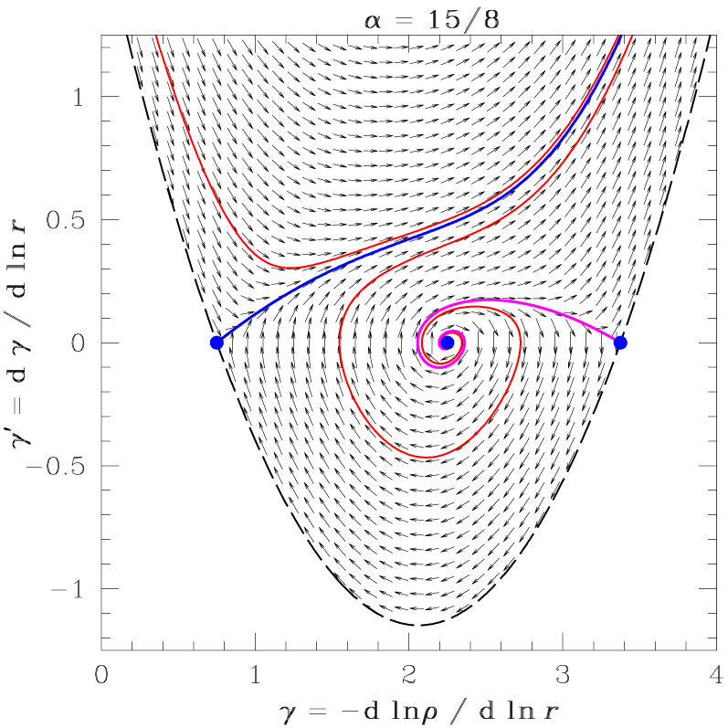
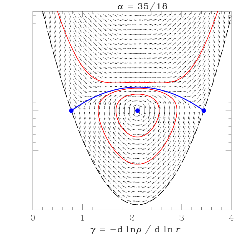
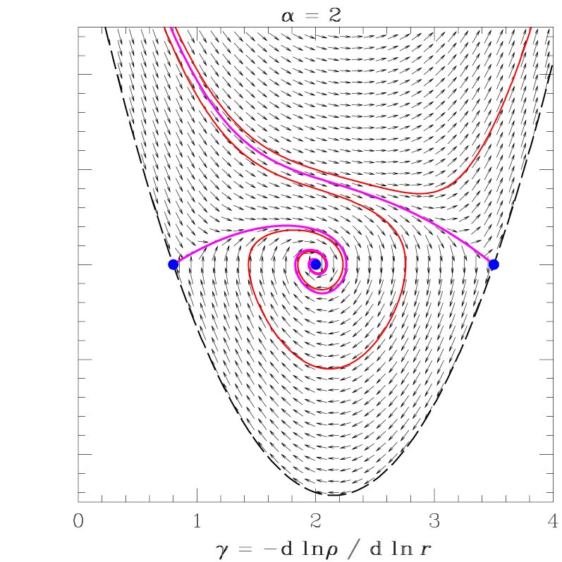
Figure 2: Flow diagrams of equation (14), describing isotropic density profiles with $\rho/\sigma_{r}^{3}\propto r^{-\alpha}$, in the $(\gamma,\gamma^{\prime})$ phase space (the length of the arrows has been normalised for ease of reading) for three different values of $\alpha$. The flow vanishes at the three fixed points (dots), where $\gamma^{\prime}=0$ and $\gamma$ is a root of the right-hand side of equation (14). Some solutions to equation (14) are given as curves. Physical solutions to the original equation (10) must lie above the (dashed) parabola, which is defined in equation (15). Solutions with $\gamma^{\prime}<0$ or $\gamma<0$ at any point (red and magenta curves) are unrealistic. There is exactly one realistic and physical solution for every $\alpha\leq 35/18$ (blue curve) and none for larger $\alpha$. At small radii this solution’s density profile approaches the power-law $\rho\propto r^{-2\alpha/5}$, while at large radii the density is truncated at a finite radius for $\alpha<35/18$, and approaches $\rho\propto r^{-\alpha-3/2}=r^{-31/9}$ for $\alpha=35/18$.

Let us now consider equation (10) in some detail, in particular the possible behaviour of any solutions at very small and large radii (see also Williams et al.). It is straightforward to verify that in the limit $r\to 0$ only three asymptotes are possible: either $\gamma\to\gamma_{a}$ (both sides of the equation vanish, so long as $\alpha<5/2$); or $\gamma\to\gamma_{1}$ (both sides approach a constant); or the density has a central hole with $y\equiv 0$ inside a non-zero radius (note that $\gamma\to\gamma_{b}$ is not possible, since the r.h.s. would then diverge for $\alpha>3/2$). Of these three, the latter is unrealistic, whereas $\gamma\to\gamma_{1}$ is inconsistent with simulated haloes, which have shallower inner density slopes. This leaves $\gamma\to\gamma_{a}$ as the only interesting option. We thus expect that, for any given value of $\alpha$, there exists one solution with $\gamma\to\gamma_{a}$ as $r\to 0$. The solution with this limiting behaviour is associated with a unique value of $\kappa$, which depends on $\alpha$ through equation (10). In fact, this very case corresponds to the ‘critical $\kappa$’ solution developed by Taylor & Navarro for their specified $\alpha=15/8$.

In the limit $r\to\infty$, also only three possible asymptotes exist: either $\gamma\to\gamma_{b}$ (both sides of the equation vanish, if $\alpha>3/2$), or $\gamma\to\gamma_{1}$ (both sides approach a constant again), or the density has an outer truncation with $y\equiv 0$ beyond a finite radius (note that $\gamma\to\gamma_{a}$ is not possible, as the r.h.s. then diverges if $\alpha<5/2$). All of these three are physically meaningful (apart from the fact that for $\gamma\to\gamma_{1}$ the mass formally diverges, similarly to the isothermal sphere). Taylor & Navarro’s ‘critical $\kappa$’ solution for $\alpha=15/8$ is one with an outer truncation.

In order to gain more insight into the solution space of equation (10), we now follow Williams et al. and differentiate it yet again (with respect to $\ln x$) to obtain

$$\gamma^{\prime\prime}-\gamma^{\prime}\,\Big{(}\gamma-\tfrac{1}{3}[2\gamma_{a}+2\gamma_{b}-\gamma_{1}]\Big{)}=\tfrac{2}{9}(\gamma-\gamma_{a})\,(\gamma-\gamma_{b})\,(\gamma-\gamma_{1}),$$ (14)

equivalent to their equation (2.2). In Figure 2, we plot flow diagrams of the $(\gamma,\gamma^{\prime})$ phase space for three representative values of $\alpha$. The dashed parabola in each panel corresponds to

$$\gamma^{\prime}=\gamma^{\prime}_{\mathrm{min}}\equiv\tfrac{2}{3}(\gamma-\gamma_{a})\,(\gamma-\gamma_{b}).$$ (15)

While this actually is a solution to (14), as already discovered by Williams et al., it is not a valid solution to the original, physical problem. This is because the constant $\kappa>0$ by definition, so equation (10) requires that $\gamma^{\prime}\geq\gamma^{\prime}_{\mathrm{min}}$ in order for its r.h.s. to be non-negative. In fact, the equality $\gamma^{\prime}=\gamma^{\prime}_{\mathrm{min}}$ is only allowed in either of the limits $\gamma\to\gamma_{a}$ as $r\to 0$ or $\gamma\to\gamma_{b}$ as $r\to\infty$ (see the discussion above). Similarly, any solutions below the parabola (15) require $\kappa<0$ and are unphysical. By contrast, all solutions above the parabola (15) correspond to potentially viable solutions of the original equation (10).

In all panels of Figure 2, the flow vanishes at the three fixed points $(\gamma,\gamma^{\prime})=(\gamma_{a},0)$, $(\gamma_{1},0)$, and $(\gamma_{b},0)$, which are plotted as blue dots. The central fixed point is stable and corresponds to the singular solution $y=x^{-\gamma_{1}}$ discussed above. Solutions with $\gamma^{\prime\prime}>0$ (arrows pointing upwards) at any $\gamma>\gamma_{1}$ approach, in the limit $\gamma\to\infty$, the upper right branch of the parabola $\gamma^{\prime}=\gamma^{\prime}_{\mathrm{min}}$. This corresponds to the case, discussed above, of an outer truncation to the density. More precisely, integrating equation (15) twice yields the asymptotic density profile

$$\rho\to r^{-\gamma_{b}}\big{(}r_{t}^{2(\gamma_{b}-\gamma_{a})/3}-r^{2(\gamma_{b}-\gamma_{a})/3}\big{)}^{3/2}$$ (16)

as $r$ approaches some finite radius $r_{t}$. For $r\geq r_{t}$, $\rho\equiv 0$. Conversely, solutions with $\gamma^{\prime\prime}<0$ (arrows pointing downwards) at any $\gamma<\gamma_{1}$ approach, in the limit $\gamma\to-\infty$, the upper left branch of the parabola. This corresponds to the case, mentioned above, of an inner truncation, with the asymptotic density profile

$$\rho\to r^{-\gamma_{a}}\big{(}r_{h}^{2(\gamma_{a}-\gamma_{b})/3}-r^{2(\gamma_{a}-\gamma_{b})/3}\big{)}^{3/2}$$ (17)

as $r$ approaches some radius $r_{h}>0$. For $r\leq r_{h}$, $\rho\equiv 0$. Thus solutions for which $\gamma\to\infty$ at large radii have a finite outer truncation radius, and solutions for which $\gamma\to-\infty$ at small radii have a finite-sized inner hole. These latter solutions are clearly unrealistic and also unphysical (the isotropic distribution function must become negative to account for the hole). Furthermore, solutions that ever visit $\gamma^{\prime}<0$ are hardly realistic (their density profiles become shallower towards larger radii, at least over some radial range).

Apart from this—as Williams et al. (2004) have also noted—the generic behaviour of the solutions to equation (14) depends on whether $\alpha$ is greater than, less than, or equal to a critical value $\alpha_{\mathrm{crit}}$ for which the inner and outer fixed points $\gamma_{a}$ and $\gamma_{b}$ are equidistant from the central $\gamma_{1}$. Referring to equations (11) and (12), $\gamma_{1}=\tfrac{1}{2}(\gamma_{a}+\gamma_{b})$ requires $\alpha_{\mathrm{crit}}=35/18=1.9\overline{4}$.

The behaviour of the solutions for $\alpha>\alpha_{\mathrm{crit}}$ is exemplified in the right panel of Fig. 2. The solutions are split into two families by the one (upper magenta) which ends at the fixed point at $\gamma=\gamma_{b}$, so that $\rho\propto r^{-\gamma_{b}}$ as $r\to\infty$. Solutions lying above this curve correspond to density profiles with a central hole and an outer truncation; those below usually also have a central hole but at larger radii perform damped ‘oscillations’ about $\gamma=\gamma_{1}$, eventually approaching $\rho\propto r^{-\gamma_{1}}$ as $r\to\infty$. All of these solutions are unrealistic, since they possess inner density holes. The only exception is a limiting solution (lower magenta) which starts from the fixed point at $\gamma=\gamma_{a}$ (i.e., $\rho\propto r^{-\gamma_{a}}$ as $r\to 0$) and slowly approaches $\gamma=\gamma_{1}$ as $r\to\infty$. However, this solution is still not a viable description of dark-matter haloes, since its density profile is too shallow at large radii.

The behaviour of the solutions when $\alpha<\alpha_{\mathrm{crit}}$ is illustrated in the left panel of Fig. 2 for $\alpha=15/8$, the case previously studied by Taylor & Navarro. The situation is in some sense a mirrored version of that for $\alpha>\alpha_{\mathrm{crit}}$. The solution space is again divided into two families, now by the solution (blue) starting from the left fixed point at $\gamma=\gamma_{a}$ at $r=0$. Solutions above this one again correspond to density profiles with a central hole and an outer truncation; those below it start from an ‘oscillation’ about the power-law $\rho\propto r^{-\gamma_{1}}$ in the limit $r\to 0$, eventually steepening outwards and generally being truncated at a finite large radius. The limit of this family is the solution (magenta) which instead of an outer truncation has a power-law fall-off with $\rho\propto r^{-\gamma_{b}}$ as $r\to\infty$.

For any $\alpha<\alpha_{\mathrm{crit}}$, the (blue) solution separating the two families just described is a potentially realistic model for dark-matter haloes, starting as it does from a shallow power-law cusp $\rho\propto r^{-\gamma_{a}}$ at $r\to 0$ (with $\gamma_{a}=2\alpha/5<7/9$ for $\alpha<35/18$) and steepening outwards to reach $\rho=0$ at a finite radius. This is the model identified by Taylor & Navarro as their ‘critical $\kappa$’ solution in the specific case $\alpha=15/8$. Given this $\alpha$, numerical integration of equation (14) outwards from $\gamma=\gamma_{a}=3/4$ at $x=0$ yields $\kappa=2.674$, to be compared with the value $\kappa=2.678$ found by Taylor & Navarro through trial-and-error integration of equation (8) starting from $x=1$.

The middle panel of Figure 2 depicts the special situation $\alpha=\alpha_{\mathrm{crit}}$, for which the flow in $(\gamma,\gamma^{\prime})$ phase-space is symmetric with respect to the transformation $r\to r^{-1}$ and $\gamma\to 2\gamma_{1}-\gamma$ (because $\gamma_{a}+\gamma_{b}=2\gamma_{1}$ by definition of $\alpha_{\mathrm{crit}}$) In this case, there exists a first integral,

$$K=\Big{(}\gamma^{\prime}+\tfrac{1}{6}(\gamma-\gamma_{a})(\gamma-\gamma_{b})\Big{)}\,\Big{(}\gamma^{\prime}-\tfrac{2}{3}(\gamma-\gamma_{a})(\gamma-\gamma_{b})\Big{)}^{4}\ ,$$ (18)

which is conserved by any solution of equation (14) with $\alpha=\alpha_{\mathrm{crit}}$. In particular, $K=0$ for the solution $\gamma^{\prime}=\gamma^{\prime}_{\mathrm{min}}(\gamma)$ (see eq. [15]) and also for

$$\gamma^{\prime}=-\tfrac{1}{6}(\gamma-\gamma_{a})(\gamma-\gamma_{b})$$ (19)

which is plotted as the blue curve in the middle panel of Figure 2. It again divides the solution space into two, although now solutions above the curve (19) always have both an inner hole and an outer truncation to the density profile, while solutions below the curve undergo undamped ‘oscillations’ about $\rho\propto r^{-\gamma_{1}}$, never settling to an asymptote in either limit $r\to 0$ or $r\to\infty$.

The solution (19) for $\alpha=\alpha_{\mathrm{crit}}=35/18$ is particularly appealing since it starts from a shallow power law $\gamma\to\gamma_{a}=7/9$ in the limit $r\to 0$ and tends to the steeper $\gamma\to\gamma_{b}=31/9$ as $r\to\infty$. The combination of these features is reminiscent of dark-matter haloes. This single solution with $\alpha=\alpha_{\mathrm{crit}}$ is the only one, of all the solutions for any $\alpha$, whose density has both inner and outer power-law asymptotes and monotonically increasing $\gamma$. It is also the only one we have found which is simple enough that almost all its physical properties can be developed analytically: equation (19) is easily integrated to give $\gamma(x)$ and subsequently $y(x)\propto\rho(r)$ as simple functions, which then allows us to evaluate $\sigma_{r}(r)$, the enclosed mass profile $M(r)$, and the circular velocity $V_{c}(r)$.

To aid in obtaining these basic results, we first substitute equation (19) into equation (10) and evaluate the result at $x=y=1$ (where $\gamma=\gamma_{1}$ by definition) to find

$$\kappa=\tfrac{25}{18}(\gamma_{1}-\gamma_{a})(\gamma_{b}-\gamma_{1})=\tfrac{200}{81}$$ (20a)

(for $$\alpha=\alpha_{\mathrm{crit}}$$). With this in hand, we obtain

$$\rho(r) = \frac{5}{9}\frac{M_{\mathrm{tot}}}{\pi r_{0}^{3}}x^{-7/9}\Big{(}1+x^{4/9}\Big{)}^{-6},$$ (20b)

$$\gamma(r) = \frac{\tfrac{7}{9}+\tfrac{31}{9}x^{4/9}}{1+x^{4/9}},$$ (20c)

$$\sigma_{r}^{2}(r) = \frac{9}{40}\frac{GM_{\mathrm{tot}}}{r_{0}}x^{-1}\left(\frac{x^{4/9}}{1+x^{4/9}}\right)^{4},$$ (20d)

$$M(r) = M_{\mathrm{tot}}\left(\frac{x^{4/9}}{1+x^{4/9}}\right)^{5},$$ (20e)

$$V_{c}^{2}(r) = \frac{GM_{\mathrm{tot}}}{r_{0}}x^{-1}\left(\frac{x^{4/9}}{1+x^{4/9}}\right)^{5},$$ (20f)

where $$x\equiv r/r_{0} \rho_{0} M_{\mathrm{tot}}=(576\pi/5)\,\rho_{0}r_{0}^{3} \kappa \sigma_{r,0} \sigma_{r}^{2}(r) V_{c}^{2}(r) r^{-1} r\to\infty r=0 x=(7/9)^{9/4} \sigma_{r}^{2}(r) x=(11/9)^{9/4} V_{c}^{2}(r) \mathrm{d}\Phi/\mathrm{d}r=GM(r)/r^{2}$$ as usual. We have replaced with the total mass ; and the value of in equation (20a) has been used with the basic definition (9) to eliminate the normalisation from equation (20d). Note that, because this solution has a finite total mass, both and fall off as in the limit . At the same time, both quantities vanish at , and thus each profile peaks at a finite radius. This happens at for , and at for . Finally, the gravitational potential follows from integrating :

$$\Phi(r)=-\frac{9}{4}\frac{G\,M_{\mathrm{tot}}}{r_{0}}B_{\frac{1}{1+x^{4/9}}}\left(\tfrac{9}{4},\tfrac{11}{4}\right)\ ,$$ (20g)

where $B_{u}(p,q)\equiv\int_{0}^{u}t^{p-1}(1-t)^{q-1}\mathrm{d}t$ is the incomplete beta function (e.g. Press et al., 1992, §6.4). For an alternative form and asymptotic limits of $\Phi$, see equation (40i) and the following text.

Apart from its convenient and unique analytical properties, this solution of the Jeans equation is additionally of interest because it corresponds to a $\rho$-$\sigma$ relation of the type in equation (6) with $\alpha=\alpha_{\mathrm{crit}}=1.9\overline{4}$, remarkably close to the exponent actually found for the simulated dark-matter haloes shown in Fig. 1 above. An obvious caveat is that our development in this Section has assumed an isotropic velocity distribution, which is known to be incorrect. Nevertheless, having characterised the solution space of equation (8) or (10) for this restricted case, it turns out to be straightforward to allow for realistic velocity anisotropies and at the same time investigate other values of $\epsilon$ in the full $\rho$-$\sigma$ relation of equation (5). As we will now show, the specialised isotropic solution of equations (20) is in fact just one of a larger, more general family of analytical solutions to the Jeans equation.

3 The anisotropic case

We now return to the more general form of our basic assumption (5), namely

$$\frac{\rho}{\sigma_{r}^{\epsilon}}(r)=\frac{\rho_{0}}{\sigma_{r,0}^{\epsilon}}\,\left(\frac{r}{r_{0}}\right)^{-\alpha},$$

and seek to solve the spherical Jeans equation in the general form

$$\frac{\mathrm{d}}{\mathrm{d}r}\,\rho\sigma_{r}^{2}+\frac{2\beta(r)}{r}\,\rho\sigma_{r}^{2}=-\rho(r)\,\frac{GM(r)}{r^{2}}$$ (21)

with anisotropy parameter $\beta$ as defined in equation (3). By the same method as in the last Section, we then find the generalisation of equation (10) to be

$$\left(\gamma^{\prime}-\frac{2\epsilon}{2+\epsilon}\,\beta^{\prime}\right) - \frac{2}{\epsilon}\left(\gamma-\alpha-\frac{\epsilon}{2}\right)\left(\gamma-\frac{2\epsilon}{2+\epsilon}\,\beta-\frac{2\alpha}{2+\epsilon}\right)$$ (22)

$$= \frac{\epsilon}{2+\epsilon}\,\kappa\,x^{2-2\alpha/\epsilon}y^{1-2/\epsilon}.$$

Differentiating again to obtain the equivalent of equation (14) leads to a number of nonlinear terms involving up to the second derivative $\beta^{\prime\prime}$, including cross-terms of the type $\gamma\beta^{\prime}$ and $\beta\gamma^{\prime}$. These terms cancel exactly, however, if and only if $\beta$ depends linearly on $\gamma$. That is, the structure of the Jeans equation itself naturally suggests that we stipulate the relationship

$$\beta=\beta_{0}+b(\gamma-\gamma_{a})\ ,$$ (23)

for $b$ and $\gamma_{a}$ constants. The definition of $\gamma_{a}$ follows from substituting the expression (23) into equation (22), yielding

$$\gamma^{\prime}-\frac{2}{\epsilon}\,(\gamma-\gamma_{a})\,(\gamma-\gamma_{b})=\frac{\epsilon}{2+\epsilon-2\epsilon b}\,\kappa\,x^{2-2\alpha/\epsilon}y^{1-2/\epsilon},$$ (24)

if

$$\gamma_{a}=\frac{2\alpha}{2+\epsilon}+\frac{2\epsilon}{2+\epsilon}\beta_{0}.$$ (25)

Here $x$ and $y$ are defined as in Section 2, while $\kappa$ is given in equation (9) and

$$\gamma_{b}=\alpha+\frac{\epsilon}{2}.$$ (26)

Equation (24) is thus the generalisation of equation (10) for arbitrary $\epsilon$ and $\beta$ linearly dependent on $\gamma$ (for $\epsilon=3$ and $\beta_{0}=b=0$, the two equations are identical). Note that $b<(2+\epsilon)/2\epsilon$ is required to keep the r.h.s of equation (24) non-negative.

Another differentiation of equation (24) with respect to $\ln x$ yields the generalisation of equation (14)

$$\gamma^{\prime\prime} - \frac{6-\epsilon}{\epsilon}\,\gamma^{\prime}\,\left(\gamma-\frac{2\gamma_{a}+2\gamma_{b}-(\epsilon-2)\gamma_{1}}{6-\epsilon}\right)$$ (27)

$$= \frac{2(\epsilon-2)}{\epsilon^{2}}(\gamma-\gamma_{a})(\gamma-\gamma_{b})(\gamma-\gamma_{1})$$

with

$$\gamma_{1}=\frac{2(\epsilon-\alpha)}{\epsilon-2}.$$ (28)

Again, the singular function $\rho\propto r^{-\gamma_{1}}$ is a solution, also identified by Hansen (2004). As long as

$$\epsilon>2$$ (29)

to avoid fundamental changes in sign, the only differences between equations (27) and (14) are in numerical values of constants including $\gamma_{a}$, $\gamma_{b}$, and $\gamma_{1}$. The topology of the $(\gamma,\gamma^{\prime})$ phase-space for general $\epsilon>2$ with anisotropy parametrised as in (23) is thus the same as for the isotropic case with $\epsilon=3$, and mathematically the solution spaces of the two problems are isomorphic. Hence, most of the discussion around Figure 2 carries over here. In particular, for any given $\epsilon>2$ and $\beta_{0}\leq 1$, the fixed points of equation (24) at $\gamma_{a}$ and $\gamma_{b}$ satisfy $\gamma_{a}<\gamma_{b}$, and they bracket the third fixed point at $\gamma_{1}$ as long as

$$3-\frac{\epsilon}{2}<\alpha<\frac{2+\epsilon}{2}-\frac{\epsilon-2}{2}\,\beta_{0}\ .$$ (30)

As before, there then exists a critical value of $\alpha$ for which the three fixed points are equally spaced: with the requirement $\gamma_{1}=\tfrac{1}{2}(\gamma_{a}+\gamma_{b})$, equations (25), (26), and (28) give

$$\alpha_{\mathrm{crit}}=\frac{(10-\epsilon)(2+\epsilon)}{2(6+\epsilon)}-\frac{2(\epsilon-2)}{6+\epsilon}\beta_{0}\ ,$$ (31)

which notably does not depend on the slope $b$ in the linear $\beta$-$\gamma$ relation of equation (23). With $\epsilon=3$ and $\beta_{0}=0$, we have $\alpha_{\mathrm{crit}}=35/18$ as in the previous section.

The generic characteristics of the various of solutions to equation (27) are again determined by whether $\alpha<\alpha_{\mathrm{crit}}$, $\alpha=\alpha_{\mathrm{crit}}$, or $\alpha>\alpha_{\mathrm{crit}}$ (see Figure 2). For any constant anisotropy ($\beta_{0}\leq 1$ and $b=0$ in eq. [23]), the division between physical and unphysical solutions in all three cases is exactly analogous to the isotropic specialisation of Section 2. When a gradient in $\beta(r)$ is allowed, however, the number of physical solutions to the problem becomes smaller, because $\beta$ is bounded above by 1 at all radii. In particular, for the most relevant case of $b>0$ (corresponding, for realistic halo models, to an outwards increasing radial anisotropy), $\gamma$ must also be bounded above, and solutions with an outer truncation to the density profile ($\gamma\to\infty$) are no longer viable. As a consequence, the only physically possible solutions with a shallow density cusp in the centre and monotonically increasing slope $\gamma$ are the analytical solutions that occur only for $\alpha=\alpha_{\mathrm{crit}}$.

Setting $\alpha=\alpha_{\mathrm{crit}}$ in equation (27) reduces it to

$$\gamma^{\prime\prime}-\frac{6-\epsilon}{\epsilon}\,\gamma^{\prime}\left(\gamma-\gamma_{1}\right)=\frac{2(\epsilon-2)}{\epsilon^{2}}\,(\gamma-\gamma_{a})(\gamma-\gamma_{b})(\gamma-\gamma_{1})$$ (32)

with

$$\gamma_{a}(\alpha_{\mathrm{crit}}) = \frac{10-\epsilon}{6+\epsilon}+\frac{2(\epsilon+2)}{6+\epsilon}\,\beta_{0},$$ (33a)

$$\gamma_{1}(\alpha_{\mathrm{crit}}) = \frac{10+3\epsilon}{6+\epsilon}+\frac{4}{6+\epsilon}\,\beta_{0},$$ (33b)

$$\gamma_{b}(\alpha_{\mathrm{crit}}) = \frac{10+7\epsilon}{6+\epsilon}-\frac{2(\epsilon-2)}{6+\epsilon}\,\beta_{0}.$$ (33c)

Generalising equation (18), any solution to equation (32) conserves a first integral

$$K=\Big{(}\gamma^{\prime}+\tfrac{\epsilon-2}{2\epsilon}(\gamma-\gamma_{a})(\gamma-\gamma_{b})\Big{)}\,\Big{(}\gamma^{\prime}-\tfrac{2}{\epsilon}(\gamma-\gamma_{a})(\gamma-\gamma_{b})\Big{)}^{4/(\epsilon-2)}.$$ (34)

Thus, for $K=0$ in particular two simple solutions exist. One is $\gamma^{\prime}=\gamma_{\mathrm{min}}^{\prime}=\tfrac{2}{\epsilon}(\gamma-\gamma_{a})(\gamma-\gamma_{b})$, which defines the parabola in $(\gamma,\gamma^{\prime})$ phase-space within which all physical solutions must lie (cf. Figure 2). The other is

$$\gamma^{\prime}=-\frac{\epsilon-2}{2\epsilon}\,(\gamma-\gamma_{a})(\gamma-\gamma_{b}),$$ (35)

which is easily integrated to give an analytic expression for $y(x)\propto\rho(r)$. Before writing down this and other quantities, it proves useful to introduce the auxiliary parameter

$$\eta\equiv\frac{\epsilon-2}{2\epsilon}(\gamma_{b}-\gamma_{a})=2\frac{(\epsilon-2)(2-\beta_{0})}{6+\epsilon},$$ (36a)

the meaning of which becomes clear below. Then

$$\epsilon=2\frac{4+3\eta-2\beta_{0}}{4-\eta-2\beta_{0}}\ ,$$ (36b)

so we have from equation (31) that

$$\alpha_{\mathrm{crit}}=\eta+2-\frac{4\eta}{4-\eta-2\beta_{0}}\ ,$$ (36c)

and from equations (33),

$$\gamma_{0}\equiv\gamma_{a}(\alpha_{\mathrm{crit}}) = 1-\eta/2+\beta_{0},$$ (36d)

$$\gamma_{1}(\alpha_{\mathrm{crit}}) = 2+\eta/4+\beta_{0}/2,$$ (36e)

$$\gamma_{\infty}\equiv\gamma_{b}(\alpha_{\mathrm{crit}}) = 3+\eta.$$ (36f)

Integrating equation (35), we then find for the density

$$\rho(r)\propto x^{-\gamma_{0}}(1+x^{\eta})^{-(\gamma_{\infty}-\gamma_{0})/\eta}.$$ (37)

Thus, the parameter $\eta$ governs the speed of the transition between the power-law asymptotes $\rho\propto r^{-\gamma_{0}}$ at small radii and $\rho\propto r^{-\gamma_{\infty}}$ at large radii. In addition, the constant $\beta_{0}$ in equation (23) takes on physical meaning as the velocity anisotropy at the centre of the density distribution.

Astonishingly, the gradient $b\equiv\mathrm{d}\beta/\mathrm{d}\gamma$ in equation (23) does not appear in equation (27) or any subsequent relations, implying that the influence of anisotropy on the density profile is entirely determined by the situation in the centre, if $\beta$ depends linearly on $\gamma$ as we have assumed. For any fixed $\epsilon>2$, the main effect of a radially biased velocity ellipsoid at the centre ($0<\beta_{0}\leq 1$) is to steepen the inner power law $\gamma_{0}$ relative to its isotropic value, and make $\gamma_{\infty}$ smaller, i.e., the outer density profile shallower. The reverse holds for a tangential anisotropy, $\beta_{0}<0$. In order to keep $\gamma_{0}\geq 0$ then (so the density does not decrease towards $r\to 0$), we require

$$\beta_{0}\geq(\epsilon-10)/(4+2\epsilon)\ ,$$ (38)

which excludes very strong tangential biases. Isotropic models are allowed only for $\epsilon\leq 10$, a limit which is not relevant to dark-matter haloes, but corresponds to the classic Plummer (1911) sphere. On the other hand, the physical requirement $\beta_{0}\leq 1$ implies $\gamma_{0}<2$ and $\gamma_{\infty}>3$ for any $\epsilon>2$. As a result, all the critical-$\alpha$ density profiles in equation (37) have a finite total mass, and fully analytical $\sigma_{r}^{2}(r)$ and $M(r)$ profiles which are of the same basic form as in equations (20).

To obtain these profiles in detail, we first express the linear relation between $\beta$ and $\gamma$ in terms of $\beta_{\infty}=\lim_{r\to\infty}\beta(r)$ instead of $b$, namely,

$$\beta(r)=\beta_{0}+\frac{\beta_{\infty}-\beta_{0}}{\gamma_{\infty}-\gamma_{0}}\,\big{(}\gamma(r)-\gamma_{0}\big{)}.$$ (39)

Then it is straightforward to show that for $\alpha=\alpha_{\mathrm{crit}}$,

$$\kappa = \frac{1}{8}(4+\eta-2\beta_{0})(4+\eta-2\beta_{\infty}),$$ (40a)

$$\rho(r) = \frac{4+\eta-2\beta_{0}}{8\pi}\frac{M_{\mathrm{tot}}}{r_{0}^{3}}x^{-\gamma_{0}}\big{(}1+x^{\eta}\big{)}^{-(\gamma_{\infty}-\gamma_{0})/\eta}.$$ (40b)

$$\gamma(r) = \frac{\gamma_{0}+\gamma_{\infty}x^{\eta}}{1+x^{\eta}},$$ (40c)

$$\beta(r) = \frac{\beta_{0}+\beta_{\infty}x^{\eta}}{1+x^{\eta}},$$ (40d)

$$\sigma_{r}^{2}(r) = \frac{1}{4+\eta-2\beta_{\infty}}\frac{GM_{\mathrm{tot}}}{r_{0}}x^{-1}\left(\frac{x^{\eta}}{1+x^{\eta}}\right)^{\tfrac{\gamma_{\infty}-\gamma_{0}}{\eta}-2},$$ (40e)

$$M(r) = M_{\mathrm{tot}}\left(\frac{x^{\eta}}{1+x^{\eta}}\right)^{\tfrac{\gamma_{\infty}-\gamma_{0}}{\eta}-1},$$ (40f)

$$V_{c}^{2}(r) = \frac{GM_{\mathrm{tot}}}{r_{0}}x^{-1}\left(\frac{x^{\eta}}{1+x^{\eta}}\right)^{\tfrac{\gamma_{\infty}-\gamma_{0}}{\eta}-1},$$ (40g)

where $$M_{\mathrm{tot}} \rho_{0} \rho(r=r_{0})=\rho_{0} \eta \gamma_{0} \gamma_{\infty} \epsilon \beta_{0} (\gamma_{\infty}-\gamma_{0})/\eta=2\epsilon/(\epsilon-2) \sigma_{\mathrm{tot}}^{2}(r)=\sigma_{r}^{2}(r)(1-2\beta(r)/3) \epsilon=3 \beta_{0}=\beta_{\infty}=0 \eta=4/9 \sigma_{r}^{2} x=(1-\eta/2-\beta_{0})^{1/\eta} V_{c}^{2} x=(1+\eta/2-\beta_{0})^{1/\eta}$$ is related to by the condition and , , and are, of course, given in terms of and by equations (36) and satisfy . The total one-dimensional velocity-dispersion profile in these models is also analytical, being given simply by . Note that for and (the specialised case considered in Section 2), and we recover all of equations (20). As in that case, the velocity-dispersion and circular-velocity profiles show peaks in this more general situation: has its maximum at and , at . Finally, the gravitational potential is

$$\Phi(r) = -\frac{GM_{\mathrm{tot}}}{\eta r_{0}}B_{\frac{1}{1+x^{\eta}}}\left(\tfrac{1}{\eta},\tfrac{1-\beta_{0}}{\eta}+\tfrac{1}{2}\right)$$ (40h)

$$= -\frac{GM_{\mathrm{tot}}}{\eta r_{0}}\left[B\left(\tfrac{1}{\eta},\tfrac{1-\beta_{0}}{\eta}+\tfrac{1}{2}\right)-B_{\frac{x^{\eta}}{1+x^{\eta}}}\left(\tfrac{1-\beta_{0}}{\eta}+\tfrac{1}{2},\tfrac{1}{\eta}\right)\right]$$ (40i)

where again $$B_{u}(p,q)\equiv\int_{0}^{u}t^{p-1}(1-t)^{q-1}\mathrm{d}t B(p,q)\equiv B_{1}(p,q)=\Gamma(p)\Gamma(q)/\Gamma(p+q) \Phi\to-GM_{\mathrm{tot}}r^{-1}$$ is the incomplete beta function and the (complete) beta function. In the limit of large radii , while for small radii

$$\Phi(r)\approx-\frac{GM_{\mathrm{tot}}}{r_{0}}\left[\tfrac{1}{\eta}B\left(\tfrac{1}{\eta},\tfrac{1-\beta_{0}}{\eta}+\tfrac{1}{2}\right)-\tfrac{2}{2+\eta-\beta_{0}}x^{\eta/2+1-\beta_{0}}\right].$$ (40j)

It is worth noting that at small radii $\rho\propto r^{-\gamma_{0}}$ and $\sigma_{r}^{2}\propto r^{\gamma_{0}-2\beta_{0}}$. Thus the pressure $\rho\sigma_{r}^{2}\to r^{-2\beta_{0}}$, which diverges for radial anisotropies at the centre ($\beta_{0}>0$) but approaches a constant for central isotropy and vanishes for tangentially biased central velocity distributions.

Aside from its pleasing—and somewhat surprising—simplicity in the face of a nontrivial radial variation of $\beta(r)$, the family of models defined by equations (40) is further interesting because the linear ‘$\beta$-$\gamma$ relation’ in equation (23) or (39) is precisely what Hansen & Moore (2005) have suggested is a generic result of collisionless collapses, mergers, and relaxation processes (see their Figure 2).

Moreover, it is beneficial that for any $\epsilon$ these anisotropic models have the same critical value of the exponent $\alpha$ in our $\rho$-$\sigma$ relation (5) as do the fully isotropic models, just so long as isotropy holds at the centre alone ($\beta_{0}=0$). Simulated dark-matter haloes indeed tend to be roughly isotropic at their centres and radially anisotropic in their outer parts. Thus, as was discussed at the end of Section 2, it is again striking that the data shown in the right-hand panels of Figure 1 exhibit a scaling $\rho/\sigma_{r}^{3}\sim r^{-\alpha}$ with $\alpha\simeq 1.92$ very close to the expected critical value ($35/18=1.9\overline{4}$) for $\epsilon=3$ and $\beta_{0}=0$.

With these points in mind, we now go on to a detailed fitting of our models in equations (40) to the density and velocity-dispersion profiles of dark-matter haloes simulated by Diemand et al. (2004a, b).

4 Comparison with simulated haloes

In order to compare the anisotropic models in equation (40) against numerical dark-matter haloes, we again make use of the simulations published by Diemand et al. (2004a, b), which we referred to in Section 1 (Fig. 1). To repeat, these include four galaxy-sized haloes (virial masses $1-2\times 10^{12}\,M_{\odot}$) and six clusters (virial masses $2.4\times 10^{14}\,M_{\odot}-1.3\times 10^{15}\,M_{\odot}$). All were evolved to redshift $z=0$ except for two clusters which were run further ahead in time to complete mergers; see Diemand et al. for full details.

In addition to density profiles, the data on these haloes include the enclosed mass profiles $M(r)$ and the radial and tangential components of velocity dispersion, $\sigma_{r}^{2}(r)$ and $\sigma_{t}^{2}(r)=\sigma_{\theta}^{2}(r)+\sigma_{\phi}^{2}(r)$. From the run of $\rho(r)$ in a series of spherical shells $\{r_{i}\}$, we have estimated the local density gradient as $\gamma(r_{i})=-[\log\,\rho(r_{i+1})-\log\rho(r_{i-1})]/[\log\,r_{i+1}-\log\,r_{i-1}]$. From the velocity dispersions, we have calculated $\beta(r_{i})=1-\sigma_{t}^{2}(r_{i})/2\sigma_{r}^{2}(r_{i})$ and the total one-dimensional dispersion, $\sigma_{\mathrm{tot}}^{2}(r_{i})=\tfrac{1}{3}[\sigma_{r}^{2}(r_{i})+\sigma_{t}^{2}(r_{i})]$.

Five parameters define the models in equations (40): the normalisation constant $M_{\mathrm{tot}}$ and the scale radius $r_{0}$; the parameters $\epsilon$ and $\beta_{0}$, which fix $\eta$, $\gamma_{0}$, and $\gamma_{\infty}$ (and thus the shapes of all profiles); and finally $\beta_{\infty}$, the velocity anisotropy at $r\to\infty$. Together these must suffice to describe the separate $\rho(r)$, $\sigma_{r}^{2}(r)$, and $\beta(r)$ profiles for a dark-matter halo. While it is of course possible to fit each of the ten simulated haloes individually, we are more interested here in the question of whether some ‘universal’ parameter values might apply.

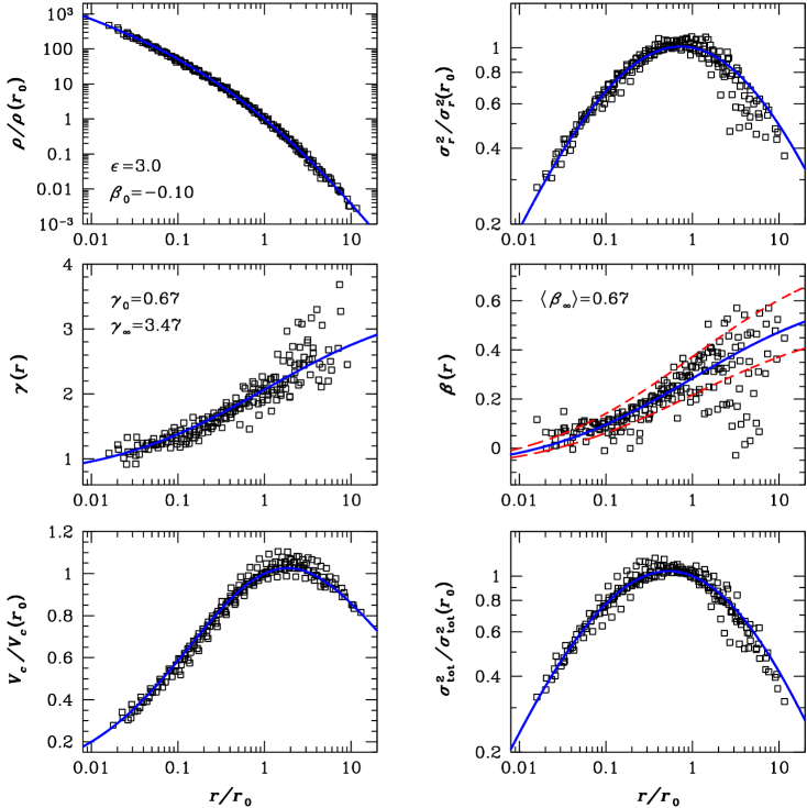
Figure 3: Comparison of our analytical, ’critical-$\alpha$’ models in equation (40) with the same ten simulated CDM haloes from Diemand et al. (2004a, b) that have already been employed in Fig. 1. The exponent $\epsilon$ in the $\rho$-$\sigma$ relation (5) was kept fixed at $\epsilon=3$, while a global $\beta_{0}$ was fit to the density and velocity dispersion profiles of all haloes simultaneously. For each halo, individual values for the scale radius $r_{0}$, normalisation constant $M_{\mathrm{tot}}$, and asymptotic anisotropy $\beta_{\infty}$ at $r\to\infty$ have been fitted (see text for more details). The solid curves show the dimensionless model profiles given the global $\epsilon$ and $\beta_{0}$. Squares represent the data from the simulated haloes, with the various profiles for each halo scaled by their best-fit values at the fitted $r_{0}$ for that particular halo. For the anisotropy profile, the solid curve represents a mean model, in the sense of a mean value for $\beta_{\infty}$, while the dashed curves indicate the range of best-fit values for $\beta_{\infty}$.

Thus, we start by assuming that all haloes follow the same $\rho$-$\sigma$ relation, $\rho/\sigma_{r}^{\epsilon}\propto r^{-\alpha_{\mathrm{crit}}}$, with a single value of $\epsilon$. That this is likely so is already suggested by Figure 1. We further assume that the central velocity anisotropy $\beta_{0}$ is the same for all haloes. This is more of a debatable contention—even though most simulations show similar (low) levels of anisotropy in their innermost resolved regions, there is no clear evidence that $\beta_{0}$ always tends to a single value. Nevertheless, if $\epsilon$ and $\beta_{0}$ both are ‘universal’ then the shape of the density profile must be too in these models, and so this possibility is worth examining.

We proceed by defining a grid of ($\epsilon,\beta_{0}$) values. For each pair in turn, we compute $\eta$, $\gamma_{0}$, and $\gamma_{\infty}$ from equations (36), which allows for the calculation of dimensionless model profiles $\rho_{\mathrm{mod}}(r)$ and $\sigma_{r,\mathrm{mod}}^{2}(r)$. For each of the ten haloes, we then find values for $M_{\mathrm{tot}}^{(j)}$, $r_{0}^{(j)}$, and $\beta_{\infty}^{(j)}$ to minimise the sum of absolute deviations,

$$\Delta_{j}(\epsilon,\beta_{0})=\sum_{i=1}^{N_{j}}\left\{\left|\log\frac{\rho_{\mathrm{mod}}(r_{i})}{\rho(r_{i})}\right|+\epsilon\left|\log\frac{\sigma_{r,\mathrm{mod}}(r_{i})}{\sigma_{r}(r_{i})}\right|\right\},$$ (41)

which is more robust against outliers than the standard $\chi^{2}$ statistic. Here $N_{j}$ is the number of data points in the $j$th halo; typically, $N_{j}=21$. The total deviation that is minimised for each ($\epsilon,\beta_{0}$) is thus

$$\Delta_{\mathrm{tot}}(\epsilon,\beta_{0})=\sum_{j=1}^{N_{\mathrm{halo}}}\Delta_{j}(\epsilon,\beta_{0})\ .$$ (42)

Ultimately, we find the set $\{\epsilon,\beta_{0};M_{\mathrm{tot}}^{(j)},r_{0}^{(j)},\beta_{\infty}^{(j)},j=1,\dots,10\}$ for which $\Delta_{\mathrm{tot}}$ is the minimum over our original grid. Strictly speaking, this occurs at $\epsilon=3.2$ and $\beta_{0}=-0.05$, but the minimum is rather shallow and the best fit with $\epsilon=3$ exactly (which requires $\beta_{0}=-0.10$) is not significantly worse. The details of this latter fit are shown in Figure 3.

The upper panels of Figure 3 show the density and (radial) velocity-dispersion data that were used to constrain the model parameters. To emphasise the shapes of the distributions, the radial coordinate in each halo $j$ has been normalised by the fitted value of $r_{0}^{(j)}$, and the densities and velocity dispersions have been normalised by their fitted values at $r_{0}^{(j)}$. The best-fitting dimensionless profiles, from equations (40b) and (40e), are drawn as the bold curves. The rms relative deviations from these curves, $(\rho-\rho_{\mathrm{mod}})/\rho$ and $(\sigma_{r}^{2}-\sigma_{r,\mathrm{mod}}^{2})/\sigma_{r}^{2}$, are both of order 11%–12% for all ten haloes combined.

The left-middle panel of Figure 3 shows the negative logarithmic density gradient $\gamma(r)$ as a function of $r/r_{0}^{(j)}$ in the simulated haloes against the model curve given by equation (40c) for $\epsilon=3$ and $\beta_{0}=-0.10$. Given these parameters, equations (36) imply that the power-law slopes at $r\to 0$ and $r\to\infty$ are $\gamma_{0}=2/3$ and $\gamma_{\infty}=52/15=3.4\overline{6}$, respectively. The transition from the inner to the outer power law is rather gradual, with $\eta=7/15=0.6\overline{6}$. Recall that $r_{0}$ is defined as the radius at which $\gamma(r_{0})=\gamma_{1}$, with $\gamma_{1}=\tfrac{1}{2}(\gamma_{0}+\gamma_{\infty})=31/15$ in this case.

The right-middle panel then shows the ‘observed’ anisotropy parameter $\beta(r)$ vs. the scaled radius $x=r/r_{0}^{(j)}$. The bold curve traces the model relation (40d) for $\beta_{0}=-0.10$ and $\beta_{\infty}=0.67$, which is the average of the ten different $\beta_{\infty}^{(j)}$ values obtained by fitting the $\sigma_{r}^{2}$ profile of each halo separately. The dashed curves have the same $\beta_{0}=-0.10$ but $\beta_{\infty}=0.53$ and $\beta_{\infty}=0.84$, corresponding to the minimum and maximum of the fits to the ten haloes. Evidently, these curves together account for much of the observed scatter in $\beta(r)$. Note that the average $\beta_{\infty}$ value implies a slope for the $\beta$-$\gamma$ relation (39) of $(\beta_{\infty}-\beta_{0})/(\gamma_{\infty}-\gamma_{0})\simeq 0.28$. This is comparable to the slope $\mathrm{d}\beta/\mathrm{d}\gamma\approx 0.19$ inferred by Hansen & Moore (2005) from their investigations of a completely different set of simulated haloes. However, it should also be noted that Hansen & Moore found a relatively tight correlation between $\beta$ and $\gamma$ (see their Figure 2). Comparison of the data points in the two middle panels of our Figure 3 shows somewhat more scatter in any empirical $\beta$-$\gamma$ relation for the haloes we are working with. This is particularly evident at relatively large radii, $r/r_{0}\ga 2$. In fact, it is not clear that a ‘universal’ slope in a linear $\beta$-$\gamma$ relationship (i.e., a unique value of $\beta_{\infty}$) can describe all of these data if the density profile is strictly ’universal’ (i.e. if there truly is a single value for $\beta_{0}$ as well as $\epsilon$).

The bottom two panels of Figure 3 complete the comparison with our models. The left panel shows the re-normalised circular-velocity profile, $\sqrt{M(r)r_{0}/M(r_{0})r}$ vs. $r/r_{0}$, which is essentially equivalent to the top-left panel showing the model and observed density profiles. The right-hand panel shows the normalised total one-dimensional velocity dispersion profile, which is obtained from the two panels above it: $\sigma_{\mathrm{tot}}^{2}(r)=\sigma_{r}^{2}(r)(1-2\beta(r)/3)$. Note that the scatter of $\sigma_{\mathrm{tot}}^{2}$ about our model is some 25% smaller than that of $\sigma_{r}^{2}$: the scatter away from the model curve in the upper-right panel is compensated by the scatter of $\beta(r)$ in the middle-right panel.

Overall, it is surprising how well our simple model is able to reproduce the main features of the spatial structure and the kinematics of these simulated dark-matter haloes. However, it remains to be checked that the $\rho$-$\sigma$ relation in the ‘observed’ haloes is consistent with that required by the analytical models we have fit. Specifically, by using equations (40) we have assumed that the value of $\alpha$ is the critical one given by equation (31). For $\epsilon=3$ and $\beta_{0}=-0.10$ as in Figure 3, this is $\alpha_{\mathrm{crit}}=59/30=1.9\overline{6}$. Figure 4 plots the $\rho/\sigma_{r}^{3}$ data points from the ten Diemand et al. haloes (normalised by our fitted values of $\rho_{0}^{(j)}$ and $\sigma_{r,0}^{(j)}$ for each halo individually) against the scaled radius $r/r_{0}^{(j)}$. The dashed line has slope $-\alpha_{\mathrm{crit}}$ and gives a reasonable description of the data. In fact, direct linear regression (with a 3-$\sigma$ clipping applied) yields a best-fit slope of $-1.933$, only$\simeq$1.5% different from the expected value. This is drawn as the solid line in Fig. 4. The relative residuals from the critical-$\alpha$ model line, $[(\rho/\sigma_{r}^{3})-(\rho/\sigma_{r}^{3})_{\mathrm{mod}}]/(\rho/\sigma_{r}^{3})$, are shown in the lower panel. Evidently, the largest deviations from this power law occur at $r/r_{0}\ga 2$, which is where the $\sigma_{r}^{2}(r)$ and $\beta(r)$ profiles scatter most in Figure 3.

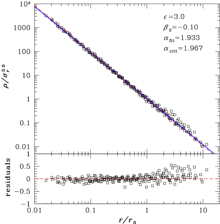
Figure 4: Top panel: plot of $\rho/\sigma_{r}^{3}$ against radius for the ten simulated CDM haloes already employed in Figs. 1 and 3. In fact, this plot is very similar to the right panel of Fig. 1, the only distinction being that we use our best-fit values for individual scale radii $r_{0}^{(j)}$ to normalise the data in each halo. The solid line gives the best-fit power-law relation, with exponent $\alpha_{\mathrm{fit}}=1.933$. The dashed line is the power law implied by the fit of our critical-$\alpha$ model to the haloes’ density and velocity-dispersion profiles in Figure 3: with $\epsilon=3$ and $\beta_{0}=-0.10$, $\alpha_{\mathrm{crit}}=1.9\overline{6}$. Bottom panel: Relative residuals of $(\rho/\sigma_{r}^{3})$ about the latter, critical-$\alpha$ power law assumed by our model fit.

As a last test, we wish to compare our model against the estimated density profile only of an extremely high-resolution halo simulated by Diemand et al. (2005). This is again a cluster-sized halo. As Diemand et al. describe in detail, this particular halo was defined by first performing a simulation with spatial resolution of $10^{-3}$ in units of the virial radius, evolving the run to a high redshift. The most central part of the density profile was then scaled to match onto the outer parts of a lower-resolution halo previously evolved to $z=0$. Because of this estimation procedure, we do not have the full velocity-dispersion and anisotropy profiles for this cluster.

Even in the absence of kinematical data, we can fit for all of $\epsilon$, $\beta_{0}$, $M_{\mathrm{tot}}$, and $r_{0}$ using the density profile alone. In practice, we set $\epsilon=3$ and only fit for $\beta_{0}$ and the two normalisation factors by minimising the sum of absolute deviations $\Delta=\sum_{i}\left|\log\,\rho_{\mathrm{mod}}(r_{i})-\log\,\rho(r_{i})\right|$. In this case, the shape of the density profile at small $r$ requires a slightly larger $\beta_{0}$ than we found for Figure 3: $\beta_{0}\simeq 0.03$ (which, reasonably, is still nearly isotropic). This is one indication that dark-matter halo density profiles may not be exactly universal after all, even if the value of $\epsilon$ is. Some of the scatter found in $\gamma$ at the resolution limit of numerous simulations (e.g., Navarro et al., 2004; Diemand et al., 2004b; Fukushige et al., 2004) may in fact be real and, in our model at least, connected to non-universal halo kinematics.

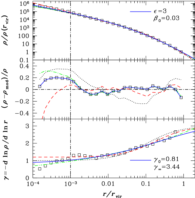
Figure 5: Comparison of the best fit (blue solid curves) of equation (40b) to the high resolution (‘billion particle’) halo of Diemand et al. (2005). For this fit, $\epsilon=3$ was fixed a priori and only $\beta_{0}$, $r_{0}$, and $M_{\mathrm{tot}}$ were allowed to vary. The vertical dot-dashed line indicates the resolution limit of the simulation, according to Diemand et al.. The black dotted, green dash-dot, and red long-dashed curves correspond to the best fits of the profiles proposed by, respectively, Navarro et al. (1996) (see eq. [43]), Navarro et al. (2004) (eq. [44]), and Diemand et al. (2005) (eq. [45]).

The top panel of Figure 5 plots the best fit of equation (40b) against the data for this one halo, now with the virial radius $r_{\mathrm{vir}}$ taken as the normalisation point; this model is given by the solid (blue) curve. For comparison with other fitting functions employed in the literature, we have also found the best-fitting NFW profile,

$$\rho(r)/\rho_{2}=4\,(r/r_{2})^{-1}(1+r/r_{2})^{-2}\ ,$$ (43)

which we show as the dotted (black) curve. The best-fitting function of the type suggested by Navarro et al. (2004),

$$\rho(r)/\rho_{2}=\exp\left\{-\left(2/\alpha_{N}\right)\left[\left(r/r_{2}\right)^{\alpha_{N}}-1\right]\right\},$$ (44)

is shown as the dash-dot (green) curve. Here $\alpha_{N}$ is a free parameter in the fit, which we find to be $\alpha_{N}=0.144$. Finally, the fitting formula preferred by Diemand et al. (2005),

$$\rho(r)/\rho_{s}=2^{1.8}\,(r/r_{s})^{-1.2}(1+r/r_{s})^{-1.8}\ ,$$ (45)

is drawn as the long-dashed (red) curve. Within the resolved radial range of the simulation, $r/r_{\mathrm{vir}}\geq 10^{-3}$, there is little obvious difference between these fits in a plot of $\rho$ vs. $r$.

In the middle panel of Figure 5 we show the fractional residuals from each of the four models fitted to $\rho(r)$. The points joined by the solid blue curve denote the residuals from the fit of our model; residuals from the others just listed are in the same line types and colours as in the upper panel. The NFW model is clearly worse than any of the others, but the remaining three are competitive. The rms fractional density residual about the best NFW fit is 16%; that about the Navarro et al. function is 6.3%; that about the Diemand et al. (2005) formula is 5.2%; and that about our model with $\epsilon=3$ and $\beta_{0}=0.03$ is 6.0%. The main source of the slightly higher global scatter in our model vs. the fitting function of Diemand et al. is the single density point closest to the resolution limit of this simulation.

It is noteworthy that our best-fit dynamical model is almost identical to the best-fitting Navarro et al. function within the resolved radial range, as the latter has been shown to provide a very accurate description of many simulated dark-matter haloes (e.g., Navarro et al., 2004; Diemand et al., 2004b). At some level, it is not surprising that either of these curves is an improvement over, say, the NFW profile, since the former both involve three free parameters in $\rho(r)$ (recall that we fixed $\epsilon=3$ in fitting our model to this halo) while the NFW function contains only two. The advantage to our model, of course, is that the extra degree of freedom in fitting the density profile is also used simultaneously to predict the anisotropic kinematics of the halo. For example, from equation (31) we would predict $\alpha=\alpha_{\mathrm{crit}}=1.938$ in the $\rho$-$\sigma$ relation (5) for this halo. Perhaps coincidentally, this is almost exactly the $\alpha_{\mathrm{fit}}$ found in Figure 4 for the ten lower-resolution haloes from Diemand et al. (2004a, b).

Finally, the bottom panel of Figure 5 shows the negative logarithmic density slope estimated as a function of radius directly from the data of Diemand et al. (2005), against the behaviours predicted by each of the four fits to the density profile. With $\epsilon=3$ and $\beta_{0}=0.03$, our model has $\gamma\to\gamma_{0}=0.81$ as $r\to 0$, and $\gamma\to\gamma_{\infty}=3.44$ as $r\to\infty$. The rollover to $\gamma_{0}$ is very gradual however (from eq. [36a], $\eta=0.438$ here) and at the resolution limit of the simulation we still find $\gamma\simeq 1$ for the fit. Apparently, still higher-resolution simulations are required to distinguish clearly between our density model and others, such as that of Diemand et al., with different asymptotic slopes in the limit $r\to 0$.

5 Summary and discussion

As a rule, investigations into the structure of simulated dark-matter haloes have focused on the nearly ’universal’ shape of their density profiles. This approach is plagued, however, by the fact that the haloes are only ever resolved over 2–3 decades in radius. Since the logarithmic density slope clearly varies smoothly over this entire range, in a way that is not anticipated from any first principles, it is then difficult to characterise unambiguously the true form of $\rho(r)$ with necessarily ad hoc, empirical fitting functions. In particular, the value of the asymptotic central power-law slope (if a single, universal asymptote even exists in the limit $r\to 0$) remains ill-constrained. Thus, the starting point of our analysis in this paper was the remarkable, and much simpler, empirical fact (Taylor & Navarro 2001, see also Hansen 2004) that simulated haloes satisfy, over their whole resolved range, a $\rho$-$\sigma$ relation of the general form

$$\frac{\rho(r)}{\sigma_{r}^{\epsilon}(r)}\propto r^{-\alpha}$$

for $\sigma_{r}$ the radial component of velocity dispersion, and $\epsilon\simeq 3$. (As it happens, using the total one-dimensional velocity dispersion also leads to a nearly power-law $\rho$-$\sigma$ relation, with a slightly different value for $\alpha$; see Taylor & Navarro, and Figure 1 above.) A single power-law dependence such as this is clearly easier to recognise, and to quantify accurately, than is a radius-dependent curvature in the density profile. It is also the simplest nontrivial form that any halo relation could take, and hence the $\rho$-$\sigma$ scaling may be the most fundamental aspect of dark-matter haloes.

We should note here that, while $\rho/\sigma^{3}$ has the dimension of phase-space density, its interpretation as phase-space density (Taylor & Navarro, 2001; Williams et al., 2004), coarse-grained or not, is problematic. On the other hand however, if the phase-space density were in some sense of power-law form, we might expect $\rho/\sigma^{3}$ to closely, but not exactly, follow a power law, too.

Our basic assumption has been that a power-law $\rho$-$\sigma$ relation holds for all radii, not just those resolved by simulations. It is then possible to use this as a constraint on the spherical Jeans equation in order to derive the density profile of an equilibrium halo. In Section 2 we did just this, for a specialised case with $\epsilon=3$ fixed and velocity isotropy assumed. This part of the analysis is thus similar to the original work of Taylor & Navarro (2001), and to aspects of Williams et al. (2004, see also Hansen 2004). However, our study has expanded considerably on these others, as we investigated the full space of all physical solutions to the isotropic Jeans equation under a power-law $\rho$-$\sigma$ relation with arbitrary exponent $\alpha$. Most importantly, we have found that only one solution $\rho(r)$ exists which asymptotes to realistic power-law behaviour in the limits of both small and large radii. This solution occurs only for a single critical value of $\alpha$ and, for this one solution only, the density, velocity-dispersion, and enclosed-mass profiles are all fully analytic.

In Section 3 we extended our analysis by allowing for arbitrary exponents $\epsilon$ in the $\rho$-$\sigma$ relation and, unlike any other detailled study before, for velocity anisotropy. We found that the problem remains analytically tractable for any $\epsilon>2$, only if we adopt a $\rho$-$\sigma$ relation involving the radial component $\sigma_{r}$ of velocity dispersion rather than the total (empirically both are equally well motivated, see Fig. 1) and if we assume the anisotropy parameter $\beta(r)\equiv 1-\sigma_{\theta}^{2}/\sigma_{r}^{2}$ to be either spatially constant or linearly dependent on the logarithmic density slope $\gamma(r)\equiv-\mathrm{d}\ln\,\rho/\mathrm{d}\ln\,r$. Under these reasonable assumptions, there always exists an exact analogue to the fully analytical density profile we found in the isotropic, $\epsilon=3$ case. This solution again occurs for a particular, ‘critical’ $\alpha$ value. Moreover, for the realistic case of $\beta$ linearly increasing with $\gamma$ (corresponding to outwards ever more radially biased anisotropy), this is the only physical solution which resembles simulated dark-matter haloes.

This result is gratifying for two reasons. First, it connects neatly with an entirely independent, empirical finding by Hansen & Moore (2005), who have argued on the basis of a variety of simulations that indeed there exists a roughly linear relation between $\beta(r)$ and $\gamma(r)$ in collisionless haloes formed through numerous different processes. Second, it turns out that the slope of this linear ‘$\beta$-$\gamma$ relation’ does not affect the critical value of $\alpha$, nor does it affect the shape of the equilibrium $\rho(r)$ profile itself. Rather, both of these things are influenced only by the central anisotropy $\beta_{0}\equiv\beta(r=0)$. Specifically, for a $\rho$-$\sigma$ relation with $\epsilon=3$ (which ultimately does appear to be most appropriate), our solution of the Jeans equation with radially varying velocity anisotropy requires

$$\frac{\rho}{\sigma_{r}^{3}}\propto r^{-\frac{35}{18}+\frac{2}{9}\beta_{0}}$$ (46a)

and has density

$$\rho(r)\propto x^{-\frac{7+10\beta_{0}}{9}}\left(1+x^{\frac{2(2-\beta_{0})}{9}}\right)^{-6},$$ (46b)

with $$x\equiv r/r_{0}$$, radial velocity dispersion

$$\sigma_{r}^{2}(r)\propto x^{\frac{7-8\beta_{0}}{9}}\left(1+x^{\frac{2(2-\beta_{0})}{9}}\right)^{-4},$$ (46c)

and anisotropy

$$\beta(r)\equiv 1-\frac{\sigma_{\theta}^{2}(r)}{\sigma_{r}^{2}(r)}=\frac{\beta_{0}+\beta_{\infty}x^{2(2-\beta_{0})/9}}{1+x^{2(2-\beta_{0})/9}}$$ (46d)

for any $\beta_{0}\leq 1$, $\beta_{\infty}\leq 1$. Thus, the halo density profile has a shallow power-law cusp, $\rho\to r^{-(7+10\beta_{0})/9}$ in the limit $r\to 0$, and steepens monotonically but slowly to $\rho\to r^{-(31-2\beta_{0})/9}$ as $r\to\infty$. More general results for $\epsilon\neq 3$ in the $\rho$-$\sigma$ relation, including analytical expressions for the velocity-dispersion, enclosed-mass, and circular-velocity profiles, are given in equations (40) above (with auxiliary definitions in eqs. [36]).

In Section 4 we fit our analytical, critical-$\alpha$ density and velocity-dispersion profiles to those in ten dark-matter haloes simulated by Diemand et al. (2004a, b). When modelling these ’data’, we assumed that all haloes obey a $\rho$-$\sigma$ relation with a single value of $\epsilon$ and have the same central velocity anisotropy $\beta_{0}$, so that the halo density profile is necessarily universal. We were able to find a good fit to all ten haloes simultaneously for $\epsilon=3$ and $\beta_{0}=-0.10$, only slightly different from isotropic; see Figure 3. For this combination of parameters, our model requires $\rho/\sigma_{r}^{3}\propto r^{-1.9\overline{6}}$ for self-consistency, and we showed in Figure 4 that this is a satisfactory description of the data.

In Section 4 we also fit our model to the density profile of an extremely high-resolution (’billion-particle’) halo simulated by Diemand et al. (2005), finding good agreement again with $\epsilon=3$ and a nearly isotropic $\beta_{0}=0.03$. In this case the fitted density profile has a central power-law cusp $\rho\to r^{-0.81}$ as $r\to 0$, which steepens gradually to $\rho\to r^{-3.44}$ as $r\to\infty$; see Figure 5. At the resolution limit of the Diemand et al. simulation (about 0.001 of the virial radius), the fit has $\gamma\simeq 1$, significantly larger than the asymptotic cusp slope and still consistent with both the simulation data and the behaviour of other fitting functions. Within the resolved radial range, our model fit is also very closely traced by the best fit of the ad hoc profile proposed by Navarro et al. (2004).

Our findings suggest a possible first-principles explanation for halo density profiles along the following line of arguments. The initial distribution function before collapse was completely cold (a $\delta$-function in velocity space) and hence the phase-space density scale-free. The collapse and the subsequent process of violent relaxation (phase-space mixing) is driven by gravity alone, which cannot introduce any scale dependence. This implies that the phase-space density of the collapsed halo satisfies some form of scale invariance, suggesting that the ratio $\rho(r)/\sigma^{3}$, which is closely related to the phase-space density, follows a power law (the general scale-invariant functional form). However, as our analysis has shown, if $\rho(r)/\sigma^{3}$ of dark-matter haloes is any power of radius, then the condition of equilibrium (and physically sensible density profiles) requires the particular power law $r^{-\alpha_{\mathrm{crit}}}$ and, simultaneously, that the density profile follows that given above.

From our fits to simulated haloes in Section 4, the $\beta$-$\gamma$ relation seems not as tight or universal as the $\rho$-$\sigma$ relation. This is not very surprising, since different amounts of velocity anisotropy are required to stabilise different spatial halo shapes, resulting in some scatter between the $\beta$-$\gamma$ relations of different haloes. Since only the central velocity anisotropy $\beta_{0}$ affects the value of $\alpha_{\mathrm{crit}}$, this scatter has little (or no) influence on the the $\rho$-$\sigma$ relation as long as $\beta_{0}$ is similar (or the same) for different haloes. This explains why haloes of different spatial shape still have very similar density profiles. Whether $\beta_{0}$ is a universal parameter (close to zero) or whether there is some real scatter we cannot predict, but in Section 4 we obtained a good fit to ten different simulated haloes using a single value for $\beta_{0}$ (see Fig. 3).

Of course, our analysis is still restricted to spherical symmetry and ignores any halo substructure. However, substructure is unimportant for the issue of the overall density profile, as simulations of dark-matter structure formation with suppressed small-scale power in the initial conditions still yield the same characteristic density profiles, but much less substructure (Moore et al., 1999). The issue of asphericity is more likely to be relevant and hence it is all the more remarkable that our spherical analysis gives such a good description of the spherically averaged profiles. Evidently, anisotropy, which was ignored in previous studies, is presumably more important than asphericity, because the gravitational potential is always less aspherical than the density distribution.

References

- Ascasibar et al. (2004) Ascasibar Y., Yepes G., Gottlöber S., Müller V., 2004, MNRAS, 352, 1109
- Bertschinger (1985) Bertschinger E., 1985, ApJS, 58, 39
- Bullock et al. (2001) Bullock J. S., Kolatt T. S., Sigad Y., Somerville R. S., Kravtsov A. V., Klypin A. A., Primack J. R., Dekel A., 2001, MNRAS, 321, 559
- Carlberg et al. (1997) Carlberg R. G., Yee H. K. C., Ellingson E., Morris S. L., Abraham R., Gravel P., Pritchet C. J., Smecker-Hane T., Hartwick F. D. A., Hesser J. E., Hutchings J. B., Oke J. B., 1997, ApJ, 485, L13
- Cole & Lacey (1996) Cole S., Lacey C., 1996, MNRAS, 281, 716
- Colín et al. (2000) Colín P., Klypin A. A., Kravtsov A. V., 2000, ApJ, 539, 561
- Crone et al. (1994) Crone M. M., Evrard A. E., Richstone D. O., 1994, ApJ, 434, 402
- Diemand et al. (2004a) Diemand J., Moore B., Stadel J., 2004a, MNRAS, 352, 535
- Diemand et al. (2004b) Diemand J., Moore B., Stadel J., 2004b, MNRAS, 353, 624
- Diemand et al. (2005) Diemand J., Zemp M., Moore B., Stadel J., Carollo M., 2005, MNRAS, submitted (astro-ph/0504215)
- Dubinski & Carlberg (1991) Dubinski J., Carlberg R. G., 1991, ApJ, 378, 496
- Fukushige et al. (2004) Fukushige T., Kawai A., Makino J., 2004, ApJ, 606, 625
- Fukushige & Makino (1997) Fukushige T., Makino J., 1997, ApJ, 477, L9
- Fukushige & Makino (2001) Fukushige T., Makino J., 2001, ApJ, 557, 533
- Ghigna et al. (1998) Ghigna S., Moore B., Governato F., Lake G., Quinn T., Stadel J., 1998, MNRAS, 300, 146
- Ghigna et al. (2000) Ghigna S., Moore B., Governato F., Lake G., Quinn T., Stadel J., 2000, ApJ, 544, 616
- Hansen & Moore (2005) Hansen S., Moore B., 2005, MNRAS, submitted (astro-ph/0411473)
- Hansen (2004) Hansen S. H., 2004, MNRAS, 352, L41
- Hayashi et al. (2004) Hayashi E., Navarro J. F., Power C., Jenkins A., Frenk C. S., White S. D. M., Springel V., Stadel J., Quinn T. R., 2004, MNRAS, 355, 794
- Hernquist (1990) Hernquist L., 1990, ApJ, 356, 359
- Merritt et al. (2005) Merritt D., Navarro J. F., Ludlow A., Jenkins A., 2005, ApJ, 624, L85
- Moore et al. (1998) Moore B., Governato F., Quinn T., Stadel J., Lake G., 1998, ApJ, 499, L5
- Moore et al. (1999) Moore B., Quinn T., Governato F., Stadel J., Lake G., 1999, MNRAS, 310, 1147
- Navarro et al. (1996) Navarro J. F., Frenk C. S., White S. D. M., 1996, ApJ, 462, 563
- Navarro et al. (1997) Navarro J. F., Frenk C. S., White S. D. M., 1997, ApJ, 490, 493
- Navarro et al. (2004) Navarro J. F., Hayashi E., Power C., Jenkins A. R., Frenk C. S., White S. D. M., Springel V., Stadel J., Quinn T. R., 2004, MNRAS, 349, 1039
- Plummer (1911) Plummer H. C., 1911, MNRAS, 71, 460
- Power et al. (2003) Power C., Navarro J. F., Jenkins A., Frenk C. S., White S. D. M., Springel V., Stadel J., Quinn T., 2003, MNRAS, 338, 14
- Press et al. (1992) Press W. H., Teukolsky S. A., Vetterling W. T., Flannery B. P., 1992, Numerical Recipies in C, 2nd edn. Cambridge, Cambridge University Press
- Rasia et al. (2004) Rasia E., Tormen G., Moscardini L., 2004, MNRAS, 351, 237
- Stoehr et al. (2002) Stoehr F., White S. D. M., Tormen G., Springel V., 2002, MNRAS, 335, L84
- Taylor & Navarro (2001) Taylor J. E., Navarro J. F., 2001, ApJ, 563, 483
- Williams et al. (2004) Williams L. L. R., Austin C., Barnes E., Babul A., Dalcanton J., 2004, in Dettmar R., Klein U., Salucci P., eds, Baryons in Dark Matter Halos Proceedings of Science. pp 20–23
- Zhao (1996) Zhao H., 1996, MNRAS, 278, 488